Embed Size (px)
Citation preview

A quantitative study of the lift-enhancing flow field generated by an airfoil with a Gurney flap
A DISSERTATION SUBMITTED TO THE FACULTY OF THE GRADUATE SCHOOL
OF THE UNIVERSITY OF MINNESOTA BY
Daniel Ryan Troolin
IN PARTIAL FULFILLMENT OF THE REQUIREMENTS FOR THE DEGREE OF
DOCTOR OF PHILOSOPHY
Ellen K. Longmire, Adviser
December 2009

© Daniel Ryan Troolin 2009

i
Acknowledgements I would like to thank my adviser Prof. Ellen Longmire for her wisdom, guidance, and support. I consider myself very fortunate to be counted as one of her students. I would also like to thank: The rest of my examining committee Prof. Ivan Marusic, Prof. Krishnan Mahesh, and Prof. Terry Simon for sharing their expertise with me. The department of Aerospace Engineering and Mechanics and TSI Incorporated for the financial support. My wife Danica and my kids Madeline and John Robert (who was born during a finals week) for their moral and emotional support, and our parents for their help and guidance. Dr. Wing Lai for encouraging me when things seemed impossible. And finally, God for the miracle that has been my graduate school experience.

ii
Dedication This dissertation is dedicated to my wonderful parents, whom I love deeply.

iii
Abstract
Although it is well known that a Gurney flap affects the lift, drag, and pressure
distribution along an airfoil, the mechanisms behind the changes are still not well
understood. The following research seeks to understand what is causing the effects of a
Gurney flap through quantitative measurements of the spatial and temporal flow details,
including force balance measurements, hotwire anemometry (HWA), high resolution
particle image velocimetry (HRPIV), and time resolved particle image velocimetry
(TRPIV). TRPIV is used to broaden the understanding of the interaction between the
various vortex shedding modes which are elicited from the regions upstream and
downstream of the flap. The HWA technique is useful for its very high frequency
response, and is used in the wake of the airfoil in order to gain valuable insight into the
nature of the vortex shedding frequencies. Vortices generated both upstream and
downstream of the Gurney flap have been observed, and the vortex interactions, which
occur due to the non-phase-locked nature of the shedding modes, are analyzed. The
results are interpreted in terms of the known lift increment.

iv
Table of Contents List of Tables.................................................................................................................. vii
List of Figures................................................................................................................ viii
Nomenclature ................................................................................................................ xiv
1 Introduction ............................................................................................................... 1
1.1 Motivation........................................................................................................ 1
1.2 Previous Work ................................................................................................. 3
1.2.1 Low Reynolds Number Airfoil Characteristics...................................... 3
1.2.2 Previous Work on Gurney Flaps ............................................................ 6
1.2.2.1 Lift and Drag Characteristics........................................................ 6
1.2.2.2 Delayed Separation..................................................................... 11
1.2.2.3 Boundary Layer Effects.............................................................. 13
1.2.2.4 Flow Control............................................................................... 14
1.2.2.5 Perturbed Gurney Flaps.............................................................. 17
1.2.2.6 Specific Applications.................................................................. 18
1.3 Objectives and Approach............................................................................... 20
2 Experimental Apparatus and Methods .................................................................... 23
2.1 Wind Tunnel Facility..................................................................................... 23
2.2 Airfoil Characteristics.................................................................................... 25
2.3 Freestream Velocity Characteristics .............................................................. 32
2.3.1 Blockage Effects .................................................................................. 32
2.4 Force Balance ................................................................................................ 34
2.4.1 Correction to Infinite Aspect Ratio and Wall Influence ...................... 34
2.5 Hotfilm Anemometry..................................................................................... 36
2.5.1 Principle of Hotfilm Anemometry ....................................................... 36
2.5.2 Converting Voltage to Effective Velocity............................................ 37
2.5.3 Anemometer Frequency Response....................................................... 39
2.5.4 Hot Film Probes ................................................................................... 39

v
2.5.5 Hot film Calibration ............................................................................. 41
2.5.6 Free Stream Velocity Measurements ................................................... 43
2.5.7 Shedding Frequency Measurements .................................................... 43
2.6 Particle Image Velocimetry (PIV) ................................................................. 44
2.6.1 Seeding................................................................................................. 46
2.6.2 Illumination.......................................................................................... 49
2.6.3 Image Capture ...................................................................................... 52
2.6.4 Timing Synchronization....................................................................... 56
2.6.5 Calibration............................................................................................ 59
2.6.6 PIV Processing ..................................................................................... 60
2.6.6.1 Image Pre-Processing ................................................................. 60
2.6.6.2 Interrogation and Cross Correlation ........................................... 61
2.6.6.3 CDIC Deformation Method........................................................ 63
2.6.6.4 Time Resolved PIV .................................................................... 64
2.6.6.5 High Resolution PIV .................................................................. 64
2.6.6.6 Vector Validation ....................................................................... 64
2.7 Uncertainty .................................................................................................... 65
2.7.1 Lift Coefficient Uncertainty................................................................. 65
2.7.2 Hot film Anemometry Uncertainty ...................................................... 67
2.7.3 Particle Image Velocimetry Uncertainty.............................................. 68
3 Results and Discussion: Force Balance and Flow Visualization ............................ 71
3.1 Force Balance Measurements ........................................................................ 71
3.1.1 Effect of Gurney Flaps on Lift ............................................................. 71
3.1.2 Effect of Filled In Gurney Flap on Lift ................................................ 72
3.2 Tuft Flow Visualization................................................................................. 73
3.2.1 Suction Surface Visualization.............................................................. 73
3.2.2 Pressure Surface Visualization............................................................. 80
4 Results and Discussion: Velocity Measurements................................................... 81
4.1 Time-Averaged Trailing Edge....................................................................... 81

vi
4.2 Time-Averaged Leading Edge....................................................................... 92
5 Results and Discussion: Time Resolved PIV Results ............................................ 98
5.1 Instantaneous PIV Measurements – No Gurney Flap.................................... 98
5.2 Instantaneous PIV Measurements – 4% Gurney Flap ................................. 108
5.3 Instantaneous PIV Measurements – 4% Gurney Flap Filled In .................. 127
6 Results and Discussion: Frequency Measurements ............................................. 132
6.1 Frequency Data – No Gurney Flap.............................................................. 132
6.2 Frequency Data – 4% Gurney Flap ............................................................. 134
6.3 Frequency Data – 4% Gurney Flap Filled In............................................... 138
6.4 Summary 141
7 Conclusions ........................................................................................................... 146
7.1 Force Measurements and Flow Visualization.............................................. 146
7.2 Time-Averaged ............................................................................................ 147
7.3 Time-Resolved............................................................................................. 149
7.4 Frequency .................................................................................................... 150
7.5 Summary and Recommendations for Future Work ..................................... 152
Bibliography ................................................................................................................. 155
A Airfoil Coordinates................................................................................................ 162
B Additional Average PIV Plots............................................................................... 167
C Frequency Data for 2% Gurney Flap .................................................................... 176

vii
List of Tables
Table 2.1: Actual Gurney flap heights.....................................................................28
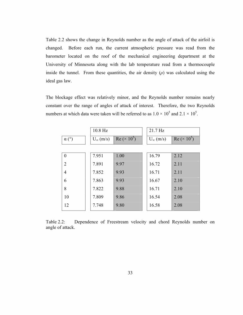
Table 2.2: Dependence of Freestream velocity and chord Reynolds number on angle of attack.........................................................................................33
Table 2.3: Operating resistance, overheat ratio, offset, gain, and operating temperature for the hotfilm probes. ........................................................43
Table 2.4: Significant parameters used in each of the PIV experiments. ................58
Table 6.1: Summary of the primary and secondary shedding frequency for the 2% and 4% Gurney flaps at Re = 2.1 × 10⁵..........................................141
Table 6.2: Summary of the primary and secondary shedding frequency for the 2% and 4% Gurney flaps at Re = 1.0 × 10⁵..........................................142
Table A.1: Coordinates for the standard NACA0015 airfoil..................................163
Table A.2: Coordinates for the NACA0015 airfoil with 1% Gurney flap. ............164
Table A.3: Coordinates for the NACA0015 airfoil with 2% Gurney flap. ............165
Table A.4: Coordinates for the NACA0015 airfoil with 4% Gurney flap. ............166

viii
List of Figures Figure 1.1: Features of a laminar separation bubble. Figure reproduced from
Horton (1968). ..........................................................................................5 Figure 1.2: Gurney flap tested by Liebeck, with the proposed trailing edge
vortex structure. Flow is from left to right. Figure reproduced from Liebeck (1978).................................................................................7
Figure 1.3: Numerically computed particle traces in the vicinity of the NACA 4412 airfoil with a 1.25% Gurney flap at Re = 1.64 × 10⁶. Flow is from left to right. Figure reproduced from Jang et al. (1998). ................8
Figure 1.4: CL vs angle of attach and CD vs CL for an Eppler e423 section at Re = 0.75 - 0.89 × 10⁶ as determined by Jeffrey et al. (2000). Figure reproduced from Jeffrey et al. (2000). ..........................................9
Figure 1.5: The time-averaged LDA streamline results of Jeffrey et al. (4% Gurney, α = 0°). Figure reproduced from Jeffrey et al. (2000). ..............9
Figure 1.6: Instantaneous vorticity contours downstream of an airfoil with a Gurney flap. Figure reproduced from Liebeck (1978). Figure reproduced from Zerihan and Zhang (2001). .........................................10
Figure 1.7: Gurney flap wake structure seen by Neuhart and Pendergraft. Flow is from top to bottom. Figure reproduced from Neuhart and Pendergraft (1988)..................................................................................12
Figure 1.8: Time history of Cl for an impulsively started NACA0012 airfoil with a 1.5% flap attached. Figure reproduced from Lee and Kroo (2004). ....................................................................................................15
Figure 2.1: Drawing of the Wind Tunnel (Courtesy ELD Inc. Reprinted with permission). ............................................................................................24
Figure 2.2: Photo of the wind tunnel.........................................................................25 Figure 2.3: Schematic showing the flow coordinate system.....................................26 Figure 2.4: Schematic drawing of the airfoil with Gurney flap (not to scale). .........27 Figure 2.5: Photo of the airfoil test sections. ............................................................27 Figure 2.6: Photo of the 4% flap configuration attached to the aluminum
mounting plate. .......................................................................................28 Figure 2.7: Photo of the airfoil with 4% Gurney flap mounted in the wind
tunnel. .....................................................................................................29 Figure 2.8: Airfoil section mounted in wind tunnel showing the mounting
bracket. ...................................................................................................30 Figure 2.9: Schematic of the filled-in flap configuration (not to scale)....................31 Figure 2.10: Photo of the filled-in flap configuration. ................................................31 Figure 2.11: Dependence of freestream velocity on angle of attack...........................32 Figure 2.12: A simple CTA circuit. (Courtesy TSI Incorporated)..............................36 Figure 2.13: Schematic of the IFA300 (Courtesy TSI Incorporated). ........................37 Figure 2.14: Model 1210-20 Hotfilm probe schematic. (Courtesy TSI
Incorporated)..........................................................................................40 Figure 2.15: Photo of the model 1210-20 Hotfilm probe. ..........................................40

ix
Figure 2.16: Schematic of the model 1128B hotwire calibrator. (Courtesy TSI Incorporated)..........................................................................................41
Figure 2.17: Hotfilm probe calibrations......................................................................42 Figure 2.18: Schematic of a basic PIV arrangement...................................................45 Figure 2.19: Measured particle size distribution of olive oil seeding particles
generated by a Laskin nozzle particle generator. Reproduced from Thomas and Butefisch (1993). ...............................................................47
Figure 2.20: Photo (left) and schematic (right) showing the internal components including the impactor plate and the Laskin nozzles of the TSI Model 9307 Oil Droplet Generator (Courtesy TSI Incorporated)..........48
Figure 2.21: Laser used for high resolution PIV mounted to the top of the wind tunnel with light sheet optics and mirror. ...............................................49
Figure 2.22: Photo of the TRPIV experimental arrangement. ....................................50 Figure 2.23: Schematic of the PIV arrangement, including the locations of the
laser, laser sheet path, and camera in relation to the PIV area of interest. ...................................................................................................51
Figure 2.24: Schematic representation of the laser light sheet optics. ........................52 Figure 2.25: TSI PowerView 11MP Camera used for high resolution PIV
measurements (Courtesy TSI Incorporated). .........................................53 Figure 2.26: PIV setup with orange-fluorescent rhodamine paint visible on the
airfoil surface..........................................................................................54 Figure 2.27: Rhodamine Paint on an airfoil with laser on. Paint has been
applied on the left side, but not on the right side....................................55 Figure 2.28: Photron APX camera used for time-resolved PIV measurements..........56 Figure 2.29: TSI 610035 LaserPulse Synchronizer (Courtesy TSI Incorporated). ....57 Figure 2.30: Timing diagram for TRPIV image acquisition at 4000 Hz (Δt = 20
μs). ..........................................................................................................57 Figure 2.31: Timing diagram for HRPIV image acquisition (Δt = 5 μs). ...................58 Figure 2.32: PIV calibration target alignment. ...........................................................59 Figure 2.33: Sample calibration image. Dot spacing is 2.5mm. ................................60 Figure 2.34: Background subtraction image preprocessing. Raw image is
shown in the upper left corner, the minimum average intensity image is shown in the upper right corner, and the final image for processing is shown on the bottom.........................................................61
Figure 2.35: Example interrogation pair, image A (left) and image B (right). ...........62 Figure 2.36: Correlation map achieved from images shown in Fig. 2.35...................63 Figure 2.37: Comparison of data from the current study with those acquired in
the NACA facility (Jacobs and Sherman (1937)). All data are corrected to infinite span and free air. ....................................................66
Figure 3.1: CL vs. α for airfoils with Gurney flaps of height 0% (blue), 1% (red), 2% (green), and 4% (orange) at Re = 2.1 × 10⁵............................72
Figure 3.2: CL vs. α for airfoils with 4% Gurney flaps with an open upstream cavity (orange) and closed upstream cavity (blue). The airfoil with 2% flap is shown in red for comparison. Re = 2.1 × 10⁵.......................73
x
Figure 3.3: Tuft flow visualization of the suction surface of the control NACA 0015 airfoil with Reynolds number 1.0 × 10⁵, at (top to bottom) α = 0°, 10°, 12°, and 14°. Flow moves bottom to top. .............................75
Figure 3.4: Tuft flow visualization of the suction surface of the airfoil with 4% Gurney flap with Reynolds number 1.0 × 10⁵, at (top to bottom) α = 0°, 10°, 12°, and 14°. Flow moves bottom to top. .............................76
Figure 3.5: Tuft flow visualization of the suction surface of the control NACA 0015 airfoil with Reynolds number 2.1 × 10⁵, at (top to bottom) α = 0°, 10°, 13°, 15°, and 17°. Flow moves bottom to top.......................78
Figure 3.6: Tuft flow visualization of the suction surface of the airfoil with 4% Gurney flap with Reynolds number 2.1 × 10⁵, at (top to bottom) α = 0°, 10°, 13°, 15°, and 17°. Flow moves bottom to top.......................79
Figure 3.7: Comparison of separation regions on pressure surface of the airfoil with a 4% Gurney flap at α = 0° (left) and 8° (right) at Rec = 1.0 × 10⁵. Flow moves bottom to top..............................................................80
Figure 4.1: Average streamwise velocity on the 0% Gurney flap at Re = 1.0 × 10⁵ for α = 0° (top) and α = 8° (bottom).................................................83
Figure 4.2: Average streamwise velocity on the 0% Gurney flap at Re = 2.1 × 10⁵ for α = 0° (top) and α = 8° (bottom).................................................84
Figure 4.3: Average streamwise velocity on the 4% Gurney flap at Re = 1.0 × 10⁵ for α = 0° (top) and α = 8° (bottom).................................................86
Figure 4.4: Average streamwise velocity on the 4% Gurney flap at Re = 2.1 × 10⁵ for α = 0° (top) and α = 8° (bottom).................................................87
Figure 4.5: Average streamwise velocity (captured using TRPIV) on the 4% Gurney flap at Re = 2.1 × 10⁵ for α = 0° (top) and α = 8° (bottom).......90
Figure 4.6: Average streamwise velocity (captured using TRPIV) on the 4% Gurney flap with the upstream cavity filled in at Re = 2.1 × 10⁵ for α = 0° (top) and α = 8° (bottom).............................................................91
Figure 4.7: Average of 50 PIV fields at the airfoil leading edge at Rec = 1.0 × 10⁵ for the 0% Gurney flap at α = 0° (top) and α = 8° (bottom). Color contours represent normalized streamwise velocity.....................94
Figure 4.8: Average of 50 PIV fields at the airfoil leading edge at Rec = 2.1 × 10⁵ for the 0% Gurney flap at α = 0° (top) and α = 8° (bottom). Color contours represent normalized streamwise velocity.....................95
Figure 4.9: Average of 50 PIV fields at the airfoil leading edge at Rec = 1.0 × 10⁵ for the 4% Gurney flap at α = 0° (top) and α = 8° (bottom). Color contours represent normalized streamwise velocity.....................96
Figure 4.10: Average of 50 PIV fields at the airfoil leading edge at Rec = 2.1 × 10⁵ for the 4% Gurney flap at α = 0° (top) and α = 8° (bottom). Color contours represent normalized streamwise velocity.....................97
Figure 5.1: Normal velocity (v/U∞) downstream of the airfoil without a Gurney flap at Re = 2.1 × 10⁵ and α = 0° (left) and α = 8° (right). ......101
Figure 5.2: Vorticity (ωc/U∞) downstream of the airfoil without a Gurney flap at Re = 2.1 × 10⁵ and α = 0° (left) and α = 8° (right). ..........................102
xi
Figure 5.3: Swirl (λ2Dc/U∞) downstream of the airfoil without a Gurney flap at Re = 2.1 × 10⁵ and α = 0° (left) and α = 8° (right). ..............................103
Figure 5.4: Instantaneous plots of swirl (λ2Dc/U∞) downstream of the airfoil without a Gurney flap at α = 0° and Re = 2.1 × 10⁵. ............................104
Figure 5.5: Instantaneous plots of swirl (λ2Dc/U∞) downstream of the airfoil without a Gurney flap at α = 8° and Re = 2.1 × 10⁵. ............................105
Figure 5.6: Instantaneous plots of swirl (λ2Dc/U∞) downstream of the airfoil without a Gurney flap at α = 0° and Re = 1.0 × 10⁵. ............................106
Figure 5.7: Instantaneous plots of swirl (λ2Dc/U∞) downstream of the airfoil without a Gurney flap at α = 8° and Re = 1.0 × 10⁵. ............................107
Figure 5.8: Normal velocity (v/U∞) downstream of the airfoil with a 4% Gurney flap at α = 0° and Re = 2.1 × 10⁵. ............................................109
Figure 5.9: Vorticity (ωc/U∞) downstream of the airfoil with a 4% Gurney flap at α = 0° and Re = 2.1 × 10⁵. ................................................................110
Figure 5.10: Swirl (λ2Dc/U∞) downstream of the airfoil with a 4% Gurney flap at α = 0° and Re = 2.1 × 10⁵. ....................................................................111
Figure 5.11: Instantaneous plots of swirl (λ2Dc/U∞) downstream of the airfoil without a Gurney flap at α = 0° and Re = 2.1 × 10⁵. ............................113
Figure 5.12: Instantaneous plots of swirl (λ2Dc/U∞) downstream of the airfoil without a Gurney flap at α = 0° and Re = 1.0 × 10⁵. ............................114
Figure 5.13: Normal velocity (v/U∞) downstream of the airfoil with a 4% Gurney flap at α = 8° and Re = 2.1 × 10⁵. Sequence on the left shows constructive upstream shedding. Sequence on the right shows destructive upstream shedding. .................................................118
Figure 5.14: Vorticity (ωc/U∞) downstream of the airfoil with a 4% Gurney flap at α = 8° and Re = 2.1 × 10⁵. Sequence on the left shows constructive upstream shedding. Sequence on the right shows destructive upstream shedding. ............................................................119
Figure 5.15: Swirl (λ2Dc/U∞) downstream of the airfoil with a 4% Gurney flap at α = 8° and Re = 2.1 × 10⁵. Sequence on the left shows constructive upstream shedding. Sequence on the right shows destructive upstream shedding. ............................................................120
Figure 5.16: Instantaneous plots of swirl (λ2Dc/U∞) downstream of the airfoil with a 4% Gurney flap at α = 8° and Re = 2.1 × 10⁵............................122
Figure 5.17: Instantaneous plots of swirl (λ2Dc/U∞) downstream of the airfoil with a 4% Gurney flap at α = 8° and Re = 1.0 × 10⁵............................124
Figure 5.18: Schematic of the bimodal vortex shedding occurring at the trailing edge of the airfoil with a Gurney flap. Positive vorticity is indicated in red; negative vorticity is indicated in blue. The green areas represent fluid “trapped” in the upstream cavity. Arrows represent general trajectories of flow structures. Figure reproduced from Troolin et al. (2006).....................................................................126
Figure 5.19: Normalized normal velocity PDF at the point below the 4% Gurney flap tip at α = 0° and Re = 2.1 × 10⁵. Figure reproduced from Troolin et al. (2006).....................................................................126

xii
Figure 5.20: Normal velocity (v/U∞) downstream of the airfoil with a 4% filled-in Gurney flap at Re = 2.1 × 10⁵ and α = 0° (left) and α = 8° (right). ...................................................................................................129
Figure 5.21: Vorticity (ωc/U∞) downstream of the airfoil with a 4% filled-in Gurney flap at Re = 2.1 × 10⁵ and α = 0° (left) and α = 8° (right). ......130
Figure 5.22: Swirl (λ2Dc/U∞) downstream of the airfoil with a 4% filled-in Gurney flap at Re = 2.1 × 10⁵ and α = 0° (left) and α = 8° (right). ......131
Figure 6.1: Frequency spectra for α = 0°, 4°, 8°, and 12° for the airfoil without a Gurney flap at Re = 2.1 × 10⁵. ...........................................................133
Figure 6.2: Frequency spectra for α = 0°, 4°, 8°, and 12° for the airfoil without a Gurney flap at Re = 1.0 × 10⁵. ...........................................................134
Figure 6.3: Frequency spectra for α = 0°, 4°, 8°, and 12° for the airfoil with a 4% Gurney flap at Re = 2.1 × 10⁵. .......................................................135
Figure 6.4: Peak Strouhal numbers (St = fh/U∞) observed from hot-film spectra at various locations on an airfoil with a 4% Gurney flap at α = 8° and Re = 2.1 × 10⁵. ....................................................................137
Figure 6.5: Frequency spectra for α = 0°, 4°, 8°, and 12° for the airfoil with a 4% Gurney flap at Re = 1.0 × 10⁵. .......................................................138
Figure 6.6: Frequency spectra for α = 0°, 4°, 8°, and 12° for the airfoil with a filled-in 4% Gurney flap at Re = 2.1 × 10⁵..........................................139
Figure 6.7: Frequency spectra for α = 0°, 4°, 8°, and 12° for the airfoil with a filled-in 4% Gurney flap at Re = 1.0 × 10⁵..........................................140
Figure 6.8: Plot of Strouhal number vs. angle of attack for the 2%, 4%, open, and filled flap configurations at Re = 2.1 × 10⁵. ..................................143
Figure 6.9: Instantaneous plots of vorticity (ωc/U∞) downstream of an airfoil with a 4% Gurney flap at α = 0° (top left) and α = 8° (top right), and with a 4% filled Gurney flap at α = 0° (bottom left) and α = 8° (bottom right) at Re = 2.1 × 10⁵. ..........................................................145
Figure B.1: Average Streamwise Velocity on the 1% Gurney flap at Re = 1.0 × 10⁵ for α = 0° (top) and α = 8° (bottom)...............................................168
Figure B.2: Average Streamwise Velocity on the 1% Gurney flap at Re = 2.1 × 10⁵ for α = 0° (top) and α = 8° (bottom)...............................................169
Figure B.3: Average Streamwise Velocity on the 2% Gurney flap at Re = 1.0 × 10⁵ for α = 0° (top) and α = 8° (bottom)...............................................170
Figure B.4: Average Streamwise Velocity on the 2% Gurney flap at Re = 2.1 × 10⁵ for α = 0° (top) and α = 8° (bottom)...............................................171
Figure B.5: Average of 50 PIV fields at the airfoil leading edge at Rec = 1.0 × 10⁵ for the 1% Gurney flap at α = 0° (top) and α = 8° (bottom). Color contours represent normalized streamwise velocity...................172
Figure B.6: Average of 50 PIV fields at the airfoil leading edge at Rec = 2.1 × 10⁵ for the 1% Gurney flap at α = 0° (top) and α = 8° (bottom). Color contours represent normalized streamwise velocity...................173
Figure B.7: Average of 50 PIV fields at the airfoil leading edge at Rec = 1.0 × 10⁵ for the 2% Gurney flap at α = 0° (top) and α = 8° (bottom). Color contours represent normalized streamwise velocity...................174

xiii
Figure B.8: Average of 50 PIV fields at the airfoil leading edge at Rec = 2.1 × 10⁵ for the 2% Gurney flap at α = 0° (top) and α = 8° (bottom). Color contours represent normalized streamwise velocity...................175
Figure C.1: Frequency spectra for α = 0°, 4°, 8°, and 12° for the airfoil with a 2% Gurney flap at Re = 2.1 × 10⁵. .......................................................177
Figure C.2: Frequency spectra for α = 0°, 4°, 8°, and 12° for the airfoil with a filled-in 2% Gurney flap at Re = 2.1 × 10⁵..........................................178
Figure C.3: Frequency spectra for α = 0°, 4°, 8°, and 12° for the airfoil with a 2% Gurney flap at Re = 1.0 × 10⁵. .......................................................179
Figure C.4: Frequency spectra for α = 0°, 4°, 8°, and 12° for the airfoil with a filled-in 2% Gurney flap at Re = 1.0 × 10⁵..........................................180

xiv
Nomenclature
Roman Symbols
AR Aspect ratio of the airfoil
ARe Effective aspect ratio of the airfoil
b Airfoil span
c Chord length
CL Absolute lift coefficient
D Diameter of the wind tunnel throat
dp Diameter mean of olive oil droplets
f Frequency
h Gurney flap height
L Lift
M Camera magnification
Re Reynolds number (U∞c/ν)
S Planform area of the airfoil
St Strouhal number (hf/U∞)
T.I. Turbulence intensity
u Streamwise velocity, or x-component of velocity
U∞ Freestream streamwise velocity component
v Normal velocity, or y-component of velocity
X Horizontal direction in a PIV image
x Streamwise direction
Y Vertical direction in a PIV image
y Normal direction
z Spanwise direction

xv
Greek Symbols
α Angle of attack
α0 Angle of attack of an airfoil with infinite span
αi Induced angle of attack
αT Angle of attack as measured in the wind tunnel
Δt Time separation between PIV laser pulses
ΔX Horizontal displacement in a PIV image
ΔY Vertical displacement in a PIV image
λ2D Two-dimensional swirl as defined by Adrian et al. (2000)
μ Dynamic viscosity of air
ρ Density of air
ρp Density of olive oil
τ Induced angle of attack correction factor
τp Time constant of a particle in air
ν Kinematic viscosity of air (μ/ρ)
ω vorticity
1
Chapter 1
1 Introduction
1.1 Motivation Primary criteria in the design of wings include maximizing efficiency and control; that
is, increasing desired effects (e.g. lift) while diminishing undesired effects (e.g. drag) so
that the airfoil becomes more functional and provides sufficient means of control. The
wide range of flight conditions and the plethora of possible airfoil designs increase the
complexity of wing optimization. For example, the design of military dogfight aircraft
requires high speed and extreme maneuverability, while less importance may be placed
on other factors, such as fuel efficiency. On the other hand, the design of small rescue
aircraft used on short, rough airstrips in remote locations such as jungles or wilderness
focuses less importance on speed and maneuverability and increased importance on
high lift for short take-off and landing (STOL) distances and slower landing speeds.
In addition to complex airfoil profile shapes, auxiliary mechanisms are being
investigated and explored for their potential in making airfoils more functional. The
Gurney flap, a small tab approximately 1% to 4% of the airfoil chord length that
protrudes typically 90° to the chord at the trailing edge, is one such device. The
advantage of such a device is that it is small and remains within the boundary layer or
extends only slightly beyond it, increasing the drag only minimally, yet inducing a
dramatic effect on the production of lift. In addition, due to the small size, a Gurney
flap could be retracted and actuated fairly easily in order to control an aircraft rather
than, for example, moving large control surfaces such as ailerons or elevators.

A specific area of interest is that of micro air vehicles (MAVs) and unmanned air
vehicles (UAVs) which, due to small characteristic lengths and low flight speeds,
typically operate in low chord Reynolds number regimes. The chord Reynolds number
is defined as:
υcU∞=Re , (1.1)
where U∞ is the freestream velocity, c is the chord length of the airfoil, and ν is the
kinematic viscosity of air. In the current study, “low” Reynolds number refers to the
range of 105 < Re < 106 (Viieru et al., 2005) which is below that of the majority of
aircraft in existence today. For example, the Reynolds number for full-scale aircraft
typically falls between 2 × 10⁶ for small, light aircraft, and 20 × 106 for large, high-
speed aircraft. It has been shown that airfoil characteristics (such as lift curve slope) are
very dependent upon Reynolds number for Reynolds numbers below about Re = 1 × 10⁶
(Jacobs and Sherman 1937). For this reason, aerodynamic control for MAVs must be
different from control of larger, more common aircraft. For MAVs, many airfoil
designs have been proposed (see for example, Shyy et al. (1999), Torres and Mueller
(2004), and Lin et al. (2007)). The use of Gurney flaps along the control surfaces of
MAVs is emerging as an effective means of control of such vehicles (see Solovitz and
Eaton, 2004a and 2004b).
The goal of this study is to understand the physics and basic dynamics that govern the
flow over an airfoil with various Gurney flaps through the use of time-resolved velocity
measurements. Improved understanding can lead to development of more efficient
wings and better aerodynamic control mechanisms. The Gurney flap has already been
used successfully in flight tests, however the full extent of its influence on the flow over
the airfoil and the vortex interactions at the trailing edge have yet to be fully
understood, particularly in the low Reynolds number regime.
2

3
1.2 Previous Work
The literature review is classified into two areas, research on low Reynolds number
flows where airfoil characteristics differ substantially from higher Reynolds number
flows, and previous research on Gurney flaps.
1.2.1 Low Reynolds Number Airfoil Characteristics
The current study is performed at relatively low chord Reynolds numbers to correspond
with flow regimes typical of those seen by UAVs, so it is important to discuss typical
characteristics of airfoils at low Reynolds numbers. Many more studies have been
performed on the characteristics of airfoils at low Reynolds number than could be
included here, so only a small portion of these are discussed, highlighting the major
points.
Airfoil performance characteristics are very dependent on Reynolds number as was
studied by Jacobs and Sherman (1937) who, after analyzing lift and drag characteristics
of a large variety of airfoil shapes, found that the lift curve slope remains fairly constant
for high Re, but begins to show a sharp increase for Reynolds numbers below about
800,000. Shyy et al. (1999) performed computational work on a range of airfoils and
Reynolds numbers from 7.5 × 10⁴ to 2.0 × 10⁵ and found that as the Reynolds number
was decreased, thinner airfoils with larger camber provide more favorable lift to drag
ratio, indicating that at low Reynolds number, the adverse pressure gradient on the
surface of thick airfoils contributes to the decreased performance. Lee et al. (2004)
state that for airfoil Reynolds numbers below 700,000, the boundary layer forming on
the wing appears to be within the unstable transition from laminar to turbulent flow.

4
At very low Reynolds numbers (102 < Re < 104), the flow over an airfoil is laminar; if
an adverse pressure gradient causes separation, the flow is unlikely to reattach to the
airfoil surface. At higher Reynolds numbers (Re > 106), a typical flow starts out
laminar and transitions to turbulent through the amplification of instabilities (Burgmann
et al. 2006), but remains attached to the airfoil. At the low Reynolds numbers in the
transitional regime discussed here (105 < Re < 106), the flow starts out as an attached
laminar boundary layer. The adverse pressure gradient on the airfoil surface is of
sufficient magnitude and the boundary layer thickness is large enough to cause the flow
to separate (O’Meara and Mueller 1987). Kelvin-Helmholtz (KH) instabilities occur in
which the separated shear layer rolls up into a vortex structure which evolves in the
vicinity of the reattachment region. Typically the separation region is not stationary,
but exhibits transient interactions with the mean flow. The KH instabilities lead to three
dimensional vortices in the shear layer and a breakdown of the laminar shear layer. The
flow becomes turbulent and reattaches to the airfoil surface (Hain et al. 2009). This
region of separated flow with a localized recirculation zone along the boundary is
commonly referred to as a “laminar separation bubble.”
Horton (1968) gave a semi-empirical theory for the growth and bursting of laminar
separation bubbles. A sketch of the prominent features of a laminar separation bubble
sketched by Horton can be seen in Fig. 1.1. According to Horton, the main
characteristics are the steady, stagnant flow within the “dead air” region behind the
separation point, the regions of nearly uniform static pressure downstream of the
separation point, and the abrupt rise in pressure near the reattachment point.

Figure 1.1: Features of a laminar separation bubble. Figure reproduced from Horton (1968).
5
The computational investigation of Lin and Pauley (1996) of the flow around an Eppler
387 airfoil at Reynolds numbers of 0.6 × 10⁵, 1 × 10⁵, and 2 × 10⁵, concluded that
laminar boundary layer separation on the airfoil surface resulted in periodic vortex
shedding and subsequent pairing downstream. The vortex shedding was caused by the
dominant inviscid instability wave induced by the inflection in the velocity profile
downstream of the separation point. Time averaging the computed unsteady structure
resulted in a separation zone that was strikingly similar to a laminar separation bubble.
They further stated that when the local Reynolds number based on boundary layer
quantities such as momentum thickness, is sufficiently high, the natural transition of an
attached boundary layer is caused by the amplification of instabilities. However, in the
low Reynolds number regime (Re < 5 × 10⁵), this viscous-type transition would occur
only when boundary layer tripping is applied. If the boundary layer separates, Kelvin-
Helmholtz (inviscid-type) instabilities will develop as a result of the separated
inflectional velocity profile. Since Kelvin-Helmholtz instabilities cause the shear layer
to roll up, the unsteadiness in the separation will be dominated by large-scale vortex
shedding and not small scale turbulence.

6
1.2.2 Previous Work on Gurney Flaps
Gurney flaps have been studied by a number of researchers covering a wide range of
applications and areas of interest. A comprehensive review of the existing literature
pertaining to the study of Gurney flaps was conducted by Wang et al. (2008). The
review found that the optimal Gurney flap height is similar to or slightly larger than the
boundary layer thickness at the trailing edge (which depends on Reynolds number, but
is typically on the order of 1% - 2%), it increases lift with only a small drag penalty, and
the presence of a Gurney flap delays separation on the suction surface of the airfoil.
Those studies which apply most to the work carried out in the current experiments are
discussed in the following sections.
1.2.2.1 Lift and Drag Characteristics
A Gurney flap has the effect of increasing the lift on an airfoil with only a small drag
increase, and has been documented in a number of studies. In general, the benefit has
been confirmed over a fairly wide range of Reynolds numbers (8.6 × 10³ < Re < 6.5 ×
106) for Gurney flaps of moderate height in the range of 0.5% - 4% of the airfoil chord
length.
The first instance of the Gurney flap appearing in the literature begins with Liebeck
(1978) who was an associate of Daniel Gurney. Gurney was a racecar driver who had
added a small tab to spoiler of a car and noticed a dramatic increase in the cornering
speed possible with this arrangement. Liebeck, an employee of the Douglas Aircraft
Company, subsequently placed a Gurney flap on a Newman airfoil (an elliptical leading
edge attached to a straight-line wedge, shown in Fig. 1.2) and tested it in the Douglas
Long Beach low-speed wind tunnel. Liebeck found that the Gurney flap increased the

lift of the airfoil at every angle of attack and also decreased the drag. Liebeck also
proposed the existence of a separation bubble upstream of the Gurney flap, and the
presence of two counter-rotating vortices just downstream of the flap (Fig. 1.2).
Figure 1.2: Gurney flap tested by Liebeck, with the proposed trailing edge vortex structure. Flow is from left to right. Figure reproduced from Liebeck (1978).
Storms and Jang (1994) used wake profiles and pressure sensors located around the
surface of a NACA 4412 airfoil with Gurney flap to measure lift, drag, and pitching
moment. The baseline measurements were compared to the results of Wadcock (1987)
who performed wind tunnel tests at a Reynolds Number of 1.64 × 10⁶ on a NACA 4412
airfoil. The time-averaged results matched well with their RANS computations as well
as the RANS computations of Jang et al (1998) on the same airfoil, which showed a pair
of counter-rotating vortices downstream of the flap, and a small recirculation zone
upstream of the flap (Fig. 1.3) which matches well with the experimental data. These
tests showed a significant increase in the lift coefficient, shifting the lift curve up by 0.3
for a Gurney flap of 1.25% of the chord length, and providing a greater maximum lift.
They also found that the drag actually decreased near the maximum lift condition. At 7
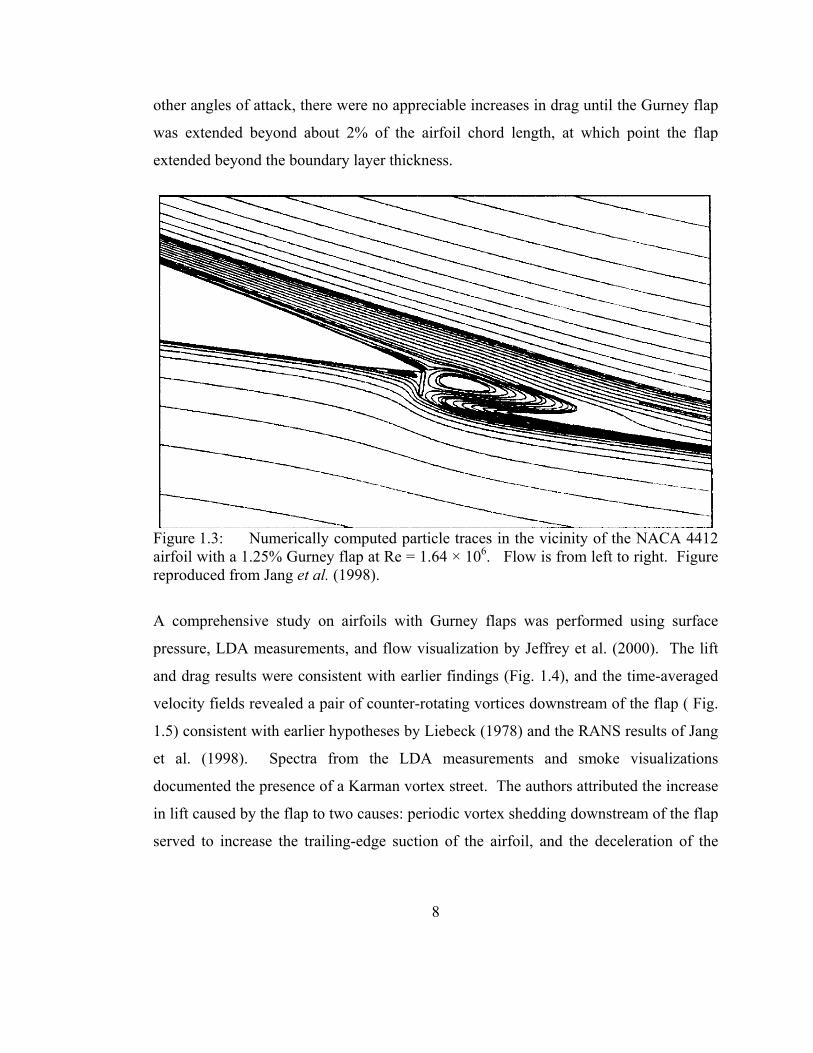
other angles of attack, there were no appreciable increases in drag until the Gurney flap
was extended beyond about 2% of the airfoil chord length, at which point the flap
extended beyond the boundary layer thickness.
Figure 1.3: Numerically computed particle traces in the vicinity of the NACA 4412 airfoil with a 1.25% Gurney flap at Re = 1.64 × 10⁶. Flow is from left to right. Figure reproduced from Jang et al. (1998).
A comprehensive study on airfoils with Gurney flaps was performed using surface
pressure, LDA measurements, and flow visualization by Jeffrey et al. (2000). The lift
and drag results were consistent with earlier findings (Fig. 1.4), and the time-averaged
velocity fields revealed a pair of counter-rotating vortices downstream of the flap ( Fig.
1.5) consistent with earlier hypotheses by Liebeck (1978) and the RANS results of Jang
et al. (1998). Spectra from the LDA measurements and smoke visualizations
documented the presence of a Karman vortex street. The authors attributed the increase
in lift caused by the flap to two causes: periodic vortex shedding downstream of the flap
served to increase the trailing-edge suction of the airfoil, and the deceleration of the
8

flow directly upstream of the flap contributed to a pressure difference acting across the
trailing-edge.
Figure 1.4: CL vs angle of attach and CD vs CL for an Eppler e423 section at Re = 0.75 - 0.89 × 10⁶ as determined by Jeffrey et al. (2000). Figure reproduced from Jeffrey et al. (2000).
Figure 1.5: The time-averaged LDA streamline results of Jeffrey et al. (4% Gurney, α = 0°). Figure reproduced from Jeffrey et al. (2000).
9
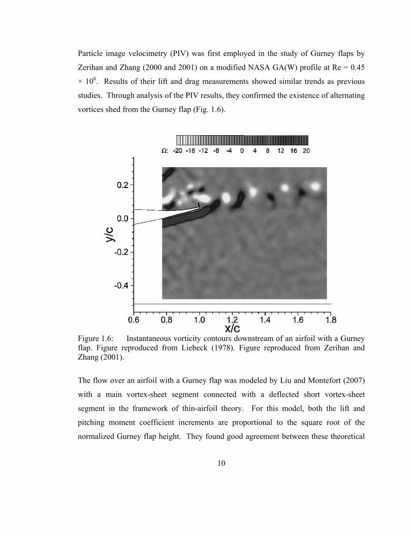
Particle image velocimetry (PIV) was first employed in the study of Gurney flaps by
Zerihan and Zhang (2000 and 2001) on a modified NASA GA(W) profile at Re = 0.45
× 106. Results of their lift and drag measurements showed similar trends as previous
studies. Through analysis of the PIV results, they confirmed the existence of alternating
vortices shed from the Gurney flap (Fig. 1.6).
Figure 1.6: Instantaneous vorticity contours downstream of an airfoil with a Gurney flap. Figure reproduced from Liebeck (1978). Figure reproduced from Zerihan and Zhang (2001).
The flow over an airfoil with a Gurney flap was modeled by Liu and Montefort (2007)
with a main vortex-sheet segment connected with a deflected short vortex-sheet
segment in the framework of thin-airfoil theory. For this model, both the lift and
pitching moment coefficient increments are proportional to the square root of the
normalized Gurney flap height. They found good agreement between these theoretical
10
11
relations and the experimental data of Li et al. (2002), Moyse et al. (2006), Jeffrey et al.
(2000), Storms and Jang (1994), and Jang et al. (1998).
The effect of Gurney flaps at higher Reynolds numbers has also been explored. A study
by Li et al. (2002) included lift, drag, and pressure measurements on a NACA0012
airfoil at a Reynolds number of 2 × 10⁶. This study further confirmed the increase in lift
with slight drag increase for the Gurney flap. Their recommendation was that the
Gurney flap be used on aircraft at moderate to high lift coefficient conditions such as
takeoff and landing, and should be retracted or stowed during low lift coefficient
conditions, such as cruise. The effect of a Gurney flap at higher Reynolds number
where compressibility becomes important was explored through the use of
Compressible Reynolds-averaged Navier-Stokes (RANS) computations employed by
Singh et al. (2007) to predict the flow field around NACA 0011 and NACA 4412
airfoils with Gurney flaps ranging in size from 0.5 to 4% at Mach number of 0.14 and
Reynolds number of 2.2 × 10⁶. Results similar to previous studies were confirmed with
reasonable agreement with available experimental data, in that the lift coefficient and
nose-down pitching moment was increased as compared to the clean airfoil. The drag
penalty increased only slightly except for the 4% flap, which increases the drag more
substantially.
1.2.2.2 Delayed Separation
An important benefit of the implementation of a Gurney flap on an airfoil is the effect
of delayed separation on the suction surface. A study by Neuhart and Pendergraft
(1988) in the NASA Langley 16 × 24 inch water tunnel (the water tunnel was
decommissioned in the late 1990s) at a Reynolds number of 8588 gave valuable
qualitative information on the wake structure of a Gurney flap through visual
observation of dye streaks. The proposed flow structure of Liebeck was generally
confirmed, though the Reynolds number here was substantially smaller (Fig. 1.7). Most
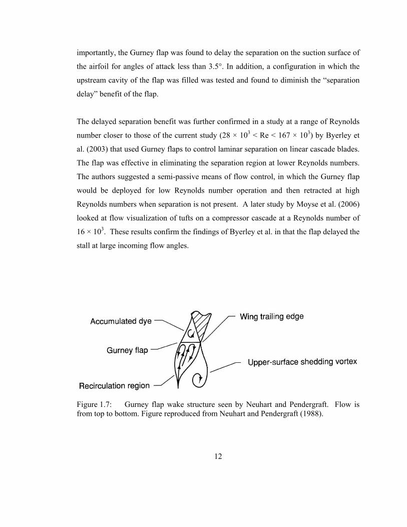
importantly, the Gurney flap was found to delay the separation on the suction surface of
the airfoil for angles of attack less than 3.5°. In addition, a configuration in which the
upstream cavity of the flap was filled was tested and found to diminish the “separation
delay” benefit of the flap.
The delayed separation benefit was further confirmed in a study at a range of Reynolds
number closer to those of the current study (28 × 103 < Re < 167 × 103) by Byerley et
al. (2003) that used Gurney flaps to control laminar separation on linear cascade blades.
The flap was effective in eliminating the separation region at lower Reynolds numbers.
The authors suggested a semi-passive means of flow control, in which the Gurney flap
would be deployed for low Reynolds number operation and then retracted at high
Reynolds numbers when separation is not present. A later study by Moyse et al. (2006)
looked at flow visualization of tufts on a compressor cascade at a Reynolds number of
16 × 103. These results confirm the findings of Byerley et al. in that the flap delayed the
stall at large incoming flow angles.
Figure 1.7: Gurney flap wake structure seen by Neuhart and Pendergraft. Flow is from top to bottom. Figure reproduced from Neuhart and Pendergraft (1988).
12

13
1.2.2.3 Boundary Layer Effects
In addition to the characteristic of delaying the separation point on the suction surface
of an airfoil, is the effect of a Gurney flap on the boundary layer. Several studies have
addressed this issue specifically.
The aim of a study by Giguere et al. (1997) was to find a flow-based scaling for the
optimal Gurney flap height for maximum lift-to-drag performance. The experiment
used a slightly modified LA203A airfoil at Re = 2.5 × 10⁵. They concluded that the
best indicator of proper scaling for the Gurney flap height is the boundary layer
thickness at the trailing edge on the pressure surface of the airfoil at the same angle of
attack without a Gurney flap. For most cases, they found that a Gurney flap height of
1% - 2% was optimal.
At a higher Reynolds number of 2.2 × 10⁶, Myose et al. (1996) at Wichita State
University used a pressure rake to determine the average wake profile of a NACA0011
airfoil. A boundary layer mouse (an array of pitot tubes) was also used to estimate the
boundary layer thickness on the suction surface of the airfoil at 0.9c. Similar to
previous results, they found that the Gurney flap increased the airfoil lift at all angles of
attack, and at low to moderate angles of attack, the Gurney flap increased the drag only
slightly for flaps 2% of the chord length or less. At 0° angle of attack, the boundary
layer thickness on the suction surface was found to be 1.5% of the chord length,
indicating that the 2% Gurney flap extended only slightly into the freestream. At high
angles of attack and thus larger CL, the 2% Gurney flap provided increased lift and
decreased drag. The Gurney flap also had the effect of increasing the nose-down
pitching moment.
The drag begins to increase substantially as the height of the Gurney flap increases
beyond the boundary layer thickness. Gai and Palfrey (2003) used lift and drag

14
measurements and oil flow surface visualization to study a NACA 0012 airfoil with a
5% Gurney flap at 2 × 10⁵. Due to the large height of the Gurney flap, the increase in
drag was found to outweigh the benefit of the increase in lift, resulting in a lower L/D
than the airfoil without the Gurney flap.
1.2.2.4 Flow Control
An interesting application of Gurney flaps is in the area of control, where actuated flaps
are used to increase or decrease the lift on an airfoil locally, in order to affect some
change in the flight path or wake characteristics.
Solovitz and Eaton (2002) experimented with mesoscale trailing-edge actuators in a
static case, which resemble Gurney flaps on a MES05 profile wing at Re = 7.5 × 10⁵.
The aim of the study was to determine if many such actuators attached to an airfoil
trailing edge would allow the localized control of the generated lift. It was found that a
single flap exhibited a spanwise influence at least 10 flap spans away, indicating
considerable nonlocal effects.
Subsequent studies by Solovitz (2002) and Solovitz and Eaton (2004a and 2004b)
looked at dynamically actuated Gurney flaps as a means of controlling UAVs on the
MES05 airfoil with a blunt trailing-edge at Re = 9.0 × 10⁵. The flap could be actuated
at frequencies in excess of 17 Hz (St = 0.0070). Using time- and phase-averaged
particle image velocimetry (PIV) techniques, they were able to analyze the resulting
dynamic flow structure produced in the region around static and dynamically-actuated
Gurney flaps. They found that a dynamically actuated Gurney flap produced a localized
lift response that is linearly dependent on actuated span and is nearly quasi-steady for
dimensionless actuation times (t*act - tU∞/c) near unity because the actuation time was
assumed to be significantly larger than the bluff-body vortex shedding period for the

flaps. They concluded that actuation times near unity are probably practical for real
flight conditions. Overall, they concluded that the devices had many characteristics that
would benefit control design. The MiTEs applied a known lift increment over a fairly
localized region, and the responses of neighboring MiTEs superposed linearly. For
flight conditions, the dynamic response was quasi-steady. Thus, MiTE actuators could
be modeled quite simply in control algorithms. A computational analysis of airfoils
with MiTEs, similar to those studied by Solovitz and Eaton (2002) was performed by
Lee and Kroo (2004). Time-accurate studies were conducted to explore unsteady
effects. The simulation had the flow starting impulsively on a NACA 0012 airfoil with
a 1.5% Gurney flap at Re = 1.5 × 10⁶. Figure 1.8 shows the results, where the lift
coefficient was found to have a high frequency fluctuation which the authors attributed
to vortex shedding.
Figure 1.8: Time history of Cl for an impulsively started NACA0012 airfoil with a 1.5% flap attached. Figure reproduced from Lee and Kroo (2004).
15

16
The study was continued by Matalanis and Eaton (2006) who investigated the use of
MiTEs for wake vortex control with pressure taps and PIV. The experimental study
utilized a modified NACA 0012 with a blunt trailing edge where the actuated Gurney
flap was stowed at an angle of attack of 8.9 degrees. The Reynolds number for the tests
was 3.5 × 10⁵. They found that through dynamic actuation, the trailing wingtip vortex
could be displaced by 0.041 chord lengths in the spanwise direction and 0.016 chord
lengths in the liftwise direction. A subsequent study by Matalanis and Eaton (2007)
suggested that MiTEs can be used to introduce spatial disturbances to a trailing wingtip
vortex in both the spanwise and lift directions depending on the nature of the dynamic
actuation. For cases where relatively large portions of the span are actuated down
(46%), the deflections are greater in the lift direction, whereas for cases where relatively
small portions of the span are actuated down (13%), the deflections are greater in the
spanwise direction. In addition, Matalanis (2007) performed vortex filament
computations that were used to compute the far wake evolution. Results from these
computations showed that the perturbations created by MiTEs could be used to excite a
variety of three-dimensional inviscid vortex instabilities. Tang and Dowell (2007)
studied a dynamically actuated trailing-edge strip that ran the entire span of the airfoil.
The experiments were conducted on a NACA 0012 base airfoil at Re = 3.84 × 10⁵.
They also concluded that the dynamically actuated strip can be a useful tool for active
aerodynamic flow control of a wing.
Trailing wingtip vortices were further studied by Nikolic (2006a and 2006b) who used
flow visualization on a NACA 4412 airfoil with 1.5%, 4%, and 6% Gurney flaps at 0.25
× 106 to investigate the vortex rollup. By fixing long yarn tufts (~ 2.5c) to the trailing
edge of the airfoil 8 mm apart, a qualitative indication of the strength of the trailing
edge vortex could be evaluated by determining a “rollup tightness factor” (RTF). A
downstream tuft grid was also used. It was found that the presence of the flap served to
decrease the strength of the trailing vortex. It was also hypothesized by Nikolic (2006c)
that based on the Helmholtz vortex laws, additional streamwise vortices should exist,

17
that is, the spanwise vortices ought to continue and bend at the tips of the flap and then
extend downstream into the wing wake in the form of trailing vortices.
1.2.2.5 Perturbed Gurney Flaps
In addition to the traditional Gurney flap, several studies have examined the flow affects
of Gurney flaps that have been perturbed in some way in an effort to increase the lift to
drag ratio of the airfoil. The following section discusses several of these investigations.
A variety of Gurney flap shapes (e.g. flaps with slits, holes, wakes stabilizers, etc.)
including a diverging trailing edge which resembles a Gurney flap with the upstream
cavity filled in, were studied by Bechert et al. (2000). The airfoil shape was a HQ17 at
Re = 0.5 – 1.0 × 10⁶. They found that, for the diverging trailing edge, the drag is
decreased, but the lift is also decreased, such that the divergent trailing edge produces
lift more comparable to a smaller standard Gurney flap. Along the same lines, Meyer et
al. (2006) performed experiments and computations on airfoils at Re = 106 with 3D
modifications to Gurney flaps including holes in the flap, slits, and vortex generators at
the top and bottom of the flap. These modifications were capable of reducing the
amount of drag that is produced by a standard Gurney flap by approximately 6%, while
reducing the lift by 4.5%, which improves the lift-to-drag ratio.
A similar study by Traub et al. (2006) performed a parametric study of the dependence
of Gurney flap effects on flap height, porosity, inclination angle, and spacing from the
surface (the flap was specially mounted leaving a gap between the trailing edge and the
Gurney flap) through the use of force balance and pitot-static measurements on a
NACA 0015 with a blunt trailing edge at Re = 0.57 × 10⁶. The data suggested that the
lift augmentation of the flap varies linearly with flap height, porosity and the projected
height of the flap normal to the surface. A following study by Traub and Agarwal

18
(2007) on the same airfoil at similar Reynolds number studied a segmented and “V”
wedge Gurney flap, in which the flap appeared solid when viewed from downstream or
from the side, but exhibited a deviation in the streamwise direction when viewed from
below (alternating Vs and discontinuous rectangles). These results indicated that the V
pattern flap had only a small effect on the lift and drag, whereas the segmented pattern
reduced both lift and drag leading to an increase in lift-to-drag ratio.
Another set of devices that can be thought of as modified Gurney flaps are static
extended trailing edges (SETEs). A SETE is a thin splitting plate mounted at the
trailing edge of an airfoil, but rather than protruding 90° to the chordline, it is mounted
with a small deflection angle (5 - 10°). Its effect is to extend the chord and deflect the
flow toward the pressure side of the airfoil. Liu et al. (2007) studied a NACA 0012
airfoil at Re = 4.74 × 10⁵ with a SETE. Compared with a Gurney flap and a
conventional flap, the SETE generated a larger lift increase at a smaller drag penalty
since it is imbedded in the wake of the main airfoil. For this reason, the authors
suggested that the SETE has a promising potential for improving aircraft cruise flight
efficiency.
1.2.2.6 Specific Applications
The previous sections focused on the characteristics of Gurney flaps specifically. The
following section discusses specific applications in which the benefits of Gurney flaps
may be utilized.
Price (2001), Rhee (2004), Guzel et al., Kinzel et al. (2005), Gerontakos and Lee
(2006), and Lee and Lee (2007) studied the effect of Gurney flaps on oscillating airfoils,
which is important in connection with rotorcraft operations, in which blade vortex
interactions have the potential to cause potentially hazardous rotor vibration. Price

19
examined a NACA 0012 airfoil oscillating at 4.5 Hz over a range of Reynolds numbers
from 0.96 to 1.92 × 10⁵ with and without a Gurney flap and found that the Gurney flap
had the effect of moving the point of laminar separation and onset of transition forward
on the airfoil. Rhee and Guzel et al. performed RANS CFD analysis on an oscillating
VR-12 airfoil, but had difficulties in producing satisfactory quantitative results close to
the experimental data, though qualitatively, the trends were similar. Kinzel et al. used a
CFD solver to investigate the use of miniature trailing-edge effectors (MiTEs) for
rotorcraft applications on an S903 airfoil at Re = 1.0 × 10⁶. They found that MiTEs have
the ability to be used as an active stall control device, and that there does not appear to
be any significant shortcoming of the MiTE’s potential for rotorcraft. Gerontakos and
Lee (2006) investigated a NACA 0012 airfoil at Re = 1.07 × 10⁵ through surface
pressure measurements, and found that the Gurney flap concept was applicable for an
oscillating airfoil in terms of lift and drag, except for the increase in negative pitching
moment which has the potential to promote dynamic stall. They concluded that the
device would be valuable in terms of dynamic actuation and active flow control. The
experiments of Lee and Lee (2007) were performed on a NACA 0015 airfoil at Re =
1.74 × 10⁵ and found that the Gurney flap was effective in increasing the core radius
and circulation of the vortices shed downstream of the flap. Yee et al. (2007)
performed 2D unsteady RANS computations on a NACA 0012 airfoil with Gurney
flaps of heights 0.5, 1, 2, and 4% of the chord at Re = 6.54 × 10⁶ as it applies to
rotorcraft applications. This study confirmed the findings of previous studies and
concluded that it is appropriate to implement the Gurney flap at the outboard of the
rotor blade since the blade stall usually starts from the blade tip region, and that the
implementation of the Gurney flap would greatly improve the figure of merit of the
rotor blade in hovering conditions, since the lift-to-drag ratio is improved.
Gurney flaps have been investigated for use on multi-element wings by Papadakis et al.
(1997), Carrannanto et al. (1998), and Myose et al. (1998). In general, it was found that
the flap was most beneficial when used on the trailing edge of the last wing element.
20
A cooperation between EADS and Airbus in which the feasibility and practical
considerations are investigated in adding miniature trailing-edge devices (Mini-TEDs)
to a commercial jetliner for purposes of adaptive flight control is described by
Lorkowski et al. (2004). The possible benefits of a higher L/D include faster climb in
take-off, improved maneuverability and adaptive stability control in gusty or turbulent
conditions and steeper and slower landing approaches.
Different airfoil planform shapes have also been examined. Wang et al. (2006) studied
the Gurney flap on a swept wing model at Mach numbers ranging from 0.05 to 0.7
through force measurements. The largest increments of the maximum lift coefficient
and maximum lift-to-drag ratio were 16.8 and 24.1%, respectively. They found that the
major factor affecting the efficiency of a Gurney flap in lift enhancement is its
windward (planform) area. Several researchers have performed experimental studies on
the effect of a Gurney flap on a delta wing. See for example, Traub and Galls (1999),
Buchholz and Tso (2000), Li and Wang (2003), and Zhan and Wang (2004). In general,
it was found that the Gurney flap increased the nose-down pitching moment, increased
the drag slightly, and increased the lift. Overall, the lift-to-drag ratio was increased at
moderate to high lift coefficients.
1.3 Objectives and Approach
A summary of the key findings from previous research are:
• Airfoil lift and drag characteristics are sensitively dependent on the chord
Reynolds number for Reynolds numbers less than about 8 × 10⁵.
• There is a transitional regime in the flow over airfoils that exists in the
approximate range of 105 < Re < 106, where the flow transitions from laminar to

21
turbulent across a region containing local separation called a laminar separation
bubble, after which, the flow reattaches to the body as a turbulent boundary
layer.
• Gurney flaps added to airfoils exhibit added lift benefit with minimal drag
penalty over a fairly large range of Reynolds numbers (8.6 × 10³ < Re < 6.5 ×
106), with possible benefits extending beyond this range.
• The presence of a Gurney flap has the effect of delaying separation on the
suction surface of the airfoil.
• Gurney flaps are already in use in some applications and show strong potential
for use in a wide variety of other applications, for example, flow control.
As the literature has shown, the benefits of Gurney flaps have been well documented.
The current study purposes to add to the current research by addressing the topic of the
flow evolution in the region upstream and downstream of a Gurney flap. In addition,
the flow effects at lower Reynolds numbers, in the regime often operated in by UAVs
and MAVs, where the use of Gurney flaps would be particularly useful, have not been
fully addressed. Many questions regarding the specifics of the flow patterns generated
by the Gurney flap still remain.
In the current study, a NACA 0015 airfoil is used, which has large thickness and no
camber, suggesting that this airfoil is not advantageous for use at lower Reynolds
numbers; however, it provides an ideal test case to investigate issues encountered at
lower Reynolds numbers, since the effects are accentuated.
The primary objective of this study is to answer some of the remaining questions to
develop a deeper understanding into the way that the flow around airfoils interacts with
Gurney flaps, and the changes that result.
Answers to the following questions are sought:

22
• What flow structures are induced by the presence of a Gurney flap and how do
they evolve?
• How do angle of attack, Gurney flap height, and Reynolds number affect the
flow structures over airfoils?
• How do angle of attack, Gurney flap height, and Reynolds number affect the
vortex shedding frequencies present in the wake of an airfoil with a Gurney
flap?
• Are the fluid interactions in the upstream cavity of the Gurney flap relevant in
the increase in lift?
• What would be the effect if the upstream cavity were filled-in?
This study quantifies the effects of a Gurney flap on a NACA 0015 airfoil through time-
averaged force measurements, hot film anemometry, high resolution particle image
velocimetry (HRPIV), and time-resolved particle image velocimetry (TRPIV).
Although it is well known that the flaps yield increased lift forces, the mechanisms
behind the increases are still not well understood. HRPIV allows investigation of small
spatial scales in the context of larger flow patterns which are not easily observed or
quantified by other measurement techniques. TRPIV can be used to examine evolving
flow fields in order to observe variations not associated with a “standard” vortex street.
As will be described, an additional shedding mode associated with the recirculation
zone upstream of the flap appears to contribute significantly to the overall airfoil lift.

23
Chapter 2
2 Experimental Apparatus and Methods
2.1 Wind Tunnel Facility
The experiments were conducted in the University of Minnesota Department of
Aerospace Engineering Open Return Wind Tunnel, designed and built by Engineering
Laboratory Design, Inc. (ELD). A drawing of the wind tunnel can be seen in Fig. 2.1.
The open return, blower tunnel has overall dimensions of 11.69m × 2.90m × 3.03m, and
a working section of 2m × 0.6m × 0.6m. Air is drawn through a filtered inlet by a
centrifugal fan driven by a 40hp AC induction motor, where it proceeds through a series
of flow straightening honeycomb meshes and an 8:1 symmetrical contraction into the
working section. The air then exits to the atmosphere through the diffuser which
expands at a 7° angle in the horizontal and vertical directions. A second diffuser was
added since the original drawing as shown in Fig. 2.1; therefore, the actual diffuser
length was 2m. The ductwork is fabricated from a lamination of plastic reinforced
fiberglass and rigid foam. Interior surfaces are glass smooth. Within the test section,
the ceiling and sidewalls are made from 19mm thick clear acrylic. The floor is smooth
MDF board with slots for traversing measurement devices. The freestream velocity in
the test section is continuously variable from 3.5 m/s to 50 m/s, with a velocity variation
less than ± 1% of the mean, and turbulence level based on the streamwise component of
velocity of less than 0.25%.

Figure 2.1: Drawing of the Wind Tunnel (Courtesy ELD Inc. Reprinted with permission).
24

A photo of the wind tunnel inlet filter, diffuser, contraction area, and test section can be
seen in Fig. 2.2.
Figure 2.2: Photo of the wind tunnel.
2.2 Airfoil Characteristics
The coordinate system used throughout the study can be seen in Fig. 2.3, where the
origin is located at the mid span of the airfoil at the chordline trailing edge. As the
angle of attack of the airfoil is changed, the coordinate system remains fixed to the
airfoil trailing edge but does not rotate with the airfoil, so that the positive x-direction
always indicates the direction of the freestream velocity.
25

x
y
z
Figure 2.3: Schematic showing the flow coordinate system.
The airfoil shape chosen for this work was the NACA0015 cross-section, which was
chosen for its simple structure, well understood performance, and large body of existing
experimental data. The NACA0015 airfoil has zero camber, and its maximum thickness
is 15% of the chord at the quarter-chord location. The airfoil was designed in such a
way that the trailing third could be removed and replaced with different trailing edge
shapes. A total of four trailing edge designs were tested. Three trailing edges included
Gurney flaps with heights (h) of 1%, 2%, and 4% of the total chord length (c). The
Gurney flap height (h) was measured from the bottom tip of the flap to the chord line at
the trailing edge (Fig. 2.4). The standard NACA0015 without a Gurney flap is called
the 0% case, to match the nomenclature of the airfoils with Gurney flaps. The
coordinates of the four airfoil shapes can be found in Appendix A.
26

Figure 2.4: Schematic drawing of the airfoil with Gurney flap (not to scale).
The airfoil sections and flap attachments were fabricated in a StratasysTM rapid-
prototype machine at the University of Minnesota Department of Aerospace
Engineering and Mechanics from acrylonitrile butadiene styrene (ABS) polymer. The
airfoils had a span (b) of 304.8 mm and a chord length (c) of 190.5 mm, resulting in an
aspect ratio AR = 1.6. The airfoil body and flap attachments can be seen in Fig. 2.5.
Figure 2.5: Photo of the airfoil test sections.
27

Due to tolerances in the manufacturing process, the actual height of the Gurney flaps
differed slightly from the 1%, 2%, and 4% designations. In addition, the airfoil without
a flap came to a near point at the trailing edge, but did contain finite thickness. The
actual dimensions of the trailing edges are shown in Table 2.1, where the Gurney flap
height is measured from the tip of the flap to the chordline.
Flap Actual (%) Actual (mm)
0% 0.05 0.1
1% 1.00 1.9
2% 1.99 3.8
4% 3.99 7.6
Table 2.1: Actual Gurney flap heights.
In the wind tunnel, the airfoil was mounted to a flat, circular aluminum end plate on one
end by two ¼-20 bolts, as seen in Fig. 2.6.
Figure 2.6: Photo of the 4% flap configuration attached to the aluminum mounting plate.
28
The other end of the airfoil was positioned approximately two millimeters from the
opposite tunnel wall. This was done to mitigate 3D effects on the flow of interest. To
confirm the 2D nature of the flow, tufts of thread were glued to the wing surface, which
showed that the flow was primarily in the downstream direction with no strong
secondary flow structures due to wing tip effects, especially in the center of the airfoil,
where the PIV and hotwire measurements were taken.
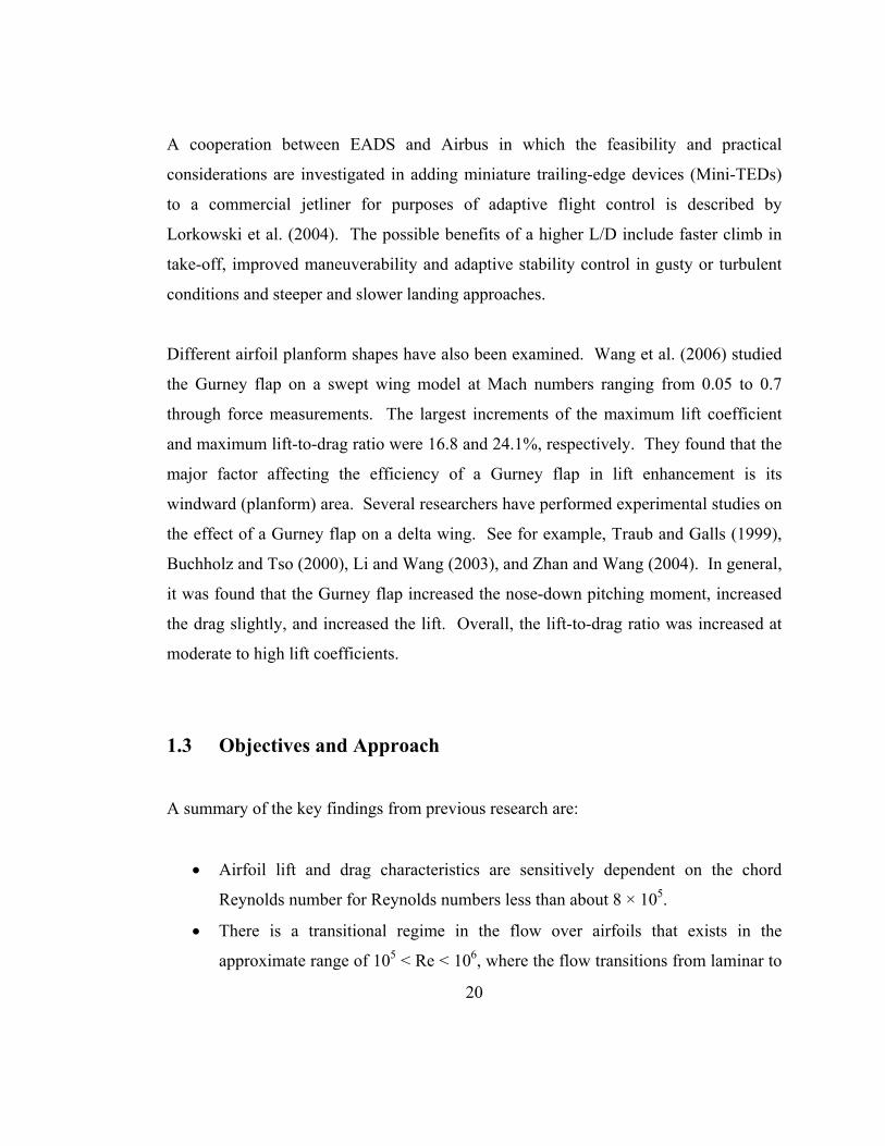
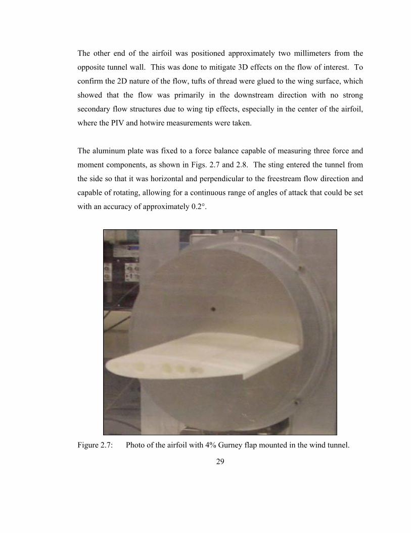
The aluminum plate was fixed to a force balance capable of measuring three force and
moment components, as shown in Figs. 2.7 and 2.8. The sting entered the tunnel from
the side so that it was horizontal and perpendicular to the freestream flow direction and
capable of rotating, allowing for a continuous range of angles of attack that could be set
with an accuracy of approximately 0.2°.
Figure 2.7: Photo of the airfoil with 4% Gurney flap mounted in the wind tunnel.
29
Figure 2.8: Airfoil section mounted in wind tunnel showing the mounting bracket.
In addition to the flapped airfoils, a “filled” flap configuration (4%) was also tested
(Figs. 2.9 and 2.10), in which the upstream cavity of the Gurney flap from the tip to the
point ⅓c from the trailing edge on the pressure side of the airfoil, was filled in. This
arrangement made it possible to determine the direct influence of the upstream
recirculation region on the downstream wake.
30

Figure 2.9: Schematic of the filled-in flap configuration (not to scale).
Figure 2.10: Photo of the filled-in flap configuration.
31

2.3 Freestream Velocity Characteristics
2.3.1 Blockage Effects
Experiments were performed at two wind tunnel motor frequencies: 10.8 Hz and 21.7
Hz. For all experiments, the frequency was set to a constant value, and the tunnel was
allowed to warm up for at least half an hour, and not changed for the duration of the
experiment. Due to blockage effects of the airfoil and the mounting apparatus, the
upstream freestream velocity within the tunnel was not constant for all angles of attack.
The velocity was measured with a hotfilm anemometer at least four chord lengths
upstream of the airfoil. A plot showing the dependence of the freestream velocity on
the angle of attack of the airfoil and mounting apparatus can be seen in Fig. 2.11.
Turbulence intensity, as defined below, is also plotted.
%100.... ×⎟⎠⎞
⎜⎝⎛=
MeanDSIT , (2.1)
Where T.I. is the turbulence intensity, S.D. is the velocity standard deviation, and Mean
is the mean velocity.
0
2
4
6
8
10
12
14
16
18
20
0 5 10 15
Angle of Attack (deg)
Free
stre
am V
eloc
ity (m
/s)
Velocity 10.8 HzTurbulence 10.8 Hz (%)Velocity 21.7 HzTurbulence 21.7 Hz (%)
32
Figure 2.11: Dependence of freestream velocity on angle of attack.
33
Table 2.2 shows the change in Reynolds number as the angle of attack of the airfoil is
changed. Before each run, the current atmospheric pressure was read from the
barometer located on the roof of the mechanical engineering department at the
University of Minnesota along with the lab temperature read from a thermocouple
inside the tunnel. From these quantities, the air density (ρ) was calculated using the
ideal gas law.
The blockage effect was relatively minor, and the Reynolds number remains nearly
constant over the range of angles of attack of interest. Therefore, the two Reynolds
numbers at which data were taken will be referred to as 1.0 × 10⁵ and 2.1 × 10⁵.
10.8 Hz 21.7 Hz
α (°) U∞ (m/s) Re (× 105) U∞ (m/s) Re (× 105)
0 7.951 1.00 16.79 2.12
2 7.891 9.97 16.72 2.11
4 7.852 9.93 16.71 2.11
6 7.863 9.93 16.67 2.10
8 7.822 9.88 16.71 2.10
10 7.809 9.86 16.54 2.08
12 7.748 9.80 16.58 2.08
Table 2.2: Dependence of Freestream velocity and chord Reynolds number on angle of attack.
2.4 Force Balance
Lift measurements were determined through the use of a six-sensor force and moment
balance. Each of these sensors contained a series of internal strain gages, whose output
were converted to six analog voltage signals. These six amplifier outputs were
proportional to the three Cartesian forces and three Cartesian moments that rotated with
the angle of attack of the sting. Prior to each measurement, the zero offset of each
channel was measured by taking 50 measurements over the course of 90 seconds with
the airfoil and mounting apparatus installed, but without flow in the wind tunnel. For
the actual measurements, the wind tunnel was set to the desired speed, allowed to reach
equilibrium, and the balance outputs were sampled 50 times over the course of 90
seconds and averaged. The voltage responses were then converted to forces and
moments.
The lift was the force in the positive y-direction (perpendicular to the freestream flow
direction), as displayed on the coordinate system shown previously in Fig. 2.3. The
data was corrected to account for the finite aspect ratio and the wind tunnel walls, as
described in the following section.
2.4.1 Correction to Infinite Aspect Ratio and Wall Influence
The equations for correcting the data to infinite aspect ratio and for the influence of the
tunnel walls are the same as those used in Jacobs and Anderson (1930) and are based on
the work of Prandtl (1921), Munk (1923, 1925), Munk and Miller (1925), and Glauert
(1923, 1926).
The absolute lift coefficient (CL) was calculated from:
cbULCL 2
21
∞
=ρ
, (2.2)
34

where L is the lift, ρ is the air density, U∞ is the freestream velocity, c is the airfoil
chord length, and b is the airfoil span. In order to correct the data to infinite aspect
ratio, the effective aspect ratio (ARe) is calculated and given by:
( )22
11 Dbe
ARAR−
= , (2.3)
Where AR is the actual aspect ratio of the airfoil and D is the diameter of the wind-
tunnel throat. Since the current study uses a square wind tunnel cross section instead of
a circular cross section, the spanwise distance between the tunnel wall and the endplate
on the airfoil was used for D.
The data is then corrected to account for the closed throat tunnel conditions to free air
using the following relationship:
iT ααα +=0 , (2.4)
Where α0 is the angle of attack of an airfoil with infinite span that would give the same
CL as the airfoil tested in the tunnel, αT is the angle of attack of the airfoil in the tunnel,
and αi is the angle of attack induced on the airfoil in the tunnel by the tunnel walls, and
is given by the following:
( )π
τπ
α 1801 ×+=e
Li AR
C, (2.5)
Where α’s are measured in units of degrees, and τ is a factor correcting the induced
angle of attack to allow for the change from elliptical span loading resulting from the
use of an airfoil of rectangular planform (in this case, τ = 0.11).
35

2.5 Hotfilm Anemometry
A constant temperature anemometer (CTA) was used to obtain velocity measurements
in the region of the airfoils. The CTA principle relies on the cooling effects of a heated
sensor in a flow, which ultimately provides a time series of velocity data that can be
analyzed to determine velocity and time-domain statistics such as power spectra.
2.5.1 Principle of Hotfilm Anemometry
A simple CTA circuit is shown in Fig. 2.12.
Figure 2.12: A simple CTA circuit. (Courtesy TSI Incorporated)
A CTA contains a Wheatstone bridge with a hotwire or hotfilm sensor acting as a
resistor in one of the arms. The sensor is heated by an electric current. An amplifier
balances the bridge by keeping the wire resistance (and temperature) constant, even
though the current passing through the sensor is changing due to the cooling effect of
the flow velocity. The bridge voltage corresponds to the heat transfer of the sensor, and
is a direct measurement of the flow velocity.
36

The measurements conducted in this study utilized a four-channel CTA system
manufactured by TSI Incorporated. The data collection unit was the model IFA300,
and a simple schematic of the circuit is shown in Fig. 2.13. The IFA300 is basically a
Wheatstone bridge with several enhanced features. The first is the SMARTTUNE
feature, which consists of a series of resistors used to balance the bridge. The optimal
configuration of resistors is chosen depending on the experimental setup and the flow
velocity. The stability of the bridge can be monitored with an internal square-wave test
feature. The IFA300 also contains user-selectable gain, offset, low and high-pass
filtering for signal conditioning.
Figure 2.13: Schematic of the IFA300 (Courtesy TSI Incorporated).
2.5.2 Converting Voltage to Effective Velocity
The output of a CTA circuit is a bridge voltage (Eb) corresponding to the effective
velocity. The standard procedure is to define a relationship between output voltage and
velocity. The voltage signal is conditioned to use the full resolution of the A/D
converter:
37

, (2.6) ( ) GainOffsetEE bO ×−=
where EO is the output voltage, and the Gain and Offset are selected such that EO nearly
fills the -5V to +5V input of the A/D. The A/D creates a 12-bit binary count, B, as
follows:
10
)5(4095
+= OE
B . (2.7)
The deconditioned voltage, Eb, is then back-calculated:
( )[ ] OffsetGain
BEb +−×
=54095/10 . (2.8)
The voltage is then corrected for temperature as follows:
( )( )es
csb TT
TTEE
−−
×= , (2.9)
where E is the temperature corrected voltage, Ts is the sensor temperature, Tc is the
ambient temperature during calibration, and Te is the temperature during the
experiment. E is now corrected to be equivalent to the bridge voltage in the calibration
file and in the lookup file.
The basic calibration is a curve fit of the effective velocity, Veff, as a function of the
bridge voltage, E, where:
, (2.10) 432 EDECEBEAKVeff ×+×+×+×+=
Though the King’s Law equation is often used as the calibration curve, in practice, the
fourth-order polynomial has been shown to give results with smaller deviations from the
calibration data points (TSI ThermalPro Manual).
Then density correction is applied as follows:
effc
coreff VPP
V ×=)( , (2.11)
Where Veff(cor) is the density corrected velocity, Pc is the atmospheric pressure during the
calibration, P is the atmospheric pressure during the experiment, and Veff is the effective
38
39
velocity arrived at after the calibration has been applied to the temperature corrected
voltages.
These steps were performed in the ThermalPro software during the calibration and the
data-taking. Typical values of temperature and pressure were 18C and 100 kPa,
respectively.
2.5.3 Anemometer Frequency Response
The closed loop frequency response of a constant temperature anemometer depends on
several factors including the thermal properties of the sensor and the fluid, the overheat
ratio, the temperature coefficient of the sensor, the fluid velocity, the gain of the
amplifier, the resistance of the bridge and the bandwidth of the amplifier (TSI TB5).
The most common method for testing the frequency response of a circuit and sensor is
to introduce an electrical square wave on one side of the bridge and observe the output
on an oscilloscope. The TSI IFA300 has a square wave generator built into the unit.
Square-wave tests were performed on the hotfilm sensors slightly above the maximum
velocity achieved during the experiments. The maximum frequency response was
found to be near 50 kHz, which is well above the maximum frequencies measured
during the experiments.
2.5.4 Hot Film Probes
All of the measurements were made with a TSI model 1210-20 hot film probe which
has a 50.8 μm diameter platinum-coated quartz substrate sensor with a sensing length of
1.02 mm. The distance between the sensor support needles is 1.65 mm. A schematic
of the probe can be seen in Fig. 2.14. An image of the probe can be seen in Fig. 2.15.

Figure 2.14: Model 1210-20 Hotfilm probe schematic. (Courtesy TSI Incorporated)
Figure 2.15: Photo of the model 1210-20 Hotfilm probe.
40
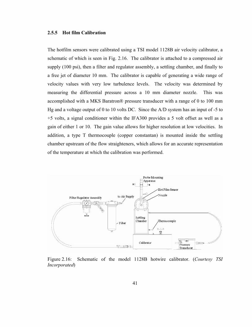
2.5.5 Hot film Calibration
The hotfilm sensors were calibrated using a TSI model 1128B air velocity calibrator, a
schematic of which is seen in Fig. 2.16. The calibrator is attached to a compressed air
supply (100 psi), then a filter and regulator assembly, a settling chamber, and finally to
a free jet of diameter 10 mm. The calibrator is capable of generating a wide range of
velocity values with very low turbulence levels. The velocity was determined by
measuring the differential pressure across a 10 mm diameter nozzle. This was
accomplished with a MKS Baratron® pressure transducer with a range of 0 to 100 mm
Hg and a voltage output of 0 to 10 volts DC. Since the A/D system has an input of -5 to
+5 volts, a signal conditioner within the IFA300 provides a 5 volt offset as well as a
gain of either 1 or 10. The gain value allows for higher resolution at low velocities. In
addition, a type T thermocouple (copper constantan) is mounted inside the settling
chamber upstream of the flow straighteners, which allows for an accurate representation
of the temperature at which the calibration was performed.
Figure 2.16: Schematic of the model 1128B hotwire calibrator. (Courtesy TSI Incorporated)
41

The hotfilm calibrations consisted of 17 points each, with higher point measurement
density at the lower velocities, since the gradient in the calibration curve is steepest for
these points. At each point, 4000 voltage measurements were acquired over a period of
1 second and averaged. A fourth order polynomial was used to fit the data. Several
different probes of the same type were used throughout the testing period. The
calibration curves for the hotfilm probes used can be seen in Fig. 2.17.
1
1.2
1.4
1.6
1.8
2
2.2
2.4
2.6
2.8
3
0 5 10 15 20 25 30 35
Velocity (m/s)
Vol
tage
(V) s/n 45034
s/n 45035s/n 913038s/n 985067
Figure 2.17: Hotfilm probe calibrations.
In order to increase the measurement resolution, a gain and offset were applied to the
signals before being read into the 12-bit PowerDAQ A/D card, in order to take full
advantage of the -5 to +5 voltage range available. A table showing the gain and offset
values used for each probe is shown in Table 2.3.
42

43
Probe s/n Operate Resistance (Ω) Overheat
Ratio
Offset (V) Gain Operating
Temp. (C)
45034 9.12 1.5 1.85 6 250
45035 9.29 1.5 1.74 6 250
913038 9.27 1.5 1.77 6 250
985067 8.96 1.5 1.84 6 250
Table 2.3: Operating resistance, overheat ratio, offset, gain, and operating temperature for the hotfilm probes.
2.5.6 Free Stream Velocity Measurements
Free stream velocity measurements in the wind tunnel were taken at least four chord
lengths upstream of the airfoil for 104 seconds at a sampling rate of 20 kHz, and filtered
at 10 kHz to prevent aliasing. The results were averaged to obtain the mean and
standard deviation.
2.5.7 Shedding Frequency Measurements
Shedding frequencies downstream of the airfoil with and without Gurney flaps were
measured at a distance of 0.7c downstream of the trailing edge. Each hot film
measurement was taken for 104 seconds at a sampling rate of 20 kHz. The
measurements were filtered at 10 kHz to prevent aliasing. Power spectra were
calculated based on the hot film data.

2.6 Particle Image Velocimetry (PIV)
Particle image velocimetry is a technique used to determine the velocity in a plane of a
fluid in motion. The technique is described in great detail by Keane and Adrian (1990
and 1991). It is generally considered a non-invasive measurement technique; however,
in most practical flow situations, small tracer particles must be added to the fluid. PIV
does not measure the fluid velocity directly, but rather the dominant displacement of a
group of tracer, or seed, particles within a small interrogation region by recording their
locations at two known times and performing a cross-correlation. Then using the
fundamental definition of velocity, ttxxtxu ΔΔ= /),(),( rrrr , where is the estimated
local velocity, is the displacement of the tracer particles, and is the time
between recordings, the velocity of the tracers is determined.
),( txu rr
),( txx rrΔ tΔ
Performing PIV measurements on a given flow entails the following steps. A basic
schematic of the PIV setup is shown in Fig. 2.18. Tracer particles that have been added
to the flow are illuminated by a thin sheet of light. A timing device controls the light
source as well as a camera focused on the light sheet. Two exposures are recorded,
either in one image, or in separate images. Through statistical correlation performed
on many small regions throughout the image, the exposures are analyzed to determine
the local flow velocity. Typically the resulting vector field is then post-processed in
order to remove spurious vectors and replace missing vectors with a local mean.
44
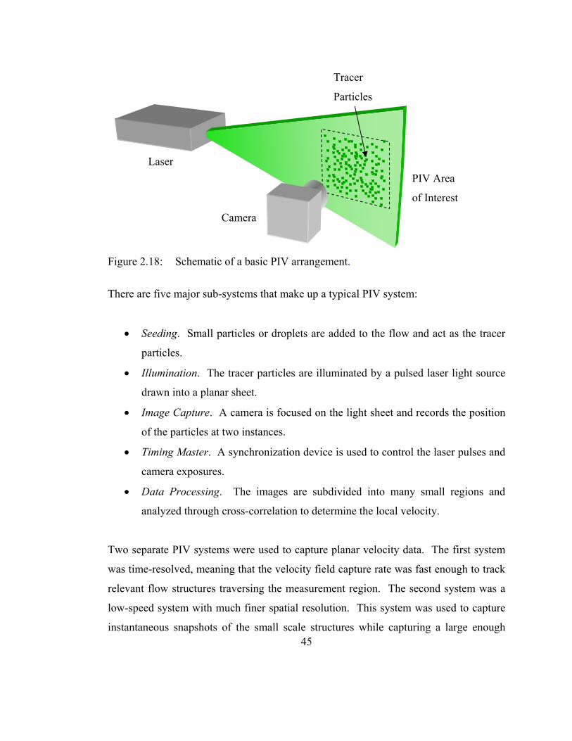
Camera
Laser PIV Area
of Interest
Tracer
Particles
Figure 2.18: Schematic of a basic PIV arrangement.
There are five major sub-systems that make up a typical PIV system:
• Seeding. Small particles or droplets are added to the flow and act as the tracer
particles.
• Illumination. The tracer particles are illuminated by a pulsed laser light source
drawn into a planar sheet.
• Image Capture. A camera is focused on the light sheet and records the position
of the particles at two instances.
• Timing Master. A synchronization device is used to control the laser pulses and
camera exposures.
• Data Processing. The images are subdivided into many small regions and
analyzed through cross-correlation to determine the local velocity.
45
Two separate PIV systems were used to capture planar velocity data. The first system
was time-resolved, meaning that the velocity field capture rate was fast enough to track
relevant flow structures traversing the measurement region. The second system was a
low-speed system with much finer spatial resolution. This system was used to capture
instantaneous snapshots of the small scale structures while capturing a large enough

46
area to understand the relationship to the large flow structures. All PIV data were
generated with the same method of seeding.
2.6.1 Seeding
PIV estimates the velocity of seed, or tracer, particles. It is important that the seed
particles are large enough to be seen by the recording device, but small enough to
follow the local flow velocity which depends on the smallest scales in the flow. A
fairly uniform size distribution is desirable to avoid data drop out or biases in the
measurements. The shape of the particle is important for two reasons, the first is so that
the reaction of the particle to the flow is independent of its orientation, and the second is
so that light scattered off of the particle will appear of uniform intensity no matter the
particle’s orientation. For these reasons, spherical particles are often used.
An additional consideration in the selection of seed particles is the toxicity. Since the
particles will be distributed throughout the flow, and in the case of most airflows,
throughout the laboratory environment, it is important that the particles are non-toxic to
the occupants.
Previous work with PIV has shown that certain liquids can be effectively atomized to
generate droplets adequate as seed particles. In particular, atomized olive oil has
frequently been used to seed airflows for PIV. The advantage of olive oil is that it is
nontoxic and when atomized with a Laskin nozzle, produces droplets with a mean
diameter of approximately 0.9 μm with a standard deviation of 0.63 μm (Thomas and
Butefisch, 1993). Figure 2.19 shows the droplet distribution from a Laskin nozzle used
with olive oil.

Figure 2.19: Measured particle size distribution of olive oil seeding particles generated by a Laskin nozzle particle generator. Reproduced from Thomas and Butefisch (1993).
A TSI model 9307 atomizer was used with olive oil to generate seed particles (fig.
2.20). The reservoir was filled half-full with olive oil, and then compressed air was
forced through the Laskin nozzle located beneath the surface of the oil. Small air
bubbles are produced containing oil droplets. The bubbles rise to the surface and burst,
freeing the oil droplets into the upper part of the chamber. An impactor plate is located
near the top of the inner chamber to block larger particles from exiting. The air and
atomized oil droplets exit the device through an exit orifice at the top.
47

Figure 2.20: Photo (left) and schematic (right) showing the internal components including the impactor plate and the Laskin nozzles of the TSI Model 9307 Oil Droplet Generator (Courtesy TSI Incorporated).
In order to assume that the particles faithfully following the fluid flow, it is necessary to
analyze the time response of an oil droplet. The analysis of Feller and Myers (1976)
was used, in which the time constant of a particle is given by,
g
ppp
dμ
ρτ
18
2
= (2.12)
where the oil droplet density is given by ρp (~ 850 kg/m3), the mean diameter given by
dp (1 μm), and the viscosity of the working fluid, in this case, air, by μg (1.79 × 10⁻⁵
kg/m-s). Therefore, the time response of a 1 μm olive oil droplet in air is approximately
2.6 μs, which corresponds to a frequency of 3.8 × 10⁵ Hz. Olive oil droplets in air will
follow Lagrangian fluctuations in the flow up to 380 kHz within 3 db with an amplitude
error of 37%. Multiplying by the acceleration due to gravity, the settling velocity of
48

approximately 26 μm/s is attained, which is negligible compared with the dominant
velocities in these experiments.
Olive oil droplets were introduced into the wind tunnel by way of a rubber hose
attached to the output port of the droplet generator. The other end of the hose was
placed inside the filtered inlet of the blower. The droplets were sufficiently mixed with
the input air as they passed through the blower and through the flow straighteners.
Within the center of the test section of the tunnel, the droplets formed a quite uniform
distribution. The droplet density was observed to be less near the walls; however, this
was not an issue since PIV measurements were not taken in these locations.
2.6.2 Illumination
The illumination source for the low-speed high-resolution PIV measurements was an
Ultra PIV-120 manufactured by Big Sky Lasers, Inc. The dual-head Nd:YAG laser
produced 120 mJ per pulse at 532 nm with a pulse duration of 12 ns and exit beam
diameter of 6 mm. A photograph of the laser can be seen in Fig. 2.21.
Figure 2.21: Laser used for high resolution PIV mounted to the top of the wind tunnel with light sheet optics and mirror.
49
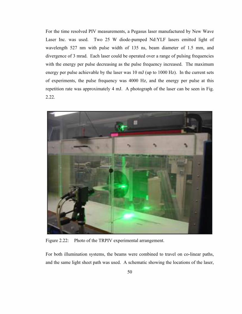
For the time resolved PIV measurements, a Pegasus laser manufactured by New Wave
Laser Inc. was used. Two 25 W diode-pumped Nd:YLF lasers emitted light of
wavelength 527 nm with pulse width of 135 ns, beam diameter of 1.5 mm, and
divergence of 3 mrad. Each laser could be operated over a range of pulsing frequencies
with the energy per pulse decreasing as the pulse frequency increased. The maximum
energy per pulse achievable by the laser was 10 mJ (up to 1000 Hz). In the current sets
of experiments, the pulse frequency was 4000 Hz, and the energy per pulse at this
repetition rate was approximately 4 mJ. A photograph of the laser can be seen in Fig.
2.22.
Figure 2.22: Photo of the TRPIV experimental arrangement.
For both illumination systems, the beams were combined to travel on co-linear paths,
and the same light sheet path was used. A schematic showing the locations of the laser,
50

laser sheet path, and camera can be seen in Fig. 2.23. The laser head was mounted
rigidly to the top of the wind tunnel. Light sheet optics (Fig. 2.24) were mounted
directly to the front of the laser at the exit of the beam. The first component was a -25
mm cylindrical lens which served to expand the circular beam into a sheet. The beam
then passed through a 500 mm spherical lens which focused the beam so that the
thinnest portion of the light sheet was located approximately at the center of the
measurement region. The beam then intersected a mirror placed at 45° from vertical, so
that the light sheet was reflected downward and entered the wind tunnel through the top
Plexiglas surface. At the measurement region waist, the light sheet thickness was
approximately 750 μm for the high-resolution data, and approximately 1 mm for the
time-resolved data.
Figure 2.23: Schematic of the PIV arrangement, including the locations of the laser, laser sheet path, and camera in relation to the PIV area of interest.
51

Figure 2.24: Schematic representation of the laser light sheet optics.
2.6.3 Image Capture
High resolution digital image sequences of the laser light scattered from olive oil
droplets in the plane of the laser sheet were acquired by a 12-bit CCD camera
manufactured by TSI Incorporated (PowerView 11MP) at a rate of 1 fps (0.5 Hz PIV
capture rate). The camera can be seen in Fig. 2.25. The resolution of the camera was
4008 × 2672 pixels, with an individual pixel size of 9 μm square and peak quantum
efficiency of 50%. A 105 mm Nikon lens at f# 5.6 was used along with two 14 mm
extension rings to provide a very high magnification ratio of nearly 1:1. For this reason,
the field of view was approximately the same as the CCD size (36.07 × 24.05 mm).
52

Figure 2.25: TSI PowerView 11MP Camera used for high resolution PIV measurements (Courtesy TSI Incorporated).
To capture PIV data very close to the airfoil surface, it was necessary to have part of the
airfoil within the field of view of the camera where the illuminating laser sheet
produced very harsh reflections. In order to reduce reflections, rhodamine B paint was
applied to the airfoil, and two 532 ± 10 nm band-pass filters were attached to the camera
lens. Rhodamine dye in the paint is excited by the 532nm (green) laser light and emits
between 560 nm and 600 nm (orange) light, which is subsequently filtered out by the
camera filters. The fluorescent paint reduced the reflections substantially and was
applied several times per day in order to maintain its fluorescent properties. The PIV
setup, as well as the effect of the rhodamine B paint can be seen in Fig. 2.26.
53

Figure 2.26: PIV setup with orange-fluorescent rhodamine paint visible on the airfoil surface.
Figure 2.27 is an actual camera image showing the effect of the rhodamine paint. In
this figure, the left side of the airfoil surface has the paint; the right side does not have
paint. The pink areas indicate saturated pixels.
Saturated pixels in PIV are detrimental in two distinct ways. The first is that when a
pixel is saturated with photons, the actual intensity received by the pixel is not known.
In this case, it could be slightly above the maximum distinguishable intensity of the
pixel, or it could be significantly higher. In the latter case, it is quite possible that the
CCD array of the camera could be damaged due to the extreme intensity of the signal.
In general, saturated pixels should be avoided to ensure that the camera is not damaged.
The second reason is that saturated pixels often lead to “bleeding,” where pixels
adjacent to the saturated ones are flooded with intensity, typically in the direction that 54

the intensity data is read out of the CCD array. In this case, data is lost, not only in the
saturated pixel, but also in neighboring pixels. This effect can be seen slightly in Fig.
2.27, where near the left portion of the saturated (pink) region, bleeding is seen
occurring down toward the bottom of the image.
Figure 2.27: Rhodamine Paint on an airfoil with laser on. Paint has been applied on the left side, but not on the right side.
For the time resolved image capture, digital image sequences were acquired from a 10-
bit CMOS high speed camera manufactured by Photron Inc. at rates of 2000 frames per
second and 4000 frames per second which correspond to velocity field capture rates of
1000 Hz and 2000 Hz, respectively (Fig. 2.28). The pixel size was 17 microns. At 2000
frames per second the camera resolution was 1024 by 1024 pixels, and at 4000 frames
per second with pixel resolution was 1024 by 512 pixels. Higher frequencies were
attempted with this configuration, but the laser illumination energy was too low to
produce meaningful results. A 50 mm Nikon lens was used with the aperture setting of
55

f#1.4. The full field of view ranged from (123 mm)2 to (141 mm)2 depending on the
distance to the measurement region which changed slightly for the various flap
configurations.
Figure 2.28: Photron APX camera used for time-resolved PIV measurements.
2.6.4 Timing Synchronization
The camera frames and laser pulses were synchronized with a TSI model 610035
synchronizer (Fig. 2.29) with 1 ns resolution, which was controlled by INSIGHT3G
software from TSI Incorporated. The pulses from each laser were timed to straddle
neighboring camera frames in order to produce images suitable for PIV cross-
correlation (Figs. 2.30 and 2.31). The time between frame-straddled laser pulses (Δt)
56

was set such that a suitable displacement of particles from the first frame to the next,
was achieved.
Figure 2.29: TSI 610035 LaserPulse Synchronizer (Courtesy TSI Incorporated).
Figure 2.30: Timing diagram for TRPIV image acquisition at 4000 Hz (Δt = 20 μs).
57

Figure 2.31: Timing diagram for HRPIV image acquisition (Δt = 5 μs).
A suitable displacement is defined as a displacement that is small enough that the
images of seed particles do not leave the user-defined cross-correlation interrogation
region either horizontally, vertically, or out of the laser sheet representing the out of
plane component, and large enough to minimize the uncertainties in the calculated
displacements, upon which the velocity is based.
The Δt values used for the various experiments are shown in Table 2.4.
Exp U∞
(m/s)
Δt
(μs)
Particle Disp
at U∞
(pixels)
Pixel
Size
(μm)
Lens
FL
(mm)
Magnification
(μm/pixel)
Mag
HRPIV 16.8 5 8 9 105 9.88 – 9.95 1:1.1
HRPIV 7.95 5 4 9 105 9.88 – 9.95 1:1.1
HRPIV LE 16.8 5 8 9 105 11.40 – 11.44 1:1.3
HRPIV LE 7.95 5 4 9 105 11.40 – 11.44 1:1.3
TRPIV 16.8 20 4 17 50 41.83 – 48.51 1:2.9
Table 2.4: Significant parameters used in each of the PIV experiments.
58
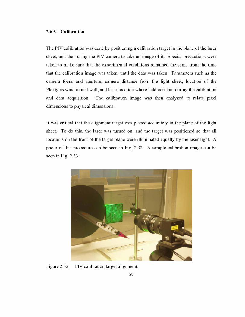
2.6.5 Calibration
The PIV calibration was done by positioning a calibration target in the plane of the laser
sheet, and then using the PIV camera to take an image of it. Special precautions were
taken to make sure that the experimental conditions remained the same from the time
that the calibration image was taken, until the data was taken. Parameters such as the
camera focus and aperture, camera distance from the light sheet, location of the
Plexiglas wind tunnel wall, and laser location where held constant during the calibration
and data acquisition. The calibration image was then analyzed to relate pixel
dimensions to physical dimensions.
It was critical that the alignment target was placed accurately in the plane of the light
sheet. To do this, the laser was turned on, and the target was positioned so that all
locations on the front of the target plane were illuminated equally by the laser light. A
photo of this procedure can be seen in Fig. 2.32. A sample calibration image can be
seen in Fig. 2.33.
Figure 2.32: PIV calibration target alignment.
59

Figure 2.33: Sample calibration image. Dot spacing is 2.5mm.
2.6.6 PIV Processing
For each case 1000 TRPIV velocity fields, and 50 HRPIV velocity fields were acquired.
TSI software, INSIGHT 3G, was used to process the data. Cross-correlation processing
of PIV images can be broken down into the following steps:
• Image pre-processing
• Interrogation and cross-correlation
• Vector validation
These steps are discussed in detail in this section.
2.6.6.1 Image Pre-Processing
For both the high resolution and time resolved PIV measurements, image preprocessing
was performed. The preprocessing came in the form of a background subtraction of the
minimum intensity (Fig. 2.34). Two sets of raw images (corresponding with Frame A
and Frame B) were conditioned independently before vector processing by first 60
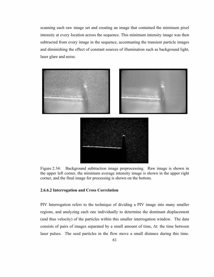
scanning each raw image set and creating an image that contained the minimum pixel
intensity at every location across the sequence. This minimum intensity image was then
subtracted from every image in the sequence, accentuating the transient particle images
and diminishing the effect of constant sources of illumination such as background light,
laser glare and noise.
Figure 2.34: Background subtraction image preprocessing. Raw image is shown in the upper left corner, the minimum average intensity image is shown in the upper right corner, and the final image for processing is shown on the bottom.
2.6.6.2 Interrogation and Cross Correlation
PIV Interrogation refers to the technique of dividing a PIV image into many smaller
regions, and analyzing each one individually to determine the dominant displacement
(and thus velocity) of the particles within this smaller interrogation window. The data
consists of pairs of images separated by a small amount of time, Δt: the time between
laser pulses. The seed particles in the flow move a small distance during this time. 61
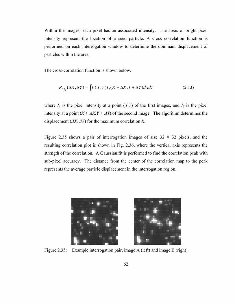
Within the images, each pixel has an associated intensity. The areas of bright pixel
intensity represent the location of a seed particle. A cross correlation function is
performed on each interrogation window to determine the dominant displacement of
particles within the area.
The cross-correlation function is shown below.
dXdYYYXXIYXIYXR II ),(),(),( 2121Δ+Δ+=ΔΔ ∫ (2.13)
where I1 is the pixel intensity at a point (X,Y) of the first images, and I2 is the pixel
intensity at a point (X + ΔX,Y + ΔY) of the second image. The algorithm determines the
displacement (ΔX, ΔY) for the maximum correlation R.
Figure 2.35 shows a pair of interrogation images of size 32 × 32 pixels, and the
resulting correlation plot is shown in Fig. 2.36, where the vertical axis represents the
strength of the correlation. A Gaussian fit is performed to find the correlation peak with
sub-pixel accuracy. The distance from the center of the correlation map to the peak
represents the average particle displacement in the interrogation region.
Figure 2.35: Example interrogation pair, image A (left) and image B (right).
62

Figure 2.36: Correlation map achieved from images shown in Fig. 2.35.
2.6.6.3 CDIC Deformation Method
For the PIV data from both the TRPIV and the HRPIV, a more advanced algorithm was
used to accelerate the correlation calculation, as well as increase the accuracy with
which the displacements were determined. The central difference image correction
(CDIC) algorithm was developed by Wereley and Gui (2003) and involves the dynamic
deformation of the interrogation spots to achieve the highest possible correlation. This
is done by deforming the interrogation regions to allow for both translation of the
particle windows as well as deformations, such as rotation or shear. This technique is
typically done in several iterations, so that the amount of deformation for the final pass
is determined by examination of the neighboring vector displacements. The
interrogation window is then offset at its corners by the prescribed distance.
Due to the differences in the images from the TRPIV to the HRPIV, the specifics of the
CDIC method were altered slightly for the two cases and are discussed in the next
paragraphs.
63

64
2.6.6.4 Time Resolved PIV
For the TRPIV data, a starting interrogation region of 32 × 32 pixels and a final
interrogation region of 16 × 16 pixels were used. which corresponds to a spatial
resolution of 1.1 mm square for the (141 mm)2 field. The interrogation regions were
overlapped by 50%. This processing scheme yielded 97% or higher valid vectors in
each field.
2.6.6.5 High Resolution PIV
For each HRPIV run, 50 PIV velocity fields were captured. The starting spot size was
64 × 64 pixels, and the final interrogation spot size was 32 × 32 pixels, which
corresponds to a spatial resolution of between 320 and 360 μm depending on the exact
magnification, which varied slightly for each case. The interrogation regions were
overlapped by 50%. This processing scheme provided 99% or higher valid vectors.
2.6.6.6 Vector Validation
Several validation schemes were used to remove spurious vectors and replace missing
vectors.
Peak-to-Noise Ratio. The average particle displacement throughout an interrogation
region is determined by finding the highest peak intensity in the correlation map. The
second highest peak is a noise peak caused by the random pairing of images from
different particles. The ratio of the displacement peak height to the noise peak height is
a determination of how much the displacement peak stands out above the noise. Low
peak-to-noise ratios indicate less confidence that the selected peak is the correct peak.
For this reason, vectors determined from correlation spots with a peak-to-noise ratio of
less than 1.5 were removed and not considered valid.

65
Local Median Test. In addition to the peak-to-noise ratio test, a local median test was
also applied to the vector fields. In this step, the velocity components of a given vector
are compared against the value of a reference vector. The reference vector in this case
is the median value of all the vectors in the surrounding 3 × 3 neighborhood (8 vectors
total). A tolerance of 25% of the freestream velocity was applied as the maximum
allowable difference between the current vector and its reference vector.
Missing Vector Replacement. After the spurious vectors were removed in the
previous two steps, the missing vectors were replaced with the mean value of all the
vectors in the 3 × 3 neighborhood. In all the PIV experiments presented the number of
valid vectors, those passing both the peak-to-noise ratio and the local median test, was
97% or greater.
Low Pass Spatial Filter. As a final step, a low pass spatial filter was applied to the
vector field to eliminate the effects of high frequency noise in the fields. This was done
by applying a Gaussian weighting function to each vector, altering its velocity
magnitude and direction based on the behavior of vectors in a local 3 × 3 neighborhood.
This step altered the data only minimally, but increased the visibility of higher order
structures in the flow substantially, such as vortices.
2.7 Uncertainty
2.7.1 Lift Coefficient Uncertainty
The force balance was used primarily to measure the lift on the wing. The absolute
value of the lift was not as important as the repeatability of the experiments, since the
primary use of the data was to compare the differences in lift for several airfoil
configurations. There were many sources of uncertainty in the lift coefficient;

therefore, the repeatability of the measurements was determined through analysis of the
deviation of the results for the symmetric airfoil from zero lift at an angle of attack of
zero. A linear interpolation of the data for the symmetric (NACA0015) airfoil reveals a
lift coefficient at zero angle of attack of 0.033. This configuration is expected to
produce a zero lift coefficient; therefore, the uncertainty is on the order of 4.1% of the
maximum lift coefficient measured.
In order to examine the absolute lift coefficient values, a comparison with previous data
is performed. Figure 2.37 shows a comparison of the absolute lift coefficient (CL) vs.
angle of attack (α0) for a NACA0015 airfoil measured by Jacobs and Sherman (1937) at
Reynolds numbers of 166,000 and 331,000, as well as results from the current work
where the Reynolds number was 210,000. There is good agreement between the two
studies, suggesting that the current experimental setup is satisfactory in offering
comparable results to previously gathered data.
0
0.2
0.4
0.6
0.8
1
1.2
-5 0 5 10 15
Angle of Attack (deg)
Lift
Coe
ffic
ient
Jacobs and Sherman (1937) Re = 331,000Current Study Re = 210,000Jacobs and Sherman (1937) Re = 166,000
Figure 2.37: Comparison of data from the current study with those acquired in the NACA facility (Jacobs and Sherman (1937)). All data are corrected to infinite span and free air.
66

67
2.7.2 Hot film Anemometry Uncertainty
Uncertainties in the velocity measurements resulted mainly from calibrator uncertainty,
calibration curve fitting, flow unsteadiness in the wind tunnel, and the resolution of the
voltage measurements. Commercially available anemometers such as the IFA300 have
low drift, low noise, and good repeatability, so these factors do not add significantly to
the uncertainty in comparison with other error sources, and were neglected. The
uncertainty analysis performed here was similar to that in Finn (2005).
The uncertainty in the calibrator can be attributed to two main sources. The first is a
constant contribution through the full range of velocities. The second source is a
relative standard contribution which varies from point to point and can be expressed as
a percentage of the mean value. The TSI model 1128B calibrator is considered a good
dedicated calibrator with thought put into the design to mitigate uncertainty effects.
Therefore, for the velocity ranges used, the constant uncertainty due to the calibrator
was estimated at ±0.02 m/s, and the relative standard contribution was ±1%.
Uncertainty arising from the calibration curve fit was also considered. It is stochastic in
nature and the relative standard uncertainty was estimated at ±0.5%.
Uncertainty due to flow unsteadiness in the wind tunnel was ± 1% of the freestream
velocity as stated by the tunnel manufacturer.
The resolution of the voltage was determined by the accuracy of the data acquisition
board, which was 12-bit over a range of ±5 V. The resolution was equal to ½ of the
smallest bit value, which gave:

VbitsVwV 00122.0
210
21
12 ±=⎟⎠⎞
⎜⎝⎛±= (2.14)
Then, the resolution uncertainty of the velocity was negligible (~ 0.1%) and given by:
0.0028 m/s (2.15) =VRw ,
Uncertainty can also arise from atmospheric conditions which may vary from the time
of the calibration to the time of the measurements. Since the data was corrected for
changes in temperature and pressure according to the equations discussed previously,
this uncertainty is considered negligible.
The net uncertainty in the hot film measurements resulted mainly from the uncertainty
in the calibrator, calibration curve fitting, the flow unsteadiness in the wind tunnel, and
the resolution of the A/D conversion. Combining these sources resulted in a net
uncertainty in the hot film measurements of ±2.5%.
2.7.3 Particle Image Velocimetry Uncertainty
PIV measurements determined the time-resolved 2D velocity flow field in the region
surrounding the airfoil trailing edge in the vicinity of the Gurney flap. The critical
information gleaned from these results was used to document the difference between the
flow structure for the flapped and unflapped airfoil, as well as to determine the effect of
angle of attack. Thus, the PIV data is presented in terms of the average velocity field
over a number of samples in order to examine absolute velocity information, and in
terms of instantaneous velocity measurements for the purpose of comparing trends in
velocity information as it changed with time, angle of attack, and Gurney flap height.
These trends are determined through analysis of instantaneous velocity and vorticity
fields to determine the way in which flow structures (regions of high or low velocity
68

69
and vortices) interact and evolve. For the instantaneous velocity fields, the absolute
velocity measurement is of less importance than the relative velocity as it compares to
other configurations. For this reason, the absolute uncertainty analysis is performed
only for the averaged velocity fields, and the uncertainty in the instantaneous velocity
fields is estimated based on the uncertainty of the PIV displacement algorithm.
In addition, since the emphasis was on measuring and comparing results from the
different configurations, only sources of uncertainty that would cause differences
between the various cases were considered. Bias errors that affected all datasets in the
same way, such as geometric uncertainty in the wing shape were irrelevant, and were
not considered.
The primary sources of uncertainty were spatial resolution, calibration uncertainty, and
spatial displacement algorithm accuracy. The uncertainty associated with temporal
variations in the laser pulse synchronization is several orders of magnitude smaller and
is neglected (Adrian 1997). In PIV, the spatial resolution is determined by the size of
the interrogation spot. Of course, this requires several assumptions; namely, that the
particles within the interrogation region are equally-spaced and all have a uniform
displacement. The correlation method derives an average displacement for all particles
in the interrogation region, so uncertainty arises from this assumption. For the current
measurements, the square interrogation regions were either 16 or 32 pixels on a side,
which corresponds to physical units of approximately 1mm (TRPIV) or 360 μm
(HRPIV). Thus, if velocity fluctuations with spatial scales smaller than these values,
they will not be resolved. The calibration uncertainty was a bias effect, and was
estimated at ±0.5% based on how well the target was aligned with the laser light sheet.
The spatial displacement accuracy of the CDIC method of Wereley and Gui (2003) used
here was found to be ±0.08 pixels (16 × 16 pixel spot size) and ±0.06 pixels (32 × 32
pixel spot size) as long as the particles images were at least 2 pixels. For the data
gathered here, the particle image sizes range from 2.5 to 10 pixels. This results in an

uncertainty in the displacement of ±2% for the TRPIV data and ±0.75% for the HRPIV
data. Combining all of these effects, the absolute uncertainty in the velocities (u/U∞,
v/U∞) was ±2.5% for the TRPIV and ±1.25% for the HRPIV. Note that very close to
the airfoil surface, where the velocity is close to zero, the percentage is higher.
The vorticity was defined as:
xv
yu
∂∂
−∂∂
=ω (2.16)
This was determined using second-order finite differencing:
1,1,
1,1,
,1,1
,1,1
−+
−+
−+
−+
−
−−
−
−=
jiji
jiji
jiji
jiji
xxvv
yyuu
ω (2.17)
The overall uncertainty in vorticity involves variations in velocity and spatial location.
The uncertainty in spatial location was negligible compared to the uncertainty in
velocity. Each of the velocities in the equation contributed to the overall uncertainty.
Therefore, the overall uncertainty in vorticity (ωc/U∞) was 5% (TRPIV) and 2.5%
(HRPIV).
70

71
Chapter 3
3 Results and Discussion: Force Balance and Flow
Visualization
Force balance measurements and flow visualization results are presented in this chapter.
The force balance was used to determine the lift on the airfoil and the effect of the
Gurney flap height and the airfoil angle of attack. Tufts glued to the airfoil surface
were used in the flow visualization to gather information on the locations of separation
on the airfoil with and without a Gurney flap and at varying angles of attack and
Reynolds number.
3.1 Force Balance Measurements
Force balance measurement results for four Gurney flap heights at a Reynolds number
of Rec = 2.1 × 10⁵ are presented. Lift coefficients, corrected to infinite aspect ratio and
for the influence of the tunnel walls, were computed at different angles of attack and
compared. Resulting plots are used to provide insight into the effect of the Gurney flap
height on the generated lift.
3.1.1 Effect of Gurney Flaps on Lift
Figure 3.1 shows the absolute lift coefficient (CL = L/½ρU∞2cb) versus angle of attack
for the NACA0015 airfoil as well as airfoils with 1%, 2%, and 4% Gurney flaps in the
linear regime of the lift curve. The shape of the lift curve versus angle of attack remains
nearly identical and nearly linear for airfoils with Gurney flaps as compared to the
control airfoil without a Gurney flap; however, CL increases by an average of 0.09 for

the airfoil with a 1% Gurney flap, by 0.21 for the airfoil with a 2% flap, and by 0.36 for
the airfoil with a 4% flap. These trends and the overall curve shapes are consistent with
the findings of Wadcock (1987) and Jeffrey et al. (2000).
0
0.2
0.4
0.6
0.8
1
1.2
-4 -2 0 2 4 6 8 10
Angle of Attack (deg)
Lift
Coe
ffic
ient
4% Gurney2% Gurney1% GurneyNACA0015
Figure 3.1: CL vs. α for airfoils with Gurney flaps of height 0% (blue), 1% (red), 2% (green), and 4% (orange) at Re = 2.1 × 10⁵.
3.1.2 Effect of Filled In Gurney Flap on Lift
In addition to the three flapped cases, a “filled in” airfoil was also tested. This airfoil
shape consisted of the 4% flapped airfoil with the upstream cavity of the airfoil filled in
flush up to a point ⅓c upstream of the trailing edge. This case, shown in Fig. 3.2, shows
an increase in lift coefficient of approximately 0.16, which is slightly less than the 2%
flap case; this result seems reasonable since the rear point of the camber line for the
closed airfoil, which is similar to an airfoil with a diverging trailing edge, is effectively
the same as for the 2% flap, though the camber lines themselves are not the same. This 72

result is consistent with the findings of Bechert et al. (2000). By comparing the 4% flap
and the closed flap, it is seen that only part of the lift increment can be explained by the
mean deflection of streamlines around an asymmetric shape. The remaining increase in
lift coefficient must be a direct result of the flow characteristics in the upstream cavity.
0
0.2
0.4
0.6
0.8
1
1.2
-4 -2 0 2 4 6 8 10
Angle of Attack (deg)
Lift
Coe
ffic
ient
4% Gurney2% Gurney4% Gurney Filled
Figure 3.2: CL vs. α for airfoils with 4% Gurney flaps with an open upstream cavity (orange) and closed upstream cavity (blue). The airfoil with 2% flap is shown in red for comparison. Re = 2.1 × 10⁵.
3.2 Tuft Flow Visualization
3.2.1 Suction Surface Visualization
Tufts of fine white thread were glued to the airfoil surface in order to provide a
qualitative measure of the location of the trailing edge separation point for various
73

74
Reynolds numbers and angles of attack. The Gurney flaps could be installed in either
direction relative to the tufted surface (flap directed up or down), and both the pressure
and suction surfaces of the airfoil were visualized. Visualizations were performed at
two Reynolds numbers: Rec = 1.0 × 10⁵ and Rec = 2.1 × 10⁵, and the angle of attack
was varied from α = 0° up to and including the angle of full-stall, in increments of 1°.
The angles of attack in this and subsequent sections are not corrected for infinite aspect
ratio and wind tunnel wall effects, to allow for a more direct comparison.
The presence of the Gurney flap on the NACA0015 did not appear to change the stall
angle of attack significantly with this resolution; however, the exact point of stall was
difficult to determine visually, and previous work (see Neuhart and Pendergraft (1988),
Moyse et al. (1998) or Jeffrey et al. (2000), for example) has shown that the presence of
a Gurney flap typically decreases the stall angle on the order of 1° to 3° depending on
flap height.
Figures 3.3 and 3.4 show the tuft visualization at the low Reynolds number (Rec = 1.0 ×
105) with and without the 4% Gurney flap at α = 0°, 10°, 12°, and 14°. In Fig. 3.3 (no
Gurney flap), it can be seen that the flow remains laminar on the suction surface up to
and including the α = 10° case. At the α = 12° case, general flow unsteadiness,
separation, and the onset of turbulence can be seen near the center span of the airfoil
closer to the trailing edge which is evidenced by the flapping of individual tufts that are
not oriented in the freestream direction. It is clear from the bottom plot that at this
Reynolds number, separation has occurred and the airfoil is stalled at α = 14°. Figure
3.4 shows the same setup as Fig. 3.3, the only difference is the presence of the 4%
Gurney flap. The view is still of the suction surface, so the flap is not visible from this
direction. The visualizations look similar to the cases in Fig. 3.3, where the flow
appears laminar at α = 0° and α = 10°, and some separation becomes apparent at α =
12°. In the α = 14° visualization, the airfoil is stalled.
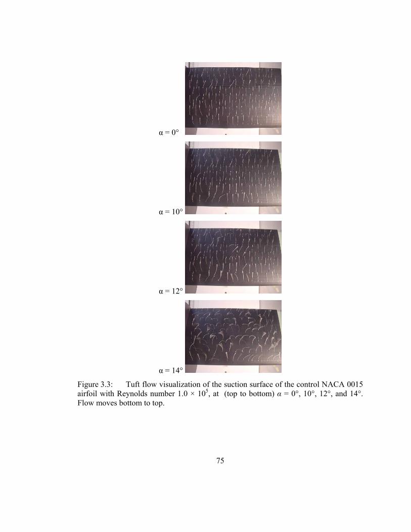
α = 0°
α = 10°
α = 12°
α = 14°
Figure 3.3: Tuft flow visualization of the suction surface of the control NACA 0015 airfoil with Reynolds number 1.0 × 10⁵, at (top to bottom) α = 0°, 10°, 12°, and 14°. Flow moves bottom to top.
75
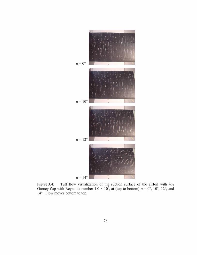
α = 0°
α = 10°
α = 12°
α = 14°
Figure 3.4: Tuft flow visualization of the suction surface of the airfoil with 4% Gurney flap with Reynolds number 1.0 × 10⁵, at (top to bottom) α = 0°, 10°, 12°, and 14°. Flow moves bottom to top.
76

77
Figures 3.5 and 3.6 show the visualization at the higher Reynolds number (Rec = 2.1 ×
105), with and without the 4% Gurney flap at α = 0°, 10°, 13°, 15° and 17°. For both
cases, the stall appears to have occurred at α = 17°.
In Fig. 3.5, the top three visualizations (α = 0°, 10°, and 13°) reveal relatively laminar
flow across the airfoil surface in the freestream direction. At α = 15°, flow separation
near the trailing edge, and the onset of turbulence are apparent. At α = 17°, the flow is
fully separated, and the airfoil is stalled.
Figure 3.6 shows the same setup as Fig. 3.5, with the addition of the 4% Gurney flap.
Again, the flap is not visible in this view of the suction surface. Similar to Fig. 3.5, the
top three visualizations (α = 0°, 10°, and 13°) reveal relatively laminar flow across the
airfoil surface in the freestream direction. At α = 15°, flow separation near the trailing
edge is apparent, and at α = 17°, the airfoil is fully stalled.
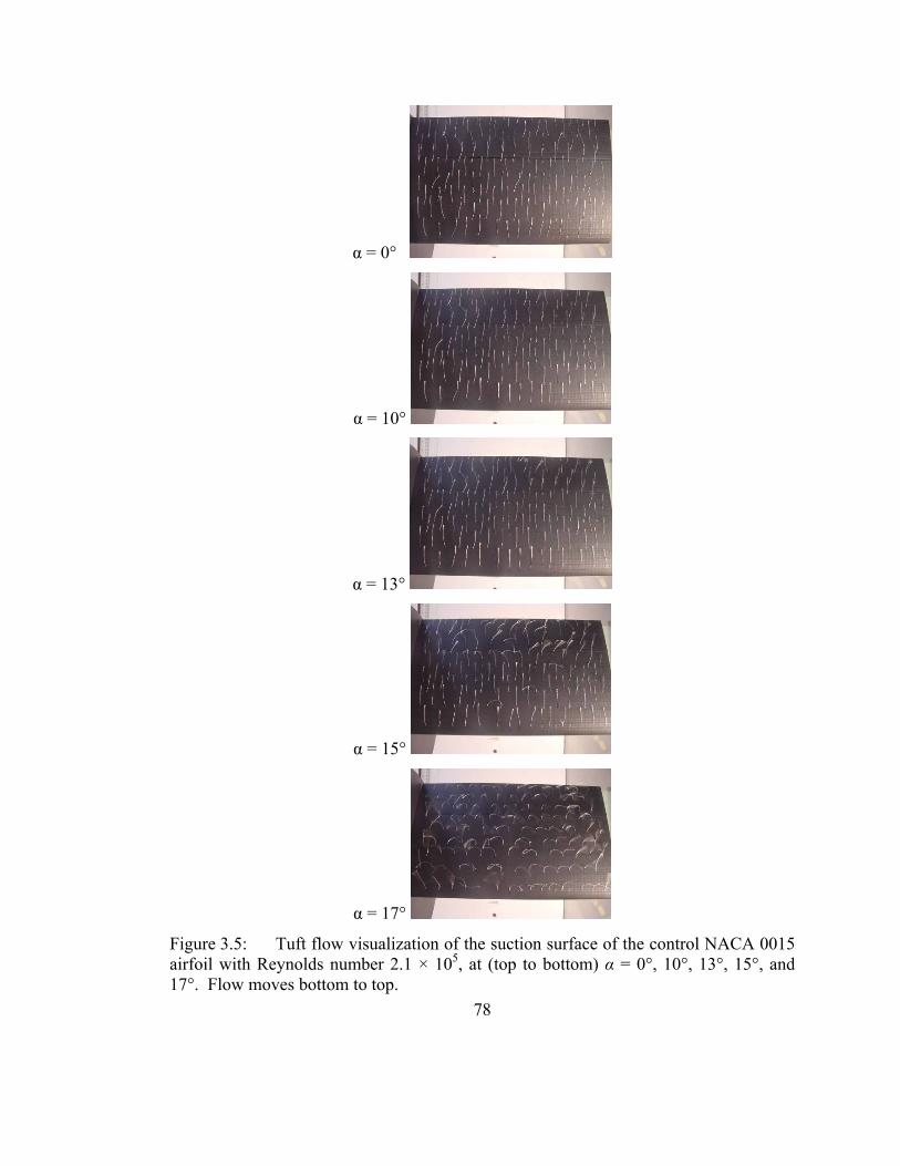
α = 0°
α = 10°
α = 13°
α = 15°
α = 17°
Figure 3.5: Tuft flow visualization of the suction surface of the control NACA 0015 airfoil with Reynolds number 2.1 × 10⁵, at (top to bottom) α = 0°, 10°, 13°, 15°, and 17°. Flow moves bottom to top.
78

α = 0°
α = 10°
α = 13°
α = 15°
α = 17°
79
Figure 3.6: Tuft flow visualization of the suction surface of the airfoil with 4% Gurney flap with Reynolds number 2.1 × 10⁵, at (top to bottom) α = 0°, 10°, 13°, 15°, and 17°. Flow moves bottom to top.

3.2.2 Pressure Surface Visualization
An interesting phenomenon was seen on the pressure surface of the airfoil as the angle
of attack was increased. As expected, no separation was observed on the pressure
surface for the no-flap case. By contrast, the separation zone upstream of the 4%
Gurney flap increased in size with increasing angle of attack. Figure 3.7 shows the
pressure surface for the 4% flap at Rec = 1.0 × 10⁵ for α = 0° and α = 8°. The red
dashed line indicates the approximate location of the boundary between attached and
separated flow. Separation is evident from the tuft tips which are blurred in separated
zones. This trend was confirmed based upon multiple observations of this effect.
Figure 3.7: Comparison of separation regions on pressure surface of the airfoil with a 4% Gurney flap at α = 0° (left) and 8° (right) at Rec = 1.0 × 10⁵. Flow moves bottom to top.
80

81
Chapter 4
4 Results and Discussion: Velocity Measurements
Time-averaged and results for the high resolution PIV datasets are presented in this
chapter. The time-averaged data gives detailed flow insights into the overall effect of
the Gurney flap which is useful for evaluating other measured quantities such as lift and
drag. In the next chapter, instantaneous vector fields are presented to provide a
comprehensive view of the transient flow structures in the region near the Gurney flap.
The freestream velocity values from the PIV data agreed well with the hot film
measurements of the freestream velocity in the wind tunnel. Note that all quantities
presented in this chapter are normalized using the freestream velocity (U∞) and the
airfoil chord length (c). Average velocity fields were computed from fifty independent
high resolution PIV fields. Average velocity fields generated from time-resolved PIV
data are an average of 1000 PIV fields. The origin is located on the airfoil chordline at
the trailing edge, as defined previously. The axes do not rotate with angle of attack.
4.1 Time-Averaged Trailing Edge
Contours of time-averaged streamwise velocity overlaid with streamlines are presented
in Fig. 4.1 (Re = 1.0 × 10⁵) and Fig. 4.2 (Re = 2.1 × 10⁵) for the airfoil without a
Gurney flap at α = 0° and α = 8°. Every tenth vector is shown in the horizontal
direction, and every other vector is shown in the vertical direction. The area shown in
white is the airfoil, and no data were obtained in the black areas which were blocked
from the illuminating laser light.

82
In the average field at the lower Reynolds number (Fig. 4.1), the α = 0° case (top)
reveals a small separation zone near x/c = -0.12 upstream of the trailing edge (indicated
by a circle in the figure). A close-up view of this separation zone (not shown) reveals
an area of flow reversal. Besides this feature, the plot reveals a fairly narrow wake,
with streamlines closely following the surface of the airfoil and coming together at the
trailing edge. The α = 8° case (bottom) reveals a larger recirculation zone characterized
by backwards streamlines that extends from upstream of the trailing edge near x/c = -
0.13 to downstream of the trailing edge near x/c = 0.04. The flow remains attached
along the suction surface. The trailing wake is deflected downward as expected. These
features suggest that laminar separation bubbles are forming due to the adverse pressure
gradient located downstream of the ¼ chord (thickest) point on the airfoil. In the α = 8°
case, the recirculation zone extends beyond the trailing edge, suggesting that the
laminar separation zones are forming and being convected downstream.
At the higher Reynolds number (Fig. 4.2), the streamlines stay attached to the airfoil in
both the α = 0° (top) and α = 8° (bottom) cases, though the boundary layer thickness on
the suction (upper) surface shows a slight increase, and the streamlines are deflected
significantly downward for the α = 8° case, which is what causes the increase in lift as
angle of attack increases and the total circulation around the airfoil increases.
This difference in flow patterns near the trailing edge between Figs. 4.1 and 4.2 indicate
the significant effect that Reynolds number can have on the trailing edge dynamics.

Figure 4.1: Average streamwise velocity on the 0% Gurney flap at Re = 1.0 × 10⁵ for α = 0° (top) and α = 8° (bottom).
83

Figure 4.2: Average streamwise velocity on the 0% Gurney flap at Re = 2.1 × 10⁵ for α = 0° (top) and α = 8° (bottom).
84

85
Similar results are presented in Figs. 4.3 and 4.4 for the 4% Gurney flap at Reynolds
numbers of 1.0 × 10⁵ (Fig. 4.3) and 2.1 × 10⁵ (Fig. 4.4) for α = 0° and α = 8°. The
shape of the streamlines in the downstream wake closely matches those that were
captured with the more coarsely resolved high-speed PIV (Troolin et al. 2006a).
The α = 0° case at low Reynolds number (Fig. 4.3 top) reveals a pair of counter rotating
vortices directly downstream of the flap, which are present for both angles of attack and
both Reynolds numbers. Downstream of the counter rotating vortices, the wake
streamlines are deflected downward as compared to the airfoil without the flap. In
addition, a recirculation zone is present directly upstream of the flap on the pressure
surface of the airfoil. The size of this recirculation zone increases for α = 8° (Fig. 4.3
bottom). The boundary layer along the top surface of the airfoil also increases in
thickness for the higher angle of attack, which is to be expected.
For the higher Reynolds number case (Fig. 4.4), the trends are similar. The counter
rotating vortices are still present downstream of the flap, and the recirculation zone still
exists upstream of the flap, though both of these features are shorter in the streamwise
direction than for the lower Reynolds number case. The boundary layer on the upper
surface is also significantly thinner than in the lower Reynolds number case. These
results are consistent with what would be expected as the Reynolds number is increased.
The boundary layer decreases in thickness, the upstream recirculation zone decreases in
spatial length and thickness, and the downstream wake becomes thinner.

Figure 4.3: Average streamwise velocity on the 4% Gurney flap at Re = 1.0 × 10⁵ for α = 0° (top) and α = 8° (bottom).
86

Figure 4.4: Average streamwise velocity on the 4% Gurney flap at Re = 2.1 × 10⁵ for α = 0° (top) and α = 8° (bottom).
87

88
Three trends can be noted from the previous plots. First, the area of decreased
streamwise velocity directly upstream of the Gurney flap increases in length as the
angle of attack increases from α = 0° to α = 8°. This trend, which is consistent with the
tuft visualization results, is very clear for the lower Re case (Fig. 4.3) but less clear for
the higher Re case (Fig. 4.4). Second, the average separated zone upstream of the flap
decreases in size with increasing Reynolds number, particularly at α = 8°. Third, the
zone of recirculating fluid downstream of the flap decreases in streamwise length as the
angle of attack is increased for Re = 1.0 × 10⁵ (Fig. 4.3), and increases in streamwise
length as the angle of attack is increased for Re = 2.1 × 10⁵ (Fig. 4.4). This is directly
related to the upstream recirculation zone. For the lower Reynolds number case at α =
8°, the upstream recirculation zone is much longer so that the streamlines outside this
zone are straight and directed nearly parallel to the chordline. The streamlines are
drawn easily into the downstream wake leading to a shorter recirculation zone. By
contrast, in the higher Reynolds number case, the streamlines outside the upstream
recirculation zone are diverted strongly by the flap so that they are directed downward
as they pass the flap. They then undergo far greater curvature downstream of the flap
before closing off the downstream recirculation zone. The shorter downstream
recirculation zone seen in Fig. 4.3 for Re = 1.0 × 10⁵ and α = 8° (bottom) is associated
with increased downward curvature of the suction-side streamlines, which must result in
a net increase in the circulation, and thus lift compared with the α = 0° case, as was
verified by force balance results in chapter 3. These results agree well with the time-
averaged velocity fields determined by Jeffrey et al. (2000) and others (see Jang et al.
1998 and Solovitz and Eaton 2004a and b).
Similar data is presented in Figs. 4.5 and 4.6 for the 4% Gurney flap with the upstream
cavity open (Fig. 4.5) and filled in (Fig. 4.6) at Reynolds number of 2.1 × 10⁵ for α =
0° and α = 8°. The main difference is that these data were obtained by averaging 1000
of the time-resolved PIV vector fields.

89
Note that the open flap (Fig. 4.5 top) has a similar average wake appearance as the
filled-in flap for the α = 0° case (Fig. 4.6 top), in that the downstream wake envelops
the counter rotating vortices and appears to close up downstream of the airfoil at a
similar position (x/c = 0.05). However, after the streamlines come together for the open
flap, they have a definite downward deflection. In Fig. 4.5 (top), the deflection angle of
the streamlines at x/c = 0.12 is approximately 9.5°, whereas, for the filled-in case, the
streamlines come together and maintain a deflection of approximately 1° at the same
downstream location. This finding is consistent with the force balance measurements
discussed in chapter 3, where the airfoil with the upstream cavity filled-in revealed less
benefit in terms of the increase in lift (see Fig. 3.2). When the upstream cavity is filled
in, the total circulation on the airfoil decreases, and thus the lift decreases.
The differences increase for the α = 8° case. The shape of the averaged counter rotating
vortices is strikingly different. For the open case (Fig. 4.5 bottom), the two vortices are
approximately the same size spatially, though the clockwise (upper) vortex is shifted
closer to the Gurney flap than the counter-clockwise (lower) vortex. In the filled flap
case (Fig. 4.6 bottom), the two vortices are very different in size. The clockwise vortex
is much larger than the other, and further downstream, the streamlines come together in
an almost horizontal trajectory. The boundary layer on the upper surface of the airfoil
also appears approximately twice as thick for the airfoil with the filled-in flap as
compared to the open flap at this Reynolds number. The deflection angles of the
streamlines at x/c = 0.12 are approximately 12° and 1.5° for the open (Fig. 4.5 bottom)
and closed (Fig. 4.6 bottom) cases, respectively.
Neuhart and Pendergraft (1988) found that separation on the suction surface occurred
earlier (closer to the leading edge) for an airfoil geometry with a filled-in Gurney flap at
Rec = 8588. This suggests that the existence of greater streamline curvature around the
Gurney flap on the pressure side of the airfoil may be a key factor in the increased lift.
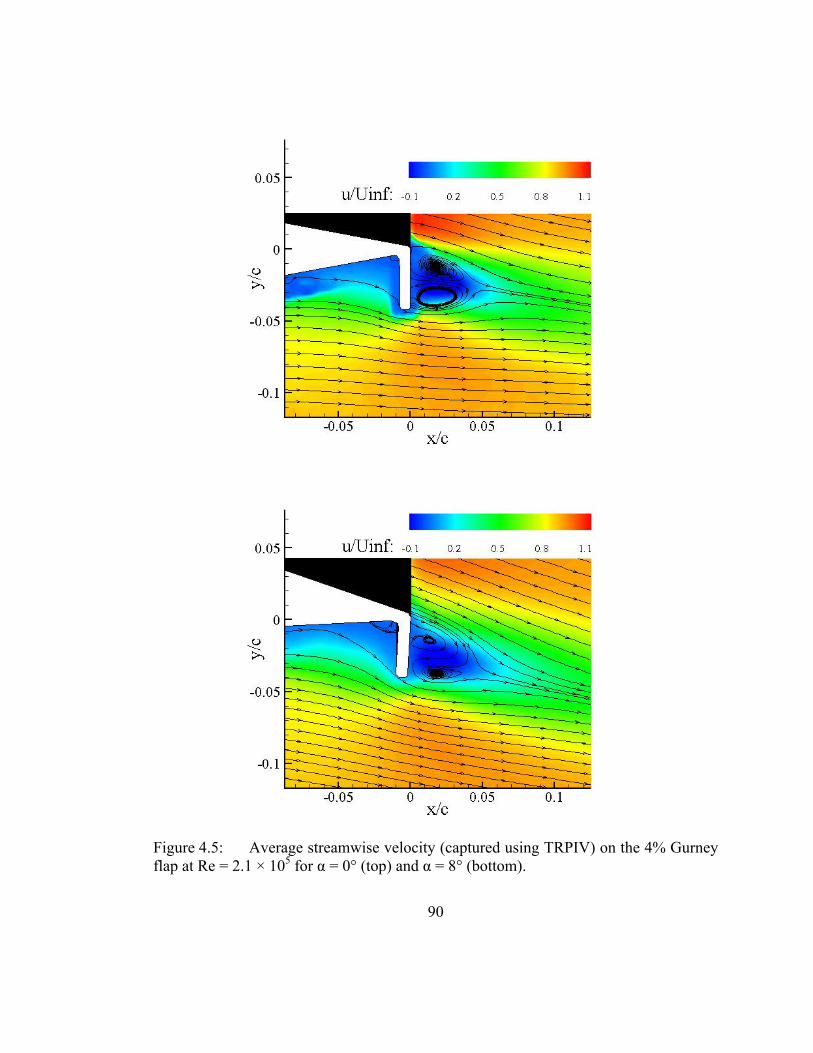
Figure 4.5: Average streamwise velocity (captured using TRPIV) on the 4% Gurney flap at Re = 2.1 × 10⁵ for α = 0° (top) and α = 8° (bottom).
90
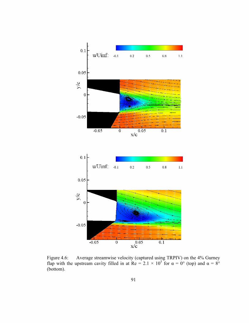
Figure 4.6: Average streamwise velocity (captured using TRPIV) on the 4% Gurney flap with the upstream cavity filled in at Re = 2.1 × 10⁵ for α = 0° (top) and α = 8° (bottom).
91
92
Similar trends in α and Re variation are seen for the 1% and 2% Gurney flaps, which are
shown in Appendix B.
4.2 Time-Averaged Leading Edge
Next, the velocity pattern near the leading edge is examined in order to investigate the
affect the presence of a Gurney flap has on the location of the leading edge stagnation
point. The following plots consist of average PIV measurements taken at the airfoil
leading edge. As in previous plots, the origin is located on the airfoil chordline at the
trailing edge. Again, the results from fifty independent fields were averaged to obtain
the plots which are normalized by the freestream velocity U∞. Every tenth vector is
shown in the horizontal direction, and every other vector is shown in the vertical
direction. The area shown in white is the airfoil, and no data were obtained in the black
areas which were blocked from the illuminating laser light.
Contours of time-averaged streamwise velocity overlaid with streamlines are presented
in Figs. 4.7 and 4.8 for the 0% Gurney flap airfoil at Reynolds numbers of 1.0 × 10⁵
(Fig. 4.7) and 2.1 × 10⁵ (Fig. 4.8) for α = 0° and α = 8°. The same quantities are plotted
in Figs. 4.9 and 4.10 for the 4% Gurney flap at the two Reynolds numbers.
At Re = 1.0 × 10⁵ and α = 0° (Fig. 4.7, top), the streamlines indicate a stagnation point
located precisely at the leading edge and flow acceleration along the pressure surface.
Since the airfoil is symmetric in this case, the flow acceleration on the suction surface
must follow a similar trend. For the α = 8° case (Fig. 4.7, bottom), the stagnation point
shifts downward toward the pressure surface of the airfoil, and the flow acceleration
along the pressure surface occurs over a longer spatial distance. A small patch of high
velocity (red) is seen above the stagnation point on the suction surface, indicating that
the flow accelerates much more quickly over the suction surface.

93
The trends are similar for the higher Reynolds number cases (Fig. 4.8), as would be
expected.
For both Reynolds numbers, the velocity fields are very similar in characteristics. For
the case of the airfoil without a Gurney flap at α = 0° (Figs. 4.7 and 4.8, top), the
stagnation streamline 0.09c upstream of the leading edge intersects y/c very close to
zero, as would be expected. For the case of the 4% Gurney flap at α = 0° (Figs. 4.9 and
4.9, top), the stagnation streamline 0.09c upstream of the leading edge intersects y/c at
approximately -0.008, revealing that the presence of the Gurney flap has the effect of
shifting the forward stagnation point on the leading edge of the airfoil toward the
pressure surface.
The effect is also seen for α = 8° with and without a flap. In Fig. 4.7 and 4.8 (bottom),
where the airfoil does not have a Gurney flap, the stagnation streamline intersects a
point 0.09c downstream of the leading edge near y/c = 0.095. For the case of the airfoil
with the 4% Gurney flap (Figs. 4.9 and 4.10, bottom), the stagnation streamline
intersects at y/c = 0.085.
This effect was also observable, but to a lesser degree for the 1% and 2% Gurney flaps,
which are shown in Appendix B.

Figure 4.7: Average of 50 PIV fields at the airfoil leading edge at Rec = 1.0 × 10⁵ for the 0% Gurney flap at α = 0° (top) and α = 8° (bottom). Color contours represent normalized streamwise velocity.
94
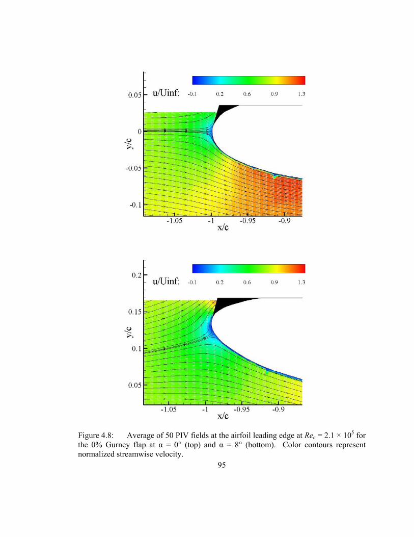
Figure 4.8: Average of 50 PIV fields at the airfoil leading edge at Rec = 2.1 × 10⁵ for the 0% Gurney flap at α = 0° (top) and α = 8° (bottom). Color contours represent normalized streamwise velocity.
95

Figure 4.9: Average of 50 PIV fields at the airfoil leading edge at Rec = 1.0 × 10⁵ for the 4% Gurney flap at α = 0° (top) and α = 8° (bottom). Color contours represent normalized streamwise velocity.
96

Figure 4.10: Average of 50 PIV fields at the airfoil leading edge at Rec = 2.1 × 10⁵ for the 4% Gurney flap at α = 0° (top) and α = 8° (bottom). Color contours represent normalized streamwise velocity.
97

98
Chapter 5
5 Results and Discussion: Time Resolved PIV
Results
The time-averaged data in the previous chapter was presented as a means of putting the
global effect of the Gurney flap into perspective. This chapter focuses on the
instantaneous vector fields which provide time resolved information allowing the
analysis of the temporal evolution of structures around the Gurney flap and the
interactions among them.
5.1 Instantaneous PIV Measurements – No Gurney Flap
Vortex shedding occurs downstream of trailing edges that support separating shear
layers, and the resulting interaction forms the well-known Kármán vortex street. The
Gurney flap acts as a bluff body that produces vortex shedding, but its asymmetry
yields asymmetries in the wake pattern. Of particular interest in this study was the
nature and path of the vortices as they formed and convected downstream. The method
used to study this phenomenon is the analysis of time-resolved velocity fields. All of
the time-resolved velocity sequences presented in this chapter were captured at 4000 Hz
(8000 camera frames per second). The high resolution velocity fields were not time-
resolved, and thus, nominal sequences are shown in order to highlight details of the
instantaneous velocity fields. The normalized quantities shown in the velocity fields are
the y-component of velocity (v/U∞), subsequently referred to as “normal velocity”,
vorticity (ωc/U∞), and two-dimensional swirl strength (λ2Dc/U∞) as defined by Adrian et
al. (2000). In the plots, λ2D, a positive scalar quantity, is given a sign indicating the
direction of the corresponding vorticity at that location.
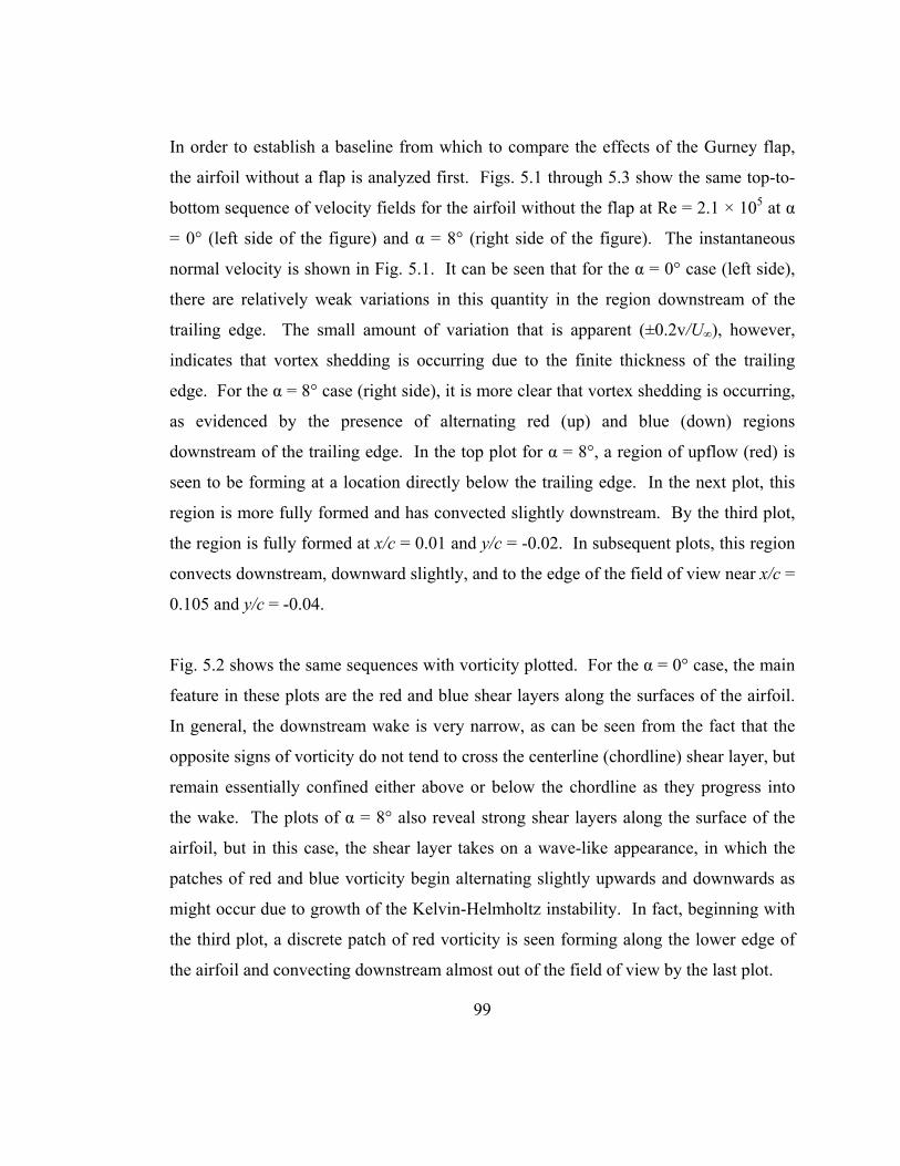
99
In order to establish a baseline from which to compare the effects of the Gurney flap,
the airfoil without a flap is analyzed first. Figs. 5.1 through 5.3 show the same top-to-
bottom sequence of velocity fields for the airfoil without the flap at Re = 2.1 × 10⁵ at α
= 0° (left side of the figure) and α = 8° (right side of the figure). The instantaneous
normal velocity is shown in Fig. 5.1. It can be seen that for the α = 0° case (left side),
there are relatively weak variations in this quantity in the region downstream of the
trailing edge. The small amount of variation that is apparent (±0.2v/U∞), however,
indicates that vortex shedding is occurring due to the finite thickness of the trailing
edge. For the α = 8° case (right side), it is more clear that vortex shedding is occurring,
as evidenced by the presence of alternating red (up) and blue (down) regions
downstream of the trailing edge. In the top plot for α = 8°, a region of upflow (red) is
seen to be forming at a location directly below the trailing edge. In the next plot, this
region is more fully formed and has convected slightly downstream. By the third plot,
the region is fully formed at x/c = 0.01 and y/c = -0.02. In subsequent plots, this region
convects downstream, downward slightly, and to the edge of the field of view near x/c =
0.105 and y/c = -0.04.
Fig. 5.2 shows the same sequences with vorticity plotted. For the α = 0° case, the main
feature in these plots are the red and blue shear layers along the surfaces of the airfoil.
In general, the downstream wake is very narrow, as can be seen from the fact that the
opposite signs of vorticity do not tend to cross the centerline (chordline) shear layer, but
remain essentially confined either above or below the chordline as they progress into
the wake. The plots of α = 8° also reveal strong shear layers along the surface of the
airfoil, but in this case, the shear layer takes on a wave-like appearance, in which the
patches of red and blue vorticity begin alternating slightly upwards and downwards as
might occur due to growth of the Kelvin-Helmholtz instability. In fact, beginning with
the third plot, a discrete patch of red vorticity is seen forming along the lower edge of
the airfoil and convecting downstream almost out of the field of view by the last plot.

100
Fig. 5.3 shows the sequence with two-dimensional swirl plotted. This quantity
identifies swirling, as opposed to shearing, motion; thus, the shear layers present in the
vorticity plots are minimized, and vortex cores are highlighted here. Note that for the α
= 0° case (left), there is very little coloration indicating the presence of vortex cores.
Only a small red vortex is seen in the top frame along the airfoil surface just below the
trailing edge. In the subsequent frames, it separates from the airfoil and begins to
propagate downstream, moving approximately x/c = 0.015 from frame to frame. The α
= 8° case (right) confirms the existence of a vortex core in the positions noted above for
vorticity. In the top plot at x/c = -0.015, a small patch of red is seen along the lower
surface of the airfoil. In subsequent plots, this vortex core progresses downstream,
separating from the airfoil surface in the third plot, and by the last plot, ending up at x/c
= 0.1.

Figure 5.1: Normal velocity (v/U∞) downstream of the airfoil without a Gurney flap at Re = 2.1 × 10⁵ and α = 0° (left) and α = 8° (right).
101

Figure 5.2: Vorticity (ωc/U∞) downstream of the airfoil without a Gurney flap at Re = 2.1 × 10⁵ and α = 0° (left) and α = 8° (right).
102

Figure 5.3: Swirl (λ2Dc/U∞) downstream of the airfoil without a Gurney flap at Re = 2.1 × 10⁵ and α = 0° (left) and α = 8° (right).
Figure 5.4 displays instantaneous plots of the high resolution PIV data, showing
streamlines overlaid on λ2D for the α = 0° case at Re = 2.1 × 10⁵. The streamlines in
103

plots B and C show significant curvature at the airfoil trailing edge indicative of slight
vortex shedding. The trends are similar to the time-resolved data, where some small
vortex cores are seen, but in general, the streamlines are parallel and do not exhibit
large variations in the y-direction downstream of the trailing edge.
Figure 5.4: Instantaneous plots of swirl (λ2Dc/U∞) downstream of the airfoil without a Gurney flap at α = 0° and Re = 2.1 × 10⁵.
Figure 5.5 is similar to Fig. 5.4, with α = 8°. The streamlines downstream of the trailing
edge do not show large variations in the y-direction. The presence of more regions of
red and blue located near the airfoil surface indicate small vortex cores developing in
the boundary layer and shed into the downstream wake. The trends are similar to the
time-resolved data, where some small vortex cores are seen, but in general, the wake
remains very narrow.
104

Figure 5.5: Instantaneous plots of swirl (λ2Dc/U∞) downstream of the airfoil without a Gurney flap at α = 8° and Re = 2.1 × 10⁵. Figure 5.6 displays instantaneous plots of high resolution PIV data, showing streamlines
overlaid on λ2D for the α = 0° case, but at the lower Reynolds number of 1.0 × 10⁵. The
most striking feature in these plots is the presence of separation bubbles (SBs). At
lower Reynolds numbers, adverse pressure gradients along the surface of an airfoil are
more likely to result in separation, due to the thicker boundary layer (White 1991). In
plot A, the SB is just entering the field of view on the bottom portion of the airfoil with
its core near x/c = -0.115. Figs. 5.6A-D display velocity fields with a SB at different
positions along the airfoil surface. Eventually the SB is shed into the wake, creating a
105
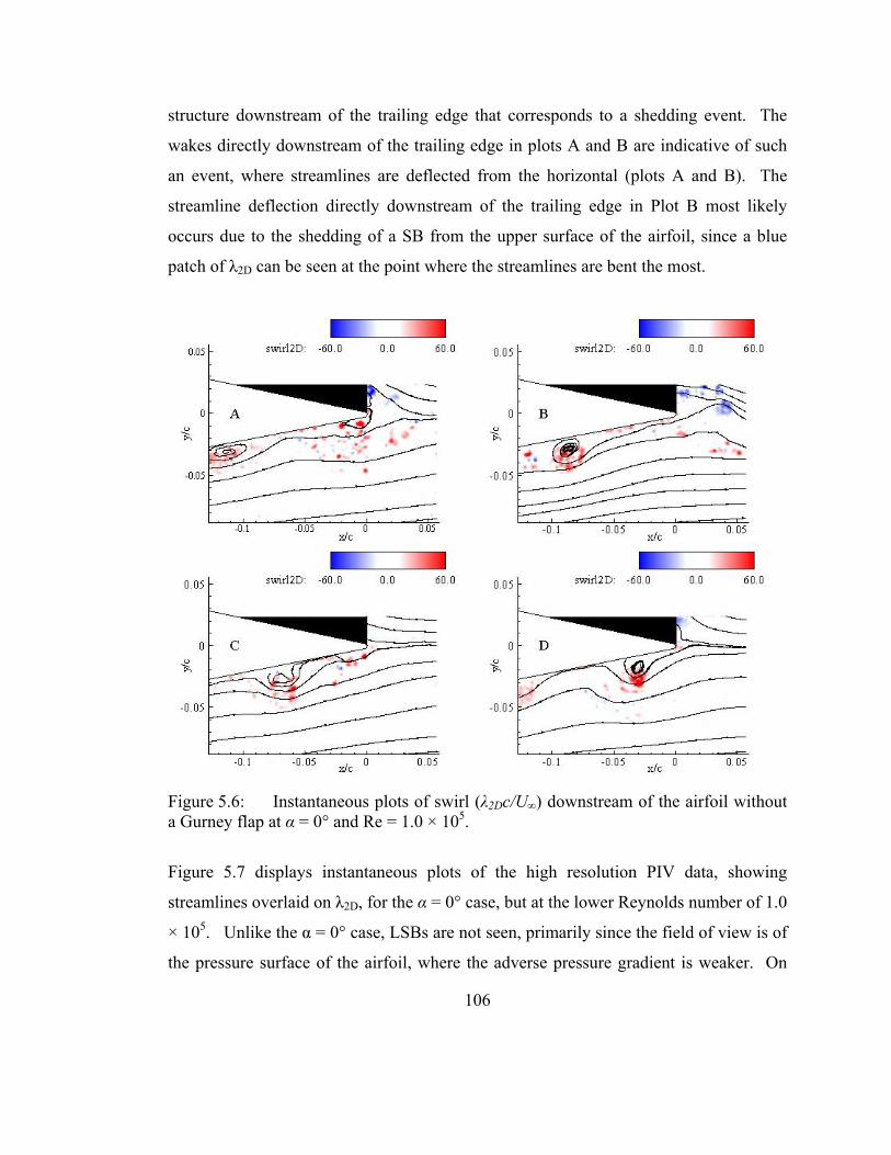
structure downstream of the trailing edge that corresponds to a shedding event. The
wakes directly downstream of the trailing edge in plots A and B are indicative of such
an event, where streamlines are deflected from the horizontal (plots A and B). The
streamline deflection directly downstream of the trailing edge in Plot B most likely
occurs due to the shedding of a SB from the upper surface of the airfoil, since a blue
patch of λ2D can be seen at the point where the streamlines are bent the most.
Figure 5.6: Instantaneous plots of swirl (λ2Dc/U∞) downstream of the airfoil without a Gurney flap at α = 0° and Re = 1.0 × 10⁵.
Figure 5.7 displays instantaneous plots of the high resolution PIV data, showing
streamlines overlaid on λ2D, for the α = 0° case, but at the lower Reynolds number of 1.0
× 105. Unlike the α = 0° case, LSBs are not seen, primarily since the field of view is of
the pressure surface of the airfoil, where the adverse pressure gradient is weaker. On
106

the upper surface of the airfoil, LSBs undoubtedly exist, as can be seen from the
numerous blue patches downstream of the trailing edge, but above the airfoil chordline
(see in particular plots A, C, and D). In addition, the streamline curvature in plots A, B,
and C indicate that LSBs are being shed into the wake, causing these disturbances.
Figure 5.7: Instantaneous plots of swirl (λ2Dc/U∞) downstream of the airfoil without a Gurney flap at α = 8° and Re = 1.0 × 10⁵.
In both the low and high Reynolds number cases at α = 8°, it can be seen that the
streamlines downstream of the airfoil are in general deflected downward much more
significantly than for the α = 0° case. This is associated with an increase in the
circulation around the airfoil and indicates an increase in lift that was seen in Chapter 3
as the angle of attack of the airfoil is increased.
107

108
5.2 Instantaneous PIV Measurements – 4% Gurney Flap
Figs. 5.8 through 5.10 show a sequence of velocity fields for the airfoil with the 4%
Gurney flap at Re = 2.1 × 10⁵ at α = 0°. Normal velocity is shown in Fig. 5.8. The
plots indicate strong oscillations in magnitude consistent with the presence of a vortex
street. Note the zone of negative normal velocity (blue) next to and directly
downstream of a zone of positive normal velocity (red) in the first two plots. This
juxtaposition corresponds directly with a compact zone of strong negative vorticity
(blue in Fig. 5.9) that traverses across the field. A juxtaposition of opposite sense (red
downstream of blue) is associated with positive vorticity (red in Fig. 5.9) that also
traverses the field (most evident in frames 3 and 4). One final point is that the normal
velocity magnitude immediately below the flap tip varies significantly indicating
intermittent shedding of fluid from the separated zone upstream of the flap.
Fig. 5.9 shows the vorticity for this sequence. The plots reveal strips of spanwise
vorticity (ω) with negative and positive sign that are shed from the upper airfoil surface
and Gurney flap tip, respectively. The clockwise vorticity (blue) shed from the upper
surface remains focused in the form of a strip that is pulled downward into the flap
wake. The positive vorticity shed from the flap tip is spread initially over a larger length
scale across the wake and shows greater intermittency in the streamwise direction.
Downstream of the trailing edge, the wake develops into an asymmetric Kármán vortex
street pattern. The areas of negative vorticity appear more focused than the areas of
positive vorticity. The wake also exhibits a net downward flow direction which is
expected given the positive lift coefficient for this configuration. The wake asymmetry
can be explained partially by the differences in flow direction at the airfoil trailing edge
and the flap tip as observed in the average fields from chapter 4 (Figs. 4.4 and 4.5).
In Fig. 5.10, the sequence with λ2D is shown. Starting with the top plot, a negative
vortex core is seen separating from the upper surface, and continuing downstream and
slightly downward until it reaches the edge of the field of view in the fourth plot.

Figure 5.8: Normal velocity (v/U∞) downstream of the airfoil with a 4% Gurney flap at α = 0° and Re = 2.1 × 10⁵.
109
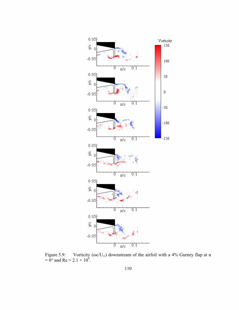
Figure 5.9: Vorticity (ωc/U∞) downstream of the airfoil with a 4% Gurney flap at α = 0° and Re = 2.1 × 10⁵.
110
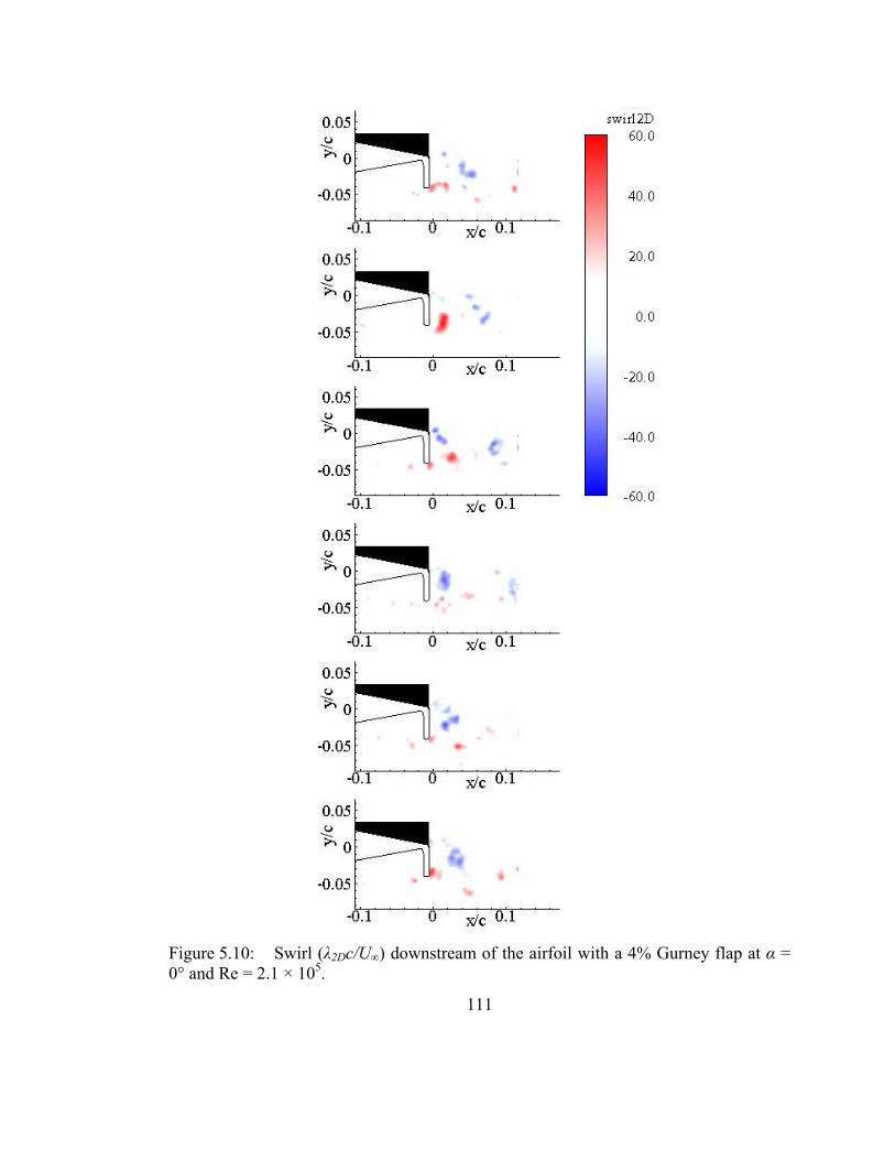
Figure 5.10: Swirl (λ2Dc/U∞) downstream of the airfoil with a 4% Gurney flap at α = 0° and Re = 2.1 × 10⁵.
111
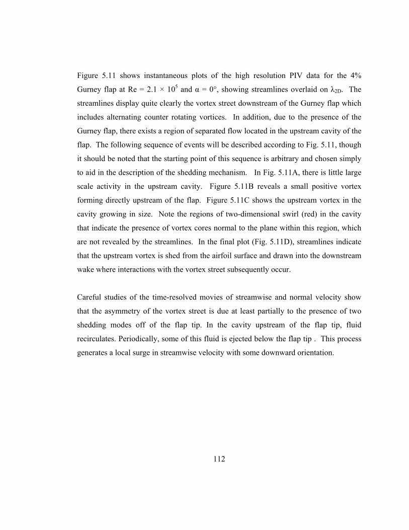
112
Figure 5.11 shows instantaneous plots of the high resolution PIV data for the 4%
Gurney flap at Re = 2.1 × 10⁵ and α = 0°, showing streamlines overlaid on λ2D. The
streamlines display quite clearly the vortex street downstream of the Gurney flap which
includes alternating counter rotating vortices. In addition, due to the presence of the
Gurney flap, there exists a region of separated flow located in the upstream cavity of the
flap. The following sequence of events will be described according to Fig. 5.11, though
it should be noted that the starting point of this sequence is arbitrary and chosen simply
to aid in the description of the shedding mechanism. In Fig. 5.11A, there is little large
scale activity in the upstream cavity. Figure 5.11B reveals a small positive vortex
forming directly upstream of the flap. Figure 5.11C shows the upstream vortex in the
cavity growing in size. Note the regions of two-dimensional swirl (red) in the cavity
that indicate the presence of vortex cores normal to the plane within this region, which
are not revealed by the streamlines. In the final plot (Fig. 5.11D), streamlines indicate
that the upstream vortex is shed from the airfoil surface and drawn into the downstream
wake where interactions with the vortex street subsequently occur.
Careful studies of the time-resolved movies of streamwise and normal velocity show
that the asymmetry of the vortex street is due at least partially to the presence of two
shedding modes off of the flap tip. In the cavity upstream of the flap tip, fluid
recirculates. Periodically, some of this fluid is ejected below the flap tip . This process
generates a local surge in streamwise velocity with some downward orientation.
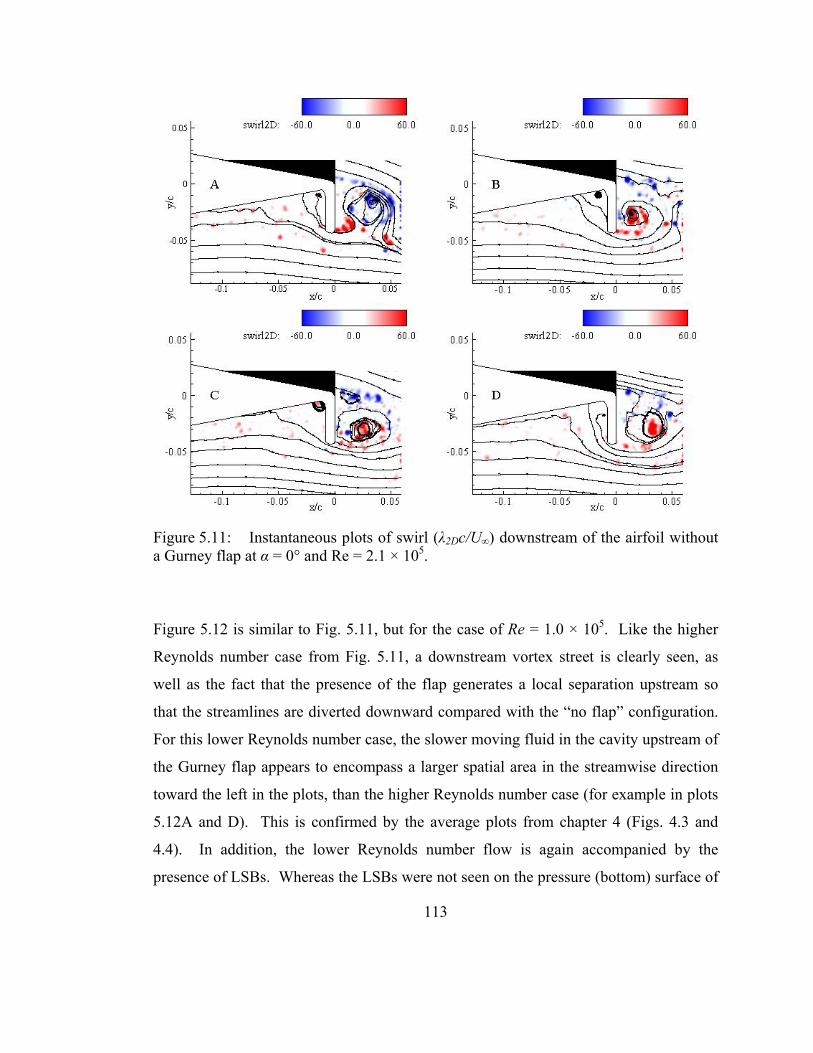
Figure 5.11: Instantaneous plots of swirl (λ2Dc/U∞) downstream of the airfoil without a Gurney flap at α = 0° and Re = 2.1 × 10⁵.
Figure 5.12 is similar to Fig. 5.11, but for the case of Re = 1.0 × 10⁵. Like the higher
Reynolds number case from Fig. 5.11, a downstream vortex street is clearly seen, as
well as the fact that the presence of the flap generates a local separation upstream so
that the streamlines are diverted downward compared with the “no flap” configuration.
For this lower Reynolds number case, the slower moving fluid in the cavity upstream of
the Gurney flap appears to encompass a larger spatial area in the streamwise direction
toward the left in the plots, than the higher Reynolds number case (for example in plots
5.12A and D). This is confirmed by the average plots from chapter 4 (Figs. 4.3 and
4.4). In addition, the lower Reynolds number flow is again accompanied by the
presence of LSBs. Whereas the LSBs were not seen on the pressure (bottom) surface of
113

the airfoil for the no-flap case, with the Gurney flap in place, the LSBs are seen on the
pressure surface. A LSB is particularly visible in Fig. 5.12C, at a location of (x/c,y/c) =
(-0.1,-0.04), as well as in Fig. 5.12D in a similar location. In the final plot, Fig. 5.12D,
the region of recirculating fluid upstream of the Gurney flap is at least partially shed
into the downstream wake, as indicated by the streamlines and the red vortex cores seen
just below the tip of the Gurney flap and continuing downstream that have a distinct
downward trajectory as indicated by the direction of the local streamlines, as compared
to the other plots, where the streamlines extending from the flap tip have only a slight
downward trajectory.
Figure 5.12: Instantaneous plots of swirl (λ2Dc/U∞) downstream of the airfoil without a Gurney flap at α = 0° and Re = 1.0 × 10⁵.
114

115
Figs. 5.13 through 5.15 are similar to Figs. 5.8 through 5.10, but showing two
sequences of velocity fields at α = 8°. The two columns represent sequences in which
the fluid from the cavity upstream of the flap is expunged into the downstream wake.
This phenomenon is characterized by a burst of negative normal velocity (seen in blue)
in the region just below the flap tip. The sequence on the left begins with a small region
of negative normal velocity just upstream of the flap tip (x/c = -0.06). As it progresses
around the flap tip in the second, third, and fourth frames, the region of positive normal
velocity (red) just downstream of the flap tip has begun to move downstream in the
wake, so that it no longer occupies the region directly downstream of the flap. The
negative burst (blue) from the upstream cavity then moves to the position downstream
of the flap that was originally occupied by the positive normal velocity in the first and
second frames. It then progresses downstream in the remaining two frames following
the patch of positive normal velocity. In this case, a fairly smooth transition occurs
from the upstream cavity to the downstream wake. The interaction between the two
shedding modes (the Kármán vortex street downstream of the flap, and the secondary
shedding mode resulting from fluid filling up the upstream cavity and then being
expunged) is seamless and smooth, since the burst of downward normal velocity from
the upstream cavity coincides with the downward normal velocity phase of the
downstream shedding. Constructive interference takes place between the two shedding
modes.
Contrast these events with those seen in the sequence on the right, in which the fluid
begins to enter the wake while the downstream shedding is forming and releasing a
region of positive normal velocity. Once again, the sequence begins with a patch of
negative normal velocity (blue) forming directly upstream of the flap tip. Directly
downstream, a region of positive normal velocity (red) is just beginning to form. The
upstream downward motion continues over the next three frames, and does not begin to
enter the downstream wake until the fifth frame. When it finally emerges and enters the

116
downstream wake, the wake is characterized by smaller regions of upward and
downward velocity, whose length scale is smaller (on the order of 1/3 to 1/2) than the
length scale seen in the first sequence. The wake is much less organized, suggesting
that the downward motion from the upstream cavity served to diminish the strength of
the upflow immediately downstream of the flap. In this case, destructive interference
occurs between the two shedding modes.
In general, the burst of negative normal velocity coming from the upstream cavity either
serves to enhance the same-signed velocity in the downstream wake, or diminish the
strength of the opposite-signed region of normal velocity. Both possibilities cause an
instantaneous increase in the circulation around the airfoil that would not exist without
the presence of the upstream shedding.
Figure 5.14 shows the normalized vorticity for the same sequence of velocity fields as
Fig. 5.13. Note in particular the region of positive vorticity (red) upstream of the
Gurney flap tip in the first plot in the left sequence. This vortex transitions to directly
beneath the flap tip in the second frame, then merges with the positive (red) vorticity
forming downstream of the flap in the third and fourth frames. The last two frames are
characterized by alternating evenly-spaced regions of positive and negative vorticity in
a clear vortex street pattern. In contrast, in the right-hand plot, smaller zones are spread
out in two rows, one above with negative vorticity, and the other below with positive
vorticity, which is more characteristic of two opposite-signed shear layers.
The difference between constructive and destructive upstream shedding is made clearer
in Fig. 5.15, where plots of signed λ2D are shown. In the constructive interference case
on the left, the positive (red) swirl is first seen upstream of the flap in the first two
frames. The third and fourth frames show the vortex core emerging from the flap tip
into the downstream vortex street. And the last two frames show very even positive and
negative vortex cores shedding into the downstream wake with a slightly downward

117
trajectory. The sequence on the right begins in a similar fashion concerning the
upstream cavity. A positive vortex core approaches the flap tip in the first frame.
However, instead of a positive vortex core forming downstream of the flap at this time,
there is a negative (blue) core in formation. The positive (red) core does not easily
merge with a vortex of opposite sign, so the last four frames show a more sporadic
separation and positioning of vortex cores.

Figure 5.13: Normal velocity (v/U∞) downstream of the airfoil with a 4% Gurney flap at α = 8° and Re = 2.1 × 10⁵. Sequence on the left shows constructive upstream shedding. Sequence on the right shows destructive upstream shedding.
118

Figure 5.14: Vorticity (ωc/U∞) downstream of the airfoil with a 4% Gurney flap at α = 8° and Re = 2.1 × 10⁵. Sequence on the left shows constructive upstream shedding. Sequence on the right shows destructive upstream shedding.
119

Figure 5.15: Swirl (λ2Dc/U∞) downstream of the airfoil with a 4% Gurney flap at α = 8° and Re = 2.1 × 10⁵. Sequence on the left shows constructive upstream shedding. Sequence on the right shows destructive upstream shedding.
120

121
Figures 5.16 and 5.17 display instantaneous plots of high resolution PIV measurements
for the 4% Gurney flap at low (1.0 × 10⁵) and high (2.1 × 10⁵) Reynolds numbers,
respectively. Plots are of streamlines overlaid on signed swirl.
At the higher Reynolds number (Fig. 5.16), the downstream vortex street is quite
visible. Variations in the spatial length of the recirculation zone in the upstream cavity
are characterized by many smaller patches of localized swirl, indicating the presence of
many positive cores of vorticity that are wrapping up due to the shear layer in this
region. A primary difference in this α = 8° case as compared to the α = 0° case (Fig.
5.11), is that due to the inclination angle of the Gurney flap, recirculating fluid in the
upstream cavity is more contained and less likely to be drawn into the downstream
wake easily. Therefore, the upstream shedding events become more coherent and
distinct. This can be seen from the intensity of vortex cores in the upstream cavity for
the α = 8° case (Fig. 5.16), where the cores are much stronger as compared to the α = 0°
case (Fig. 5.11).
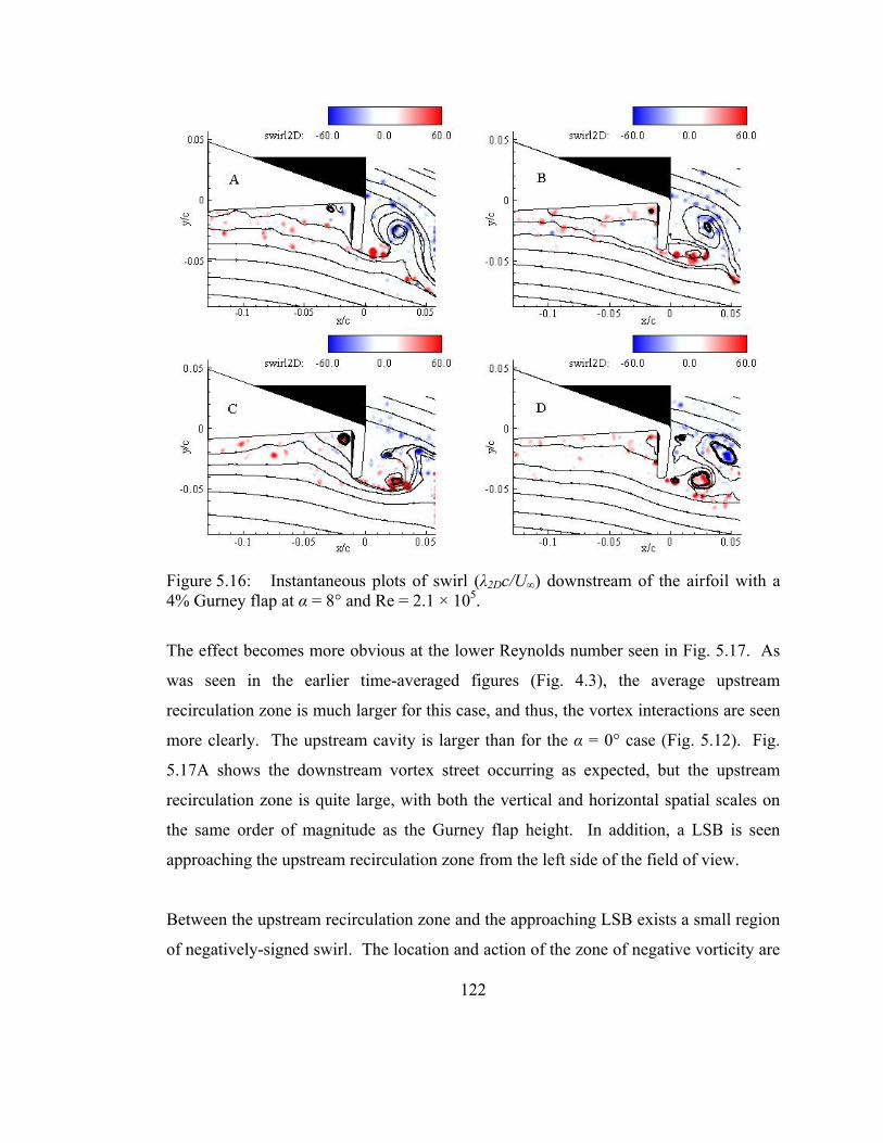
Figure 5.16: Instantaneous plots of swirl (λ2Dc/U∞) downstream of the airfoil with a 4% Gurney flap at α = 8° and Re = 2.1 × 10⁵.
The effect becomes more obvious at the lower Reynolds number seen in Fig. 5.17. As
was seen in the earlier time-averaged figures (Fig. 4.3), the average upstream
recirculation zone is much larger for this case, and thus, the vortex interactions are seen
more clearly. The upstream cavity is larger than for the α = 0° case (Fig. 5.12). Fig.
5.17A shows the downstream vortex street occurring as expected, but the upstream
recirculation zone is quite large, with both the vertical and horizontal spatial scales on
the same order of magnitude as the Gurney flap height. In addition, a LSB is seen
approaching the upstream recirculation zone from the left side of the field of view.
Between the upstream recirculation zone and the approaching LSB exists a small region
of negatively-signed swirl. The location and action of the zone of negative vorticity are
122

123
key identifiers in determining the timing of an upstream shedding event. As the
downstream portion of the larger positive vortex impinges on the upstream face of the
flap, it becomes trapped, in the sense that the flap prohibits its convection downstream
(Fig. 5.17B). Vortices further upstream continue to convect toward the trapped vortex,
compressing it spatially. Since the circulation encompassing this vortex remains nearly
constant, the rotational velocity increases. At a critical point, the rotational velocity of
the trapped vortex is sufficient to generate a local separation, dragging the recirculation
zone out into the freestream. This can be seen clearly in Fig. 5.17C where the small
blue vortex core is now located at the crux of the upstream cavity. The local shear layer
peels away from the airfoil surface and this blue vortex is dragged into the area near the
freestream, where it is quickly propelled downstream, which serves to then drag the
large trapped positive vortex out of the upstream cavity, which can be seen as the patch
of red directly below and to the left of the Gurney flap in Fig. 5.17C. With this the
spatially significant “ejection” occurs, which is the most obvious part of the upstream
shedding observed previously in the time-resolved PIV fields (Figs. 5.13 through 5.15).
The ejected structures subsequently interact with the asymmetric Kármán vortex street
that exists in the downstream wake, and the progression repeats, as Fig. 5.17D shows a
smaller upstream recirculation zone with a LSB approaching from the left. If the
ejection coincides with a similar-signed normal (downward) velocity surge in the vortex
street, the structures interfere with each other positively, creating an even larger
downward surge. Conversely, if the ejection occurs during a momentary upsurge in the
downstream vortex street, the two events interfere negatively, potentially “canceling
each other out.” Since the two shedding modes are not closely coupled, any manner of
downstream interaction between these two extremes can occur.

Figure 5.17: Instantaneous plots of swirl (λ2Dc/U∞) downstream of the airfoil with a 4% Gurney flap at α = 8° and Re = 1.0 × 10⁵.
Fig. 5.18 displays a schematic of the two modes of vortex shedding seen in the data
from the previous figures. PIV sequences and wake visualization show that the flap
acts as a forward facing step which traps fluid in the form of a weak and generally
disorganized positive vortex (shown in green). The fluid cannot escape above through
the airfoil, or downstream due to the flap. Neither can the slow moving fluid escape
downward as this would require it to cross the fast-moving, nearly streamwise velocity
present below the airfoil but outside of the boundary layer.
While slow-moving boundary layer fluid from beneath the airfoil is accumulating in the
cavity upstream of the Gurney flap, the airfoil and flap support a shape resembling an
asymmetric solid body with a blunt trailing edge. After some amount of time, the fluid
124

125
that has been accumulating in the upstream cavity has grown spatially, both downward
toward the flap tip and also upstream in the direction of the leading edge, to the point
where its normal length scale is near that of the Gurney flap height. When this occurs,
the trapped vortex achieves enough energy to penetrate or push downward the layer of
high streamwise velocity just below the Gurney flap. This is manifested in a burst of
velocity downward, as the recirculating fluid escapes the cavity, and an accompanying
burst in streamwise velocity.
This downward velocity component induces a similar downward component of velocity
on the fluid and vortex structures directly downstream of the Gurney flap. During this
instant, the flow downstream of the flap attains a relatively large component of negative
normal velocity that momentarily increases the circulation on the airfoil, thus increasing
the lift. This also helps to explain the shape and deflection of the time-averaged velocity
magnitude plots. A histogram of the normal velocity measured at the tip of the 4%
Gurney flap at α = 0° and Re = 2.1 × 10⁵ can be seen in Fig. 5.19; its bimodal
distribution indicates normal velocity in primarily two modes, when the upstream
vortex is weak but gaining strength, and when the vortex is expunged from the cavity.

Figure 5.18: Schematic of the bimodal vortex shedding occurring at the trailing edge of the airfoil with a Gurney flap. Positive vorticity is indicated in red; negative vorticity is indicated in blue. The green areas represent fluid “trapped” in the upstream cavity. Arrows represent general trajectories of flow structures. Figure reproduced from Troolin et al. (2006).
Figure 5.19: Normalized normal velocity PDF at the point below the 4% Gurney flap tip at α = 0° and Re = 2.1 × 10⁵. Figure reproduced from Troolin et al. (2006).
126

127
5.3 Instantaneous PIV Measurements – 4% Gurney Flap Filled In
Time resolved sequences of the flow downstream of the airfoil with a filled in flap are
now considered in order to gain insight into the affect of the upstream cavity on the
flow in the downstream wake.
Figs. 5.20 through 5.22 show sequences of velocity fields for the airfoil with the 4%
filled-in Gurney flap at Re = 2.1 × 10⁵. Sequences on the left are at α = 0°, and
sequences on the right are at α = 8°.
Normal velocity is shown in Fig. 5.20. The left sequence (α = 0°) shows characteristics
of a typical vortex street downstream of an object with a blunt trailing edge, with
strong, evenly spaced regions of normal velocity forming immediately downstream of
the trailing edge. The right sequence (α = 8°) contains a region of general disorder
occurring directly downstream of the flap which is characterized by low magnitude, but
primarily upward velocity. Coherent patches of significant positive and negative
normal velocity do not manifest themselves until greater than 0.05c downstream of the
flap, and are further characterized by much smaller regions of positive and negative
normal velocity on the order of half the size of similar regions in the α = 0° case,
indicating that the vortex shedding is occurring at a higher frequency as the angle of
attack is increased. The central portion of the wake has weaker negative or downward
velocity zones (blue) than the 4% open flap case (Fig. 5.13), consistent with the
diminished lift value for this case (However, the reduced downward velocities in the
lower portion of the wake are likely a stronger factor). This was also seen in the time-
averaged plots in Fig. 4.6, where the angle of the streamlines did not show significant
downward deflection.
The point downstream of the trailing edge where the shear layers from the top and
bottom portions of the airfoil begin to interact is seen more clearly in Fig. 5.21, where

128
normalized vorticity is plotted for the two angles of attack. At α = 0° (left sequence),
the shear layers cross the centerline of the trailing edge at a streamwise location
immediately downstream, whereas for the α = 8° case (right), the shear layers do not
begin to interact until farther downstream near x/c = 0.06 and beyond.
The swirl plots in Fig. 5.22 further confirm the characteristics of the vortex shedding for
the two angles of attack. The left sequence (α = 0°) has larger, regularly-spaced vortex
cores of alternating sign being shed into the downstream wake. Examining the fourth
frame on the left side, vortex cores of positive sign are spaced by approximately x/c =
0.08 in the streamwise direction. The right sequence (α = 8°) has smaller vortex cores
that form further downstream and close examination of the fourth frame on the right
side indicates vortex cores of positive sign are spaced approximately x/c = 0.04 in the
streamwise direction.
Airfoils with the filled in Gurney flap exhibit many characteristics of vortex shedding
downstream of an object with a blunt trailing edge. No evidence of upstream vortex
shedding was observed due to the non-existence of an upstream cavity from which
recirculating fluid could be shed.
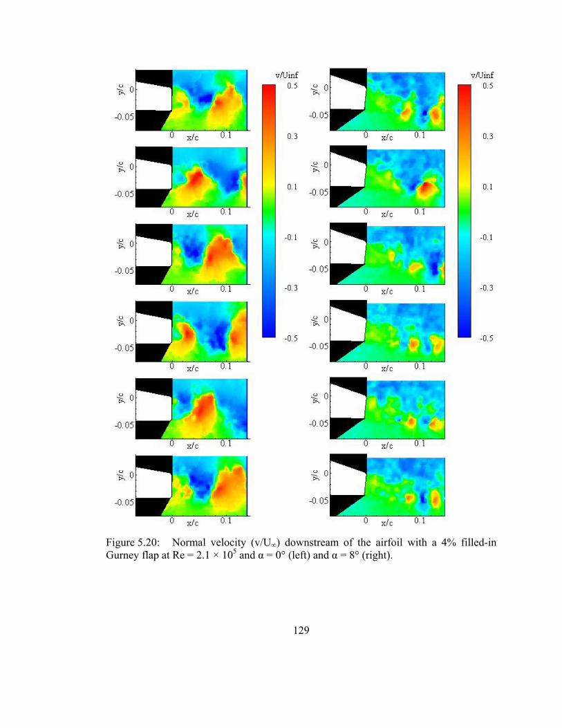
Figure 5.20: Normal velocity (v/U∞) downstream of the airfoil with a 4% filled-in Gurney flap at Re = 2.1 × 10⁵ and α = 0° (left) and α = 8° (right).
129

Figure 5.21: Vorticity (ωc/U∞) downstream of the airfoil with a 4% filled-in Gurney flap at Re = 2.1 × 10⁵ and α = 0° (left) and α = 8° (right).
130

Figure 5.22: Swirl (λ2Dc/U∞) downstream of the airfoil with a 4% filled-in Gurney flap at Re = 2.1 × 10⁵ and α = 0° (left) and α = 8° (right).
131

132
Chapter 6
6 Results and Discussion: Frequency
Measurements
This chapter discusses frequency measurements downstream of the airfoils. Hotfilm
anemometry was used to measure the velocity fluctuations downstream of airfoils with
and without Gurney flaps. The hotfilm measurements were analyzed by obtaining the
power spectra of each configuration at angles of attack ranging from α = 0° to α = 12°.
Spectra are plotted on a log-log scale, and the values for the various angles of attack
have been shifted on the vertical axis by 103 in order to better differentiate data from
each angle. The results and the relationship with the previously discussed time-resolved
velocity data are discussed in this chapter.
Unless otherwise specified, the measurements were taken at a distance of 0.7c
downstream of the trailing edge at the same y-position as the Gurney flap tip (or at the
same height as the trailing edge for the no-flap case). The measurement duration was
104 seconds at a sampling rate of 20 kHz and filtered at 10 kHz to prevent aliasing.
6.1 Frequency Data – No Gurney Flap
The airfoil without the Gurney flap displayed spectra with few or no large dominant
peaks. Plots of the power spectra for the airfoil without a Gurney flap at four angles of
attack and Reynolds number of 2.1 × 10⁵ are shown in Fig. 6.1. The α = 0° case shows
several very small peaks near 450 Hz and 600 Hz. These small peaks contain relatively
little energy and are likely due to the small amount of vortex shedding seen in the time-
resolved velocity fields from the finite thickness of the airfoil trailing edge.

Figure 6.2 shows the spectra for the airfoil without a Gurney flap at the lower Reynolds
number of 1.0 × 10⁵. The plots at lower angles of attack show more distinct peaks than
for the higher Reynolds number case, and these are likely due to the periodic shedding
of LSBs as were seen in the high resolution PIV data from chapter 5. These peaks for
the α = 0° case are located at 124 Hz, 156 Hz, 188 Hz, 219 Hz, and 283 Hz. At α = 4°,
the peaks appear to shift to slightly higher frequencies of 150 Hz, 175 Hz, 203 Hz, and
230 Hz.
For both Reynolds numbers, no dominant frequencies are seen at the higher angles of
attack of α = 8° and α = 12°, which is consistent with the PIV results, where no LSBs
were observed at α = 8° (Figs. 5.5 and 5.7).
Figure 6.1: Frequency spectra for α = 0°, 4°, 8°, and 12° for the airfoil without a Gurney flap at Re = 2.1 × 10⁵.
133

Figure 6.2: Frequency spectra for α = 0°, 4°, 8°, and 12° for the airfoil without a Gurney flap at Re = 1.0 × 10⁵.
6.2 Frequency Data – 4% Gurney Flap
Power spectra for the airfoil with a 4% Gurney flap at Re = 2.1 × 10⁵ are shown in Fig.
6.3. For the α = 0° case, one dominant peak is seen at 371 Hz, which corresponds to a
Strouhal number (St = hf/U∞) based on the freestream velocity and the height of the
trailing edge with Gurney flap of St = 0.186. Also visible in the plot is a very small
magnitude harmonic (at twice the frequency) to the right of the dominant peak. The
dominant frequency peak is due to the presence of vortices being shed downstream of
the Gurney flap. As α increases from 0° to 12°, the Strouhal number decreases
approximately linearly from 0.186 to 0.164. Frequency spectra plotted for other airfoil
shapes with Gurney flaps have resulted in similar trends and magnitudes for the
Strouhal number (see Jeffrey et al. 2000). This decreasing trend is due to the nature of
vortex shedding, where the shedding frequency decreases as the distance between upper 134

and lower shear layers increases. As α increases, the boundary layer thickness on the
suction surface increases, thereby increasing this distance, and lowering the shedding
frequency (Blake 1986).
Figure 6.3: Frequency spectra for α = 0°, 4°, 8°, and 12° for the airfoil with a 4% Gurney flap at Re = 2.1 × 10⁵. This trend can also be explained by the idea that the cross-sectional length scale
perpendicular to the free stream increases with increasing angle of attack. The absolute
shedding frequency must then decrease to maintain a constant Strouhal number based
on this scale.
135
Of interest in this study is the secondary peak at a slightly lower frequency that begins
to form and increase in magnitude as the angle of attack increases. It is most easily seen
as the hump located just to the left of the highest peak in the α = 8° case, and as the
dominant peak in the α = 12° case, that has increased in magnitude so that it is larger
than the peak due to the downstream vortex shedding. The frequency ratio between the

136
first and second shedding modes for α = 12° and 8°, are 0.74 and 0.77 respectively.
This second lower frequency that emerges as the angle of attack increases represents the
fluid shedding from the upstream cavity. Previous observations of time-resolved PIV
sequences (Figs. 5.13 through 5.15) indicate that the frequency at which the trapped
fluid is expunged from the upstream cavity is somewhat lower than that of the Kármán
shedding frequency. (The existence of this weaker peak was not mentioned by Jeffrey
et al., 2000). The spectral plots suggest that at low angles of attack, the recirculation
zone upstream of the flap is shedding fluid in a manner that does not exhibit a strongly
periodic event. At higher angles of attack, however, the upstream cavity forms a niche
that more easily blocks fluid from passing into the downstream wake. For this reason, a
more structured event is required to expunge the build-up of slower-moving fluid. This
is manifested in a more periodic form of upstream shedding.
Figure 6.4 displays the locations where additional hot-film spectral measurements were
taken for the case of the airfoil at α = 8° with the 4% Gurney flap. Also shown are the
resulting Strouhal numbers based on the freestream velocity (U∞), Gurney flap height
(h), and the frequency peaks seen in the spectra. The dominant frequency in the
upstream region of the cavity corresponded with St = 0.126. Downstream of the cavity,
this peak was also apparent in addition to the stronger peak corresponding with the
Kármán shedding frequency, St = 0.163. This pattern of peak frequencies further
suggests that there exists in the cavity upstream of the flap a mode of fluid shedding
which is distinct from the Kármán shedding that dominates the downstream wake. In
addition, the upstream and downstream shedding are coupled, in that both types affect
the vortex formation and interaction downstream. The TRPIV visualization showed that
the upstream activity has a significant effect on the downstream wake of the airfoil;
namely, contributing a net downward velocity to the wake. The coupled shedding
behavior described here was also observed at α = 0° though in a much less periodic
manner. Hot-film measurements for the airfoil with no Gurney flap revealed no

equivalent spectral peaks. Further, the peak at St = 0.126 was not observed at locations
further than one-third chord length upstream of the 4% flap.
Figure 6.4: Peak Strouhal numbers (St = fh/U∞) observed from hot-film spectra at various locations on an airfoil with a 4% Gurney flap at α = 8° and Re = 2.1 × 10⁵.
Figure 6.5 is similar to Fig. 6.3, but for lower Reynolds number (1.0 × 10⁵). In the α =
0° and α = 8° cases, two frequency peaks are present, corresponding to the two modes
of shedding. The primary peaks occur at St = 0.186 and 0.179, and the secondary peaks
occur at St = 0.163 and 0.150 for the α = 0° and 8° cases, respectively. The ratio of
secondary to primary frequencies is 0.88 for α = 8°, and 0.84 for α = 0°. The α = 4°
case appears to have only one very small frequency peak (St = 0.152) which seems to
correspond to the upstream shedding when compared with the other angles of attack.
At all angles where a peak is present, the lower frequency peak representing the
upstream shedding is larger and more distinct. As was seen in the high resolution PIV
measurements, this is due to the fact that large LSBs form along the pressure surface of
the airfoil, interact with the upstream cavity, and are subsequently shed into the
downstream wake. At α = 12°, no dominant peaks are visible. At this Reynolds
number, 12° is very close to the stall angle (approximately 13°) of the airfoil, so
separation on the suction surface is likely causing a turbulent wake without dominant
shedding patterns.
137

Figure 6.5: Frequency spectra for α = 0°, 4°, 8°, and 12° for the airfoil with a 4% Gurney flap at Re = 1.0 × 10⁵.
6.3 Frequency Data – 4% Gurney Flap Filled In
Spectral plots for the case of the 4% filled-in flap at Re = 2.1 × 10⁵ are plotted in Fig.
6.6 for comparison. Similar to the 4% open flap (Fig. 6.3), the α = 0° case shows only
one dominant peak with a corresponding harmonic at twice its value. The Strouhal
number associated with this frequency is 0.200. At α = 4°, the Strouhal number dips
slightly to 0.193, before increasing to 0.222 and 0.247 for the α = 8° and α = 12° cases,
respectively. All of the angles plotted exhibit a harmonic value at exactly twice the
peak frequency. No secondary lower frequency peaks are seen in these plots as
compared to the open flap case. Notice the distinct shift in the single dominant peak to
a higher shedding frequency as compared to the open flap case (Fig. 6.3). Even at α =
0°, the dominant peak for the closed flap is 400 Hz, and the dominant peak for the open
flap is 371 Hz. The closed flap configuration has a much more regular form of 138
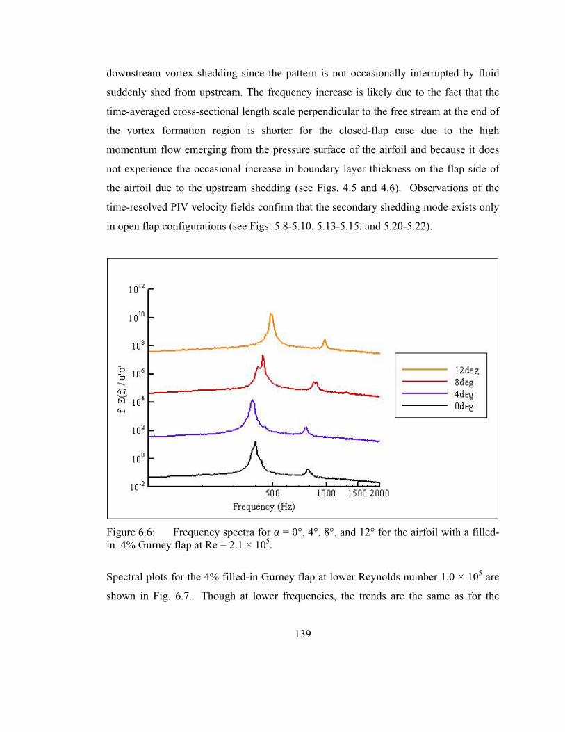
downstream vortex shedding since the pattern is not occasionally interrupted by fluid
suddenly shed from upstream. The frequency increase is likely due to the fact that the
time-averaged cross-sectional length scale perpendicular to the free stream at the end of
the vortex formation region is shorter for the closed-flap case due to the high
momentum flow emerging from the pressure surface of the airfoil and because it does
not experience the occasional increase in boundary layer thickness on the flap side of
the airfoil due to the upstream shedding (see Figs. 4.5 and 4.6). Observations of the
time-resolved PIV velocity fields confirm that the secondary shedding mode exists only
in open flap configurations (see Figs. 5.8-5.10, 5.13-5.15, and 5.20-5.22).
Figure 6.6: Frequency spectra for α = 0°, 4°, 8°, and 12° for the airfoil with a filled-in 4% Gurney flap at Re = 2.1 × 10⁵.
Spectral plots for the 4% filled-in Gurney flap at lower Reynolds number 1.0 × 10⁵ are
shown in Fig. 6.7. Though at lower frequencies, the trends are the same as for the
139

higher Reynolds number, namely, there exists one dominant frequency peak
corresponding to the vortex shedding occurring in the downstream vortex street.
Figure 6.7: Frequency spectra for α = 0°, 4°, 8°, and 12° for the airfoil with a filled-in 4% Gurney flap at Re = 1.0 × 10⁵.
Additional frequency plots for the case of the 2% Gurney flap can be seen in Appendix
C. In general, the trends are the same for the 2% flap case as for the 4% flap case. The
one exception is the 2% flap case at the lower Reynolds number of 1.0 × 10⁵, in which
the shedding frequency increases with increased angle of attack for both the open and
filled case. In addition, this case did not contain a secondary shedding frequency peak
corresponding to the upstream shedding. The reason for this is that as the Reynolds
number decreases, the boundary layers on the airfoil become thicker, and laminar
separation bubbles form upstream of the flap. The large separated region upstream of
the 1% and 2% Gurney flaps at low Reynolds number (see Figs. B1 and B3) becomes
trapped in the upstream cavity and does not shed into the downstream wake. The airfoil
then exhibits shedding characteristics similar to a filled airfoil. 140

141
6.4 Summary
Tables 6.1 and 6.2 provide a summary of the primary and secondary shedding
frequencies and Strouhal numbers for the 2% and 4% Gurney flaps at Re = 2.1 × 10⁵
and Re = 1.0 × 10⁵, respectively. Blank entries indicate that no frequency was observed
for that configuration.
Re = 2.1 × 10⁵
Alpha Primary Secondary Primary Secondary Ratio of
Gurney Flap (deg)
Frequency
(Hz)
Frequency
(Hz) St# (1) St# (2)
St#(2 )/
St#(1)
4% 0 371 0.186
4 337 0.170
8 323 250 0.163 0.126 0.77
12 323 239 0.164 0.121 0.74
2% 0 626 0.168
4 560 400 0.151 0.108 0.71
8 475 326 0.128 0.088 0.69
12 418 318 0.113 0.086 0.76
4% Filled 0 400 0.200
4 384 0.193
8 440 0.222
12 488 0.247
2% Filled 0 584 0.156
4 589 0.159
8 659 0.178
12 769 0.208
Table 6.1: Summary of the primary and secondary shedding frequency for the 2% and 4% Gurney flaps at Re = 2.1 × 10⁵.

142
Re = 1.0 × 10⁵
Alpha Primary Secondary Primary Secondary Ratio of
Gurney Flap (deg)
Frequency
(Hz)
Frequency
(Hz) St# (1) St# (2)
St#(2)/
St#(1)
4% 0 176 154 0.186 0.163 0.88
4 142 0.152
8 166 139 0.179 0.150 0.84
12
2% 0 154 0.087
4 200 0.115
8 262 0.151
12
4% Filled 0 181 0.192
4 207 0.222
8 227 0.244
12
2% Filled 0 220 0.125
4
8
12
Table 6.2: Summary of the primary and secondary shedding frequency for the 2% and 4% Gurney flaps at Re = 1.0 × 10⁵.
Figure 6.8 shows a graph of the Strouhal number versus angle of attack for the 2%, 4%,
open, and filled-in flap configurations at Re = 2.1 × 10⁵. The trend becomes quite clear
in that the shedding frequency for the open flap configurations decreases as the angle of
attack increases, while the shedding frequency for the filled-in flap configurations
increases as the angle of attack increases. In addition, data points corresponding with
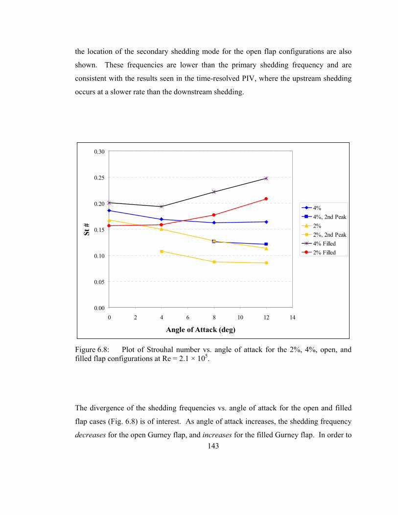
the location of the secondary shedding mode for the open flap configurations are also
shown. These frequencies are lower than the primary shedding frequency and are
consistent with the results seen in the time-resolved PIV, where the upstream shedding
occurs at a slower rate than the downstream shedding.
0.00
0.05
0.10
0.15
0.20
0.25
0.30
0 2 4 6 8 10 12 14
Angle of Attack (deg)
St #
4%4%, 2nd Peak2%2%, 2nd Peak4% Filled2% Filled
Figure 6.8: Plot of Strouhal number vs. angle of attack for the 2%, 4%, open, and filled flap configurations at Re = 2.1 × 10⁵.
The divergence of the shedding frequencies vs. angle of attack for the open and filled
flap cases (Fig. 6.8) is of interest. As angle of attack increases, the shedding frequency
decreases for the open Gurney flap, and increases for the filled Gurney flap. In order to 143

144
understand this relationship, it is necessary to again examine the streamlines of the
time-averaged velocity fields. Figures 4.5 and 4.6 show the time-averaged streamwise
velocity for the open and filled flaps at α = 0° and 8° and Re = 2.1 × 10⁵. Note the
location of the end of the vortex formation region, indicated by the point where the
streamlines from the upper and lower surfaces close up downstream of the trailing edge.
This represents the streamwise length of the downstream wake. For the 4% open case
(Fig. 4.5), the length is approximately 0.045c for both α = 0° and 8° cases. The length
for the 4% filled case at α = 0° (Fig. 4.6 top) is similar at approximately 0.042c.
However, for the 4% filled case (Fig. 4.6 bottom), the downstream wake is much longer
at approximately 0.07c. The length of the vortex formation region is important because
is dictates the point at which the vortices roll up and shed from the body (Griffin 1995).
Figure 6.9 shows individual instantaneous vorticity plots for the 4% open flap at α = 0°
and 8° and the 4% filled flap at α = 0° and 8°, taken from previous Figs. 5.9, 5.14, and
5.21. Note that the vortex formation occurs directly downstream of the trailing edge
(within about 0.02c) for the open cases (top left and right) and for the filled α = 0°
(bottom left) case. However, for the α = 8° case (bottom right), the shear layers extend
downstream and do not rollup into separate vortex structures until approximately 0.06c
downstream, when the distance between shear layers has narrowed. Since the effective
distance between shear layers becomes shorter for the filled case as the angle of attack
increases, the vortex shedding increases.

Figure 6.9: Instantaneous plots of vorticity (ωc/U∞) downstream of an airfoil with a 4% Gurney flap at α = 0° (top left) and α = 8° (top right), and with a 4% filled Gurney flap at α = 0° (bottom left) and α = 8° (bottom right) at Re = 2.1 × 10⁵.
145

146
Chapter 7
7 Conclusions
7.1 Force Measurements and Flow Visualization
Results of force balance measurements and flow visualization were presented. The
quantitative measurements of the absolute lift coefficient, as well as qualitative
visualizations provide a good basis for the understanding of the effects of the Gurney
flap on an airfoil at low Reynolds number. Key conclusions from this data are as
follows:
• The presence of a Gurney flap on an airfoil at low Reynolds number served to
increase the lift generated on the body. As the height of the Gurney flap was
increased, the lift also increased. For the 1%, 2%, and 4% Gurney flaps, the lift
coefficient was increased by an average of 0.09, 0.21, and 0.36, respectively.
The slope of the lift curve did not change noticeably with the presence of a
Gurney flap.
• An airfoil with a 4% Gurney flap was compared against an airfoil with a 4%
Gurney flap where the upstream cavity of the flap was “filled-in” along a
straight line between the tip of the flap and a point ⅓-chord upstream of the
trailing edge. The effect was a decrease in the generated lift for the filled-in
case (increase in lift coefficient over the no-flap configuration of only an
average of 0.16), suggesting that a significant portion of the increased lift
increment produced by the Gurney flap results directly from flow phenomena
occurring in the upstream cavity, and its influence on the trailing wake.
147
• Flow visualization did not reveal a significant difference in stall angle of attack
for the airfoil with and without the Gurney flap.
• Flow visualization revealed that as the angle of attack is increased, the
separation region upstream of the Gurney flap on the pressure side of the airfoil
also increased in size (in the streamwise direction, progressing from the flap
upstream).
7.2 Time-Averaged
Ensemble averaged PIV measurements were used to examine the nature of the flow
around an airfoil with a Gurney flap. Specifically, averaged velocity fields from high
resolution PIV at the leading and trailing edge of an airfoil without a Gurney flap and
airfoils with 1%, 2%, and 4% Gurney flaps were examined at Reynolds numbers of 1.0
× 105 and 2.1 × 10⁵. Several key conclusions can be drawn from this data:
• For the airfoil without a Gurney flap, the average velocity plots revealed
evidence of a laminar separation bubble (LSB) seen forming in the area of
adverse pressure gradient of the airfoil at both α = 0° and α = 8°, on the pressure
surface, at the lower Reynolds number. For the α = 8° case, the LSB appears to
be convecting downstream. At the higher Reynolds number, no evidence of
LSBs was seen for the current measurement locations.
• For airfoils with Gurney flaps, a pair of counter-rotating vortices are seen
downstream of the flap.
• At α = 0°, the streamlines downstream of the airfoils with Gurney flaps were
deflected downward as compared to the airfoil without, which had streamlines
that maintained a horizontal trajectory downstream of the trailing edge.

148
• For the airfoil with the 4% Gurney flap, the boundary layer on the suction (top)
surface of the airfoil was significantly thinner at the higher Reynolds number of
2.1 × 10⁵ as compared to the Re = 1.0 × 10⁵ case.
• For airfoils with Gurney flaps, there exists an area of decreased streamwise
velocity directly upstream of the flap that increases in length as the angle of
attack is increased from 0° to 8° (which is consistent with the tuft
visualizations), and decreases in length as the Reynolds number is increased.
• The zone of recirculating fluid downstream of the flap decreases in streamwise
length as the angle of attack is increased for Re = 1.0 × 10⁵, but increases in
length for Re = 2.1 × 10⁵ which is directly related to the upstream recirculation
zone.
• The airfoil with a 4% filled-in Gurney flap revealed less downward deflection of
the downstream streamlines than the open case.
• The 4% filled-in flap also revealed a suction surface boundary layer thickness
that was approximately twice as thick as for the 4% open flap.
• The presence of a Gurney flap has the effect of shifting the leading edge
stagnation point on the airfoil toward the pressure surface of the airfoil, which is
associated with increased circulation, and thus lift, which is consistent with the
force measurements.

149
7.3 Time-Resolved
Time-resolved velocity information was presented to gain understanding into the
evolution of flow patterns and the nature of the fluid mechanical structures in the area
around the trailing edge of an airfoil with a Gurney flap. While it is somewhat intuitive
that the Gurney flap increases lift by adding to the effective camber of the wing, the
less-obvious advantage of the Gurney flap lies in the complex flow structure
surrounding it. TRPIV is an effective tool in studying this structure due to the presence
of recirculation, unsteadiness, and coherent vortices that form at more than one
frequency. TRPIV provides a field-based temporal history that can capture the
dynamics of the flow. The Gurney design, which includes both a blunt trailing edge and
a single-sided leading edge, generates both a “standard” wake of alternating counter-
rotating vortices with fairly predictable frequency and the additional single-signed
vortices shed from the cavity upstream of the flap tip at a lower frequency. The flow
sequences reveal that the intermittent release of fluid from the cavity induces a net
negative normal velocity on the airfoil wake increasing the circulation, and thus the lift.
This phenomenon served to increase the lift at every angle of attack measured. The
TRPIV velocity fields revealed the nature of the upstream and downstream shedding
modes, their interactions, and their dependence upon the flap height. Key conclusions
for the TRPIV data are as follows:
• The velocity field sequences generated by the TRPIV method revealed a mode
of vortex shedding not previously observed or postulated in experimental or
numerical investigations of flow around Gurney flaps. A loosely organized
vortex forms and grows in the cavity upstream of the flap until it is expunged
into the airfoil wake where it interacts with the Kármán vortex street that forms
directly downstream of the flap. The two shedding modes are of different
frequency and interact downstream of the flap to generate constructive or
destructive interference depending on the phases during which they merge. In

150
all cases, these interactions served to increase the negative normal velocity in
the airfoil wake, and thus the circulation and lift, as compared to the closed flap
case.
• The upstream vortex shedding was not present in a case with a “filled-in” flap
that generated approximately half the lift increment of the open-cavity case.
Thus, it appears that a significant part of the lift increment produced by the
Gurney flap results directly from the upstream shedding and its influence on the
trailing wake.
• Although the lift increment for a given flap length is fairly constant for different
angles of attack, examination of TRPIV sequences and spectra suggests that the
coherence of the shedding of upstream fluid increases and the related shedding
frequency decreases with increasing angle of attack.
• Also, since the volume of “trapped” fluid is expected to decrease with
decreasing flap length, it is expected that the corresponding shedding frequency
would increase.
7.4 Frequency
Spectra from hot-film measurements revealed the nature of the upstream and
downstream shedding modes, their interactions, and their dependence upon the flap
height. The key conclusions are:
• Two shedding modes of different frequency interact downstream of the flap to
generate constructive or destructive interference depending on the phases during
which they merge. In all cases, these interactions served to increase the negative

151
normal velocity in the airfoil wake, and thus the circulation and lift, as compared
to the closed flap case.
• The different flap heights displayed very similar wake and shedding interference
patterns at the higher Reynolds number of 2.1 × 10⁵, with the coherent structures
in each scaling approximately with the height of the flap. For example, Strouhal
numbers associated with the primary and secondary shedding modes at α = 8°
were (0.163, 0.126) and (0.128, 0.088) for the 4% and 2% flaps respectively.
• The ratio of primary to secondary shedding modes was found to be similar for
the two flap heights of 4% and 2% at 0.77 and 0.69 respectively, suggesting that
the shedding mode ratio is independent of the Gurney flap height, as long as
coherent shedding modes exist.
• The Strouhal number decreases as angle of attack increases for the airfoil with a
flap at Re = 2.1 × 10⁵. This is due to the thickening boundary layer on the
suction (upper) surface which increases the distance between the shear layers
and decreases the shedding frequency.
• The Strouhal number increases as angle of attack increases for the airfoil with
the fill-in Gurney flap at Re = 2.1 × 10⁵. This is due to the extended vortex
formation region downstream of the blunt trailing edge. The upper and lower
shear layers do not roll up into separate vortex structures until further
downstream where the wake width has narrowed and the distance between shear
layers has decreased, which increases the shedding frequency.
• At the lower Reynolds number of 1.0 × 10⁵, the 4% Gurney flap showed similar
characteristics as at the higher Reynolds number, with decreasing shedding
frequency with increasing angle of attack; however, the 2% Gurney flap did not

152
show this trend, and showed an increase in shedding frequency with increasing
angle of attack. It also did not contain a secondary shedding frequency peak
corresponding to the upstream shedding. As the Reynolds number decreases,
the boundary layers on the airfoil become thicker. The large separated region
upstream of the 1% and 2% Gurney flaps at low Reynolds number (see Figs B1
and B3) becomes trapped in the upstream cavity and does not shed into the
downstream wake, so that the airfoil exhibits shedding characteristics similar to
a filled airfoil.
7.5 Summary and Recommendations for Future Work
The purpose of this study was to examine the nature of the flow around an airfoil with a
Gurney flap at low Reynolds numbers. The following is a brief summary of the
findings, as well as some unanswered questions and possibilities for future work in this
area. In addition, some possible improvements to the investigation techniques used in
this study are addressed.
Force and moment measurements, hot-film anemometry, high resolution PIV, and time-
resolved PIV experiments were performed successfully to determine the lift, spectra,
and 2D velocity fields in the region around symmetric airfoils with Gurney flaps. The
measurements were used to compute the vortex shedding frequency and the 2D vorticity
fields in the region of the Gurney flap.
What is the overall effect of a Gurney flap on airfoil performance?
The presence of a Gurney flap on an airfoil has the effect of increasing the lift while
increasing the drag only minimally for flaps with length scales approximately equal to
or less than the local boundary layer thickness at the trailing edge. Due to the flap, the

153
effective camber of the airfoil is increased; the forward stagnation point of the airfoil
shifts towards the pressure surface.
What is the nature of the flow structures in the region of the Gurney flap?
Periodic shedding of counter-rotating vortices is found downstream of the Gurney flap.
The frequency of the vortex shedding decreases with increased flap height and
increased angle of attack. The cavity upstream of the Gurney flap also plays an
important role in the downstream wake, as slower moving fluid in the form of a laminar
separation bubble becomes trapped upstream of the GF, then grows in size until it is
expunged into the wake, interacting with the regular vortex pattern downstream and
creating a net negative normal velocity that increases the circulation. An airfoil with
the upstream cavity filled in produced approximately half of the increase in lift. The
angle of attack of the airfoil has a significant effect on the shedding upstream of the
flap, with higher angles of attack producing more periodic upstream shedding. At low
Reynolds numbers and with short Gurney flaps (in this case, Re = 1.0 × 10⁵ and 2%
flap), the recirculation zone upstream of the flap does not shed in a periodic way, so that
the airfoil exhibits shedding characteristics similar to that of an airfoil with a filled in
flap.
Though the current study was fairly comprehensive, many aspects of Gurney flap
performance remain to be examined. This study used only two Reynolds numbers that
were within the same order of magnitude. As has been seen in the literature, airfoil
characteristics are highly dependent on Reynolds number especially within the lower
range of this study. Further research would be required to understand the effects of the
Gurney flap as the Reynolds number is both increased and decreased further.
Decreased Reynolds numbers would cast light on the area of micro air vehicles and the
nature of seemingly unstable insect flight. Higher Reynolds numbers would provide
information on the potential benefit to larger transport and military aircraft, where the

154
high lift of a Gurney flap may offer significant benefits in allowing high-speed aircraft
to land at slower speeds, thereby increasing safety and decreasing tire and brake wear.
A research aspect that would provide significant amounts of insight would be an
experimental setup that allowed high resolution and time resolved data to be captured
simultaneously around the entire airfoil. At the time of this study, such technologies are
prohibitively expensive, but with time will become available.

155
Bibliography Adrian R (1997) “Dynamic ranges of velocity and spatial resolution of particle image velocimetry,” Meas. Sci. Technol. 8, pp 1393-8. Adrian R; Christensen K; Liu Z (2000), “Analysis and interpretation of instantaneous turbulent velocity fields.” Exp. Fluids 29, pp. 275-290. Bechert D W, Meyer R, Hage W (2000) “Drag Reduction of Airfoils with Miniflaps. Can we Learn from Dragonflies?” AIAA, Fluids 2000, Denver, CO, June 19-22. Blake W (1986), “Mechanics of Flow-Induced Sound and Vibration” Vol. II, Academic Press, Inc., pp. 756-782. Buchholz M D, Tso J (2000) Lift Augmentation on Delta Wing with Leading-Edge Fences and Gurney Flap, Journal of Aircraft, Vol. 37, No. 6, pp 1050-1057. Burgmann S, Brucker C, Schroder W (2006) Scanning PIV measurements of a laminar separation bubble. Exp. in Fluids 41, pp. 319–326. Byerley A R, Störmer O, Baughn J W, Simon T W, Treuren K W, List J (2003) “Using Gurney Flaps to Control Laminar Separation on Linear Cascade Blades,” ASME, Vol. 125, pp. 114-120. Carrannanto P G, Storms B L, Ross J C, CummingsR M (1998) “Navier-Stokes analysis of lift-enhancing tabs on multi-element airfoils” Aircraft Design pp 145-158. Feller, Myere (1976) Development of a controllable particle generator for LV seeding in hypersonic wind tunnels, Minnesota Symposium on Laser Anemometry, Bloomington, Minn., October 22-24, 1975, Proceedings. (A77-44283 20-35) Minneapolis, University of Minnesota, 1976, p. 343-357. Finn J E (2005) “How to measure turbulence with hot-wire anemometers – A practical guide,” Dantec Dynamics. Skovlunde, Denmark. Gai S L, Palfrey R (2003) Influence of Trailing-Edge Flow Control on Airfoil Performance, Journal of Aircraft. 40(2) pp. 332-7. Gerontakos P, Lee T (2006) “Oscillating Wing Loadings with Trailing-Edge Strips,” Journal of Aircraft. 47(2) pp. 428-36.

156
Giguere P, Dumas G, Lemay J (1997) “Gurney Flap Scaling for Optimum Lift-to-Drag Ratio.” AIAA Journal, 35(12) pp.1888-90. Glauert H (1923) The Interference of Wind Channel Walls on the Aerodynamic Characteristics of Airfoil. Reports and Memoranda No. 867, March, 1923. British Aeronautical Research Committee. Glauert H (1926) The Elements of Airfoil and Airscrew Theory. Chap. XI. Cambridge University Press, 1926. Griffin O M (1995) A note on bluff body vortex formation. Journal of Fluid Mechanics 284, pp. 217-24. Guzel G, Sankar S, Rhee M (2005) Computational Investigation of the Effects of Gurney Flap on the Aerodynamic Performance of VR-12 Airfoil, AIAA 2005-4960, 23rd AIAA Applied Aerodynamics Conference, Toronto, Ontario, Canada, 6 – 9 June. Hain R, Kahler C, Radespiel R (2009) “Dynamics of laminar separation bubbles at low-Reynolds-number aerofoils,” J. Fluid Mech. Vol. 630, pp. 129-153. Horton H P (1968) Laminar separation bubbles in two-and three- dimensional incompressible flow. Ph.D. thesis, University of London. “Hot Film and Hot wire Anemometry: Theory and Application,” (1978) Technical Bulletin TB5, Thermo-Systems Inc., St. Paul, MN. “IFA 300 Constant Temperature Anemometer System,” (2007) Operation Manual, TSI Inc., St. Paul, MN. Jacobs E N, Anderson R F (1930) Large-Scale Aerodynamic Characteristics of Airfoils as tested in the Variable Density Tunnel. N. A. C. A. Technical Report No. 352, 1930. Jacobs E N, Sherman A (1937), “Airfoil section characteristics as affected by variations of the Reynolds number,” NACA Langley Memorial Aeronautical Laboratory (Langley Field, VA, United States) NACA Report 586, pp. 41. Jang C; Ross J; Cummings R (1998), “Numerical investigation of an airfoil with a Gurney flap.” Aircraft Design 1, pp. 75-88. Jeffrey D; Zhang X; Hurst D (2000), “Aerodynamics of Gurney Flaps on a Single-Element High-Lift Wing,” Journal of Aircraft, Vol. 37. No. 2, pp. 295-301.

157
Keane R; Adrian R (1990) “Optimization of Particle Image Velocimeters. Part 1: Double Pulsed Systems,” Meas. Sci. Tech. 1, pp. 1202-15. Keane R D; Adrian R J (1991) “Optimization of Particle Image Velocimeters: II. Multiple Pulsed Systems,” Meas. Sci. Tech. 2, pp. 963-74. Kinzel M. P., Maughmer M. D., Lesieutre G. L. (2005) Numerical Investigation on Miniature Trailing-Edge Effectors on Static and Oscillating Airfoils, AIAA 2005-1039, 43rd AIAA Aerospace Sciences Meeting and Exhibit, Reno, Nevada, 10-13 January. Ladson C L; Brooks C W; Hill A S (1996) Computer Program To Obtain Ordinates for NACA Airfoils, NASA TM 4741. Lee H T, Kroo I M (2004) “Computational Investigation of Airfoils with Miniature Trailing Edge Control Surfaces,” AIAA, 2004-1051. Lee L, Lee T (2007) “Effect of Gurney Flap on Unsteady Wake Vortex.” Journal of Aircraft, 44(4), pp. 1398-1401. Lee T; Birch D; Gerontakos P (2004) “Testing Unmanned Aerial Vehicle Airfoils,“ IEEE Instrumentation and Measurement Magazine, 7(3), pp. 32-7. Li Y. C., Wang J. J. (2003) “Experimental Studies on the Drag Reduction and Lift Enhancement of a Delta Wing,” Journal of Aircraft, 40(2), pp. 277–281. Li Y, Wang J, Zhang P (2002) Effects of Gurney Flaps on a NACA 0012 Airfoil. Flow, Turbulence and Combustion, 68: 27-39, 2002. Liebeck R (1978), “Design of subsonic airfoils for high lift.” Journal of Aircraft 15(9), pp. 547-61. Lin J C, Pauley L L (1996) “Low-Reynolds-Number Separation on an Airfoil,“ AIAA Journal 34(8), pp 1570-7. Lin J L, Wei C Y, Lin, C Y (2007) “Aerodynamic performance of thin wings at low Reynolds numbers.” Aircraft Engineering and Aerospace Technology: An International Journal, 73(9), pp 245-53. Liu T, Montefort J (2007) “Thin-Airfoil Theoretical Interpretation for Gurney Flap Lift Enhancement.” Journal of Aircraft, 44(2), pp. 667-671. Liu T, Montefort J , Liou W, Pantula S R, Shams Q A (2007) “Lift Enhancement by Static Extended TE.” Journal of Aircraft, 44(6), pp. 1939 -1947.

158
Lorkowski T, Hermle F, Fervel M, Sagansan A (2004) “Distributed Electromechanical Actuation for Adaptive Flight Control Elements,” Recent Advances in Aerospace Actuation Systems and Components, November 24-26, 2004, Toulouse, France. Matalanis C G, Eaton J K (2006) Wake Vortex Control Using Rapidly Actuated Segmented Gurney Flaps, AIAA 2006-481, 44th AIAA Aerospace Sciences Meeting and Exhibit, Reno, Nevada, 9-12 January 2006. Matalanis C G, Eaton J K (2007) “Wake Vortex Control Using Static Segmented Gurney Flaps.” AIAA Journal 45(2), pp. 321-328. Matalanis C G (2007) “Wake Vortex Alleviation Using Rapidly Actuated Segmented Gurney Flaps.” Ph.D. Thesis. Stanford University. Meyer R, Hage W, Bechert D W, Schatz M, Thiele F (2006) “Drag Reduction on Gurney Flaps by 3D Modifications.” Journal of Aircraft 43(1), pp. 132-140. Moyse R, Lietsche J-C, Scholz D, Zingel H, Hayashibara S, Heron I (2006) Flow Visualization Study on the Effect of a Gurney Flap in a Low Reynolds Number Compressor Cascade, AIAA 2006-7809, 6th AIAA Aviation Technology, Integration and Operations Conference, Wichita, Kansas, 25-27 September. Munk M M (1923) The Determination of the Angles of Attack of Zero Lift and Zero Moment, Based on Munk’s Integrals. N. A. C. A. Technical Note No. 122, 1923. Munk M M (1925) Elements of the Wing Section Theory and of the Wing Theory. N. A. C. A. Technical Report No. 191, 1925. Munk, Max M., and Miller, Elton W. (1925) The Variable Density Wind Tunnel of the National Advisory Committee for Aeronautics. N. A. C. A. Technical Report No. 227, 1925. Myose R, Heron I, Papdakis M (1996) “Effect of Gurney flaps on a NACA 0011 Airfoil.” AIAA, Aerospace Sciences Meeting and Exhibit, 34th, Reno, NV, Jan. 15-18, 1996. Myose R, Papadakis M, Heron I (1998) “Gurney Flap Experiments on Airfoils, Wings, and Reflection Plane Model.” Journal of Aircraft 35(2). Neuhart D; Pendergraft O (1988), “A water tunnel study of Gurney flaps.” NASA TM 4071.
159
Nikolic V R (2006a) “Trailing Vortex Rollup from a Wing Equipped with a Gurney Flap.” Journal of Aircraft 43(2). Nikolic V R (2006b) “Effect of Full Span Gurney Flap Height on Wing Wake Vortex Alleviation.” Journal of Aircraft 45(2). Nikolic V R (2006c) “Additional Aerodynamic Features of Wing Gurney Flap Flows.” Journal of Aircraft 45(2). O’Meara M, Mueller T (1987) “Laminar separation bubble characteristics on an airfoil at low Reynolds numbers,” AIAA Journal 25(8):1033-1041. Papadakis M, Myose R, Matallana S (1997) “Experimental investigation of Gurney flaps on a two element general aviation airfoil” AIAA, Aerospace Sciences Meeting & Exhibit, 35th, Reno, NV, Jan. 6-9, 1997. Prandtl, L (1921) Application of Modern Hydrodynamics to Aeronautics. Part II, section F. N. A. C. A. Technical Report No. 116. Price, J (2001) “Unsteady Measurements and Computations on an Oscillating Airfoil with Gurney Flaps.” M.S. Thesis. North Carolina State University. Rhee, M (2004) A Computational Study of an Oscillating VR-12 Airfoil with a Gurney Flap, AIAA 2004-5202, 22nd Applied Aerodynamics Conference and Exhibit, Providence Rhode Island, 16-19 August. Shyy W, Klevebring F, Nilsson M, Sloan J, Carroll B, Fuentes C (1999) “Rigid and Flexible Low Reynolds Number Airfoils.” Journal of Aircraft, 36(3), pp. 523-9. Singh M K, Dhanalakashmi K, Chakrabartty S K (2007) “Navier-Stokes Analysis of Airfoils with Gurney Flap.” Journal of Aircraft, 44(5), pp. 1487-93. Solovitz S (2002) “Experimental Aerodynamics of Mesoscale Trailing Edge Actuators.” Ph.D. Thesis. Stanford University. Solovitz S, Eaton J (2002) “Experimental Aerodynamics of Mesoscale Trailing-Edge Actuators,” AIAA Journal, 40(12), pp. 2538-2540. Solovitz S, Eaton J (2004a), “Spanwise Response Variation for Partial-Span Gurney-Type Flaps,” AIAA Journal, 42(8), pp. 1640-1643.

160
Solovitz S, Eaton J (2004b) “Dynamic Flow Response Due to Motion of Partial-Span Gurney-Type Flaps,” AIAA Journal, 42(9), pp. 1729-1736. Storms B L, Jang C S (1994) “Lift Enhancement of an Airfoil Using a Gurney Flap and Vortex Generators,” Journal of Aircraft, 31(3), p. 542. Tang D, Dowell E H (2007) “Aerodynamic Loading for an Airfoil with an Oscillating Gurney Flap.” Journal of Aircraft, 44(4), pp. 1245-1257. Thomas P J, Butefisch K A (1993) An investigation of the influence of the size distribution of seeding particles on LDA velocity data in the vicinity of a large velocity gradient, Phys. Fluids A, 5(11) pp. 2807-2814. Torres G E, Mueller T J (2004) “Low-Aspect-Ratio Wing Aerodynamics at Low Reynolds Numbers.” AIAA Journal, 42(5), pp865-73. Traub L W, Galls S F (1999) “Effects of Leading- and Trailing-edge Gurney Flaps on a Delta Wing.” Journal of Aircraft, 36(4), pp 651-658. Traub L W, Miller A C, Rediniotis O (2006) “Preliminary Parametric Study of Gurney Flap Dependencies.” Journal of Aircraft, 43(4), pp 1242-1244. Traub L W, Agarwal G (2007) “Exploratory Investigation of Geometry Effects on Gurney Flap Performance.” Journal of Aircraft, 44(1), pp 351-353. Troolin, D R, Longmire E K, and Lai W T (2006a) "Time-resolved PIV analysis of flow over a NACA 0015 airfoil with Gurney flap," Exp. in Fluids 41:241-254. Troolin D R, Longmire E K, Lai W T (2006b) “The Effect of Gurney Flap Height on Vortex Shedding Modes Behind Symmetric Airfoils,” 13th Int. Symp. on Applications of Laser Techniques to Fluid Mechanics, Lisbon, Portugal, 26-29 June, 2006. Troolin D R, Longmire E K (2007) “Large Format PIV to Resolve Large and Small Structures Surrounding a Gurney Flap,” 7th International Symposium on Particle Image Velocimetry, Roma, Italia, September 11-14, 2007. Viieru D, Albertani R, Shyy W, Ifju P G (2005) “Effect of Tip Vortex on Wing Aerodynamics of Micro Air Vehicles.” Journal of Aircraft 42(6), pp. 1530-6. Wadcock A (1987), “Investigations of low-speed turbulent separated flow around airfoils.” NASA CR 177450.
161
Wang J J, Li Y C, Choi K S (2008) “Gurney Flap - Lift Enhancement, Mechanisms and Applications,” Progress in Aerospace Sciences 44, pp. 22-47. Wang J J, Zhan J X, Zhang W, Wu Z (2006) “Application of a Gurney Flap on a Simplified Forward Swept Aircraft Model.” Journal of Aircraft, 43(5), pp 1561-1564. Wereley S T, Gui L (2003) “A Correlation-Based Central Difference Image Correction (CDIC) Method and Application in a Four-Roll Mill Flow PIV Measurement.” Exp. in Fluids 34:42-51. Wheeler A J, Ganji A R (1996) “Introduction to Engineering Experimentation,” Prentice-Hall, Inc. White F M (1991) "Viscous Fluid Flow," McGrawHill. Yee K, Joo W, Lee D H (2007) “Aerodynamic Performance Analysis of a Gurney Flap for Rotorcraft Application.” Journal of Aircraft, 44(3), pp. 1003-1014. Zerihan J, Zhang X (2000) “Force Enhancement of Gurney Flaps on a Wing in Ground Effect Fluids.” AIAA Fluids 2000, Denver, CO, June 19-22. Zerihan J, Zhang X (2001) “Aerodynamics of Gurney Flaps on a Wing in Ground Effect,” AIAA Journal. Vol. 39 No. 5. Zhan J X, Wang J J (2004) Experimental Study on Gurney Flap and Apex Flap on a Delta Wing, Journal of Aircraft, Vol. 41, No. 6, pp 1379-1383. Zhang W, Hain R, Kahler C (2008) “Scanning PIV investigation of the laminar separation bubble on a SD7003 airfoil,” Exp. In Fluids 45:725–743.

162
Appendix A
A Airfoil Coordinates
The following tables give the coordinates of the airfoils used in this study. The
coordinates for the airfoils were calculated according to the equations given in Ladson
et al. (1996). The origin for these sets of coordinates is at the airfoil leading edge.

163
0% Gurney x/c y/c, up y/c, low 0.0000 0.0000 0.0000 0.0167 0.0250 -0.0250 0.0333 0.0375 -0.0375 0.0527 0.0458 -0.0458 0.0667 0.0500 -0.0500 0.0833 0.0542 -0.0542 0.1000 0.0583 -0.0583 0.1217 0.0625 -0.0625 0.1333 0.0646 -0.0646 0.1500 0.0667 -0.0667 0.1667 0.0689 -0.0689 0.1833 0.0708 -0.0708 0.2000 0.0724 -0.0724 0.2167 0.0735 -0.0735 0.2333 0.0744 -0.0744 0.2500 0.0750 -0.0750 0.3000 0.0749 -0.0749 0.3500 0.0744 -0.0744 0.4000 0.0728 -0.0728 0.4500 0.0708 -0.0708 0.5000 0.0667 -0.0667 0.5500 0.0633 -0.0633 0.6000 0.0591 -0.0591 0.6500 0.0540 -0.0540 0.7000 0.0480 -0.0480 0.7500 0.0409 -0.0409 0.8000 0.0333 -0.0333 0.8500 0.0253 -0.0253 0.9000 0.0167 -0.0167 0.9500 0.0089 -0.0089 0.9667 0.0064 -0.0064 0.9833 0.0035 -0.0035 0.9917 0.0020 -0.0020 1.0000 0.0000 0.0000
Table A.1: Coordinates for the standard NACA0015 airfoil.

164
1% Gurney x/c y/c, up y/c, low 0.0000 0.0000 0.0000 0.0167 0.0250 -0.0250 0.0333 0.0375 -0.0375 0.0527 0.0458 -0.0458 0.0667 0.0500 -0.0500 0.0833 0.0542 -0.0542 0.1000 0.0583 -0.0583 0.1217 0.0625 -0.0625 0.1333 0.0646 -0.0646 0.1500 0.0667 -0.0667 0.1667 0.0689 -0.0689 0.1833 0.0708 -0.0708 0.2000 0.0724 -0.0724 0.2167 0.0735 -0.0735 0.2333 0.0744 -0.0744 0.2500 0.0750 -0.0750 0.3000 0.0749 -0.0749 0.3500 0.0744 -0.0744 0.4000 0.0728 -0.0728 0.4500 0.0708 -0.0708 0.5000 0.0667 -0.0667 0.5500 0.0633 -0.0633 0.6000 0.0591 -0.0591 0.6500 0.0540 -0.0540 0.7000 0.0480 -0.0480 0.7500 0.0409 -0.0409 0.8000 0.0333 -0.0333 0.8500 0.0253 -0.0253 0.9000 0.0167 -0.0167 0.9500 0.0089 -0.0089 0.9667 0.0064 -0.0064 0.9833 0.0035 -0.0035 0.9917 0.0020 -0.0054 0.9917 0.0020 -0.0149 1.0000 0.0000 -0.0149 1.0000 0.0000 0.0000
Table A.2: Coordinates for the NACA0015 airfoil with 1% Gurney flap.
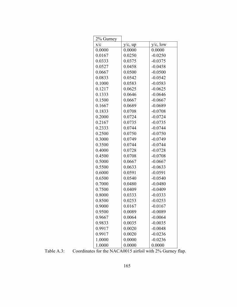
165
2% Gurney x/c y/c, up y/c, low 0.0000 0.0000 0.0000 0.0167 0.0250 -0.0250 0.0333 0.0375 -0.0375 0.0527 0.0458 -0.0458 0.0667 0.0500 -0.0500 0.0833 0.0542 -0.0542 0.1000 0.0583 -0.0583 0.1217 0.0625 -0.0625 0.1333 0.0646 -0.0646 0.1500 0.0667 -0.0667 0.1667 0.0689 -0.0689 0.1833 0.0708 -0.0708 0.2000 0.0724 -0.0724 0.2167 0.0735 -0.0735 0.2333 0.0744 -0.0744 0.2500 0.0750 -0.0750 0.3000 0.0749 -0.0749 0.3500 0.0744 -0.0744 0.4000 0.0728 -0.0728 0.4500 0.0708 -0.0708 0.5000 0.0667 -0.0667 0.5500 0.0633 -0.0633 0.6000 0.0591 -0.0591 0.6500 0.0540 -0.0540 0.7000 0.0480 -0.0480 0.7500 0.0409 -0.0409 0.8000 0.0333 -0.0333 0.8500 0.0253 -0.0253 0.9000 0.0167 -0.0167 0.9500 0.0089 -0.0089 0.9667 0.0064 -0.0064 0.9833 0.0035 -0.0035 0.9917 0.0020 -0.0048 0.9917 0.0020 -0.0236 1.0000 0.0000 -0.0236 1.0000 0.0000 0.0000
Table A.3: Coordinates for the NACA0015 airfoil with 2% Gurney flap.

166
4% Gurney x/c y/c, up y/c, low 0.0000 0.0000 0.0000 0.0167 0.0250 -0.0250 0.0333 0.0375 -0.0375 0.0527 0.0458 -0.0458 0.0667 0.0500 -0.0500 0.0833 0.0542 -0.0542 0.1000 0.0583 -0.0583 0.1217 0.0625 -0.0625 0.1333 0.0646 -0.0646 0.1500 0.0667 -0.0667 0.1667 0.0689 -0.0689 0.1833 0.0708 -0.0708 0.2000 0.0724 -0.0724 0.2167 0.0735 -0.0735 0.2333 0.0744 -0.0744 0.2500 0.0750 -0.0750 0.3000 0.0749 -0.0749 0.3500 0.0744 -0.0744 0.4000 0.0728 -0.0728 0.4500 0.0708 -0.0708 0.5000 0.0667 -0.0667 0.5500 0.0633 -0.0633 0.6000 0.0591 -0.0591 0.6500 0.0540 -0.0540 0.7000 0.0480 -0.0480 0.7500 0.0409 -0.0409 0.8000 0.0333 -0.0333 0.8500 0.0253 -0.0253 0.9000 0.0167 -0.0167 0.9500 0.0089 -0.0089 0.9667 0.0064 -0.0064 0.9833 0.0035 -0.0035 0.9917 0.0020 -0.0048 0.9917 0.0020 -0.0442 1.0000 0.0000 -0.0442 1.0000 0.0000 0.0000
Table A.4: Coordinates for the NACA0015 airfoil with 4% Gurney flap.
167
Appendix B
B Additional Average PIV Plots
Plots of the averaged velocity fields for the 1% and 2% flaps are shown. It is interesting
to note that the trends are consistent between the 4% and 2% flap cases. (The same
trends are also observable in averaged velocity fields of the 1% flap case). In contrast
to the 4% case, where the flap length is large compared to the unperturbed boundary
layer thickness, the two smaller flaps have length more comparable to the thickness, as
determined using Blake’s (1986) estimate of displacement thickness for blunt trailing
edges, and are more relevant to practical applications. As Wadcock (1987) determined
previously for higher Reynolds numbers (and therefore thinner boundary layers),
Gurney flaps did not cause appreciable increases in drag until they extended beyond
about 2% of the chord length.
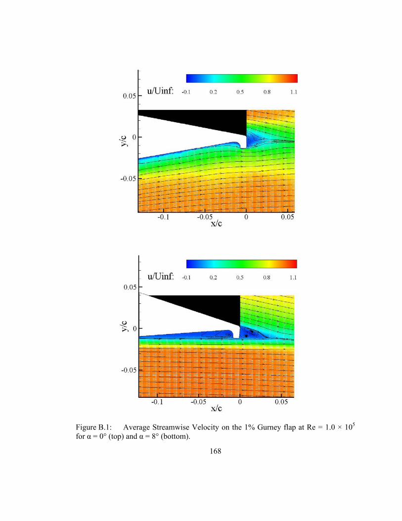
Figure B.1: Average Streamwise Velocity on the 1% Gurney flap at Re = 1.0 × 10⁵ for α = 0° (top) and α = 8° (bottom).
168

Figure B.2: Average Streamwise Velocity on the 1% Gurney flap at Re = 2.1 × 10⁵ for α = 0° (top) and α = 8° (bottom).
169

Figure B.3: Average Streamwise Velocity on the 2% Gurney flap at Re = 1.0 × 10⁵ for α = 0° (top) and α = 8° (bottom).
170

Figure B.4: Average Streamwise Velocity on the 2% Gurney flap at Re = 2.1 × 10⁵ for α = 0° (top) and α = 8° (bottom).
171

Figure B.5: Average of 50 PIV fields at the airfoil leading edge at Rec = 1.0 × 10⁵ for the 1% Gurney flap at α = 0° (top) and α = 8° (bottom). Color contours represent normalized streamwise velocity.
172

Figure B.6: Average of 50 PIV fields at the airfoil leading edge at Rec = 2.1 × 10⁵ for the 1% Gurney flap at α = 0° (top) and α = 8° (bottom). Color contours represent normalized streamwise velocity.
173

Figure B.7: Average of 50 PIV fields at the airfoil leading edge at Rec = 1.0 × 10⁵ for the 2% Gurney flap at α = 0° (top) and α = 8° (bottom). Color contours represent normalized streamwise velocity.
174

Figure B.8: Average of 50 PIV fields at the airfoil leading edge at Rec = 2.1 × 10⁵ for the 2% Gurney flap at α = 0° (top) and α = 8° (bottom). Color contours represent normalized streamwise velocity.
175

176
Appendix C
C Frequency Data for 2% Gurney Flap
Spectra for the airfoil with a shorter 2% Gurney flap at Re = 2.1 × 10⁵ are plotted in Fig.
C.1. Trends for the smaller flap height are similar to those for the larger flap. At α =
0°, there is one dominant peak at St = 0.168, with a very small harmonic to the right.
As the angle of attack increases, additional peaks emerge. At α = 4°, the dominant peak
decreases to St = 0.151, and a very small secondary peak begins to emerge slightly to
the left of the dominant peak at St = 0.108. As the angle of attack increases to α = 8°,
the primary and secondary peaks are of almost equal strength and correspond to
Strouhal numbers of St = 0.128 and 0.088, respectively. At α = 12°, the secondary peak
corresponding to upstream shedding has surpassed the primary peak in magnitude, with
additional smaller peaks appearing at surrounding frequencies, which may be due to
periodic shedding beginning to occur on the airfoil suction surface.

Figure C.1: Frequency spectra for α = 0°, 4°, 8°, and 12° for the airfoil with a 2% Gurney flap at Re = 2.1 × 10⁵.
The spectra for the 2% filled-in Gurney flap at Re = 2.1 × 10⁵ are shown in Fig. C.2.
The plots are characterized by the presence of one dominant peak and its corresponding
harmonic at twice the frequency. At α = 0°, there are several small peaks, with the
dominant peak occurring at 584 Hz (St = 0.156), as the angle of attack increases, the
frequency of the dominant peak increases, and the smaller peaks disappear.
177

Figure C.2: Frequency spectra for α = 0°, 4°, 8°, and 12° for the airfoil with a filled-in 2% Gurney flap at Re = 2.1 × 10⁵.
Figures C.3 and C.4 show the spectra for the 2% Gurney flap open and filled-in,
respectively, at Re = 1.0 × 10⁵. Interestingly, this smaller flap height at lower Reynolds
number did not show the same characteristics as the larger flap at the same Reynolds
number, or the same size flap at the higher Reynolds number. For the open case (Fig.
C.3), instead of the primary frequency peak decreasing, as in the other open-flap cases,
the primary frequency increases as the angle of attack increases (from St = 0.041 at α =
0°, to St = 0.054 at α = 4°, to St = 0.071 at α = 8°). For this case, the 2% filled-in
Gurney flap at Re = 1.0 × 10⁵, a dominant peak is only seen at α = 0° (St = 0.059), and
the other higher angles of attack do not exhibit any significant frequency peaks.
178

Figure C.3: Frequency spectra for α = 0°, 4°, 8°, and 12° for the airfoil with a 2% Gurney flap at Re = 1.0 × 10⁵.
179
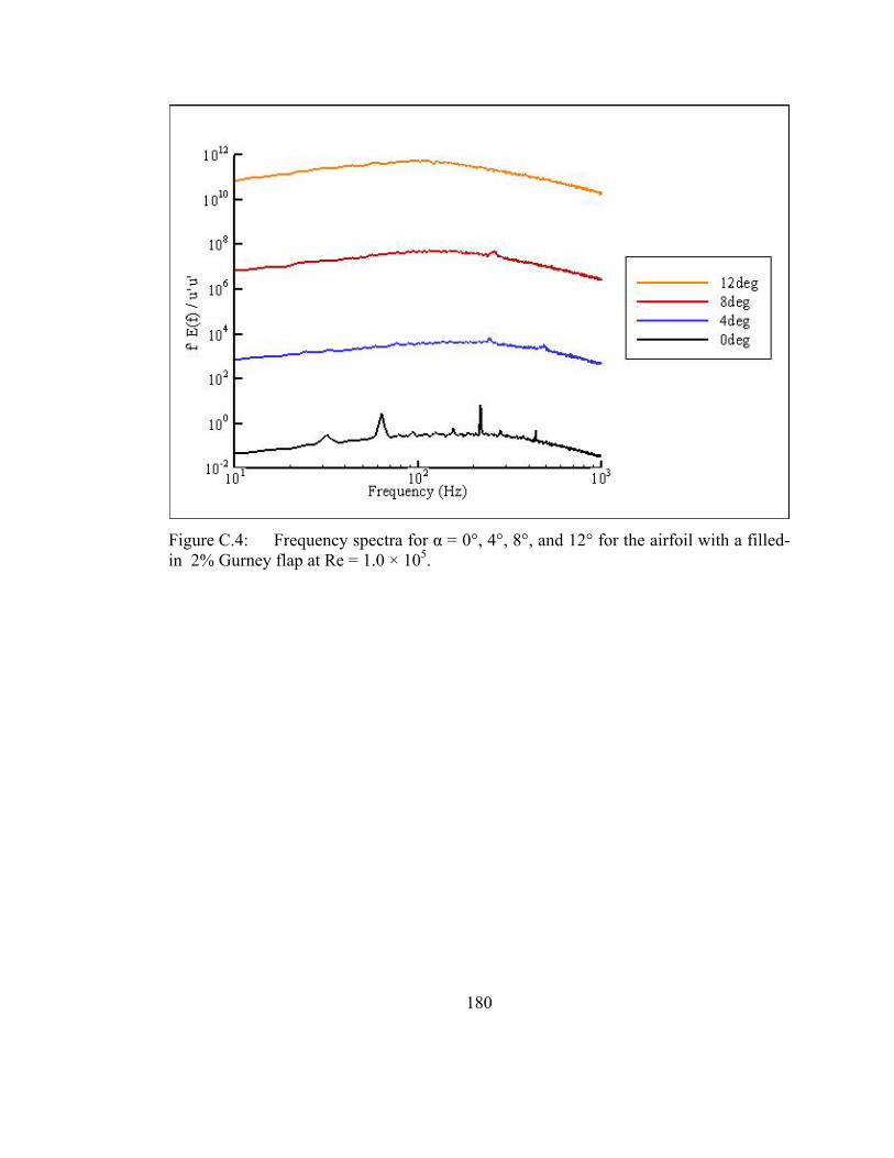
Figure C.4: Frequency spectra for α = 0°, 4°, 8°, and 12° for the airfoil with a filled-in 2% Gurney flap at Re = 1.0 × 10⁵.
180