1

A Quadruple Tank Process Control Experiment

Effendi Rusli, Siong Ang, and Richard D. Braatz

Department of Chemical and Biomolecular Engineering University of Illinois at Urbana-Champaign

600 South Mathews Avenue, Box C-3 Urbana, Illinois 61801

Keywords: Process control education, Right half plane transmission zeros, Time-varying dynamics, Multivariable control, Decoupling control

Abstract

A quadruple tank apparatus was developed for use in undergraduate chemical engineering

laboratories that illustrates the performance limitations for multivariable systems posed by ill-conditioning,

right half plane transmission zeros, and model uncertainties. The most novel aspect of the apparatus is that it

has a configuration in which the time-varying movement of a right half plane transmission zero across the

imaginary axis makes it impossible to control the process with a linear feedback controller. This appears to

be the first educational laboratory experiment designed to clearly illustrate the extreme effects that time-

varying dynamics can have on controllability of the process. Example identification and control results

illustrate the use of the experiment in an undergraduate process control laboratory.

1. Introduction

While analytical calculations and process simulations [1,2] should be a key component in the

education of a chemical engineer, students gain a deeper understanding of the nonidealities of industrial

processes by carrying out experiments. Many industrial control problems are nonlinear and have multiple

manipulated and controlled variables. It is common for models of industrial processes to have significant

uncertainties, strong interactions, and/or nonminimum phase behavior (i.e., right half plane transmission

zeros). Chemical engineering students especially find the concept of right half plane transmission zeros to be

subtler than other concepts.

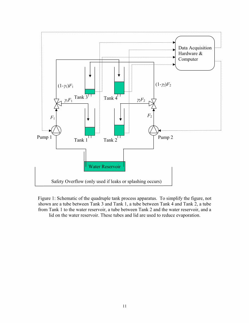
A quadruple tank process was designed and constructed to give undergraduate chemical engineers

laboratory experience with key multivariable control concepts (see Fig. 1). By changing two flow ratios in

the apparatus, a range of multivariable interactions can be investigated using only one experimental

apparatus. Since Spring 1999, this quadruple tank process has been used to teach students at the University

of Illinois in the following skills:

1. understanding control limitations due to interactions, model uncertainties, nonminimum phase behavior,

and unpredictable time variations

2. designing decentralized (often called “multiloop”) controllers, and understanding their limitations

3. implementing decouplers to reduce the effect of interactions, and understanding their limitations

2

5. implementing a fully multivariable control system

6. selecting the best control structure, based on the characteristics of the multivariable process

This quadruple tank apparatus is a variation on an apparatus described in the literature [3], in which

we have introduced a time-varying interaction between the tanks. This time-varying character is caused by

an irregularity in the fluid mechanics of splitting the stream into the upper and lower tanks, which results

from the capillary effect of the tubing and dynamics of the multiphase flow of liquid and air in the tubing.

The consequence of the combination of these factors is the enhanced sensitivity and stochasticity of the flow

ratio to manipulated variable movements. As discussed in Sections 5 and 6, the apparatus can exhibit a time-

varying qualitative change in its dynamics, between conditions that are controllable to uncontrollable.

Although this uncontrollability issue has been reported as a major issue in large-scale industrial processes

[4], this appears to be the first educational laboratory experiment designed to clearly illustrate this issue and

its effects on the control system. The apparatus is small (1 ft × 1 ft × 6 in, not counting computer

equipment), and designed so that the students, teaching assistants, and the instructor can easily determine

with a glance whether the students are controlling the apparatus successfully. The small size enables

experimental data to be collected rapidly and keeps the cost low. The apparatus is designed to be self-

contained (that is, there are no requirements for continual access to water, steam, vacuum, or gas), and is

environmentally friendly, as the only chemical used is ordinary tap water that is recycled during the

experiments.

Past studies with 4-tank apparatuses implemented decentralized PI control [3], multivariable H∞

control [3], multivariable internal model control [5], and dynamic matrix control [5]. The main educational

focus of Ref. [3] was providing an apparatus with highly idealized and reproducible dynamics for use in

illustrating multivariable interactions and multivariable transmission zeros. The main educational focus of

Ref. [5] was to provide students hands-on experience in implementing advanced control algorithms. In

contrast, our main educational focus is to aid students in understanding the advantages and disadvantages

of the different control structures (e.g., decentralized, decoupling, multivariable) when applied to a

multivariable process with interactions and dynamics ranging from highly ideal to highly nonideal.

First, the construction of the apparatus is described in enough detail for duplication. Enough

information is provided for a technician or student to construct the control apparatus, and for an instructor

(who is not necessarily an expert in control) to see how to use the experiment in the laboratory. This is

followed by motivation and background on the modeling and control for the apparatus. Some experimental

results obtained by two students are presented to show how the apparatus illustrates some key control

principles that are not addressed by past control experiments.

3

2. Experimental Apparatus

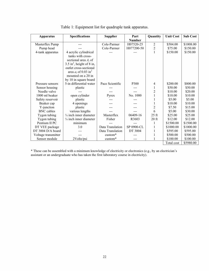
Table 1 is a list of all equipment needed to construct the apparatus, including their costs. Four

cylindrical tanks are mounted vertically on an acrylic board and are arranged in a symmetric 2 × 2 fashion as

shown in Fig. 1. A small hole is drilled at the bottom of each tank to channel the water from each tank to a

differential pressure sensor via a 3/16-inch tubing. MASTERFLEX tubings (S/No. 6409-16) transport water

between the tanks. Taking into account the maximum capacity of all 4 tanks (750 ml) and the dead volume

inside the entire length of the tubings, a 1000-ml cylindrical beaker is enough to store and recycle water for

the experiment. Two MASTERFLEX volumetric pumps are used. A 5-gallon tank immediately below the

apparatus contains any spillage or splashing from overflow in any of the 4 tanks.

A Y-junction is used to divide the flow such that water is channeled to a bottom level tank and the

upper level tank diagonal to it. This arrangement makes both levels in the bottom two tanks a function of

both pump flow rates. By adjusting the valve knob, the process can be operated so that one of the

multivariable transition zeros is in the right half plane, the left half plane, or switches between the two

planes in a stochastic time-varying manner.

The low cross-sectional area of the tanks makes level variations easy to see with the naked eye.

Hence students, teaching assistants, and instructors can assess the performance of the closed-loop system

with a glance. The tank heights are small, so that closed-loop controllers that perform poorly lead to

overflow in the tanks, which is an indication that the control system needs better tuning, an alternative

control structure, or the interactions need to be changed to make the process more controllable.

The visual programming control interface used in the laboratory [6] was modified for use with this

apparatus. The interface enables students with a minimum background in computer programming to make

changes in the control structures. This revised visual programming interface is available for download at a

web site [7]. Readers are referred to the references for more details.

3. Motivation for the Apparatus

There are several advantages to including a quadruple tank process experiment in an undergraduate

chemical engineering laboratory. One advantage is that the experiment can demonstrate a range of

interactions from slight to very strong. The apparatus allows students to investigate the extent to which a

decentralized controller is capable of controlling the process as the interactions increase. Students can also

implement partial or full decoupling as a first step to reduce process interactions. This enables students to

obtain hands-on experience in how decoupling can improve the closed-loop performance in some situations

(when there are some interactions, but not too strong), while having significant limitations when the

interactions become sufficiently strong [8].

The quadruple tank dynamics have an adjustable multivariable transition zero, whose position can

be in the left or right half plane, depending on the ratio of flow rates between the tanks. This enables

4

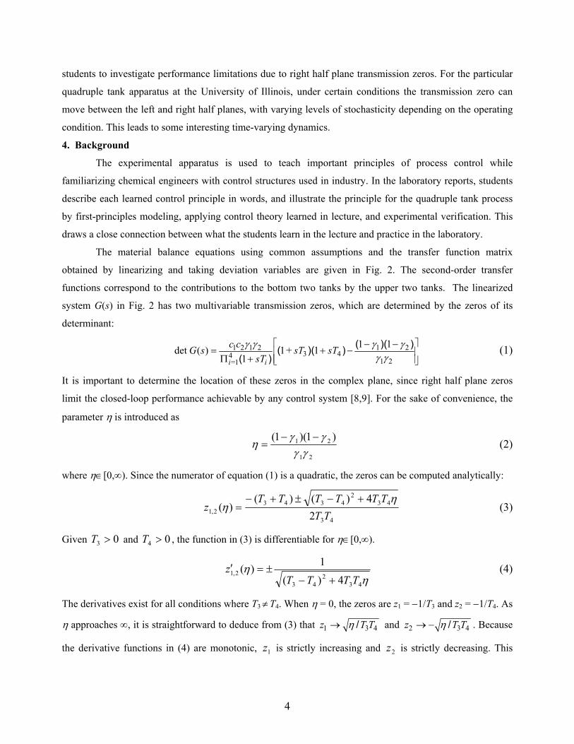
students to investigate performance limitations due to right half plane transmission zeros. For the particular

quadruple tank apparatus at the University of Illinois, under certain conditions the transmission zero can

move between the left and right half planes, with varying levels of stochasticity depending on the operating

condition. This leads to some interesting time-varying dynamics.

4. Background

The experimental apparatus is used to teach important principles of process control while

familiarizing chemical engineers with control structures used in industry. In the laboratory reports, students

describe each learned control principle in words, and illustrate the principle for the quadruple tank process

by first-principles modeling, applying control theory learned in lecture, and experimental verification. This

draws a close connection between what the students learn in the lecture and practice in the laboratory.

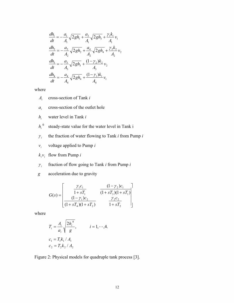
The material balance equations using common assumptions and the transfer function matrix

obtained by linearizing and taking deviation variables are given in Fig. 2. The second-order transfer

functions correspond to the contributions to the bottom two tanks by the upper two tanks. The linearized

system G(s) in Fig. 2 has two multivariable transmission zeros, which are determined by the zeros of its

determinant:

1 2 1 2 1 23 44

1 2=1

1 1det ( ) 1+ 11

( )( )( )( )( )

γ γ γ γγ γ

− −= + −

Π + ii

c cG s sT sTsT

(1)

It is important to determine the location of these zeros in the complex plane, since right half plane zeros

limit the closed-loop performance achievable by any control system [8,9]. For the sake of convenience, the

parameter η is introduced as

21

21 )1)(1(γγ

γγη

−−= (2)

where η∈[0,∞). Since the numerator of equation (1) is a quadratic, the zeros can be computed analytically:

43

432

43432,1 2

4)()()(

TTTTTTTT

zη

η+−±+−

= (3)

Given 03 >T and 04 >T , the function in (3) is differentiable for η∈[0,∞).

ηη

432

43

2,14)(

1)(TTTT

z+−

±=′ (4)

The derivatives exist for all conditions where T3 ≠ T4. When η = 0, the zeros are z1 = −1/T3 and z2 = −1/T4. As

η approaches ∞, it is straightforward to deduce from (3) that 1 3 4/η→z T T and 2 3 4/η→ −z T T . Because

the derivative functions in (4) are monotonic, 1z is strictly increasing and 2z is strictly decreasing. This

5

implies that the transmission zero 1z will cross from the left half plane to the right half plane with increasing

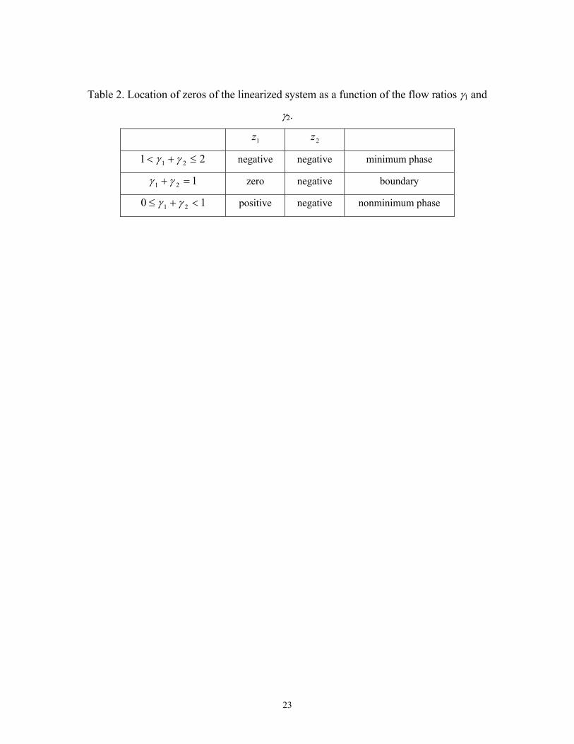
η. The crossing occurs at η = 1. With a little algebra, these results can be written in terms of the flow ratios

γ1 and γ2 as shown in Table 2. The process is minimum phase when the total flow to the lower tanks is

greater than the total flow to the upper tanks (1 < γ1 + γ2 < 2). The process is nonminimum phase (that is, has

a multivariable transmission zero in the right half plane) when the total flow to the lower tanks is smaller

than the total flow to the upper tanks. For operating conditions where the total flow to the upper tanks is

nearly the same as the total flow to the lower tanks, small variations in the flow rates due to nonideal

behavior in the tubing can cause the transmission zero to move between the two half planes in a stochastic

manner, in which case the process becomes uncontrollable [9]. More precisely, the steady-state determinant

of the transfer function (G(0) in Fig. 2) switches sign when 1 2γ γ+ crosses 1, indicating that it is impossible

to control the process with a linear time invariant feedback controller with integral action [9]. This is a

generalization of the single loop notion that the sign of the steady-state gain must be either consistently

positive or consistently negative for the process to be controllable with a linear feedback controller with

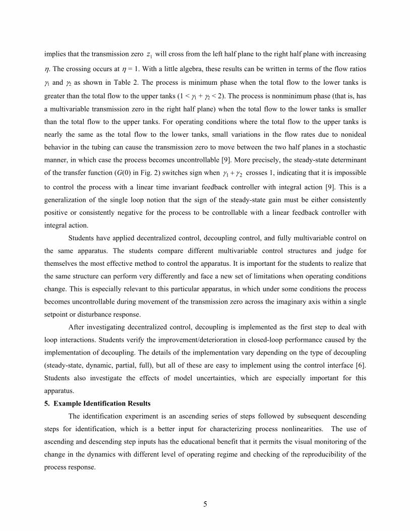
integral action. Students have applied decentralized control, decoupling control, and fully multivariable control on

the same apparatus. The students compare different multivariable control structures and judge for

themselves the most effective method to control the apparatus. It is important for the students to realize that

the same structure can perform very differently and face a new set of limitations when operating conditions

change. This is especially relevant to this particular apparatus, in which under some conditions the process

becomes uncontrollable during movement of the transmission zero across the imaginary axis within a single

setpoint or disturbance response.

After investigating decentralized control, decoupling is implemented as the first step to deal with

loop interactions. Students verify the improvement/deterioration in closed-loop performance caused by the

implementation of decoupling. The details of the implementation vary depending on the type of decoupling

(steady-state, dynamic, partial, full), but all of these are easy to implement using the control interface [6].

Students also investigate the effects of model uncertainties, which are especially important for this

apparatus.

5. Example Identification Results

The identification experiment is an ascending series of steps followed by subsequent descending

steps for identification, which is a better input for characterizing process nonlinearities. The use of

ascending and descending step inputs has the educational benefit that it permits the visual monitoring of the

change in the dynamics with different level of operating regime and checking of the reproducibility of the

process response.

6

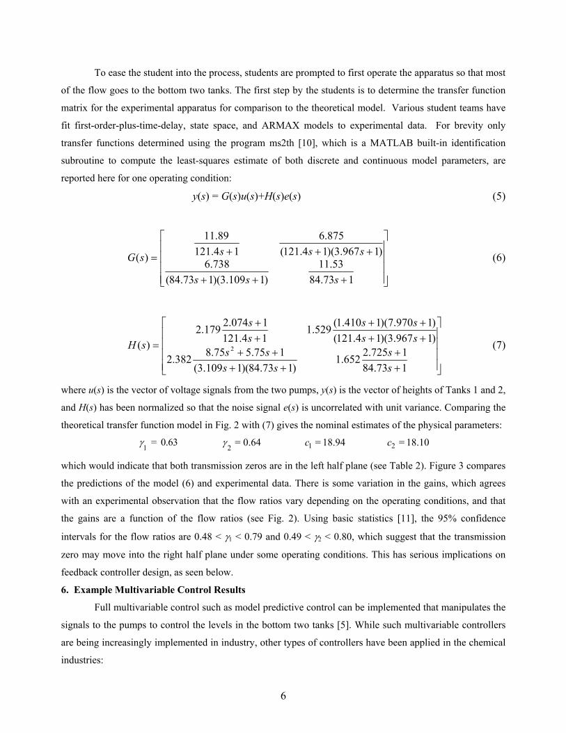
To ease the student into the process, students are prompted to first operate the apparatus so that most

of the flow goes to the bottom two tanks. The first step by the students is to determine the transfer function

matrix for the experimental apparatus for comparison to the theoretical model. Various student teams have

fit first-order-plus-time-delay, state space, and ARMAX models to experimental data. For brevity only

transfer functions determined using the program ms2th [10], which is a MATLAB built-in identification

subroutine to compute the least-squares estimate of both discrete and continuous model parameters, are

reported here for one operating condition:

y(s) = G(s)u(s)+H(s)e(s) (5)

+++

+++=

173.8453.11

)1109.3)(173.84(738.6

)1967.3)(14.121(875.6

14.12189.11

)(

sss

ssssG (6)

++

++++

++++

++

=

173.841725.2652.1

)173.84)(1109.3(175.575.8382.2

)1967.3)(14.121()1970.7)(1410.1(529.1

14.1211074.2179.2

)( 2

ss

ssss

ssss

ss

sH (7)

where u(s) is the vector of voltage signals from the two pumps, y(s) is the vector of heights of Tanks 1 and 2,

and H(s) has been normalized so that the noise signal e(s) is uncorrelated with unit variance. Comparing the

theoretical transfer function model in Fig. 2 with (7) gives the nominal estimates of the physical parameters:

1 = 0.63γ 2 = 0.64γ 1 = 18.94c 2 = 18.10c

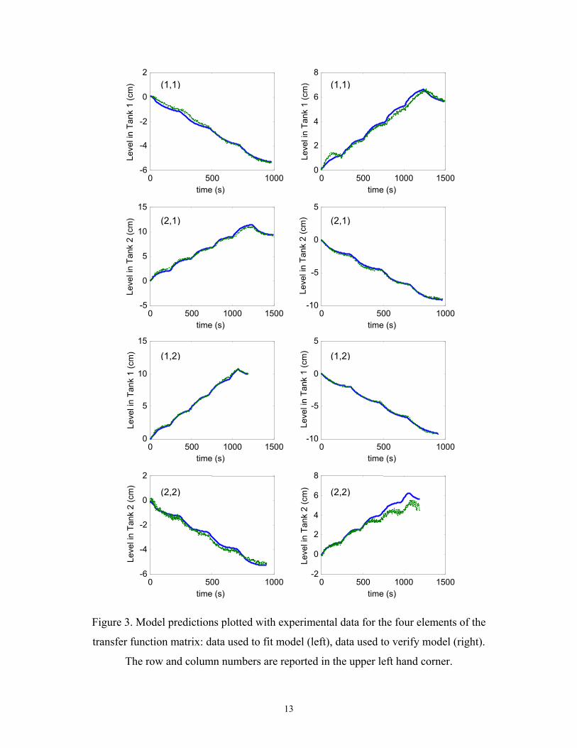
which would indicate that both transmission zeros are in the left half plane (see Table 2). Figure 3 compares

the predictions of the model (6) and experimental data. There is some variation in the gains, which agrees

with an experimental observation that the flow ratios vary depending on the operating conditions, and that

the gains are a function of the flow ratios (see Fig. 2). Using basic statistics [11], the 95% confidence

intervals for the flow ratios are 0.48 < γ1 < 0.79 and 0.49 < γ2 < 0.80, which suggest that the transmission

zero may move into the right half plane under some operating conditions. This has serious implications on

feedback controller design, as seen below.

6. Example Multivariable Control Results

Full multivariable control such as model predictive control can be implemented that manipulates the

signals to the pumps to control the levels in the bottom two tanks [5]. While such multivariable controllers

are being increasingly implemented in industry, other types of controllers have been applied in the chemical

industries:

7

1. Decentralized control: a noninteracting controller with single loop controllers designed for each tank.

Control loop 1 manipulates the flow through Pump 1 (via a voltage signal) to control the height of Tank

1, while Control loop 2 manipulates the flow through Pump 2 to control the height of Tank 2.

2. Partial decoupling followed by decentralized control.

3. Full decoupling followed by decentralized control.

Various students have implemented these control strategies on the quadruple tank process apparatus

during the past five years. Students implement up to three control strategies in a 7-week period, where the

scheduled lab time is 3 hours per week, and the lab report requirements include first-principles modeling,

analysis, and comparison between theory and experiment.

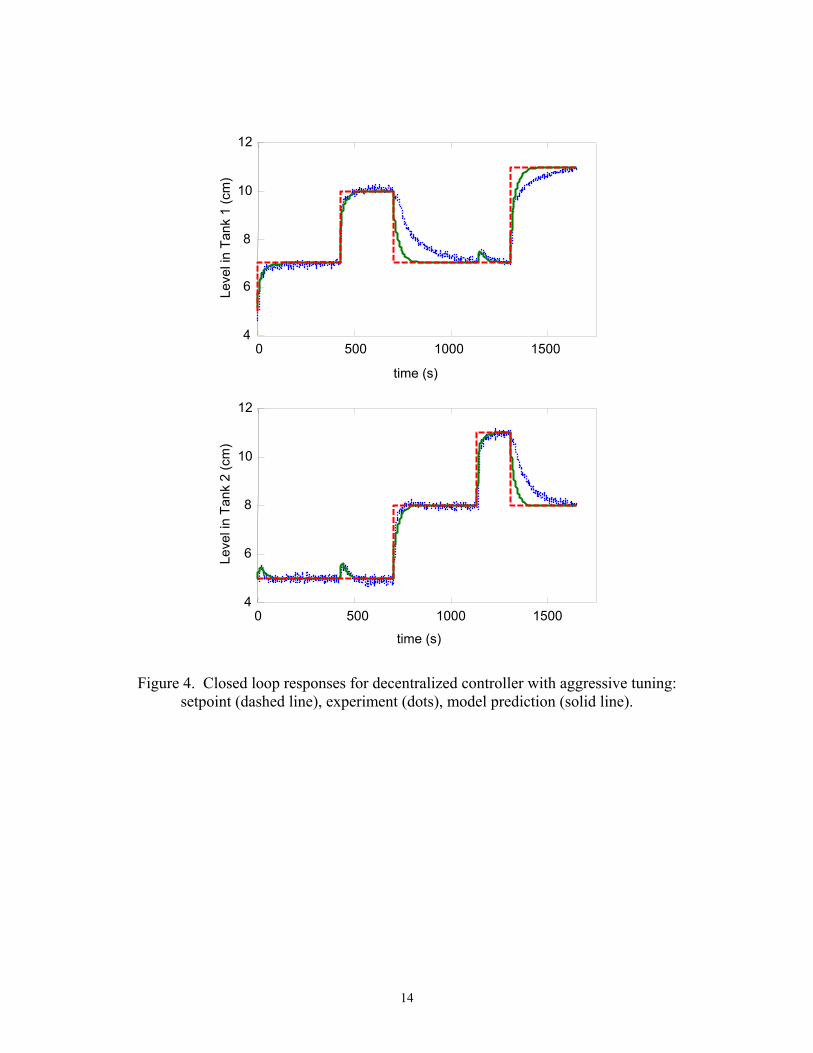
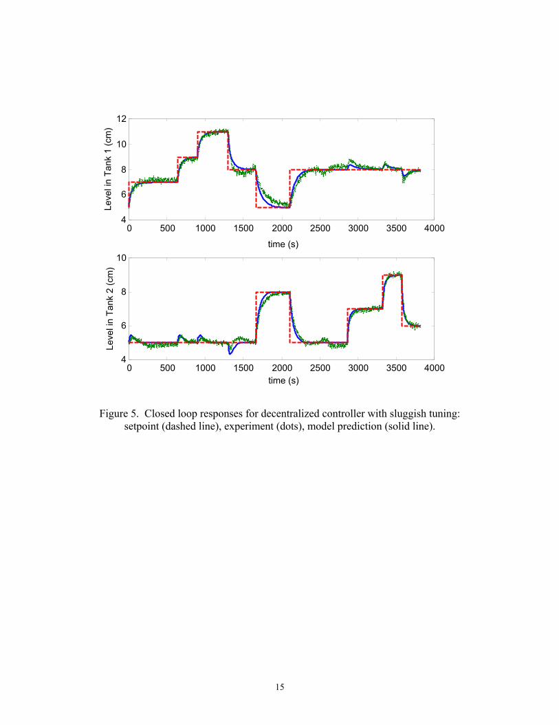
The relative gain for the nominal plant (6) is 1.5, which indicates that Pump i should be paired to the

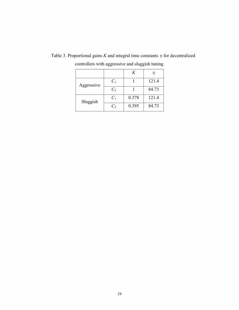
level in Tank I (8). Decentralized Internal Model Control Proportional-Integral (IMC-PI) controllers are

tuned to trade off robustness with performance [8,9,12] (see Table 3 and Figs. 4 and 5 for two levels of

tuning). Due to model uncertainties, the differences between model predictions and experiments are large

when the IMC-PI controllers are tuning too aggressively.

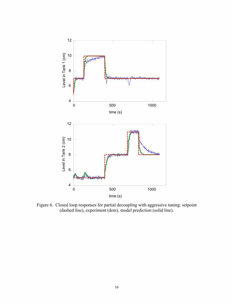
Implementing a partial dynamic decoupler and multiplying by the transfer function matrix in Fig. 2

gives

1 1

1

1 2 2 2

4 2 2 3 4

1 23 4

1 2

01+(1 ) Θ

(1+ )(1+ ) (1+ )(1+ )(1+ )(1 )(1 )1 1( )( )

=−

− −Θ = + + −

γ csT

G(s)γ c γ c

sT sT sT sT sTγ γsT sT γ γ

(8)

The transmission zeros are values of s in which Θ = 0 (see equation (1)). Both transmission zeros appear in

the second control loop. This results in a degradation of the closed-loop performance for the second control

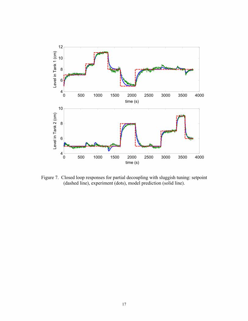
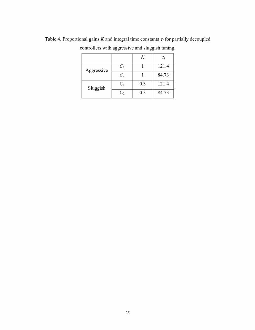
loop when one of these transmission zeros is in the right half plane. Using model (6), the results of tuning

IMC-PI controllers to trade off robustness with performance are shown in Table 4 and Figs. 6 and 7. Both

aggressive and sluggish tuning shows some interactions between the control loops, due to plant/model

mismatch. The differences between the model predictions and experimental data are larger for the aggressive

tuning.

While full dynamic decoupling is not common industrial practice, for educational purposes it is

useful to compare full dynamic decoupling with partial dynamic decoupling, to illustrate how full

decoupling can lead to worse closed loop performance than partial decoupling. Implementing a full dynamic

decoupler and multiplying by the transfer function matrix in Fig. 2 gives

8

+++Θ

+++Θ

=

)1)(1)(1(0

0)1)(1)(1()(ˆ

432

22

431

11

sTsTsTc

sTsTsTc

sG γ

γ

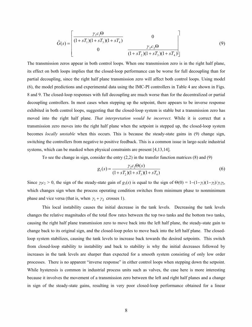
(9)

The transmission zeros appear in both control loops. When one transmission zero is in the right half plane,

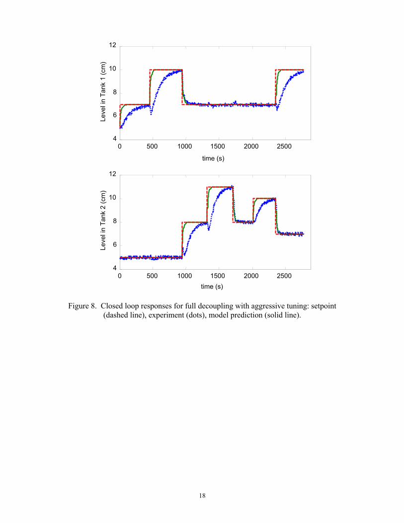
its effect on both loops implies that the closed-loop performance can be worse for full decoupling than for

partial decoupling, since the right half plane transmission zero will affect both control loops. Using model

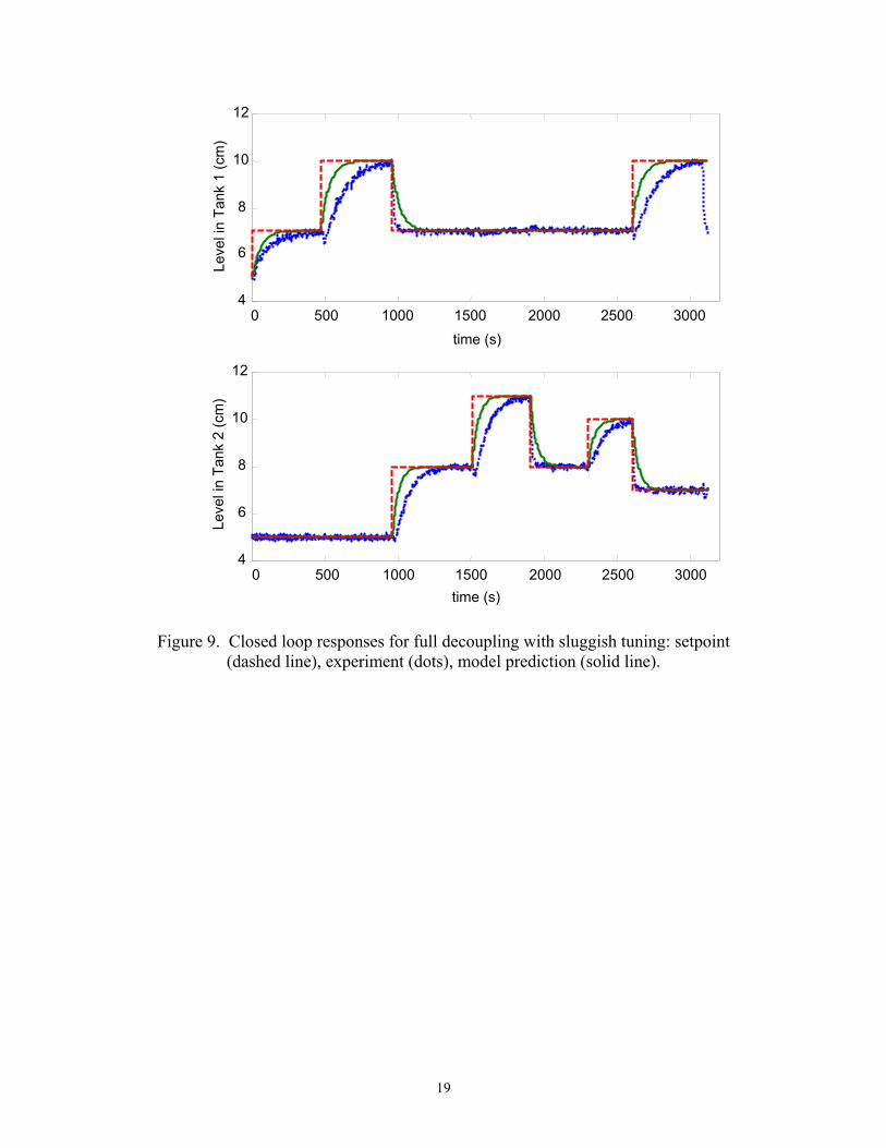
(6), the model predictions and experimental data using the IMC-PI controllers in Table 4 are shown in Figs.

8 and 9. The closed-loop responses with full decoupling are much worse than for the decentralized or partial

decoupling controllers. In most cases when stepping up the setpoint, there appears to be inverse response

exhibited in both control loops, suggesting that the closed-loop system is stable but a transmission zero has

moved into the right half plane. That interpretation would be incorrect. While it is correct that a

transmission zero moves into the right half plane when the setpoint is stepped up, the closed-loop system

becomes locally unstable when this occurs. This is because the steady-state gains in (9) change sign,

switching the controllers from negative to positive feedback. This is a common issue in large-scale industrial

systems, which can be masked when physical constraints are present [4,13,14].

To see the change in sign, consider the entry (2,2) in the transfer function matrices (8) and (9)

2 21

2 3 4

( )( )(1 )(1 )(1 )

γ Θ=

+ + +c sg s

sT sT sT (6)

Since γ2c2 > 0, the sign of the steady-state gain of g1(s) is equal to the sign of Θ(0) = 1−(1−γ1)(1−γ2)/γ1γ2,

which changes sign when the process operating condition switches from minimum phase to nonminimum

phase and vice versa (that is, when 1 2γ γ+ crosses 1).

This local instability causes the initial decrease in the tank levels. Decreasing the tank levels

changes the relative magnitudes of the total flow rates between the top two tanks and the bottom two tanks,

causing the right half plane transmission zero to move back into the left half plane, the steady-state gain to

change back to its original sign, and the closed-loop poles to move back into the left half plane. The closed-

loop system stabilizes, causing the tank levels to increase back towards the desired setpoints. This switch

from closed-loop stability to instability and back to stability is why the initial decreases followed by

increases in the tank levels are sharper than expected for a smooth system consisting of only low order

processes. There is no apparent “inverse response” in either control loops when stepping down the setpoint.

While hysteresis is common in industrial process units such as valves, the case here is more interesting

because it involves the movement of a transmission zero between the left and right half planes and a change

in sign of the steady-state gains, resulting in very poor closed-loop performance obtained for a linear

9

controller.1 For this particular valve knob setting, the full decoupling controller induces this behavior more

readily than the decentralized or partial decoupling controller. This illustrates the important point that, when

interactions are large enough, decoupling control can do more harm than good [8,9]. Full decoupling control

has increased sensitivity to uncertainties in the transfer function model, which causes the ratios of the total

flow rates in the bottom tanks and top tanks to vary more than for the other controllers. If the valve knob is

shifted so that the transmission zero easily moves between the right and left half planes for the whole

operating range (instead of only for some conditions, as in Figs. 8 and 9), then good setpoint tracking is

unobtainable by a linear controller, no matter how sophisticated [9]. The second important point is that

hysteresis effects are common in industrial control loops, and should be considered when troubleshooting.

The third point is that the cause of unexpected dynamic behavior in control loops is often more subtle than

what is often first assumed. But such phenomena can be understood with some thinking and judicious

application of undergraduate-level process control analysis tools. This understanding is needed to determine

whether a particular control problem can be resolved by better controller tuning, a different control structure,

changing the process design, or by changing the operating conditions.

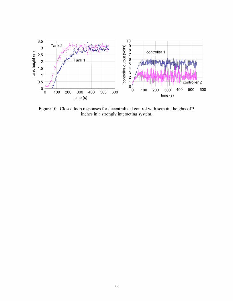
For the next experiment, the quadruple tank process was made more interacting by using the Y-

junctions to increase the proportion of flow to the top tanks. Closed-loop responses with decentralized

control are shown in Fig. 10. Due to the higher interactions, as well as some nonlinear effects, the closed-

loop responses are highly oscillatory around the setpoints. The student was unable to obtain controller

tuning parameters that would stabilize the closed-loop system when either steady-state or dynamic

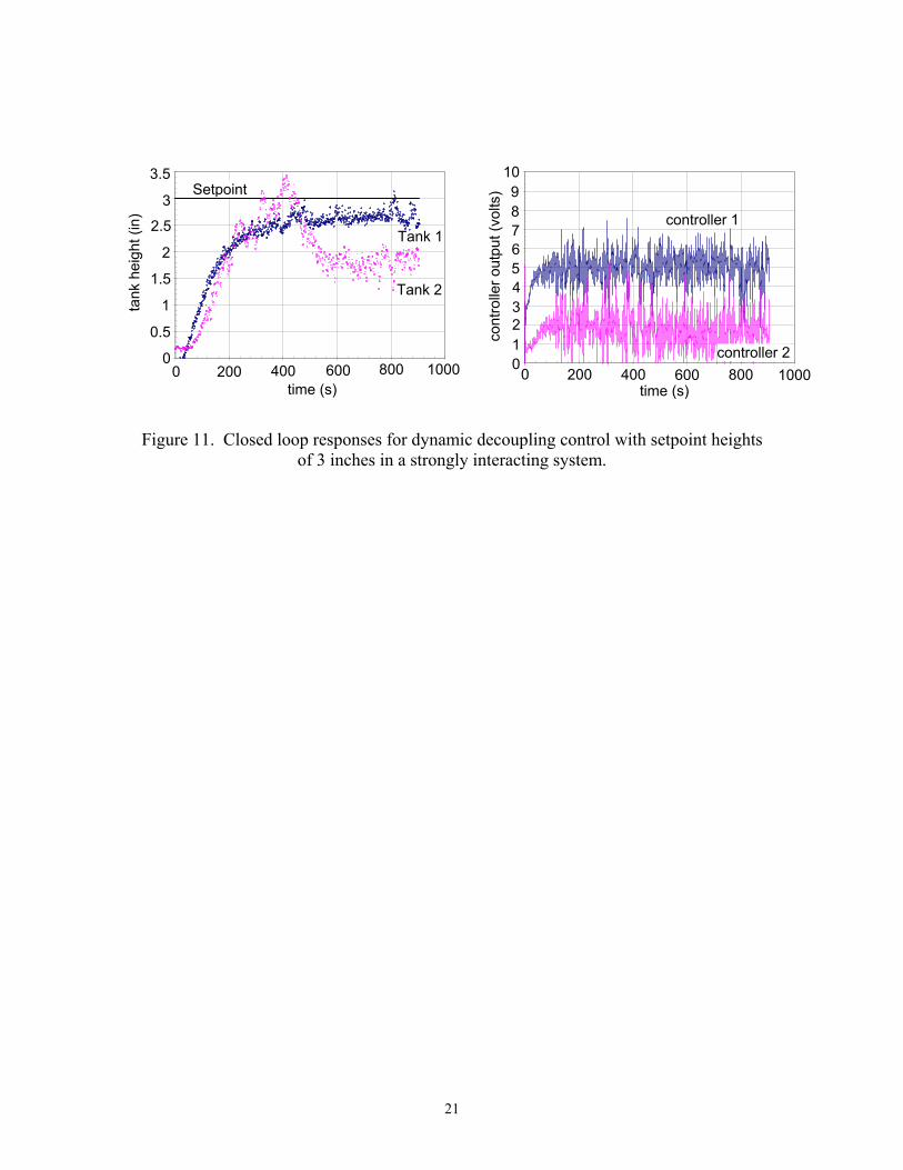
decoupling was used. The best closed-loop response obtained by dynamic decoupling is shown in Fig. 11.

The initial closed-loop performance was acceptable up to 200 s. However, the level in Tank 2 deviated from

the setpoint for t > 400 s, indicating that the closed-loop system was not locally asymptotically stable. In

addition, there was a consistent steady-state offset exhibited by the level in Tank 1. Again, this illustrates to

students that a process that is designed poorly can be difficult or impossible to control.

Different student teams are given different valve settings in the Y-junctions, and students are

encouraged to share their results with other student teams. Students who consistently have >80% of the flow

going to the bottom tanks observe that decoupling control can provide better closed-loop performance than

multiloop control. Decoupling control performs worse than decentralized control when the interactions are

increased. When the total flows to the top and bottom tanks are equal or nearly equal, no linear controller

can provide acceptable closed-loop performance.

1 Although the essence of the argument is valid, for the student’s sake this interpretation involves some simplification, since the real system is nonlinear.

10

7. Conclusions

A 4-tank apparatus was introduced in which a multivariate transmission zero can cross the

imaginary axis during a single closed loop response, which is used to illustrate the effects of time-varying

dynamics, changes in the sign of the steady-state gain, and hysteresis. Example student results illustrated

how the apparatus is used to teach many important points that are ignored in most process control lectures

and laboratories: (1) the effect of time-varying dynamics should be considered when designing control

systems, (2) the sign of the steady-state gain should always be considered when designing control systems

for multivariable processes, (3) the cause of unexpected dynamic behavior in control loops is often more

subtle than what is first assumed, (4) under some conditions, full decoupling can lead to significantly worse

performance than partial decoupling, (5) decoupling control can do more harm than good, and (6) hysteresis

effects should be considered when troubleshooting control problems. This level of understanding is needed

for students to select the proper multivariable control structure and to determine whether a particular control

problem can be addressed by better controller tuning, a different control structure, changing the process

design, or by changing the operating conditions.

Although not reported here, the apparatus has been used to implement partial and full steady-state

decoupling, to compare with dynamic decoupling. Also, it would be educationally valuable to investigate

the development of feedback linearizing controllers to enable a single controller to provide good

performance for a wider range of operating conditions [15].

8. Acknowledgment

The University of Illinois IBHE program is acknowledged for support of this project.

11

Literature Cited

1. D. J. Cooper, “Picles™: A Simulator for ‘Virtual World’ Education and Training in Process

Dynamics and Control”, Computer Applications in Engineering Education, 4, 207-215, 1996.

2. F. J. Doyle III, E. P. Gatzke, and R. S. Parker, Process Control Modules: A Software Laboratory for

Control Design, Prentice Hall, Upper Saddle River, NJ, 2000.

3. K. H. Johansson, “The Quadruple-Tank Process: A Multivariable Laboratory Process with an

Adjustable zero”, IEEE Trans. on Control Systems Technology, 8, 456-465, 2000.

4. A. P. Featherstone and R. D. Braatz, “Integrated Robust Identification and Control of Large Scale

Processes”, Ind. Eng. Chem. Res., 37, 97-106, 1998.

5. E. P. Gatzke, E. S. Meadows, C. Wang, and F. J. Doyle III, “Model Based Control of a Four-tank

System”, Computers and Chemical Engineering, 24, 1503-1509, 2000.

6. R. D. Braatz and M. R. Johnson. Process Control Laboratory Education Using a Graphical Operator

Interface. Computer Applications in Engineering Education, 6, 151-155, 1998.

7. http://brahms.scs.uiuc.edu

8. B. A. Ogunnaike and W. H. Ray, Process Dynamics, Modeling, and Control, Oxford University

Press, New York, 1994.

9. M. Morari and E. Zafiriou, Robust Process Control, Prentice Hall, Englewood Cliffs, NJ, 1989.

10. L. Ljung, System Identification Toolbox: User’s Guide, The Mathworks Inc., Natick, MA, 1995.

11. L. Ljung, System Identification: Theory for the User, Prentice Hall, Englewood Cliffs, NJ, 1987.

12. R. D. Braatz, Internal Model Control. In W. S. Levine, editor, Control Systems Fundamentals, pages

215-224. CRC Press, Boca Raton, FL, 2000.

13. E. L. Russell and R. D. Braatz, “The Average-case Identifiability and Controllability of Large Scale

Systems”, J. of Process Control, 12, 823-829, 2002.

14. G. Nunes, S. Kincal, and O. D. Crisalle, “Stability Analysis of Multivariable Predictive Control – A

Polynomial Approach”, Proc. of the American Control Conf., 3, 2424-2429, 2001.

15. B. A. Ogunnaike, “Controller Design for Nonlinear Process Systems via Variable Transformations”,

Ind. Eng. Chem. Proc. Des. Dev., 25, 241-248, 1986.

11

Safety Overflow (only used if leaks or splashing occurs)

Figure 1: Schematic of the quadruple tank process apparatus. To simplify the figure, not shown are a tube between Tank 3 and Tank 1, a tube between Tank 4 and Tank 2, a tube from Tank 1 to the water reservoir, a tube between Tank 2 and the water reservoir, and a

lid on the water reservoir. These tubes and lid are used to reduce evaporation.

Data AcquisitionHardware & Computer

Pump 1 Pump 2Tank 1 Tank 2

Tank 3 Tank 4

F1 F2

γ1F1

(1-γ1)F1 (1-γ2)F2

γ2F2

Water Reservoir

12

14

114

4

44

23

223

3

33

22

224

2

42

2

22

11

113

1

31

1

11

)1(2

)1(2

22

22

vA

kghAa

dtdh

vA

kghAa

dtdh

vAkgh

Aagh

Aa

dtdh

vAkgh

Aagh

Aa

dtdh

γ

γ

γ

γ

−+−=

−+−=

++−=

++−=

where

iA cross-section of Tank i

ia cross-section of the outlet hole

ih water level in Tank i

ih 0 steady-state value for the water level in Tank i

iγ the fraction of water flowing to Tank i from Pump i

iv voltage applied to Pump i

iivk flow from Pump i

iγ fraction of flow going to Tank i from Pump i

g acceleration due to gravity

+++−

++−

+=

2

22

24

21

13

12

1

11

1)1)(1()1(

)1)(1()1(

1)(

sTc

sTsTc

sTsTc

sTc

sG γγ

γγ

where

.4,,1,2 0

== igh

aA

T i

i

ii

1111 / AkTc =

2222 / AkTc = Figure 2: Physical models for quadruple tank process [3].

13

Figure 3. Model predictions plotted with experimental data for the four elements of the

transfer function matrix: data used to fit model (left), data used to verify model (right).

The row and column numbers are reported in the upper left hand corner.

0 500 1000 15000

5

10

15

time (s)

Leve

l in

Tank

1 (c

m)

0 500 1000 -10

-5

0

5

time (s)

Leve

l in

Tank

1 (c

m)

0 500 1000 1500 -2

0

2

4

6

8

time (s)

Leve

l in

Tank

2 (c

m)

0 500 1000-6

-4

-2

0

2

time (s)

Leve

l in

Tank

2 (c

m)

0 500 1000-6

-4

-2

0

2

time (s)

Leve

l in

Tank

1 (c

m)

0 500 1000 1500 0

2

4

6

8

time (s)

Leve

l in

Tank

1 (c

m)

0 500 1000 -10

-5

0

5

time (s)

Leve

l in

Tank

2 (c

m)

0 500 1000 1500-5

0

5

10

15

time (s)

Leve

l in

Tank

2 (c

m)

(1,1) (1,1)

(2,1) (2,1)

(1,2)(1,2)

(2,2) (2,2)

14

Figure 4. Closed loop responses for decentralized controller with aggressive tuning: setpoint (dashed line), experiment (dots), model prediction (solid line).

0 500 1000 15004

6

8

10

12

Leve

l in

Tank

1 (c

m)

0 500 1000 15004

6

8

10

12

Leve

l in

Tank

2 (c

m)

time (s)

time (s)

15

Figure 5. Closed loop responses for decentralized controller with sluggish tuning: setpoint (dashed line), experiment (dots), model prediction (solid line).

0 500 1000 1500 2000 2500 3000 3500 4000 4

6

8

10

12 Le

vel i

n Ta

nk 1

(cm

)

0 500 1000 1500 2000 2500 3000 3500 4000 4

6

8

10

Leve

l in

Tank

2 (c

m)

time (s)

time (s)

16

Figure 6. Closed loop responses for partial decoupling with aggressive tuning: setpoint (dashed line), experiment (dots), model prediction (solid line).

0 500 10004

6

8

10

12

Leve

l in

Tank

1 (c

m)

0 500 10004

6

8

10

12

Leve

l in

Tank

2 (c

m)

time (s)

time (s)

17

Figure 7. Closed loop responses for partial decoupling with sluggish tuning: setpoint (dashed line), experiment (dots), model prediction (solid line).

0 500 1000 1500 2000 2500 3000 3500 40004

6

8

10

12

Leve

l in

Tank

1 (c

m)

0 500 1000 1500 2000 2500 3000 3500 40004

6

8

10

Leve

l in

Tank

2 (c

m)

time (s)

time (s)

18

Figure 8. Closed loop responses for full decoupling with aggressive tuning: setpoint

(dashed line), experiment (dots), model prediction (solid line).

0 500 1000 1500 2000 2500 4

6

8

10

12

Leve

l in

Tank

1 (c

m)

0 500 1000 1500 2000 2500 4

6

8

10

12

Leve

l in

Tank

2 (c

m)

time (s)

time (s)

19

re 9. Full decoupling with sluggish tuning: setpoint (dashed line), experiment (dots),

model prediction (solid line).

Figure 9. Closed loop responses for full decoupling with sluggish tuning: setpoint (dashed line), experiment (dots), model prediction (solid line).

0 500 1000 1500 2000 2500 3000 4

6

8

10

12

Leve

l in

Tank

1 (c

m)

0 500 1000 1500 2000 2500 3000 4

6

8

10

12

Leve

l in

Tank

2 (c

m)

time (s)

time (s)

20

Figure 10. Closed loop responses for decentralized control with setpoint heights of 3

inches in a strongly interacting system.

0

0.5

1

1.5

2

2.5

3

3.5

0 100 200 300 400 500 600time (s)

tank

hei

ght (

in)

Tank 2

0123456789

10

0 100 200 300 400 500 600time (s)

cont

rolle

r out

put (

volts

)

controller 1

Tank 1

controller 2

21

Figure 11. Closed loop responses for dynamic decoupling control with setpoint heights of 3 inches in a strongly interacting system.

0

0.5

1

1.5

2

2.5

3

3.5

0 200 400 600 800 1000time (s)

tank

hei

ght (

in)

Tank 1

Tank 2

Setpoint

0123456789

10

0 200 400 600 800 1000time (s)

cont

rolle

r out

put (

volts

)

controller 1

controller 2

22

Table 1: Equipment list for quadruple tank apparatus.

Apparatus Specifications Supplier Part Number

Quantity Unit Cost Sub Cost

Masterflex Pump --- Cole-Parmer H07520-25 2 $504.00 $1008.00 Pump head --- Cole-Parmer H077200-50 2 $75.00 $150.00

4-tank apparatus 4 acrylic cylindrical tanks with cross-

sectional area Ai of 3.5 in2, height of 8 in, outlet cross-sectional

area ai of 0.03 in2 mounted on a 20 in

by 10 in square board

--- --- 1 $150.00 $150.00

Pressure sensors 5-in differential water Pace Scientific P300 4 $200.00 $800.00 Sensor housing plastic --- --- 1 $50.00 $50.00 Needle valve --- --- --- 2 $10.00 $20.00

1000 ml beaker open cylinder Pyrex No. 1000 1 $10.00 $10.00 Safety reservoir plastic --- --- 1 $5.00 $5.00

Beaker cap 4 openings --- --- 1 $10.00 $10.00 Y-junction plastic --- --- 2 $7.50 $15.00 BNC cables various lengths --- --- 6 $5.00 $30.00

Tygon tubing ¼ inch inner diameter Masterflex 06409-16 25 ft $25.00 $25.00 Tygon tubing ¼ inch inner diameter Fisher R3603 20 ft $12.00 $12.00 Pentium II PC minimum --- --- 1 $1500.00 $1500.00

DT VEE package 3.0 Data Translation SP 0900-CL 1 $1000.00 $1000.00 DT 3004 D/A board --- Data Translation DT 3004 1 $595.00 $595.00 Voltage transmitter --- custom* --- 1 $500.00 $500.00

Sensor module 2Voltz/psi custom* --- 1 $100.00 $100.00 Total cost $5980.00

* These can be assembled with a minimum knowledge of electricity or electronics (e.g., by an electrician’s assistant or an undergraduate who has taken the first laboratory course in electricity).

23

Table 2. Location of zeros of the linearized system as a function of the flow ratios γ1 and

γ2.

1z 2z

21 21 ≤+< γγ negative negative minimum phase

121 =+ γγ zero negative boundary

10 21 <+≤ γγ positive negative nonminimum phase

24

Table 3. Proportional gains K and integral time constants τI for decentralized

controllers with aggressive and sluggish tuning.

K τI

C1 1 121.4 Aggressive

C2 1 84.73

C1 0.378 121.4 Sluggish

C2 0.395 84.73

25

Table 4. Proportional gains K and integral time constants τI for partially decoupled

controllers with aggressive and sluggish tuning.

K τI

C1 1 121.4 Aggressive

C2 1 84.73

C1 0.3 121.4 Sluggish

C2 0.3 84.73