Embed Size (px)
Citation preview

A pseudo-matched filter for chaosSeth D. Cohen and Daniel J. Gauthier Citation: Chaos 22, 033148 (2012); doi: 10.1063/1.4754437 View online: http://dx.doi.org/10.1063/1.4754437 View Table of Contents: http://chaos.aip.org/resource/1/CHAOEH/v22/i3 Published by the American Institute of Physics. Related ArticlesA heuristic method for identifying chaos from frequency content Chaos 22, 013136 (2012) Stabilization of chaos systems described by nonlinear fractional-order polytopic differential inclusion Chaos 22, 013120 (2012) Robust adaptive synchronization for a general class of uncertain chaotic systems with application to Chua’scircuit Chaos 21, 043134 (2011) Plykin type attractor in electronic device simulated in MULTISIM Chaos 21, 043105 (2011) How to combine independent data sets for the same quantity Chaos 21, 033102 (2011) Additional information on ChaosJournal Homepage: http://chaos.aip.org/ Journal Information: http://chaos.aip.org/about/about_the_journal Top downloads: http://chaos.aip.org/features/most_downloaded Information for Authors: http://chaos.aip.org/authors
Downloaded 03 Oct 2012 to 152.3.68.83. Redistribution subject to AIP license or copyright; see http://chaos.aip.org/about/rights_and_permissions
A pseudo-matched filter for chaos
Seth D. Cohen and Daniel J. GauthierDepartment of Physics, Duke University, Durham, North Carolina 27708, USA
(Received 4 April 2012; accepted 6 September 2012; published online 26 September 2012)
A matched filter maximizes the signal-to-noise ratio of a signal. In the recent work of Corron
et al. [Chaos 20, 023123 (2010)], a matched filter is derived for the chaotic waveforms produced
by a piecewise-linear system. This system produces a readily available binary symbolic
dynamics that can be used to perform correlations in the presence of large amounts of noise using
the matched filter. Motivated by these results, we describe a pseudo-matched filter, which
operates similarly to the original matched filter. It consists of a notch filter followed by a
first-order, low-pass filter. We compare quantitatively the matched filter’s performance to that of
our pseudo-matched filter using correlation functions. On average, the pseudo-matched filter
performs with a correlation signal-to-noise ratio that is 2.0 dB below that of the matched filter.
Our pseudo-matched filter, though somewhat inferior in comparison to the matched filter, is
easily realizable at high speed (>1 GHz) for potential radar applications. VC 2012 AmericanInstitute of Physics. [http://dx.doi.org/10.1063/1.4754437]
Recently, Corron et al. developed an analog matched fil-
ter that uses the digital symbolic dynamics of a piecewise-
linear chaotic system. This matched filter for chaos is
derived from the analytic solution of their uniquely
designed chaotic system. However, the majority of cha-
otic systems do not have analytically solvable dynamics.
In order to extend the ideas presented by Corron et al. to
other systems with symbolic dynamics, this problem must
be approached empirically, rather than analytically. To
do so, we derive a pseudo-matched filter for this particu-
lar piecewise-linear system. The matched filter, which is
optimal, serves as a baseline to benchmark the pseudo-
matched filter’s performance. Quantitative comparisons
are established using the two filters in a chaos radar
application. Our hope is that, based on our analysis of the
chaos in the Fourier and time domains, filtering techni-
ques can be developed for applications that use the sym-
bolic dynamics of higher dimensional chaotic systems in
the presence of noise.
I. INTRODUCTION
A conventional radar system measures the distances of
targets in the field of view using a signal source, a transmit-
ter, and a receiver. In Fig. 1, a radar transmitter broadcasts
a signal u(t) from the source toward an intended target, and
the receiver detects a version of the transmitted signal that
is reflected off of the target. Prior to transmission, a copy of
the radar signal’s information is digitally sampled and
stored as sn. The received signal v(t), which picks up envi-
ronmental noise, is filtered and correlated with sn. Typical
radar signals are non-repeating in order to avoid multiple
points of correlation and, therefore, the correlation will
peak only when the transmitted and received signals are
aligned. Using the time of the output peak in the correla-
tion, the measured range from the transmitter to the target
is determined.
The performance of a radar is determined by its ability
to identify the correlation time between the transmitted and
received signal. In the correlation function, the width of the
peak scales inversely with the bandwidth of the transmitted
signal and sets the spatial resolution of the radar. In addition,
the height of the correlation peak above the noise floor, also
known as signal-to-noise ratio (SNR), is determined by the
length of the transmitted and sampled waveforms as well as
the noise from the environment. Thus, the digital storage
capacity of the radar sets the maximum SNR in the correla-
tion measurement. State-of-the-art radar systems use high-
frequency, broadband signals, where the digital sampling
and storage of the signals can be costly. These radars must
balance the bandwidth and cost of the systems design while
maintaining its performance.
A simple example of an inexpensive, non-repeating,
broadband signal source is amplified electrical noise. In the
past, electrical noise has been used by radar systems to per-
form ranging measurements.1,2 The high bandwidth of these
noise generators yields high-resolution ranging information
but requires fast sampling and large data storage capacities.
Some recent techniques have been proposed to minimize the
necessary sampling capacity of noise radars using analog
delay lines for signal storage.3 But these methods limit the
ranging capabilities of the radar.
Various deterministic signal sources have been studied in
efforts to minimize the necessary data storage rate and
capacity of a radar. As one example, pseudo-random binary
sequences (PRBSs) are often used as a radar signal sources.
To be implemented as a radar signal source, a PRBS is
up-converted to a suitable frequency band before transmitting
and then down-converted at the receiver before correlation.4,5
The main advantage of a PRBS is the ability to use one-bit
digital samplings of the binary sequences, thereby requiring
low amounts of data-storage capacity. This allows for longer
sequences of the transmitted waveform to be stored, thus
enhancing the radar’s SNR without increasing the cost of the
1054-1500/2012/22(3)/033148/10/$30.00 VC 2012 American Institute of Physics22, 033148-1
CHAOS 22, 033148 (2012)
Downloaded 03 Oct 2012 to 152.3.68.83. Redistribution subject to AIP license or copyright; see http://chaos.aip.org/about/rights_and_permissions

system. The main disadvantage of a PRBS is that it requires
computational power to generate and its sequence eventually
repeats, which ultimately limits its performance. Many other
radar concepts like this one exist, each with advantages and
disadvantages, and today the radar community continues to
develop broadband signal sources.6,7
One novel approach to a radar is to use chaotic wave-
form generators, which are believed to have several proper-
ties that make them ideally suited as signal sources for radar
applications.8 One defining feature of a chaotic system is
that it can generate a signal that does not repeat in time. Cha-
otic signals are also often inherently broadband. High-speed
chaos has been observed in optical and electronic systems
with frequency bandwidths that stretch across several giga-
hertz.9–11 Such broadband chaos has been studied for its
applications in high-resolution ranging and in imaging.12–15
These applications use the non-repeating aspects of the high-
speed chaos.
However, conventional chaos radars do not take full
advantage of the chaotic signal source. In addition to produc-
ing broadband, non-repeating signals, chaotic systems are
deterministic and extremely sensitive to small perturbations.
By not using these properties, chaos radars add no benefit
over noise radars, requiring high-sampling to perform corre-
lations. In addition, many modern proposals for chaos-based
applications implement chaos using digital synthesis,16
which requires digital processors and up/down-conversion
for radar. Thus, to take full advantage of chaotic systems in a
radar application, a chaos radar needs to benefit from the
determinism or sensitivity of analog chaos in addition to its
noise-like properties.
Recently, Corron et al. proposed a novel chaos radar
concept that uses the analog dynamics produced by a
piecewise-linear harmonic oscillator.17–19 It produces simul-
taneously an analog chaotic signal and a binary switching
state (symbolic dynamics) that completely characterizes its
chaotic dynamics. In the proposed radar, the chaotic signal
serves as the signal source (see Fig. 1) and is transmitted,
while a copy of a switching state is stored using a one-bit
digital sampling. For a radar receiver, Corron et al. derived
the analytical form of a filter that is matched to a basis func-
tion, which is inherently encoded in the chaos produced by
the system. A matched filter is a linear operation that opti-
mizes the SNR of a signal in the presence of additive white
Gaussian noise (AWGN).20 Their matched filter, when
applied to the received signal, can be used in conjuction with
the stored symbolic dynamics in the correlation operation of
Fig. 1. This technique uses deterministic aspects of the
chaos, making it an improvement over a noise radar. With
reduced data storage and an optimal SNR, their architecture
could effectively reduce the cost of a radar system.
Corron et al. implement their piecewise-linear design
using an inductance-resistance-capacitance (LRC) oscillator
that operates in the kHz frequency range.18 It is difficult to
realize a high-frequency version (>1 GHz) of this system
because of parasitic capacitances and inductances associated
with high-speed electronics.21 In addition, at high-speeds,
there are inherent time delays in the propagation of signals
in LRC circuits.22 As it stands, there is no high-frequency
realization of the piecewise-linear system from Ref. 18 or
the associated matched filter. In order to have resolutions
that are comparable to state-of-the art radar systems, the
waveforms and switching states produced by this chaotic
system must be scaled to higher-frequencies and to broader
bandwidths. Thus, techniques for simplifying the design by
Corron et al. and increasing its speed are of interest.
To begin simplifying their approach, we present a set of
standard filters (first order low-pass filter and notch filter).
Cascading these standard filters allows us to realize a pseudo-
matched filter for the chaos produced by the piecewise-linear
harmonic oscillator. We define a pseudo-matched filter as a
sub-optimal linear operation (when compared to the matched
filter) that performs comparably to the matched filter for the
system. As we will show, the pseudo-matched filter is empiri-
cally derived from the observed spectral properties of the
chaos and is suited to perform correlations with the system’s
symbolic dynamics for applications like chaos radar.
In addition, as a first step toward a high-frequency
implementation of Corron et al.’s system, we present a sim-
ple, high-speed design for the pseudo-matched filter. The
design includes filters that operate at high-frequencies, which
are inexpensive, well characterized, and readily available.
Motivated by the chaos-based radar system proposed by Ref.
19, we are interested in high-speed architectures that also
take advantage of a chaotic system’s symbolic dynamics.
Our pseudo-matched filter for chaos shows that the approach
by Corron et al. does not need an analytically derived filter
and can benefit from integrating readily available filters for
radar applications.
II. MATCHED FILTER REVIEW
To motivate our analysis, we briefly review the charac-
teristics of the chaotic system and matched filter presented in
Ref. 18 within the context of a radar application. Consider a
harmonic oscillator with negative damping �b and with a
piecewise-constant driving term s(t) whose behavior is gov-
erned by the differential equation
FIG. 1. Example chaos radar. A signal u(t) is transmitted to measure target
distances and stored digitally as sn. The received signal v(t) is filtered and
correlated with sn. The correlation output vðtÞ peaks at time t ¼ 2spd þ sf ,
where spd is the propagation delay from the radar to the target and sf is the
delay through the filter.
033148-2 S. D. Cohen and D. J. Gauthier Chaos 22, 033148 (2012)
Downloaded 03 Oct 2012 to 152.3.68.83. Redistribution subject to AIP license or copyright; see http://chaos.aip.org/about/rights_and_permissions

€uðtÞ � 2b _uðtÞ þ ðx2o þ b2ÞðuðtÞ � sðtÞÞ ¼ 0; (1)
together with a guard condition on the output variable u(t)that switches the sign of s(t)
sðtÞ ¼ 1; if uðt�Þ � 0
�1; if uðt�Þ < 0;
�(2)
at times t� where _uðt�Þ ¼ 0.
Figure 2 shows a time series of the variables u(t) and
s(t) with the parameters xo ¼ 2p and b ¼ lnð2Þ. We inte-
grate Eqs. (1) and (2) using MATLAB’s ODE45, where the
switching condition is monitored using the integrator’s
event-detection algorithm. The attractor for this system is
low dimensional and is plotted in Fig. 2(b). The dynamics
can also be viewed as a chaotic shift map,18 as seen in Fig.
2(c). For this system, u(t) oscillates with a growing ampli-
tude and fixed oscillation frequency fo ¼ xo=2p about a
piece-wise constant line s(t). The switching times of s(t)depend on the local maxima and minima of u(t), and the
times between the local maxima and minima of u(t) are fixed
by the fundamental frequency fo. Thus, the maximum rate of
switching in s(t) is limited to 1=fo. Using a one-bit digital
sampling of s(t) at a sampling frequency that is greater than
or equal to fo, we are able to store a record of all switching
state values sn. Similar to the case for a PRBS information
about the transmitted waveform can be stored with minimal
sampling and memory, enhancing the potential SNR of a ra-
dar correlation measurement.
In addition to its data storage capabilities, chaos from
this system can be further exploited using a matched filter.
Corron et al. demonstrate that the switching information s(t)can be used with a matched filter at the radar receiver to per-
form a correlation over a given bit-sequence.19 The matched
filter is described by
_yðtÞ ¼ vðt� 2p=xoÞ � vðtÞ; (3)
€nmðtÞ þ 2b _nmðtÞ þ ðx2o þ b2ÞnmðtÞ ¼ ðx2
o þ b2ÞyðtÞ; (4)
where v(t) is the input signal and nmðtÞ is the analog output
of the matched filter. In Fig. 3, we examine the output of the
matched filter when it is driven by vðtÞ ¼ uðtÞþAWGN. The
original signals u(t) and s(t) are plotted in Figs. 3(a) and
3(b). The switching state s(t) is plotted with a one-bit digital
sampling sn at a sampling frequency fo. In Fig. 3(c), the time
series v(t) has a SNR of �5.9 dB, where SNR ¼ 10log10
ðSNRinputÞ, SNRinput ¼ r2u=r
2AWGN , and where r2
u and r2AWGN
are the input signal u(t) and additive noise powers, respec-
tively (see the Appendix for details on the additive noise).
The matched filter output, nmðtÞ, when driven by v(t),shows a maximum SNR at specific times along the wave-
form. We note that, in Fig. 3(d), nmðtÞ is a nearly noise-free
waveform that transitions approximately between two states,
one positive and negative (defined by a dotted black line at
nmðtÞ ¼ 0), where the sign of the waveform is dictated by
the system’s symbolic dynamics. To demonstrate this, we
compare sn to nmðtÞ. Using a correlation between s(t) and
nmðtÞ, we determine the time delay through the matched fil-
ter sm to be approximately 1=ð2foÞ. We compensate for the
FIG. 2. Chaos from a piecewise-linear harmonic oscillator with negative
damping. (a) Time series of the analog variable u(t) (green) and the nonlin-
ear switching state s(t) (blue dashed line). (b) Chaotic attractor in phase
space. (c) Chaotic shift map created by sampling u(t) using the times t� from
Eq. (2), where vn ¼ uðt�Þ if juðt�Þ � 1j < 0.
FIG. 3. Temporal evolution of (a) u(t), (b) s(t), (c) v(t) with SNR¼�5.9 dB,
and (d) nmðtÞ. The horizontal axes in (b) and (c) are shifted by sm and
ð2spd þ smÞ, respectively, where spd is the propagation distance to an
intended target and sm is the time delay through the matched filter. Above
the signals nmðtÞ and s(t) (blue), a single-bit discrete sampling of the wave-
forms (red dots) is shown.
033148-3 S. D. Cohen and D. J. Gauthier Chaos 22, 033148 (2012)
Downloaded 03 Oct 2012 to 152.3.68.83. Redistribution subject to AIP license or copyright; see http://chaos.aip.org/about/rights_and_permissions

delay, and sample nmðtÞ at fo, assigning binary values using
the relation: �1 if nmðtnÞ � 0 and þ1 if nmðtnÞ > 0, where tn
is the nth sampling time. These binary values, also shown in
Fig. 3(d), match sn, demonstrating that the matched filter’s
output follows the switching information from s(t).In a simulated radar application, Corron et al. use a
tapped delay line to perform a time-domain correlation oper-
ation between the digitally stored sn and the analog output
nmðtÞ. The tapped delay line is described by
vmðtÞ ¼XN
n¼1
snnmðt� tnÞ; (5)
where N is the length of the stored sequence and vmðtÞ is the
output of the correlator (we have used the linearity of Eqs.
(1)–(4) to rearrange the operations in Ref. 19). In this case,
the tapped delay line is a convenient technique for calculat-
ing a real time correlation.
To better understand the operations performed by a
tapped delay line, we use a pictorial representation of Eq.
(5). In Fig. 4, the output of the matched filter nmðtÞ splits into
N copies, each of which are successively delayed by times
tnfo ¼ n, where n is an integer. The resulting copies are mul-
tiplied by the corresponding stored sn and summed continu-
ously in time. The output vmðtÞ peaks at 2spd þ sm, where
spd and sm are the propagation delays of the signal to the tar-
get and through the matched filter, respectively. In the con-
text of Fig. 1, the correlation operation of this chaos radar
can be performed between a transmitted and received signal
using the tapped delay line in Eq. (5). Thus, using the chaotic
waveform generator from Ref. 18, combined with the
matched filter and tapped delay line, we arrive at a chaos
radar.19
This particular chaos radar benefits in two ways from
the deterministic characteristics of the system’s chaos. The
first benefit is the link between the non-repeating waveform
u(t) and the switching state s(t): A binary sampling of s(t)can completely characterize the dynamics in u(t). A second
benefit is the ability to derive a matched filter that optimizes
the output SNR of the receiver. The matched filter for chaos,
combined with a tapped delay line, provides an architecture
for relatively quick and inexpensive correlations between a
binary sequence and a recovered analog signal, both gener-
ated from a single chaotic system. These benefits present a
dramatically simplified platform for an inexpensive, analog,
high-performance radar.
III. MATCHED FILTER ANALYSIS
With this background and motivation, we now examine
Corron et al.’s matched filter for chaos in the frequency do-
main. Using the transfer functions of Eqs. (1), (3), and (4),
we examine the spectral properties of the matched filter. For
the purposes of our analysis, we mainly focus on the magni-
tudes of transfer functions. We will show that the phase of
the matched filter is approximately linear with frequency fwhen f < fo and, thus, preserves the transition information in
sn. We will then derive empirically a pseudo-matched filter
using a combination of standard filters that also preserves the
transition information in sn. Lastly, we compare the pseudo-
matched filter performance to the true matched filter for
chaos in a simulated radar application.
First, we analyze the spectral properties of the chaotic
dynamics from u(t) and s(t) as well as the driving signal
v(t). In Fig. 5, we plot the spectral amplitudes for u(t), s(t),and v(t), where v(t)¼ u(t)þAWGN (SNR¼�5.9 dB). One
should take note that, in Fig. 5(a), there is no maxima in the
frequency spectrum at fo, the fundamental frequency of os-
cillation, because the phase of u(t) switches by p each time
s(t) switches states. This demonstrates that, if the spectrum
of u(t) is scaled-up in high-frequency system (>1 GHz), the
bandwidth in u(t) would stretch over several gigahertz. In
addition to its radar properties, a high-frequency broadband
spectrum in u(t) would provide a useful carrier signal for
low-profile or ultra-wideband technologies.23,24 In Fig. 5(c),
the frequency spectrum of the AWGN in v(t) covers informa-
tion about u(t). The matched filter is engineered to correlate
with the underlying waveform in v(t).Next, we examine the transfer function of the matched
filter. We take the Fourier transform of Eqs. (3) and (4) and
FIG. 4. Schematic representation of the tapped delay line in Eq. (5). The
switching state s(t) is sampled and sn is stored for n¼ 1 to n¼N, where
N¼ 100 in this case. The output of the matched filter nmðtÞ drives the tapped
delay line and the output sum vmðtÞ peaks at time t ¼ 2spd þ sm.
FIG. 5. Frequency spectra for the chaotic time series of (a) u(t), (b) s(t), and
(c) v(t). The frequency spectra are calculated using ~u, ~s, and ~v, the discrete
Fourier transforms of u(t), s(t), and v(t), respectively. In these plots, the fre-
quency axes have a spectral resolution of 10�4, and the spectral amplitudes
have been averaged over a window of 10�2.
033148-4 S. D. Cohen and D. J. Gauthier Chaos 22, 033148 (2012)
Downloaded 03 Oct 2012 to 152.3.68.83. Redistribution subject to AIP license or copyright; see http://chaos.aip.org/about/rights_and_permissions
obtain the transfer functions Hinput and Ho. We combine
these transfer functions to obtain the transfer function for the
matched filter Hm. They read
Hinputð�Þ ¼~y
~v¼ e2pi� � 1
2pi�; (6)
Hoð�Þ ¼~nm
~y¼ 4p2 þ b2
4p2ð1� �2Þ þ bð4pi� þ bÞ ; (7)
Hmð�Þ ¼~nm
~v¼ HinputHo; (8)
where � ¼ f=fo and ~nm, ~y, and ~v are the Fourier transforms
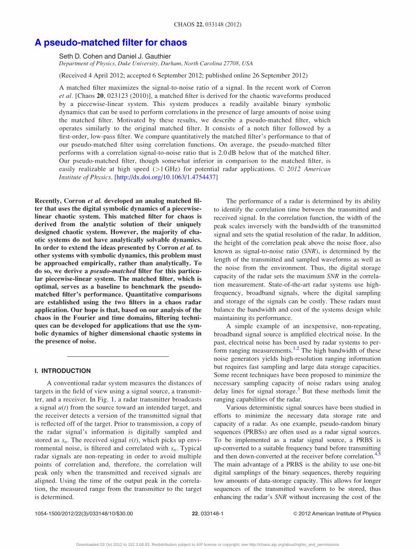
of nmðtÞ, y(t), and v(t), respectively. We plot the magnitudes
of Hinput, Ho, and Hm as a function of frequency � in Fig. 6.
In Fig. 6(d), we also plot the phase of Hm, where the phase is
approximately linear with frequency for � < 1 and thus pre-
serves timing information in sn.
We analyze Hinput and Ho individually to better under-
stand the matched filter’s transfer function. We factorize
Hinput into two linear operations (Hinput ¼ HnotchHintegrator), a
notch filter and an integrator
Hnotchð�Þ ¼~y
~q¼ e2pi� � 1; (9)
Hintegratorð�Þ ¼~q
~v¼ 1
2pi�; (10)
where ~q is the Fourier transform of an intermediate input-
output variable and Hnotch and Hintegrator are the transfer
functions of a notch filter and integrator, respectively. We
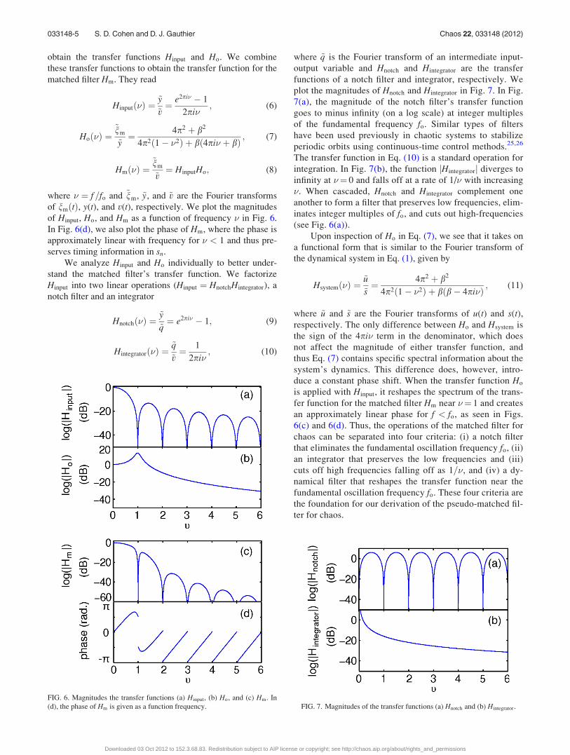
plot the magnitudes of Hnotch and Hintegrator in Fig. 7. In Fig.
7(a), the magnitude of the notch filter’s transfer function
goes to minus infinity (on a log scale) at integer multiples
of the fundamental frequency fo. Similar types of filters
have been used previously in chaotic systems to stabilize
periodic orbits using continuous-time control methods.25,26
The transfer function in Eq. (10) is a standard operation for
integration. In Fig. 7(b), the function jHintegratorj diverges to
infinity at �¼ 0 and falls off at a rate of 1/� with increasing
�. When cascaded, Hnotch and Hintegrator complement one
another to form a filter that preserves low frequencies, elim-
inates integer multiples of fo, and cuts out high-frequencies
(see Fig. 6(a)).
Upon inspection of Ho in Eq. (7), we see that it takes on
a functional form that is similar to the Fourier transform of
the dynamical system in Eq. (1), given by
Hsystemð�Þ ¼~u
~s¼ 4p2 þ b2
4p2ð1� �2Þ þ bðb� 4pi�Þ ; (11)
where ~u and ~s are the Fourier transforms of u(t) and s(t),respectively. The only difference between Ho and Hsystem is
the sign of the 4pi� term in the denominator, which does
not affect the magnitude of either transfer function, and
thus Eq. (7) contains specific spectral information about the
system’s dynamics. This difference does, however, intro-
duce a constant phase shift. When the transfer function Ho
is applied with Hinput, it reshapes the spectrum of the trans-
fer function for the matched filter Hm near �¼ 1 and creates
an approximately linear phase for f < fo, as seen in Figs.
6(c) and 6(d). Thus, the operations of the matched filter for
chaos can be separated into four criteria: (i) a notch filter
that eliminates the fundamental oscillation frequency fo, (ii)
an integrator that preserves the low frequencies and (iii)
cuts off high frequencies falling off as 1=�, and (iv) a dy-
namical filter that reshapes the transfer function near the
fundamental oscillation frequency fo. These four criteria are
the foundation for our derivation of the pseudo-matched fil-
ter for chaos.
FIG. 6. Magnitudes the transfer functions (a) Hinput, (b) Ho, and (c) Hm. In
(d), the phase of Hm is given as a function frequency. FIG. 7. Magnitudes of the transfer functions (a) Hnotch and (b) Hintegrator.
033148-5 S. D. Cohen and D. J. Gauthier Chaos 22, 033148 (2012)
Downloaded 03 Oct 2012 to 152.3.68.83. Redistribution subject to AIP license or copyright; see http://chaos.aip.org/about/rights_and_permissions

IV. PSEUDO-MATCHED FILTER
Our strategy for designing a pseudo-matched filter for
chaos is to simplify the four criteria of the matched filter
using transfer functions from components that are readily
available at high-speed. In Sec. V, we satisfy criteria (i) and
(ii) using a single transfer function. We also show that crite-
rion (iii) can be accomplished without an integrator. Lastly,
we demonstrate that criterion (iv) is not necessary for our
applications.
To begin constructing our pseudo-matched filter, we
select a different notch filter that is shifted in frequency but
still blocks the fundamental frequency fo. Most notch filters
block integer multiples (n¼ 0, 1, 2, 3,…) of a single fre-
quency. Instead, we choose a notch filter that is shifted to
block odd integer multiples (2nþ 1¼ 1, 3, 5,…) of a single
frequency. Since the matched filter attenuates frequencies
above �¼ 1, we conjecture that the only important spectral
notch is at fo, and all high-order even notches are not
included in our pseudo-matched filter. The transfer function
of our shifted-notch filter is
Hshifted�notchð�Þ ¼~vout
~vin¼ 1
2ð1þ epi�Þ; (12)
where ~vin and ~vout are the Fourier transforms of the input sig-
nal vin and output signal vout, respectively. We plot the mag-
nitude of Hshifted�notch in Fig. 8(a) (compare to Hnotch from
Fig. 7(a)). In both plots, the fundamental frequency fo is
blocked. However, in Fig. 8(a), the lower frequencies
(� < 0:5) are not cut. Thus, the shifted-notch filter performs
two of the four operations from the matched filter; (i) it elim-
inates the fundamental oscillation frequency fo and (ii) pre-
serves low frequencies.
In the time domain, the shifted-notch filter of Eq. (12) is
expressed by
voutðtÞ ¼1
2ðvinðtÞ þ vinðt� p=xoÞÞ: (13)
We compare Eq. (13) to Eq. (3) and note that the output is
no longer related to the input through a derivative. Also, the
time-shift on the input signal is halved (p=xo instead of
2p=xo) and the shifted input vinðt� p=xoÞ is summed with
the present state vinðtÞ. In an experimental setting using high-
speed electronics, where vin and vout are voltages, this
shifted-notch filter can be realized using a voltage divider,
time delays (realized, for example, by coaxial cables), and
an isolating hybrid junction, as illustrated in Fig. 9. The
lengths of the two cables used in this realization of the filter
are chosen such that the difference in propagation times
for electromagnetic waves to propagate through them is
sB � sA ¼ p=xo. The isolating hybrid junction sums the
outputs vðt� sAÞ þ vðt� sBÞ. We shift time t! tþ sA to
arrive at the output signal vout in Eq. (14). This realization
of the shifted-notch filter can scale to high-speed voltages
(>1 GHz).
Continuing the construction of the pseudo-matched fil-
ter, we use a first-order low-pass filter to attenuate high fre-
quencies, rather than an integrator. We avoid the need for an
integrator because the shifted-notch does not cut off low fre-
quencies. The transfer function of the low-pass (L-P) filter is
HL�Pð�Þ ¼~xout
~xin
¼ 1
1þ 2pi�=�L
; (14)
where xin and xout are the Fourier transforms of the input and
output signals, respectively, and the low-pass cutoff fre-
quency is �L ¼ fL=fo. We plot the magnitude of HL�P in Fig.
8(b). In the figure, HL�P leaves the spectral amplitude of fre-
quencies below �L unchanged, while suppressing frequencies
above �L. Beyond � ¼ �L, the rate of the spectral roll-off of
jHL�Pj is not ���1, but rather �ð1þ �Þ�1. A first-order low-
pass filter is a standard electronic component for filtering an
FIG. 8. Magnitudes of the transfer functions (a) Hshifted�notch, (b) HL�P, (c)
Hp. In (d), the phase of Hp is given as a function frequency.
FIG. 9. Pictorial realization for a high-speed (>1 GHz) shifted-notch filter
for voltages vin and vout. An example of a broadband, high-frequency power
splitter is the Mini-Circuits ZFRSC-42-S, and an example of a broadband,
high-frequency hybrid-junction is the M/A-COM H-9.
033148-6 S. D. Cohen and D. J. Gauthier Chaos 22, 033148 (2012)
Downloaded 03 Oct 2012 to 152.3.68.83. Redistribution subject to AIP license or copyright; see http://chaos.aip.org/about/rights_and_permissions

input voltage xin to obtain an output voltage xout and satisfies
approximately the third component of the matched filter cri-
teria (iii). We note that higher-order low-pass filters (Butter-
worth, Chebyshev, etc.) are also available at high-speed.
When constructing our pseudo-matched filter, we neglect
the dynamical filter that reshapes the spectrum (iv). We show
that using just the shifted-notch and low-pass filters allows us
to achieve comparable performance to the true matched filter
in a simulated radar application. Thus, we cascade the shifted-
notch and low-pass filters (Hshifted�notchHL�P) to arrive at the
transfer function of our pseudo-matched filter
Hpð�Þ ¼~vout
~vin¼ 1þ epi�
2þ 4pi�=�L; (15)
where ~vin and ~vout are the Fourier transforms of the input and
output signals of the filter, respectively. We plot the magni-
tude and phase of Hp in Fig. 8(c). In the figure, the phase of
Hp is approximately linear and thus preserves timing infor-
mation from v(t). For comparison to the matched filter, see
Fig. 6(c). Qualitatively, the two filters follow similar trends
in both magnitude and phase. The phase in the pseudo-
matched filter has a lower slope in its frequency dependence;
a lower slope just constitutes a shorter time delay through
the filter. However, it is clear by comparison of the magni-
tudes that the pseudo-matched filter is not performing the
same operations as the matched filter.
We now apply the pseudo-matched filter to the chaotic
waveform generated by Eqs. (1) and (2) and examine its out-
put in the time-domain. We drive the pseudo-matched filter
with v(t)¼ u(t)þAWGN, where v(t) has a SNR of �5.9 dB
(see Fig. 3(c)). In Fig. 10(a), we plot the pseudo-matched fil-
ter’s output npðtÞ. From the figure, we see that pseudo-
matched filter has effectively removed the main oscillation
frequency fo and what remains is a digital-like signal npðtÞ.We note that a considerable amount of noise is still present
in comparison to Fig. 3(d). Using a correlation between the
original s(t) and npðtÞ, we determine the time delay through
the pseudo-matched filter sp to be approximately 0:14=fo.
We compensate for the delay, and sample npðtÞ at fo, assign-
ing binary values using the relation: �1 if npðtnÞ � 0 and þ1
if npðtnÞ > 0, where tn is the nth sampling time. In Fig.
10(a), we see that, with this particular SNR, the discrete sam-
pling of npðtÞ is equivalent to sn from Fig. 3(b).
Next, we parallel the construction of the time delay tap
from Eq. (5) for the output of the pseudo-matched filter. In
this case, the time delay tap is
vpðtÞ ¼XN
n¼1
snnpðt� tnÞ; (16)
where vpðtÞ is the output of the time-domain correlation. We
plot an example of vpðtÞ in Fig. 10(b) using the same chaos
and sn that were used to calculate vmðtÞ in Fig. 4. By visually
comparing vpðtÞ to vmðtÞ, we see that the output correlation
peaks are qualitatively similar, but vpðtÞ has more noise. In
the remaining section, we establish criteria for quantitatively
comparing these correlation waveforms and use these criteria
to weigh each filter’s performance.
V. MATCHED VS. PSEUDO-MATCHED
In order to quantitatively compare the performances of
the matched and pseudo-matched filters, we examine each
filter’s ability to recover sequences of the system’s symbolic
dynamics within the context of a chaos radar. In all radar
applications, the ability to correctly identify the location of
the correlation peak in the correlation operation is the useful
measure. Therefore, in order to compare the two filters, we
examine their performances based on the peak width and
output SNR of vm;pðtÞ. We also present an approximate ana-
lytical form for each correlation’s output SNR.
The peak widths of the output-correlation functions give
the resolutions of each radar system. We measure Dm and
Dp, the full-width at half maximum (FWHM) time of the cor-
relation output peaks using the matched and pseudo-matched
filters, respectively. For the most ideal measure of each fil-
ter’s correlation peak width, we measure Dm;p in cases where
no noise is present in the received waveform v(t)¼ u(t). We
note that these widths are independent of N, the number of
stored data points in the correlation calculation of Eqs. (5)
and (16). Using a Gaussian fit to the peak of vm;pðtÞ, we
obtain peak widths Dmfo ¼ 0:55 and Dpfo ¼ 0:73 (see Ap-
pendix). Using these values of Dm;p and scaling fo to 1 GHz,
we calculate the theoretical resolutions of the matched and
pseudo-matched filters to be 0.17 m and 0.22 m, respectively.
In this example, the ranging resolutions differ by 5 cm. Thus,
this is not a critical difference for radar applications that
localize targets like planes or cars, and the pseudo-matched
filter has an acceptable ranging resolution in comparison to
the matched filter.
Next, we measure the output correlation SNR’s of the
matched and pseudo-matched filters using the correlation
FIG. 10. Output of pseudo-matched filter. (a) Time series of the output of
the matched filter npðtÞ (blue) while driven by v(t)¼ u(t)þAWGN(SNR¼�5.9 dB). The signal npðtÞ is sampled with uniform spacing (red
dots) at a clock frequency fo ¼ xo=2p. Above the waveform, a single-bit
discrete sampling of the waveform is shown. From the figure, we see that all
of the relevant information from sn is encoded in npðtÞ. (b) The switching
state s(t) is sampled and sn is stored for N¼ 100. The output of the pseudo-
matched filter npðtÞ drives Eq. (16) and the output vpðtÞ peaks at time
t ¼ 2spd þ sp.
033148-7 S. D. Cohen and D. J. Gauthier Chaos 22, 033148 (2012)
Downloaded 03 Oct 2012 to 152.3.68.83. Redistribution subject to AIP license or copyright; see http://chaos.aip.org/about/rights_and_permissions

peak heights am;p and the surrounding correlation noise
floors. The output SNR in vm;pðtÞ is
SNRm;p ¼a2
m;p
r2Njm;p
; (17)
where am;p is the peak height of nm;pðtÞ from a Gaussian fit
(see Appendix) and r2Njm;p is the output variance of the corre-
lation noise floor (note that the mean of the noise floor �0)
for the matched and pseudo-matched filters, respectively.
We present a summary of these quantities in the block
diagram shown in Fig. 11(a). In the diagram, we also review
the waveforms and processes used for generating nm;pðtÞ and
vm;pðtÞ and highlight the two relevant quantities, SNRinput
and SNRm;p. We calculate SNRm;p as a function of the input
SNRinput. The results of these calculations are given in
Fig. 11(b). In addition, we use the distributions from nmðtÞand npðtÞ from the two different cases v(t)¼AWGN and
v(t)¼ u(t) to derive an analytical prediction for SNRm;p (see
Appendix for derivations). These theoretical predictions are
plotted with dotted lines in Fig. 11(b). These plots represent
the performances of the matched and pseudo-matched filters
in a simulated radar.
From Fig. 11(b), it is clear that the matched filter
outperforms the pseudo-matched filter in the output SNR of a
radar correlation. Without noise in the system, the matched
and pseudo-matched filters perform with output correlation
SNR’s of 2:6þ 10log10ðNÞ dB and 1:3þ 10log10ðNÞ dB,
respectively. For SNRinput ¼ 1=100, the output SNR’s
decrease to �2:0þ 10log10ðNÞ dB and �44þ 10log10ðNÞdB, respectively. In Fig. 11(b), the average difference
between SNRm and SNRp is 2.0 dB. We note that this differ-
ence is independent of N and therefore fully characterizes
the filter performances. Thus, where small loss is acceptable
in the performance of the radar, the pseudo-matched filter is
a simpler alternative to the system’s analytically matched fil-
ter for chaos.
As a final example, we use the theoretical SNRm;p to pre-
dict when the matched and pseudo-matched filters will fail in
a radar application. Failure occurs when SNRm;p falls below
a certain threshold. For a radar system that is capable of
storing N¼ 50 data points and has a desired output correla-
tion SNR of 33 dB, the matched and pseudo-matched filters
will fail at a 1=SNRinput of approximately 25 and 70, respec-
tively. If, in this application, the input SNR is such that
1=SNRintput < 10, then a radar with either the matched or
pseudo-matched filter will be able to range, on average, with-
out failure. The choice between the matched and pseudo-
matched filter is therefore an application-dependent problem,
and, as the bandwidth of this system scales higher, one must
also begin to weigh each filter’s high-frequency capabilities
as well as its baseline performance.
VI. CONCLUSIONS
In conclusion, for the chaotic system presented in Ref.
18, we derive empirically a sub-optimal filter for increasing
the SNR of a chaotic waveform. This sub-optimal filter per-
forms approximately three out of four of the linear opera-
tions from the matched filter for chaos: (i) eliminates the
fundamental oscillation frequency fo, (ii) preserves the low
frequencies, and (iii) cuts off high frequencies. Our filter,
deemed a pseudo-matched filter, is composed of a shifted-
notch filter and a first-order low-pass filter. In the context of
a radar concept that uses a time delay tap as a correlation
measure, we have shown that the pseudo-matched filter may
be an acceptable and simplified substitute for the matched fil-
ter. In addition, we acknowledge that the psuedo-matched fil-
ter can be further improved using higher order low-pass
filters and additional shifted-notch filters. We present this
current version of the pseudo-matched filter to illustrate our
method and emphasize its simplicity.
We note that our analysis highlights the flexibility and
robustness of Corron et al.’s findings. The chaos from the dy-
namical system in Eqs. (1) and (2), even in the presence of
large amounts of noise, can be processed by a linear filter to
perform correlations with its symbolic dynamics. We capital-
ize on this system’s elegance to create a simpler, so-called
pseudo-matched filter. Although sub-optimal, the pseudo-
matched filter shows that the advantages of this chaotic sys-
tem can be adapted for applied settings that use commercially
available, high-speed filters. In the future, in order to make
use of this specific high-speed, pseudo-matched filter, we
acknowledge that a high-frequency version of this dynamical
system must also be constructed. But, it is our hope that, in
FIG. 11. (a) Block diagram for testing the matched and pseudo-matched fil-
ters in a simulated radar application. (b) Output-correlation SNR’s of the
matched (blue w) and pseudo-matched (red�) filters scaled by N on a log-
arithmic scale as a function of 1=SNRinput. For each value of SNRinput, 100
calculations of SNRm;p were performed using sequence of sn for n ¼ no to
n ¼ no þ N, where no is a random positive integer and N¼ 50. The mean
value of the calculated SNRm;p is plotted with the respective standard devia-
tions. The blue and red dotted lines give the theoretical predictions of the
SNRm;p as references for the matched and pseudo-matched filters, respec-
tively. Cases for larger N were verified to have quantitatively similar results.
033148-8 S. D. Cohen and D. J. Gauthier Chaos 22, 033148 (2012)
Downloaded 03 Oct 2012 to 152.3.68.83. Redistribution subject to AIP license or copyright; see http://chaos.aip.org/about/rights_and_permissions

the meantime, this work inspires others to investigate deeper
into the symbolic dynamics of all chaotic systems and find
applications that benefit from an empirically derived pseudo-
matched filter for chaos (LADAR, communications, etc.).
ACKNOWLEDGMENTS
We gratefully acknowledge Damien Rontani for useful
discussions, G. Martin Hall with help in radar concepts, and
the financial support of Propagation Research Associates
(PRA) Grant No. W31P4Q-11-C-0279.
APPENDIX A: ADDITIVE NOISE
Because the output from MATLAB’s ODE45 uses a vari-
able timestep, we resample u(t) using a linear interpolation
with time steps dt, where dtfo ¼ 10�2. To simulate environ-
mental noise, we add noise to the waveform u(t) using ran-
dom numbers spaced by time units dt. The random numbers
are calculated from a Gaussian distribution with zero mean.
For different points along the 1=SNRinput axis of Fig. 11(b),
the variance of the AWGN is varied accordingly.
APPENDIX B: GAUSSIAN FITS
We measure the correlation peak width and height using
a Gaussian fit
f ðtÞ ¼ am;peðt�ð2spdþsm;pÞÞ2=2c2m;p ; (B1)
where am;p and cm;p are free parameters that are fit to the cor-
relation peak heights and widths. Using f ðtÞ to fit vm;pðtÞ, we
obtain a FWHM peak width Dm;pfo ¼ 2ffiffiffiffiffiffiffiffiffiffiffiffiffi2lnð2Þ
pcm;p and
peak height am;p.
APPENDIX C: ANALYTICAL SNR’S
We derive analytical forms for the output-correlation
SNR of the matched and pseudo-matched filters. To do so,
we approximate Eq. (17) as
SNRm;p ¼a2
m;p
r2Njm;p
� ðAm;pNÞ2
r21jm;pN þ r2
2jm;pN; (C1)
where Am;p is a constant that characterizes the growth
rate of the correlation peak height with N, r21jm;p is a
constant determined in the noise-free case where v(t)¼ u(t),and r2
2jm;p is a function of SNRinput in the case where
v(t)¼AWGN. Recall that the numerators and denominators
of Eq. (C1) represent the power of peak heights of the cor-
relation and the surrounding noise floor, respectively. We
derive each of the three terms Am;p, r21jm;p, and r2
2jm;p in the
following sections.
The correlation peak heights for the matched and
pseudo-matched filters grow at different rates. In the correla-
tion operations of Eqs. (5) and (16), the peaks occur at times
t�m;p ¼ 2spd þ sm;p for the matched and pseudo-matched fil-
ters, respectively. At time t�m;p, nm;pðtÞ is aligned with sn and
the output correlation is
vm;pðt�m;pÞ �XN
n¼1
jnm;pðt�m;p � tnÞj � Am;pN: (C2)
We approximate Am;p from the local maxima of jnm;pðtÞj. To
do so, we examine the noise-free case where v(t)¼ u(t) and
collect a subset of points jnm;pðtðrÞm;pÞj, where tðrÞm;p are the times
of local maxima in jnm;pðtÞj. We average jnm;pðtðrÞm;pÞj to
obtain Am ¼ 1:34 and Ap ¼ 1:02 using a time-length
tfo � 104.
To approximate the value of r21jm;p, we also examine
nm;pðtÞ in the noise-free case where v(t)¼ u(t). The determinis-
tic noise floor in a correlation measurement is also known as
its side-lobes; the side-lobes result from non-zero contributing
terms in the correlation vm;pðtÞ when t 6¼ t�m;p. Using the
central limit theorem, we approximate the variance of these
nonzero terms as r21jm;pN, where r2
1jm;p is the variance of the
signal nm;pðtÞ. In this approximation, we find that r21jm ¼ 1:00
and r21jp ¼ 0:78.
It remains to calculate the contributions to the noise
floor of the correlation from additive noise. To do so, we
examine nm;pðtÞ in the case where v(t)¼AWGN. Similar to
the case for the side-lobes, we use the central limit theorem
to approximate the contribution of the AWGN to the noise
floor of the correlation as r22jm;pN, where r2
2jm;p is the var-
iance of the signal nm;pðtÞ. However, r22jm;p depends on the
variance of the input AWGN
r22jm;p ¼ am;pr
2AWGN; (C3)
where am;p is the noise attenuation factor of the matched and
pseudo-matched filters, respectively. We measure the values
am ¼ 1=75 and ap ¼ 1=64. Lastly, we use that r2AWGN ¼
r2u=ðSNRinputÞ to rewrite Eq. (C1) as
SNRm;p � NA2
m;p
r21jm;p þ am;p
r2u
SNRinput
; (C4)
where r2u ¼ 1:34 is the power of the chaotic signal u(t). We
plot Eq. (C4) as a function of 1=SNRinput for the matched and
pseudo-matched filters in Fig. 11(b).
1G. S. Liu, H. Gu, W. M. Su, H. B. Sun, and J. H. Zhang, IEEE Trans.
Aerosp. Electron. Syst. 39, 489 (2003).2D. Tarchi, K. Lukin, J. Fortuny-Guasch, A. Mogyla, P. Vyplavin, and A.
Sieber, IEEE Trans Aerosp. Electron. Syst. 46, 1214 (2010).3K. Lukin, P. Vyplavin, O. Zemlyaniy, S. Lukin, and V. Palamarchuk,
Proc. SPIE 8021, 802114 (2011).4I. Urazghildiiev, R. Ragnarsson, P. Ridderstrom, A. Rydberg, E. Ojefors,
K. Wallin, P. Enochsson, M. Ericson, and G. Lofqvist, IEEE Trans. Intell.
Transp. Syst. 8, 245 (2007).5M. Mirshafiei, A. Ghazisaeidi, D. Lemus, S. LaRochelle, and L. A. Rusch,
J. Lightwave Technol. 30, 207 (2012).6A. Dmitriev, E. Efremova, L. Kuzmin, and N. Atanov, Int. J. Bifurcation
Chaos Appl. Sci. Eng. 17, 3443 (2007).7M. H. Khan, H. Shen, Y. Xuan, L. Zhao, S. Xiao, D. E. Leaird, A. M.
Weiner, and M. Qi, Nature Photon. 4, 117 (2010).8M. I. Sobhy and A. Shehata, IEEE MTT-S Int. Microwave Symp. Dig. 3,
1701 (2000).9Y. C. Kouomou, P. Colet, L. Larger, and N. Gastaud, Phys. Rev. Lett. 95,
203903 (2005).10L. Illing and D. J. Gauthier, Chaos 16, 033119 (2006).
033148-9 S. D. Cohen and D. J. Gauthier Chaos 22, 033148 (2012)
Downloaded 03 Oct 2012 to 152.3.68.83. Redistribution subject to AIP license or copyright; see http://chaos.aip.org/about/rights_and_permissions

11R. Zhang, H. L. D. S. Cavalcante, Z. Gao, D. J. Gauthier, J. E. S. Socolar,
M. M. Adams, and D. P. Lathrop, Phys. Rev. E 80, 045202(R) (2009).12K. M. Myneni, T. A. Barr, B. R. Reed, S. D. Pethel, and N. J. Corron,
Appl. Phys. Lett. 78, 1496 (2001).13F. Lin and L. Jia-Ming, IEEE J. Quantum Electron. 40, 682 (2004).14V. Venkatasubramanian and H. Leung, IEEE Signal Process. Lett. 12, 528
(2005).15V. Venkatasubramanian and H. Leung, IEEE Trans. Image Process. 18,
1255 (2009).16S.-L. Chen, T. Hwang, S.-M. Chang, and W.-W. Lin, Int. J. Bifurcation
Chaos Appl. Sci. Eng. 20, 3969 (2010).17T. Saito, Electron. Commun. Jpn. Pt. I 64, 9 (1981).18N. J. Corron, J. N. Blakely, and M. T. Stahl, Chaos 20, 023123 (2010).
19J. N. Blakely and N. J. Corron, Proc. SPIE 8021, 80211H (2010).20J. G. Proakis, Digital Communications, 4th ed. (McGraw-Hill, 2001),
Chap. 5, p. 231.21A. Tamasevicius, G. Mykolaitis, S. Bumeliene, A. Baziliauskas, R. Kri-
vickas, and E. Lindberg, Nonlinear Dyn. 46, 159 (2006).22Y. I. Ismail and E. G. Friedman, IEEE Trans. Very Large Scale Integr.
(VLSI) Syst. 8, 195 (2000).23P. Withington, H. Fluhler, and S. Nag, IEEE Microw. Mag. 4, 51 (2003).24A. R. Volkovskii, L. S. Tsimring, N. F. Rulkov, and I. Langmore, Chaos
15, 033101 (2005).25K. Pyragas, Phys. Lett. A 170, 421 (1992).26J. E. S. Socolar, D. W. Sukow, and D. J. Gauthier, Phys. Rev. E 50,
3245–3248 (1994).
033148-10 S. D. Cohen and D. J. Gauthier Chaos 22, 033148 (2012)
Downloaded 03 Oct 2012 to 152.3.68.83. Redistribution subject to AIP license or copyright; see http://chaos.aip.org/about/rights_and_permissions