Ad

RB

a

ARRA

KCPPPU

1

saioniawlcddsaumaao

0h

Energy and Buildings 55 (2012) 481–493

Contents lists available at SciVerse ScienceDirect

Energy and Buildings

j ourna l ho me p age: www.elsev ier .com/ locate /enbui ld

proposed method for generating high resolution current and future climateata for Passivhaus design

obert S. McLeod ∗, Christina J. Hopfe, Yacine RezguiRE Institute of Sustainable Engineering, Cardiff University, CF24 3AA, Wales, UK

r t i c l e i n f o

rticle history:eceived 17 May 2012eceived in revised form 6 August 2012ccepted 28 August 2012

eywords:limate change scenariosrobabilistic climate data

a b s t r a c t

The sensitivity of low energy and passive solar buildings to their climatic context creates a requirementfor accurate local climate data. This situation takes on increasing importance in the context of modellingPassivhaus buildings where the absence of conventional oversized heating and cooling systems implies agreater reliance upon fabric and system optimisation. Conversely, future climatic changes may also poseserious implications for super insulated buildings with inadequate solar shading. Currently, many widelyused building performance simulation (BPS) tools still rely on very limited sources of climate data.

The following research examines the need for regional and, in some cases, micro-regional climatic data

assivhausHPPrban heat islands

when designing ultra-low energy Passivhaus buildings in the UK. The paper proposes a new methodologyfor generating this data in PHPP format. The data generated is compared to alternative sources, and theimplications discussed in the context of three case studies examining a certified Passivhaus dwelling ina mountainous region of Wales as well as two locations, in close proximity, within London. If correctlyimplemented the use of such data should provide a more robust basis for future cost and performanceoptimisation in low energy and passive building design.

. Introduction

Passivhaus Planning Package (PHPP12) is a simplified steadytate building simulation tool that is primarily targeted at assistingrchitects and mechanical engineers in designing Passivhaus build-ngs [1]. According to the Passivhaus Institute (PHI) the verificationf a Passivhaus design must be carried using the Passivhaus Plan-ing Package (PHPP). As a result, this quasi-steady state software

s the de facto software used for both the design and compli-nce predictions of Passivhaus buildings in the UK and around theorld. PHPP has been validated using both dynamic thermal simu-

ations using Dynbil [2] and empirical data from a large number ofompleted Passivhaus projects [3]. Dynamic simulation results pre-icted by Dynbil, have also been extensively compared to measuredata for both dwellings and office buildings [4–6]. PHPP validationtudies have generally shown good agreement between measurednd predicted results including those derived from dynamic sim-lation [3]. The PHPP thermal model conforms to the calculationethods set out in EN ISO 13790 for determining heating demand

ccording to annual or monthly methods, and contains additionallgorithms to calculate peak heating and cooling loads and assessverheating risks.

∗ Corresponding author. Tel.: +44 29 208 70368.E-mail address: McLeodRS@cardiff.ac.uk (R.S. McLeod).

378-7788/$ – see front matter © 2012 Elsevier B.V. All rights reserved.ttp://dx.doi.org/10.1016/j.enbuild.2012.08.045

© 2012 Elsevier B.V. All rights reserved.

In addition to delivering design energy and peak load predic-tions a validated PHPP worksheet is primarily used to demonstratecompliance with the Passivhaus certification criteria. The key crite-ria for Passivhaus certification are that the building must havea specific annual heat demand (qH) ≤ 15 kWh/m2 yr or a specificpeak load (pH) ≤ 10 W/m2, together with a specific primary energydemand (qp) ≤ 120 kWh/m2 yr relative to the treated floor area(TFA). Where a cooling energy requirement exists this must alsobe (qc) ≤ 15 kWh/m2 yr.

Like all building physics models the outputs from the PHPPmodel are predicated upon the use of appropriate boundary con-ditions. In the case of PHPP where, for certification purposes, theinternal gains (residential, 2.1 W/m2) and operative temperature(20 ◦C) are assumed to remain constant; the key boundary con-ditions used to determine the annual heating demand, coolingdemand and peak loads depend almost entirely on the externalclimate.

In the context of a Passivhaus, where all of the supplementaryheating may be provided solely via a small post-air heater, the riskassociated with uncertainty in the peak heating load calculationscould have real consequences. Conversely, overheating risks arelikely to increase with climate change and a better understanding

of cooling loads and future overheating risk predictions is needed[7]. Hence, there is a need to understand the uncertainty associatedwith the climate files used in order to determine the sensitivityand reliability of any design or certification predictions. Typical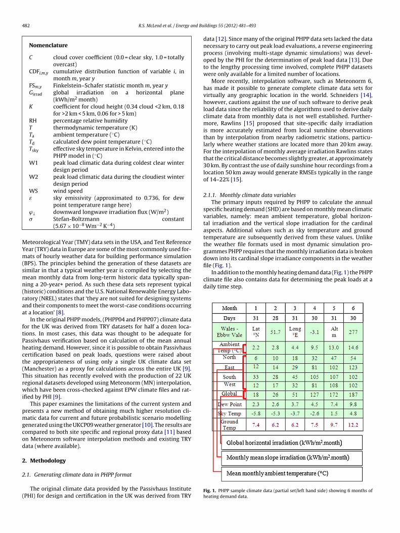

482 R.S. McLeod et al. / Energy and Bu

Nomenclature

C cloud cover coefficient (0.0 = clear sky, 1.0 = totallyovercast)

CDFi,m,y cumulative distribution function of variable i, inmonth m, year y

FSm,y Finkelstein–Schafer statistic month m, year yGirrad global irradiation on a horizontal plane

(kWh/m2 month)K coefficient for cloud height (0.34 cloud <2 km, 0.18

for >2 km < 5 km, 0.06 for > 5 km)RH percentage relative humidityT thermodynamic temperature (K)Ta ambient temperature (◦C)Td calculated dew point temperature (◦C)Tsky effective sky temperature in Kelvin, entered into the

PHPP model in (◦C)W1 peak load climatic data during coldest clear winter

design periodW2 peak load climatic data during the cloudiest winter

design periodWS wind speedε sky emissivity (approximated to 0.736, for dew

point temperature range here)ϕ downward longwave irradiation flux (W/m2)

MYm(smn(raa

ftPhct(Trwi

pmgcod

2

2

(

file (Fig. 1).In addition to the monthly heating demand data (Fig. 1) the PHPP

climate file also contains data for determining the peak loads at adaily time step.

↓� Stefan-Boltzmann constant

(5.67 × 10−8 Wm−2 K−4)

eteorological Year (TMY) data sets in the USA, and Test Referenceear (TRY) data in Europe are some of the most commonly used for-ats of hourly weather data for building performance simulation

BPS). The principles behind the generation of these datasets areimilar in that a typical weather year is compiled by selecting theean monthly data from long-term historic data typically span-

ing a 20-year+ period. As such these data sets represent typicalhistoric) conditions and the U.S. National Renewable Energy Labo-atory (NREL) states that ‘they are not suited for designing systemsnd their components to meet the worst-case conditions occurringt a location’ [8].

In the original PHPP models, (PHPP04 and PHPP07) climate dataor the UK was derived from TRY datasets for half a dozen loca-ions. In most cases, this data was thought to be adequate forassivhaus verification based on calculation of the mean annualeating demand. However, since it is possible to obtain Passivhausertification based on peak loads, questions were raised abouthe appropriateness of using only a single UK climate data setManchester) as a proxy for calculations across the entire UK [9].his situation has recently evolved with the production of 22 UKegional datasets developed using Meteonorm (MN) interpolation,hich have been cross-checked against EPW climate files and rat-

fied by PHI [9].This paper examines the limitations of the current system and

resents a new method of obtaining much higher resolution cli-atic data for current and future probabilistic scenario modelling

enerated using the UKCP09 weather generator [10]. The results areompared to both site specific and regional proxy data [11] basedn Meteonorm software interpolation methods and existing TRYata (where available).

. Methodology

.1. Generating climate data in PHPP format

The original climate data provided by the Passivhaus InstitutePHI) for design and certification in the UK was derived from TRY

ildings 55 (2012) 481–493

data [12]. Since many of the original PHPP data sets lacked the datanecessary to carry out peak load evaluations, a reverse engineeringprocess (involving multi-stage dynamic simulations) was devel-oped by the PHI for the determination of peak load data [13]. Dueto the lengthy processing time involved, complete PHPP datasetswere only available for a limited number of locations.

More recently, interpolation software, such as Meteonorm 6,has made it possible to generate complete climate data sets forvirtually any geographic location in the world. Schneiders [14],however, cautions against the use of such software to derive peakload data since the reliability of the algorithms used to derive dailyclimate data from monthly data is not well established. Further-more, Rawlins [15] proposed that site-specific daily irradiationis more accurately estimated from local sunshine observationsthan by interpolation from nearby radiometric stations, particu-larly where weather stations are located more than 20 km away.For the interpolation of monthly average irradiation Rawlins statesthat the critical distance becomes slightly greater, at approximately30 km. By contrast the use of daily sunshine hour recordings from alocation 50 km away would generate RMSEs typically in the rangeof 14–22% [15].

2.1.1. Monthly climate data variablesThe primary inputs required by PHPP to calculate the annual

specific heating demand (SHD) are based on monthly mean climaticvariables, namely: mean ambient temperature, global horizon-tal irradiation and the vertical slope irradiation for the cardinalaspects. Additional values such as sky temperature and groundtemperature are subsequently derived from these values. Unlikethe weather file formats used in most dynamic simulation pro-grammes PHPP requires that the monthly irradiation data is brokendown into its cardinal slope irradiance components in the weather

Fig. 1. PHPP sample climate data (partial set/left hand side) showing 6 months ofheating demand data.

R.S. McLeod et al. / Energy and Bu

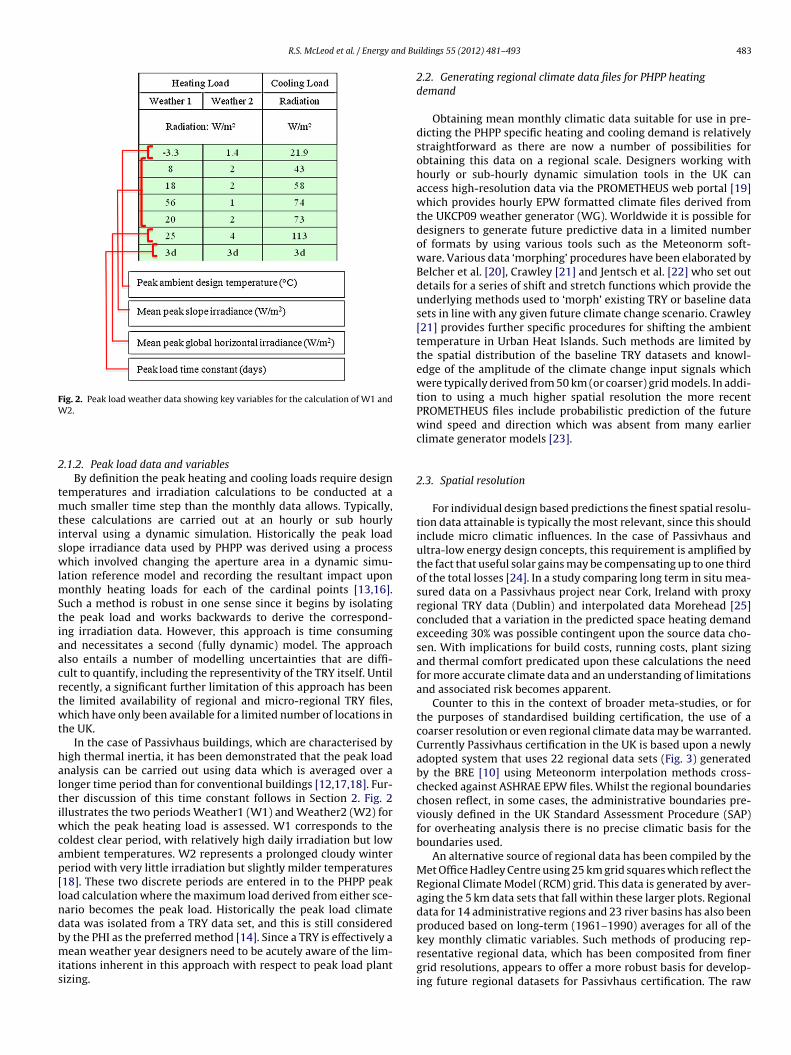
Fig. 2. Peak load weather data showing key variables for the calculation of W1 andW

2

tmtiswlmStiaacrtwt

haltiwcap[lndbmis

key monthly climatic variables. Such methods of producing rep-resentative regional data, which has been composited from finer

2.

.1.2. Peak load data and variablesBy definition the peak heating and cooling loads require design

emperatures and irradiation calculations to be conducted at auch smaller time step than the monthly data allows. Typically,

hese calculations are carried out at an hourly or sub hourlynterval using a dynamic simulation. Historically the peak loadlope irradiance data used by PHPP was derived using a processhich involved changing the aperture area in a dynamic simu-

ation reference model and recording the resultant impact upononthly heating loads for each of the cardinal points [13,16].

uch a method is robust in one sense since it begins by isolatinghe peak load and works backwards to derive the correspond-ng irradiation data. However, this approach is time consumingnd necessitates a second (fully dynamic) model. The approachlso entails a number of modelling uncertainties that are diffi-ult to quantify, including the representivity of the TRY itself. Untilecently, a significant further limitation of this approach has beenhe limited availability of regional and micro-regional TRY files,hich have only been available for a limited number of locations in

he UK.In the case of Passivhaus buildings, which are characterised by

igh thermal inertia, it has been demonstrated that the peak loadnalysis can be carried out using data which is averaged over aonger time period than for conventional buildings [12,17,18]. Fur-her discussion of this time constant follows in Section 2. Fig. 2llustrates the two periods Weather1 (W1) and Weather2 (W2) for

hich the peak heating load is assessed. W1 corresponds to theoldest clear period, with relatively high daily irradiation but lowmbient temperatures. W2 represents a prolonged cloudy wintereriod with very little irradiation but slightly milder temperatures18]. These two discrete periods are entered in to the PHPP peakoad calculation where the maximum load derived from either sce-ario becomes the peak load. Historically the peak load climateata was isolated from a TRY data set, and this is still consideredy the PHI as the preferred method [14]. Since a TRY is effectively aean weather year designers need to be acutely aware of the lim-

tations inherent in this approach with respect to peak load plantizing.

ildings 55 (2012) 481–493 483

2.2. Generating regional climate data files for PHPP heatingdemand

Obtaining mean monthly climatic data suitable for use in pre-dicting the PHPP specific heating and cooling demand is relativelystraightforward as there are now a number of possibilities forobtaining this data on a regional scale. Designers working withhourly or sub-hourly dynamic simulation tools in the UK canaccess high-resolution data via the PROMETHEUS web portal [19]which provides hourly EPW formatted climate files derived fromthe UKCP09 weather generator (WG). Worldwide it is possible fordesigners to generate future predictive data in a limited numberof formats by using various tools such as the Meteonorm soft-ware. Various data ‘morphing’ procedures have been elaborated byBelcher et al. [20], Crawley [21] and Jentsch et al. [22] who set outdetails for a series of shift and stretch functions which provide theunderlying methods used to ‘morph’ existing TRY or baseline datasets in line with any given future climate change scenario. Crawley[21] provides further specific procedures for shifting the ambienttemperature in Urban Heat Islands. Such methods are limited bythe spatial distribution of the baseline TRY datasets and knowl-edge of the amplitude of the climate change input signals whichwere typically derived from 50 km (or coarser) grid models. In addi-tion to using a much higher spatial resolution the more recentPROMETHEUS files include probabilistic prediction of the futurewind speed and direction which was absent from many earlierclimate generator models [23].

2.3. Spatial resolution

For individual design based predictions the finest spatial resolu-tion data attainable is typically the most relevant, since this shouldinclude micro climatic influences. In the case of Passivhaus andultra-low energy design concepts, this requirement is amplified bythe fact that useful solar gains may be compensating up to one thirdof the total losses [24]. In a study comparing long term in situ mea-sured data on a Passivhaus project near Cork, Ireland with proxyregional TRY data (Dublin) and interpolated data Morehead [25]concluded that a variation in the predicted space heating demandexceeding 30% was possible contingent upon the source data cho-sen. With implications for build costs, running costs, plant sizingand thermal comfort predicated upon these calculations the needfor more accurate climate data and an understanding of limitationsand associated risk becomes apparent.

Counter to this in the context of broader meta-studies, or forthe purposes of standardised building certification, the use of acoarser resolution or even regional climate data may be warranted.Currently Passivhaus certification in the UK is based upon a newlyadopted system that uses 22 regional data sets (Fig. 3) generatedby the BRE [10] using Meteonorm interpolation methods cross-checked against ASHRAE EPW files. Whilst the regional boundarieschosen reflect, in some cases, the administrative boundaries pre-viously defined in the UK Standard Assessment Procedure (SAP)for overheating analysis there is no precise climatic basis for theboundaries used.

An alternative source of regional data has been compiled by theMet Office Hadley Centre using 25 km grid squares which reflect theRegional Climate Model (RCM) grid. This data is generated by aver-aging the 5 km data sets that fall within these larger plots. Regionaldata for 14 administrative regions and 23 river basins has also beenproduced based on long-term (1961–1990) averages for all of the

grid resolutions, appears to offer a more robust basis for develop-ing future regional datasets for Passivhaus certification. The raw

484 R.S. McLeod et al. / Energy and Buildings 55 (2012) 481–493

used

df

2

tCvtgoodt

woB2

Fig. 3. 22 UK climatic regions currently

ata produced by the UKCP09 WG is not directly available in PHPPormat however.

.4. UKCP09 probabilistic data and weather generator

The HadRM3 RCM was developed by the Met Office Hadley Cen-re in order to downscale the simulations provided by the Globallimate Model (GCM). The RCM operates at a 25 km resolution, pro-iding outputs on a scale that is useful for impact assessment inhe built environment. This model creates 434 unique land basedrid squares containing probabilistic climate projections for mostf the UK. For each 25 km grid location 10,000 realisations (samplesf the probability density function) have been generated for eachecade and emissions scenario based on equi-probable changes inhe underlying climatic variables.

The weather generator is a climate model downscaling tool

hich was developed by the Hadley Centre in order to provide

utputs at a higher resolution than the regional climate model.y mapping the unique climate signal contained within each5 km grid square on to a much finer 5 km grid baseline (Fig. 4)

for Passivhaus certification (BRE, 2011).

approximately 11,000 viable grid data locations are produced cov-ering the entire UK landmass. Each 5 km grid square thus containsa 30 year baseline dataset for the reference period 1961–1990, cou-pled with the possibility to sample future probabilistic scenarios at10-year intervals from 2020 to 2080 [26].

Three climate change scenario outputs are available from theWeather Generator based on the Intergovernmental Panel on Cli-mate Change (IPCC) Special Report on Emissions Scenarios (SRES)climate principal scenarios: High (A1F1), medium (A1B) and low(B1). Further information on the global economic scenarios defin-ing the SRES scenarios can be found in IPCC [27]. Each WG runrandomly samples from the 10,000 change factors available to cre-ate a continuous thirty year time series based on the underlyingbaseline profile. A minimum of 100 randomly chosen samples ofthe WG climate data are needed to compile a single statisticallyrepresentative climate file. Each WG run therefore results in a min-

imum of 3000 equi-probable future weather years of data. The WGoperates at a daily temporal scale from which hourly variables aresubsequently extrapolated based on existing relationship patternsin the observed baseline data.

R.S. McLeod et al. / Energy and Buildings 55 (2012) 481–493 485

grid re

uAdomsfsMn[ds

tdeitd

2

biutcd

2oi

G

waN

fb

Fig. 4. Showing UKCP09 5 km and 25 km

Rainfall is the primary variable in the WG, and is estimatedsing the Neyman–Scott Rectangular Pulses (NSRP) model [28].ll of the other output variables are dependent upon the rainfallata. Inter variable relationships based on regression models devel-ped from the measured daily station data are then used to predictean daily temperatures, temperature range, vapour pressure and

unshine hours [27]. Further variables are subsequently calculatedrom the core variables using appropriate formulae. Hourly globalolar irradiation, for example, is only recorded at approximately 90et-office sites around the UK using predominately CM11 pyra-

ometers [29]. Additional algorithms based on the work of Cowley30] and Muneer [31] were therefore used to derive the globalirect and diffuse irradiation components from the observed dailyunshine duration.

Validation work carried out by the WG team, analysed later inhis paper, shows good agreement between the modelled direct andiffuse irradiation predictions and measured data from selected ref-rence sites [32]. This validation check of the WG meta-model datas important in the context of understanding the overall uncertain-ies in this research, where further downstream models are used toerive monthly and daily slope irradiation data for each scenario.

.4.1. Validation of UKCP Weather Generator source dataOf particular relevance to the key climate data inputs required

y PHPP is the method used by the WG to estimate direct and diffuserradiation at daily and hourly levels. The use of algorithms basedpon the daily hours of sunshine and day length at a given loca-ion has allowed the WG to estimate the diffuse and direct beamomponents of the global irradiation at grid locations which do notirectly record solar radiation measurements.

.4.1.1. Daily irradiation. For global irradiation an algorithm devel-ped by Cowley [30] based on sunshine duration has beenmplemented in the WG.

Cowley’s equation is given as:

= E[

d{(

a

100

)+

(b

100

) (n

N

)}+ (1 − d) a′

](1)

here G and E are the daily terrestrial and extra-terrestrial irradi-tion on a horizontal surface, n is the daily hours of sunshine and

is the day length.d = 0 if n = 0, otherwise d = 1 if n > 0, and a′ = average ratio of G/E

or overcast days. The seasonal means for the coefficients a, a′ and were taken from Appendix B1 in Muneer [31].

solutions for South Wales/Severn region.

To estimate diffuse irradiation (D) Muneer recommends thefollowing global model, which was established using regressioncurves to fit the relationship between the daily diffuse ratio (D/G)and the clearness index (KT). The regression fit characterised bythis model was based upon a number of global studies, includingresearch carried out in the UK by Saluja and Muneer [32]

D

G= 0.962 + 0.779KT − 4.375K2

T + 2.716K3T , for KT ≥ 0.2 (2)

D

G= 0.98, for KT < 0.2 (3)

KT = a + bS (4)

where S is the sunshine hours. Muneer [31] demonstrates the valid-ity of a global estimate for the relationship between D/G and KT.

2.4.1.2. Hourly irradiance. The hourly irradiance models in the WGuse Muneer’s Meteorological Radiation Model (MRM) algorithm.MRM estimates the diffuse and direct components from groundbased measurements: air temperature, wet bulb temperature andsunshine duration. The advantage of this approach is that such datais widely available world-wide and does not require sophisticatedinstrumentation [33].

The diffuse irradiance model is given by:

ID = IE�˛˛�g�0�w

[0.5(1 − �r)

1 − m + m1.02+ 0.84(1 − �˛s)

1 − m + m1.02

](5)

�˛˛ = 1 − 0.1(1 − �˛)(1 − m + m1.06) (6)

�˛s = 10−0.045m′0.7(7)

where �g, �o, �w, �r and �˛ are atmospheric transmittancesestimated by a set of equations using coefficients given in Muneer[30] deemed suitable for UK/northern Europe, m is the relative airmass (m′ is adjusted for atmospheric pressure) obtained by Kasten’s[34] formula.

The global irradiance is given by:

IG = (IB + ID)(

11 − rsr ′

)(8)

where rs is the ground albedo, and r ′ = 0.0685 + 0.17(1 − � ′ ), � ′

is the Rayleigh scattering computed at m = 1.66 and IB (the direct orbeam irradiation) is the result of the attenuation of light through amedium calculated according to Beer’s law.

486 R.S. McLeod et al. / Energy and Buildings 55 (2012) 481–493

Fig. 5. Compares the WG simulated diffuse and direct outputs with observed datafs

ep

2

WtYtprsocotid(dsv

ud

FD±

Fig. 7. Compares the WG diffuse/direct output with observed data for Stornoway

or Hemsby (1982–1995). Error bars indicate variability over 100 WG runs at ±2tandard deviations (Data courtesy WG Team, Met Office).

A more detailed treatment of the above, including a detailedvaluation of the MRM algorithm for clear and over cast skies isrovided in Muneer [31].

.4.2. Validation resultsIn order to test the accuracy of these algorithms, the Met Office

G team compiled daily and hourly radiation data recorded athree UK weather stations. Hemsby (Norfolk), Finningley (Southorkshire) and Stornoway (Western Isles) were the only UK sta-ions at the time that recoded both daily and hourly irradiationlus the additional input variables needed for a weather generatorun. A weather generator control run is a baseline (i.e. unperturbed)imulation run consisting of 100 × 30 year time periods, calibratedn the specific station data record. The half monthly means werealculated for the observed data (typically based on a 14–15 yearsf record data) and compared with those produced by the simula-ions. For hourly simulation of data, the method described aboves employed, and the hourly figure is adjusted to equal to theaily total for consistency. Sample validation results for Hemsby1982–1995) Finningley (1983–1995) and Stornoway (1982–1995)aily diffuse and direct irradiation are given in Figs. 5–7. Thetandard deviations for the 100 runs are shown to indicate theariability inherent within a stochastic model.

The validation results suggest good agreement between the sim-lated and recorded data for 3 different sites across the UK. For theiffuse radiation the mean coefficient of determination (R2) across

ig. 6. Compares the WG diffuse/direct output with observed data for Finningley,oncaster (1983–1995). Error bars indicate the variability over the 100 WG runs at2 standard deviations (Data courtesy WG Team, Met Office).

(1982–1995). Error bars indicate the variability over the 100 WG runs at ±2 standarddeviations (Data courtesy WG Team, Met Office).

the 3 sites was 0.9774, whilst for the direct radiation the mean valuewas 0.9214.

One of the strengths of using the WG model for generatingthe primary data for use in building simulation models is that thesource model algorithms are independently validated. The currentWG has undergone extensive field testing and further revisionshave been made to the model as errors are reported or more accu-rate modelling procedures have become available [35].

2.5. Preparing the WG output data for building simulation models

Processing 3000 years of equally probable data sets per scenariofor each location and time sequence is unwieldy from a buildingsimulation perspective. In order to achieve representative build-ing simulation weather files the WG data needs to be processedand additional variables added. In the UK the Chartered Instituteof Building Services Engineers (CIBSE) has established a Test Ref-erence Year (TRY) and Design Summer Year (DSY) formats forinvestigating both typical weather years and hotter than averagesummer years. TRYs are typically compiled from 20+ years of his-torical measured data (typically 1983–2004) which are then sortedby weighting key variables in order to create a composite year fromthe most typical individual months. The mathematical basis for thisprocedure can be found in Levermore and Parkinson [36]. WhenTRY weather files are produced they are compiled from representa-tive months and the Finkelstein–Schafer (FS) statistic is commonlyused to select the most average months. This method is consid-ered superior to using the mean month since it selects the monthsthat have less extreme daily values and are closer to the long termdaily mean [37]. The FS statistic works by summing the absolutedifference between the cumulative distribution function (CDF) val-ues recorded for a particular variable on each day in a given monthand the overall cumulative distribution function for each monthconsidered, using the following equation.

FSm,y =∑Nm

i=1

∣∣CDFi,m,y − CDFi,m,Ny

∣∣ (9)

The month in a given year with the lowest FS distribution isconsidered the most representative of all of the years for a givenvariable. In order to consider the most typical month where mul-tiple variables are concerned a weighted index may be applied toeach key variable. Typically dry bulb temperature (Temp), global

horizontal irradiation (Girrad) and wind speed (WS) are selectedas the key variables in a TRY and are given an equal weighting [23].By multiplying the weighting by the FS statistic for each variableand then summing the products the overall ‘typical’ month may be

nd Bu

se

F

riPmPohHaiwTfcpbc

2

rmtoasl

ttaistia

tpdUpmtsItwIooo

2

tath

R.S. McLeod et al. / Energy a

elected as the one with the lowest weighted FS, using the followingquation.

Ssum,i = w1FSi(Temp) + w2FSi(Girrad) + w3FSi(WS) (10)

Use of the Finkelstein–Schafer statistic method effectivelyeduces the risk of extreme individual daily or monthly variabil-ty occurring in the creation of a TRY. In the case of the data used byHPP however this daily homogeneity is not a prerequisite since theodel primarily relies on mean monthly inputs. In the case of the

HPP peak load (W1 and W2) and cooling load data which are basedn daily temperature and irradiation data homogeneity is perhapselpful in establishing ‘representative’ peak loads for a given CDF.owever, peak loads by definition occur under extreme conditionsnd it is important to realise that in reality a one in ten year seasons likely to contain brief periods of far more extreme data. It is also

orthwhile considering the relevance of using historical baselineRY data in the context of predicting the mean present day per-ormance of a building. Whilst useful for illustrating the impacts oflimate change the 1961–1990 (and even the 1983–2004) baselineeriods are unlikely to accurately reflect the typical performance ofuildings being designed today due to the rapid evolution of climatehange.

.6. Methodology – preparing WG data for PHPP

For the purpose of this study, in order to create statistically rep-esentative months keeping a consistent relationship between theean dry bulb temperature and the global irradiation a CDF of these

wo even weighted variables was prepared from the 3000 yearsf source data. By sorting the data into a CDF and selecting thectual month with the closest fit to a given percentile a range oftatistically significant climate files may be prepared for a sampleocation.

Whilst data from the 50th percentile can be seen as representa-ive of the mean situation, (whereby it is as likely that the weightedemperature and irradiation will be greater as it will be lower forny given scenario); the entire range of probabilistic values can benterrogated at any given percentile. This allows for example con-ideration of a one-in-ten year weather event by selecting eitherhe 10th or 90th percentile, as appropriate. Transposing this datanto a format suitable for use in the PHPP model requires severaldditional steps.

Monthly irradiation data (kWh/m2 month) is needed for bothhe horizontal global mean values and for each of the cardinal com-ass directions in PHPP in order to correctly assign direct beam andiffuse irradiation to the model. Once the daily outputs from theKCP09 generator data had been sorted and compiled into monthlyercentiles, the diffuse and global irradiation was entered into aonthly radiation slope model for the appropriate latitude in order

o derive the mean global slope irradiation values for 90-degreeurfaces in each percentile month. The model used here was thesotropic model developed by Muneer [31] as this model seemedo give the most reliable results when compared to outputs from theidely used Perez model (from files simulated using Meteonorm).

n theory, an anisotropic slope model would improve the accuracyf the slope irradiation results in future refinements of this method-logy as isotropic models are known to overestimate the irradiationn shaded surfaces [31].

.7. Methodology – preparing additional variables for PHPP

Since ground temperatures are generated from formulae within

he PHPP model itself, so to complete the monthly inputs the onlydditional values required are dew point and sky temperatures. Skyemperature values are needed to calculate the long wave radiativeeat transfer and external surface temperatures. A range of single

ildings 55 (2012) 481–493 487

variable and more complex three variable methods are availablefor computing sky temperature; the choice of appropriate modeldepends on the meteorological data available and also upon thelimits of accuracy required. More detailed discussion of uncertaintyin long wave flux and sky temperature models can be found inAubinet [38] and Remund [39]. Since PHPP requires only monthlymean data a relatively straightforward three variable approachwas applied here, using a combination of data available from the5 km and 25 km grid models: ambient air temperature (Ta), relativehumidity (RH) and cloud cover (C).

A modified version of the Swinbank formula [40] after Gosforth[40a] was used to calculate the downward long wave radiative flux(W/m2):

ϕ↓ = (1 + KC2) × 8.78 × 10−13 × T5.852 × RH0.07195 (11)

A variation of the Stefan–Boltzmann law was then used to cal-culate the effective sky temperature (Tsky) based on the longwaveradiation emitted from a grey body.

Tsky =(

ϕ↓ε�

)0.25(12)

Dew point temperature (Td) was calculated by rearrangingMagnus-Tetens formula for vapour pressure [41] to provide thefollowing expression, which is valid for the range 0 ◦C < T < 60 ◦C,0.01 < RH < 1.00, 0 ◦C < Td < 50 ◦C

Td = b, ˛(T˛RH)a − ˛(T˛RH)

(13)

wherea = 17.27, b = 237.7 (◦C)and

˛(T, RH) = ˛, T

b + T+ ln(RH) (14)

Peak load data for periods W1 and W2 represent the mean dataacross the peak load period, the length of which is dependent uponthe time constant of the building. The time constant in a Passivhausis typically much longer than conventional dwellings due to thethermal inertia created by high thermal resistance of the enve-lope and low rate of energetically effective air changes. A simpleequation is currently used to determine the approximate time con-stant used to isolate the appropriate peak loads used in the PHPPcalculation:

tpeak = K

U(15)

where K is the total thermal capacity per unit treated floor area(Wh/K m2) and U is the average area weighted U value of the ther-mal elements (W/m2 K).

Typical peak load time constants for Passivhaus dwellings arein the order of 3–7 days [12]. Use of a shorter peak load time con-stant inevitably results in more extreme design conditions beingselected. In the study W1 was determined by creating a macrowhich isolated the lowest consecutive three day mean temperatureand the corresponding irradiation from the appropriate percentileyear. In the case of W2 a macro was created to select the low-est consecutive three day mean daily irradiation readings and thecorresponding temperature from the appropriate percentile.

The three daily mean global horizontal irradiation levels for bothW1 and W2 are entered in to an anisotropic daily slope irradiationmodel [31] and broken down into the principle cardinal aspects (N,E, S, W) for a 90◦ slope angle. Since the approach used here operatesfrom daily global horizontal data the mean irradiation for E and

W facing surfaces will be the same. A more accurate refinement,leading to slightly different aspect values for East and West facingsurfaces would be to use an hourly slope model and then averagingthe values over the duration of the peak load time constant.

488 R.S. McLeod et al. / Energy and Bu

3

3Ws(fmac0atmd

mdmoiewfiht

sct25Atptwd5

whl

Fig. 8. The ‘Larch’ Passivhaus Ebbw Vale (Jefferson Smith).

. Case study

The building chosen for the case study is the Larch House abdm (87 m2 TFA) detached Passivhaus dwelling in Ebbw Vale,ales. Completed in July 2010, this is one of the first social Pas-

ivhaus projects in the UK and the first Code for Sustainable HomesCSH) Level 6 ‘zero carbon’ Passivhaus in the UK [42]. The high sur-ace area/volume (SA/V) characteristic of a small detached dwelling

ake this one of the most challenging typologies with which tochieve the Passivhaus standard. In addition to typical Passivhausomponents, the building has exceptionally low U-values (walls.095 W/m2 K, roof 0.074 W/m2 K and floor 0.076 W/m2 K) as wells an exceptional airtightness of 0.197 ac/h @n50. It should be notedhat the building uses external roller blinds to help prevent sum-

er overheating and these have been assumed to be operationaluring the overheating analysis.

Ebbw Vale is situated in a location where the affects of aaritime proximity combined with a mountain valley situation

ominate the climate. This situation is common to many of the oldining towns situated in the ‘Valleys’ region north of Cardiff. Much

f this area suffers from severe social and economic deprivation ands receiving significant regeneration funding from the Welsh Gov-rnment. In 2008 as many as 43% of Blaenau Gwent householdsere reported to be experiencing fuel poverty1 and it is likely thisgure will have increased in recent years [43]. As a result, this areaas become a focal point for the construction of social housing inhe Passivhaus format.

In total, three different sites are examined in order to demon-trate the initial findings of this research in 3 distinct climaticontexts. Case study 1 examines the building’s original location,he Ebbw Vale site in a mountainous valley in Wales. Case study

and 3 examine the predicted variations existing between two km2 grid cell data sets in an urban context in central London.ll three locations share this common building model, based on

he certified Welsh ‘Larch’ Passivhaus (Fig. 8) for comparativeurposes throughout. It is noteworthy that these three loca-ions all lie within 0.24 of a degree of latitude of one anotherith case study 1 (Ebbw Vale) 51.76 North, case study 2 (Lon-

on CBD) 51.525 North and case study 3 (London Docklands)1.523 North.

1 Households are considered by the UK Government to be in ‘fuel poverty’ if theyould have to spend more than 10% of their household income on fuel to keep theirome in a ‘satisfactory’ condition. This is usually defined as 21 degrees for the main

iving area, and 18 degrees for other occupied rooms [43].

ildings 55 (2012) 481–493

For consistency, we assume in all three case studies that cli-mate change progresses broadly in line with a ‘medium’ (M) SRESscenario. The same approach may be used to examine any of thethree principal (low, medium, high) IPCC SRES scenarios as well asto compare the historical baseline data for the 1961–1990 period.

3.1. Case study 1 – detached Passivhaus at Ebbw Vale, Wales(UKCP grid cell ref 3200210)

In order to compare the influence of the climate data sets incontext, the datasets were entered into the PHPP model of a cer-tified Passivhaus at Ebbw Vale. Fig. 12 shows the resultant annualspace heating demands normalised to the TFA of the dwelling. Aclear progression is seen from the historic baseline to future prob-abilistic levels for the 50th percentile year. The current baselineappears to correspond well to the mean performance predictedby the Meteonorm software. In contrast, use of the BRE Severnregion data (even when corrected for altitude) would lead to a sig-nificant under estimation of the space heating demand, to a levelthat falls below even the 2080M 50th percentile prediction for thislocation.

Consideration of the annual (space heating) energy demand andpeak load are of considerable importance in the design of Pas-sivhaus dwellings particularly where post air heating is used asthe primary source of supplementary heat input.

3.2. Case study 2 and 3 – detached Passivhaus – London CBD andLondon Docklands (UKCP grid cell ref 5350185 and 5450185)

The following two case studies provide a contrasting view ofthe predicted implications for urban sites within greater London.Case study 2 examines the London CBD, a zone that is likely to seesome of the most pronounced effects of climate change due to theUrban Heat Island (UHI) affect [44,45]. Case Study 3 examines thepredicted impacts in the Docklands zone located 5 km due East ofthe CBD (an area that is less affected by the current UHI). Both gridcells sit within the current Central London (BRE Region 1) climatedataset (Fig. 9).

4. Results

4.1. Analysis of data generated

Of the climate data required by the PHPP model, the two domi-nant variables affecting the specific heating demand are the meanambient air temperature and the solar irradiation. Under the SRESMedium emission scenario for the Welsh valley location (EbbwVale) analysed here, it is likely that mean summer temperatureswill rise by as much as 4.5 ◦C and winter temperatures by approx-imately 4 ◦C, by 2080 [7]. This evolution of temperatures is notconstant however and within any given timeframe, notably thevariation between the 10th and 90th percentile temperatures issignificantly greater ±7 ◦C, and this remains relatively consistentover time.

Comparison of ambient temperatures predicted by different cli-mate data sets and across time periods shows that the baseline(1961–1990) 50th percentile temperature is consistently lowerthan the 2020 50th percentile, as might be anticipated throughclimate change. Notably the Severn data (BRE region 6), whichrepresents the current regional data set for Passivhaus certifica-tion in the location of Ebbw Vale [10], is significantly warmer

than the Met Office baseline and exceeds even the 2020 50th per-centile temperatures for much of the year. There is good agreementbetween the datasets for the global horizontal irradiation, withthe exception of the Meteonorm site-specific data, which predicts

R.S. McLeod et al. / Energy and Buildings 55 (2012) 481–493 489

Fig. 9. Sub-regional analysis London CBD (5350185) and Docklands (5450185) 5 km2 grid squares compared to Central London (BRE region 1).

F bw Vp

sm

(w

Fp

ig. 10. Monthly mean ambient temperature and global horizontal irradiation, Ebercentile, Meteonorm (MN) Ebbw Vale (site) and BRE Severn (region 6).

ignificantly higher solar irradiation levels during the summeronths (Fig. 10 ).

Global irradiation is not directly affected by Green House Gas

GHG) concentrations and therefore does not evolve in the sameay over time as ambient temperatures [7]. Slightly higher levels

ig. 11. Global horizontal irradiation, Ebbw Vale (3200210): 90th, 50th and 10thercentiles showing 5 km2 baseline, 5 km2 2020M and 5 km2 2080M evolution.

ale (3200210): comparison of 5 km2 baseline 50th percentile, 5 km2 2020M 50th

of global irradiation are seen under the 2080M scenario particu-larly in the summer months however the winter months remainlargely unchanged. The changes seen in predicted global irradia-tion levels are most likely due to changes in the absolute amountof cloud cover and humidity levels. Variation between the 50thand 90th percentile is greater than the variation between the10th and 50th percentile and this range is more pronouncedduring the summer months (Fig. 11). This significant variationin irradiation levels occurring at different percentiles duringthe summer months is likely to have a significant impact on

overheating risks when both temperature and irradiation distri-butions occur above the 50th percentile due to inter seasonalvariability.

Fig. 12. PHPP heating demand, Ebbw Vale: as predicted by 5 km2 baseline, 5 km2

2020M, 5 km2 2080M, Meteonorm (MN) Ebbw Vale (site), and BRE Severn (region 6).

490 R.S. McLeod et al. / Energy and Buildings 55 (2012) 481–493

FlL

4

ctrfltc

puest

frirs

titatL

FbC

ig. 13. PHPP Heating demand London CBD (5350185): as predicted by 5 km2 base-ine, 5 km2 2020M, 5 km2 2080M, Meteonorm (MN) London CBD (site), BRE Centralondon (region 1), PHI original London TRY.

.2. Results of different case studies

In order to compare the influence of the climate data sets inontext, the datasets were entered into a common PHPP model ofhe certified ‘Larch’ Passivhaus at Ebbw Vale. Figs. 12–14 show theesultant annual space heating demand normalised to the treatedoor area (qH) of the Passivhaus dwelling. A clear progression fromhe historic baseline to future probabilistic levels for the 50th per-entile year can be seen.

The current baseline appears to correspond well to the meanerformance predicted by the Meteonorm software. By contrast,se of the BRE regional data would lead to a significant understimation of the space heating demand, to a level that fallsignificantly below even the 2080M 50th percentile projection forhe Ebbw Vale location.

When comparing the results for both of the London locationsor the predicted heating demand, it can be seen that there is aapid evolution towards fewer heating degree hours. Consequently,t will become significantly easier to achieve the Passivhaus (qH)equirement in the future, in all of the regions assessed, particularlyo in areas affected by the Urban Heat Island (UHI).

Analysis of the range of performance predictions here suggestshat the misapplication of regional data is likely to lead to highlynaccurate design predictions. This can be seen most noticeably in

he case of the London Docklands (5450185) grid cell (Fig. 14). As

result of using the current BRE regional data set it appears likelyhat projects modelled outside the London CBD (but within Greaterondon) may be designed with significant under-prediction of the

ig. 14. PHPP Heating demand London Docklands (5450185); as predicted by 5 km2

aseline, 5 km2 2020M, 5 km2 2080M, Meteonorm (MN) London Dockland (site), BREentral London (Region 1).

Fig. 15. London CBD (5350185) comparison of peak loads showing ranges for 50thpercentiles, with error bars indicating 10th and 90th percentiles.

current day heating demand. In the Dockland region the UKCP datasuggests that the current heating demand may be more than 100%higher than the BRE regional data suggests (Fig. 14). In both Lon-don cases, Meteonorm (MN) site-specific interpolation leads to aneven more pronounced under estimate of the heating demand thanthe BRE regional data. This is likely to be a result of the locationused for the BRE region 1 interpolation (Latitude 51.517◦ Longi-tude −0.117◦) [11]; which is 1.5 miles due west of the LondonCBD site specific interpolation point, and therefore further fromthe influence of the UHI.

Figs. 15 and 16 show the results for the peak loads for the twoLondon locations. There is good agreement between the CentralLondon regional data and the CBD 5 km2 2020M data at the 50thpercentile. However the Docklands 5 km2 data shows that signif-icantly higher peak loads are predicted just outside the CBD. Thismarked variance is likely to illustrate the localised influence of theof the UHI effect in the underlying 5 km2 baseline data. Overall theseresults suggests that the current BRE Central London (region 1) data– appears to significantly underestimate present day peak loads inGreater London, even allowing for variability predicted betweenthe 10th and 90th percentile ranges.

In Fig. 17 and Fig. 18 the overheating risk for London CBD andLondon Docklands is compared. It can be seen that there is an ear-lier onset of overheating risk in the London CBD location, as mightbe anticipated by the more pronounced influence of the UHI. In

terms of consistency between the data sets, the Central London(BRE region 1) data seems to significantly overestimate the currentday overheating risk when evaluated at the 50th percentile. Over-heating risk is however highly dependent upon which percentile

Fig. 16. London Docklands (5450185) comparison of peak loads at 50th percentilewith error bars indicating the 10th and 90th percentiles.

R.S. McLeod et al. / Energy and Bu

F

ti2bmddts[utao

p2bSippee1

mue

Fr

ig. 17. London CBD (5350185) transitional cooling loads and overheating risk.

he weather year is sampled from, and assessing future overheat-ng risks on a probabilistic basis is an area for further research. By080, during a typical 50th percentile year, even with external rollerlinds in place and night purge ventilation operating the buildingodelled here is likely to overheat for 10% of the year in both of Lon-

on locations studied. This finding is significant since Rouvel [46]efines the exceedance of 25 ◦C for greater than 10% of the year ashe threshold at which active cooling is required. The same limitingtandard is also applied in the German DIN standard 4108-2 (2003)47]. Research by Voss et al. [48], involving post-occupancy eval-ation studies of low energy office buildings in Europe, suggestshat the 10% threshold above 25 ◦C represents the upper limit ofcceptability. Voss et al. [48] recommend that a lower target of 5%verheating frequency should be the goal of building designers.

Some caution is necessary with respect to the future changesredicted by the UKCP09 scenarios in dense urban areas. At the5 km2 resolution of the HadRM3 model the largest urban areas cane seen to exert some influence on the local simulated climate [49].ince an explicit representation of urban areas was not includedn the HadRM3 model the UKCP09 projections cannot fully incor-orate the transient effects of the urban areas in the probabilisticredictions [50]. Studies including those carried out by Watkinst al. [51] have shown that, on average, the Urban Heat Island (UHI)ffect for London lies between about 2.5–3 ◦C in summer [52] and.0–3.2 ◦C during winter [53].

However, according to the UKCP the projections of future cli-

ate available from the WG do include the current effects of

rbanisation at the 5 km2 scale. It follows therefore that if the UHIffect does not change significantly in the future, it is reasonable to

ig. 18. London Docklands (5450185) transitional cooling loads and overheatingisk.

ildings 55 (2012) 481–493 491

add the UKCP09 climate change projections to the observed urbanclimate in order to generate future urban climate predictions [54].Conversely if future changes occur in the amount of energy dissi-pated in cities (e.g. cooling systems become widespread), or if thedensity of a city changes then these factors could alter the currentUHI effect, and projecting future climates in cities will then requireadditional techniques to be employed [54].

Comparative temperature measurements taken at an inner citylocation (St. James Park) and a suburban site in Surrey suggest thatLondon’s nocturnal UHI has intensified by approximately 0.5 ◦C onaverage since the 1960s [55], partly as a consequence of increasedHuman Energy Production (HEP), denser urbanisation, and thechanging frequency of weather patterns. It is likely that only arelatively small component of these evolutionary changes are miss-ing from the 5 km2 UKCP baseline data (which was based on datacollated over the 1961–1990 period).

Whilst the mean monthly shifts induced by the UHI are reason-ably well documented [50,55] the local amplitude and temporalprofile of the daily UHI effect during heat waves should be care-fully evaluated by those attempting to accurately evaluate peakoverheating risks under extreme conditions. Data from Graves et al.[56] indicates that the intensity of the nocturnal UHI peak for West-minster, London has occasionally exceeded 7 K during the summermonths. Since the most pronounced effects typically occur between3 a.m. and 9 a.m. [55] the timing of this phenomenon will substan-tially dampen the natural diurnal cooling range, with consequentialimpacts for buildings reliant on night purge cooling. Generating animproved understanding of the future evolution of localised UHI’sis a complex and important area for building simulation, wheresignificant further research is needed.

5. Conclusions

A new method for the generation of current and future prob-abilistic micro regional climatic data in Passivhaus design isproposed. The approach is based on the use of data generated usingthe UKCP09 Weather Generator (version 2) which combines his-toric baseline recorded data with probabilistic outputs from theRCM. Using this methodology data can be generated on a 5 km2

grid for the entire UK landmass, across 10-year time intervals span-ning from the historic (1961–1990) baseline through to 2080 andfor three distinct future climatic scenarios (SRES Low, Medium andHigh). For each location and scenario, the data can be interrogatedat any percentile of the CFD distribution, allowing the creation ofboth mean and extreme climate data sets. This approach providesdesigners with the high resolution data needed to optimise andfuture proof Passivhaus and low energy designs in a site-specificmanner. Furthermore the ability to group multiple 5 km2 grid cellsoutputs from the WG creates the possibility to generate representa-tive regional climate data sets underpinned by a common statisticalmodel.

The key outputs from the new methodology, when assessed atthe 50th percentile, showed generally good agreement with otherdata sources. When evaluated in the PHPP building model theresults showed good correlation with the Meteonorm interpolationsoftware data generated for the same location. When comparedwith the regional certification data currently used for both the Sev-ern and Central London regions [10] a significant difference wasobserved in the predicted specific heating demand and peak loads.These preliminary finding suggests that the use of proxy regionaldata could, in some instances, lead to a significant underestima-

tion of the specific annual heat demand and peak loads. In oneexample, in the London Docklands region, the UKCP data indi-cates that the actual current heating demand may be more than150% greater than the BRE regional data suggests (Fig. 14). These

4 nd Bu

ficid(tpftl[ftai

A

Rv

R

[

[

[

[

[

[

[

[

[

[

[

[

[

[

[

[

[

[

[

[

[

[

[

[

[

[

[

[

[

[

[

[4

[

[

[

[

[

[

[

[

[

92 R.S. McLeod et al. / Energy a

ndings reiterate those of other studies, which have found signifi-ant differences between the use of local and regional default datan PHPP design predictions [16,25]. Since the current method oferiving data for Passivhaus design is based on the use of TRY datawhich is effectively an historic mean weather year) designers needo be acutely aware of the limitations inherent in this approacharticularly with respect to peak loads.In the context of this studyurther research is needed in order to establish the robustness ofhe approach used in terms of predicting peak heating and coolingoads. The approach used here is based on the use of a time constant18] and the sensitivity associated with this approach may requireurther calibration against empirical studies and established uncer-ainty analysis methods [57]. Further parametric studies, including

detailed analysis of peak heating and cooling loads, are proposedn order to fine-tune and validate this new methodology.

cknowledgements

This research has been partly funded by the BRE.Thanks are due to the UKCP09 Weather Generator team, to Jan

emund at Meteonorm and Professor Tariq Muneer (Napier Uni-ersity) for providing resources and answers to many queries.

eferences

[1] W. Feist, et al., Passive House Planning Package 2007: Requirements for QualityApproved Passive Houses. Technical Information PHI-2007/1 (E), 2nd reviseded., Passivhaus Institute, Darmstadt, March 2010.

[2] W. Feist, Passive Solarenergienutzung im Passivhaus, in: Arbeitskreiskostengünstige Passivhäuser. Protocol Volume Number 13, Energiebilanzenmit dem Passivhaus Projektierungs Paket, Passivhaus Institut, Darmstadt,December 1998.

[3] W. Feist, S. Peper, M. Gorg, CEPHEUS Project Information No. 36: Final TechnicalReport, Passivhaus Institute, Darmstadt, 2001.

[4] W. Feist, T. Loga, Verglich von Messung und Simulation, in: Arbeitskreiskostengünstige Passivhäuser. Protocol Volume Number 5 Energiebilanz undTemperaturverhalten (Energy Balance and Temperature Behaviour) of theResearch Group for Cost-efficient Passive Houses, first ed., Passive House Insti-tute, Darmstadt, 1997.

[5] B. Kaufmann, W. Feist, Vergleich von Messung und Simulation am Beispiel einesPassivhauses in Hannover-Kronsberg, in: CEPHEUS Projektinformation Nr.21,Passivhaus Institut, Hannover, June 2001.

[6] J. Schnieders, W. Feist, Passiv-Verwaltungsgebaeude Wagner&Co in Coelbe.Messdatenauswertung mit Hilfe der dynamischen Genaeudesimulation, Pas-sivhaus Insitut, Darmstadt, February 2002.

[7] R. McLeod, C.J. Hopfe, Y. Rezgui, Application and limitations ofregional and future predictive climate data in Passivhaus design. Inproceedings Building Simulation (2012), Sydney, Australia, available onlinehttp://www.ibpsa.org/proceedings/BS2011/P 1756.pdf

[8] W. Marion, K. Urban, User’s Manual for TMY2s Typical MeteorologicalYears, NREL/SP-463-7668 DE95004064 National Renewable Energy Laboratory,Golden USA, 1995.

[9] R. McLeod, C.J. Hopfe, Y. Rezgui, Passivhaus and PHPP – Do Continental DesignCriteria Work in a UK Climatic Context? IBPSA, Vienna, 2010.

10] Met Office 2011, UKCP09 gridded observation data http://www.metoffice.gov.uk/climatechange/science/monitoring/ukcp09/faq.html#faq

11] BRE, Regional climate datasets, available at http://www.passivhaus.org.uk/regional-climate 2011.

12] J. Schneiders, Climate Data for the Determination of Passive House HeatingLoads in Northwest Europe, PEP Project Information EIE-2003-030, PEP, avail-able at www.passiv.de 2003.

13] W. Feist, Heizlast in Passivhäusern–Validierung durch Messungen, Endbericht,IEA SHC TASK 28/ECBCS ANNEX 38, Darmstadt, PHI, June 2005.

14] J. Schneiders, Passive Houses in South West Europe, Passivhaus Institut, Rhein-straße 44/46, D-64283 Darmstadt, In: W. Swinbank (Ed.), Longwave radiationfrom clear skies, 2nd ed., QJR Meteorological Society 89 1963, available atwww.elservier.com 2009.

15] F. Rawlins, The accuracy of estimates of daily global irradiation from sunshinerecords for the United Kingdom Meteorological Magazine 113 (1984) 187.

16] B. Oberrauch, How to generate climate data outside Germany in simplifiedand automatic mode with Meteonorm. Working Group IV, in: ConferenceProceedings, 12th International Conference on Passive Houses, 2008.

17] J. Schneiders, Annotations of the PHI. Working Group IV, in: Conference

Proceedings, 12th International Conference on Passive Houses, 2008, p. 136.

18] C. Bisanz, Heizlastauslegung im Niedrigenergie und Passivhaus, Diplom–thesisITW, University of Stuttgart, Germany, 1998.

19] PROMETHEUS The Use of Probabilistic Climate Change Data to Future-proof Design Decisions in the Building Sector, Centre for Energy

[

ildings 55 (2012) 481–493

and the Environment, Exeter University, available at http://emps.exeter.ac.uk/research/energy-environment/cee/projects/prometheus/

20] S. Belcher, J. Hacker, D. Powell, Constructing design weather data for futureclimates, Building Services Engineering Research and Technology 26 (2005)49–61.

21] D. Crawley, Estimating the impacts of climate change and urbanization onbuilding performance, Journal of Building Performance Simulation 1 (June (2))(2008) 91–115.

22] M. Jentsch, B. AbuBakr, P. James, Climate change future proofing of buildings– generation and assessment of building simulation weather files, Energy andBuildings 40 (2008) 2148–2168.

23] M. Eames, T. Kershaw, D. Coley, On the creation of future probabilistic designweather years from UKCP09, Building Services Engineering Research and Tech-nology 32 (2011) 127–142, first published on October 20, 2010.

24] W. Feist, Passivhäuser in Mittleuropa, Kassel/Darmstadt, available atwww.passiv.de 1993.

25] J. Morehead, Impact of climate variation in Ireland on the performance of pas-sive and low energy projects, in: See the Light 2010: Building a Carbon-FreeFuture, Dublin 9 September 2010, 2010.

26] DEFRA, UK Climate Projections User Interface, 5 km grid, available athttp://ukclimateprojections-ui.defra.gov.uk/ui/docs/grids/wg 5km/index.php2009.

27] IPCC, IPCC Special Report on Emissions Scenarios. WG III of the IPCC, CambridgeUniversity Press, Cambridge, 2000.

28] I. Rodriguez-Iturbe, B. Febres De Power, J. Valdes, Rectangular pulses pointprocess models for rainfall: analysis of empirical data, Journal of GeophysicalResources 92 (D8) (1987) 9645L 9656.

29] Met Office, Station Metadata Solar Rad(2), xls available fromhttp://www.metoffice.gov.uk 2011.

30] J. Cowley, The distribution over Great Britain of global solar radiation on ahorizontal surface, Meteorological Magazine 107 (1978) 357.

31] T. Muneer, Solar Radiation and Daylight Models, 2nd ed., Elservier Butterworth-Heinemann, Oxford, 2004, ISBN 0 7506 5974 2.

32] G. Saluja, T. Muneer, Correlation between daily diffuse and global irradiationfor the UK, Building Services Engineering Research and Technology 6 (1986)103.

33] UKCP, Appendix 4, WG radiation implementation, UKCP Support team, May2011.

34] F. Kasten, Discussion of the relative air mass, Lighting Research & Technology25 (1993) 129.

35] A. Jones, P. Stephens, Modifications to Fix the Discrepancies Between ObservedBaseline Climatology and Future Change in Sunshine and Vapour Pres-sure, UKCP Technical note, 2011, available at http://ukclimateprojections.defra.gov.uk

36] G. Levermore, J. Parkinson, Analyses and algorithms for new Test ReferenceYears and Design Summer Years for the UK, Building Services EngineeringResearch and Technology 27 (2006) 311–325.

37] J. Finkelstein, R. Schafer, Improved goodness of fit tests, Biometrika 58 (1971)3.

38] M. Aubinet, Longwave sky radiation parameterizations, Solar Energy 53 (1994)2.

39] J. Remund, Meteonorm 6 Theory, available at http://www.meteonorm.com2010.

40] W. Swinbank, Long wave radiation from clear skies, QJR Meteorological Society(89) (1963) 339–348.

0a] M.A. Goforth, G.W. Gilcrest, J.D. Sirianni, Cloud effects on thermal downwellingsky radiance, SPIE 4710 (2002).

41] A. Barenbrug, Psychrometry and Psychrometric Charts, 3rd ed., Cape andTransvaal Printers Ltd., Cape Town, S.A., 1974.

42] iPHA, Passivhaus Building Database, International Passivhaus Associa-tion, available at http://www.passivhausprojekte.de/projekte.php?detail=1849&keyword=Larch%20House 2012.

43] M. Hunt, Cardiff and South East Wales: Social, Economic and Sustaina-bility Context, Retrofit 2050, Welsh School of Architecture, available atwww.retrofit2050.org.uk/sites/default/cardiffandsoutheastwales2.p 2011.

44] DECC, http://www.decc.gov.uk/en/content/cms/statistics/fuelpov stats/fuelpov stats.aspx, 2011 (last accessed November 2011).

45] GLA, London’s Urban Heat Island: A Summary for Decision Makers, GreaterLondon Authority 2006, available at www.london.gov.uk 2006.

46] L. Rouvel, Thermische Bewertung von Gebäuden unter sommerlichen Randbe-dingungen, Gesundheitsingenieur 118 (2) (1997) 65–74.

47] DIN 4108-2, DIN V4108-2:2003-4, Wärmeschutz und Energie-Einsparungin Gebauden, Teil 2: Mindestanforderungen an den Warmeshutz(Thermal protection and energy efficiency in builidngs – Part 2:minimum requirements for thermal insulation), Beuth, Berlin, April2003.

48] K. Voss, G. Löhnert, S. Herkel, A. Wagner, M. Wambsganß, Bürogebaude mitZukunft, TÜV-Verlag, Köln, 2005.

49] M. McCarthy, M. Best, R. Betts, Cities under a changing climate, PaperB9-5, presented at the 7th International Conference on Urban Cli-mate, Yokohama, Japan, 2009, Extended abstract available from:

http://www.ide.titech.ac.jp/∼icuc7/extended abstracts/index- web.html2009.

50] T. Kershaw, M. Sanderson, D. Coley, M. Eames, Estimation of the urban heatisland for the UK climate change projections, Building Services EngineeringResearch and Technology 31 (3) (2010) 251–263.

nd Bu

[

[

[

[

[(7) (2003) 251–260.

R.S. McLeod et al. / Energy a

51] R. Watkins, J. Palmer, M. Kolokotroni, P. Littlefair, The balance of the annualheating and cooling demand within the London urban heat island, BuildingServices Engineering Research and Technology 23 (4) (2002), Available at:http://bse.sagepub.com/content/23/4/207.short (accessed 30.04.12).

52] R. Giridharan, M. Kolokotroni, Urban heat island characteristics in London dur-ing winter, Solar Energy 83 (2009) 1668–1682.

53] J. Hacker, R. Capon, A. Mylona, Use of climate change scenarios for buildingsimulation: the CIBSE future weather years, CIBSE TM48, 2009, London 2009.

54] DEFRA, UK Climate Projections Online Briefing Report, Section 5.13 How

[

[

ildings 55 (2012) 481–493 493

will climate in urban areas change? Available at http://ukclimateprojections.defra.gov.uk/22760 2012 (last updated 11 March 2012).

55] R. Wilby, Past and projected trends in London’s urban heat island, Weather 58

56] H.M. Graves, R. Watkins, P. Wetbury, P.J. Littlfair, Cooling Buildings in London,BR 431, CRC Ltd., London, 2001.

57] C.J. Hopfe, J.L. Hensen, Uncertainty analysis in building performance simulationfor design support, Energy and Buildings 43 (10) (2011) 2798–2805.