FINAL REPORT

A Proposed Triaxial Digi ta l Fluxgate Uagnetoweter for NASA

Applications Explorer Hission: A Design Study WAS 5-23660

R.L. McPherron

A PROCEWRE FOR ACCURATE CALIBRATION OF THE ORIENTATION OF THE THREE SENSORS

I N A VECTOR MAGNETOMETER

(YASA-CR-156638) A PBOCEDrJRE FOB ACCURATE 1178-10337 C A L l B R A T I O l OF TdE ORIENTATICI OF THE THREE SENSORS IN A VECTOR ClAGNEIGbETER Final Report (California Univ.) 107 p BC AO6/fiF Uaclas A3 1 CSCL 1UB G3/35 52327

June 1977

I

Ins t i tu te of Geophysics and Planetary Physics University o f Cal i fornia Los Anceles, Cal i fornia 9C024

CONTENTS

. . . . . . . . . . . . . . . . . . . . . . . . . . . . . . Abstract

SPECIFICATIOHS OF THE VECTCR MAGNETOMETER . . . . . . . . . . . . . COIWNTS ON SPECIFICATIONS . . . . . . . . . . . . . . . . . . . . . DESCRIPTION OF TEST FACILITY . . . . . . . . . . . . . . . . . . . . DESCRIPTION OFTESTEQtlIPMEXT . . . . . . . . . . . . . . . . . .

Measure pal ibrat ion Coi l Constraints . . . . . . . . . . . . . . . . . . . . . . . . . . . . Minimize Cali brat ion Coi l Gradients

. . . . . . . . . . . . . . . . Test Earth F ie ld Nul l ing System

Def in i t ion o f Geographic Coordinates . . . . . . . . . . . . . Def in i t ion o f Sensor Coordinates . . . . . . . . . . . . . . . Preparation of Magnetometer Test Fixture . . . . . . . . . . .

. . . . . . Relation between Sensor and Geographic Coordinates

. . . . . . . . . . . . . . . . . CALIBRATION OF INDIVIDUAL SENSORS

Pkasurement o f Sensor Sensi t iv i ty and Nonlinearity . . . . . . Heasurment o f Sensor Offset i n Low Fie ld . . . . . . . . . . . Peasureinent of Sensor Noise i n Low F ie ld . . . . . . . . . . . Measurement of Temporal D r i f t i n Sensor Gffset . . . . . . . . Measurement of Temperature Dependence o f Sensi t iv i ty and

. . . . . . . . . . . . . . . . . . . . . . . . . . . . M f s e t

Measurment o f Orthogondl F ie ld Effects on Sensi t iv i ty . . . . . . . . . . . . . . . . . . . . . . . . . . and Offset

. . . . . . . . . . . . . . . . . . . CALlBRATION OF SENSOR ASSEMBLY

Determination o f k g n e t i c Axes O r i en t a t ion Given D i rec t ion . . . . . . . . . . . . . . . . . . . . Cosines o f Coil System

Errors i n Magnetic Axis Orientation Given Direction Cosines . . . . . . . . . . . . . . . . . . . o f the Calibration Coils

Determination o f Magnetic Axes and Coil Axes Simultaneously . . A procedure f o r determining the direct ion cosines o f a

. . . . . . . . . . single ca l ibrat ion c o i l and one sensor

Solution o f the set of M equations and H unknmtns . . . . . Conputer simulation o f the sirnul taneous d~terminat ion of the orientations o f a single sensor and single coi 1 . nn cons t r a i ~ l t s . . . . . . . . . . . . . . . . . . . . . . .

Utilization of the unit vector constraint to reduce the number of experimental measurements . . . . . . . . . . . 51

Canputer simulation including constraints . . . . . . . . . . 54

Errors in magnetic axes orientation using simultaneous . . . . . . . . . . . . . . . . . . . deteraination procedure 55

Acknowledgements . . . . . . . . . . . . . . . . . . . . . . . . . . . 70

References . . . . . . . . . . . . . . . . . . . . . . . . . . . . . . 71

. . . . . . . . . . . . . . . . . . . . . . . . . . . . L i s t of Tables 83

P-W PAGE B U N K Mn"

A t a recent conference of the Anierican Geophysical Union i t was

concluded tha t existing data a re inadequate to provide def .ni t ive fiodgls

of the earth 's magnetic f ie ld (C-, 1975). One of the vain reasons is

that complete spdtial coverage of only the f ie ld magnitude a t any instznt

of tire is insufficient t o uniquely define a vector f ie ld. T h i s problem

was f i r s t recognized by 6. Backus and as discussed by Stern 1975, leads

to large errors in certain terns of the spherical harmonic expansion of

the earth's f ie ld.

As a consequence of the forgoing problem many investigators have sag-

gested tha t a s a t e l l i t e survey of the vector magnetic f i e ld i s required. The

pt-ogram proposed by MASA t o accomplish t h i s survey has been called taAGSAT,

A t the present tim, several study contracts have been l e t by NASA to

exanins the f eas ib i l i t y of the proposed survey. These studies i n c l ~ d e

three different topics; A stable boom design study, An a t t i tude trznsfer

design study, and A vector magnetometer design study.

This report i s devoted to one aspect of the vector magnetometer

design study, a procedure fo r calibration of the vector magnetolm2er. This

report i s number 3 in a ser ies of three reports under preparation by the

University of California i n Los Angeles on contract #PIAS 5-23660. The preceding

reports NcLead, 1976, 1977, described a t r iaxial fluxgate magnetometer

suitable for t h e proposed mission.

The body of th i s report i s divided into three main sections. The f i r s t

describes necessary preparations of the t e s t faci 1 i ty. The second descri bzs

th2 calibration procedure for individual sensors. The third dsscri bes

procedures for cal i bra ting the sensor assembly.

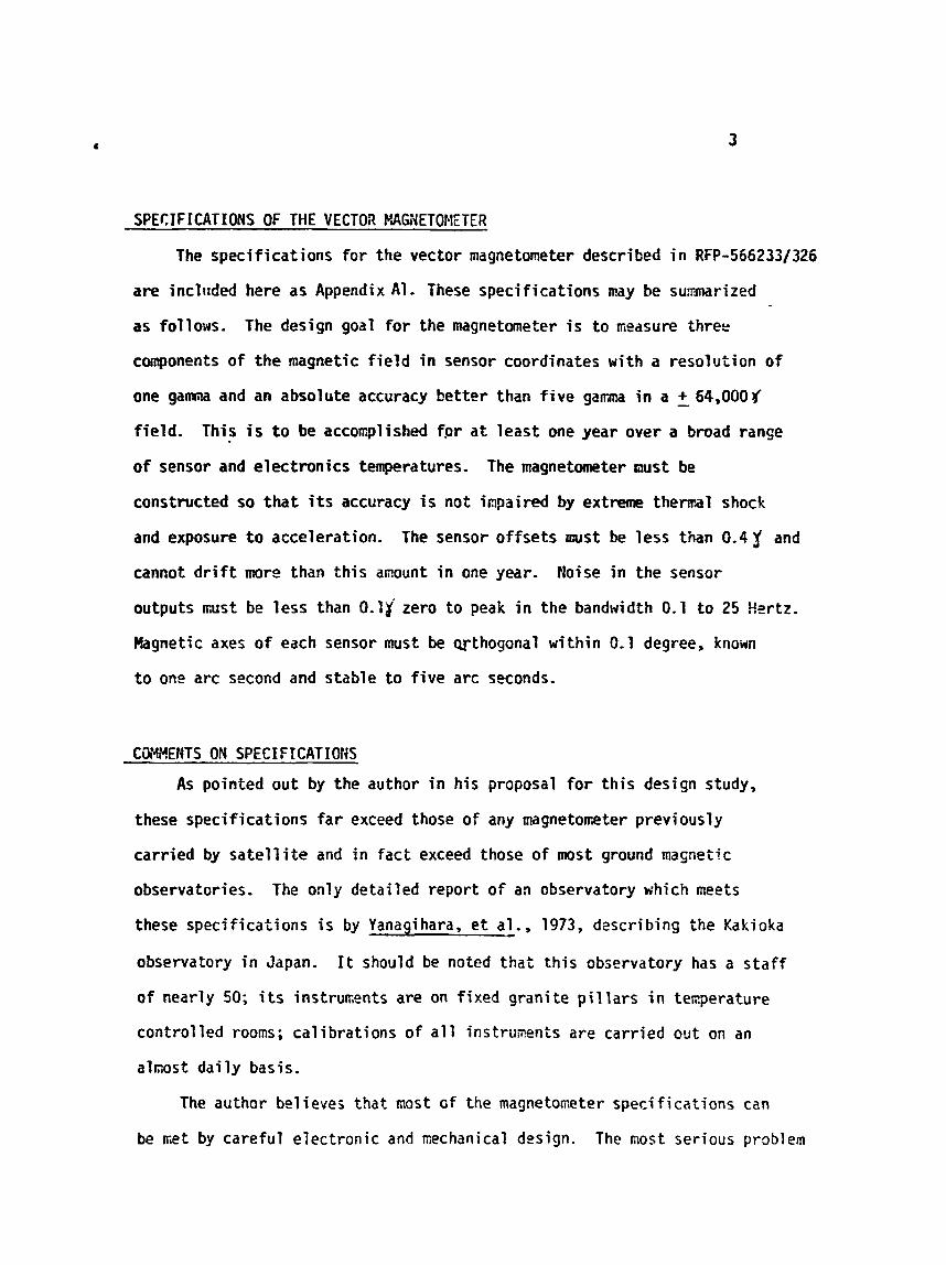
SPECIFICATIONS OF THE VECTOR PIGYETOMETER

The spec i f ica t ions f o r the vector magnetometer described i n RFP-5662331326

are included here as Appendix Al. These speci f icat ions nay be su ,wr ized

as follows. The design goal f o r the magnetometer i s t o measure three

components o f t he magnetic f i e l d i n sensor coordinates w i th a reso lu t ion o f

one gamma and an absolute accuracy be t te r than f i v e ganma i n a - + 64,000g

f i e l d . This i s t o be accomplished for a t l e a s t one year over a broad range

o f sensor and e lect ron ics temperatures- The magnetometer must be

constructed so t h a t i t s accuracy i s not impaired by extreme thernal shock

and exposure t o acceleration. The sensor o f f se t s must be less than 0.4 1 and

cannot d r i f t more than t h i s amount i n one year- tioise i n the sensor

outputs must be less than 0 -11 zero t o peak i n the bandwidth 0.1 t o 25 H l r t z .

Magnetic axes o f each sensor must be wthogonal w i t h i n 0.1 degree, known

t o one arc second and stable t o f i v e arc seconds.

CiXYHENTS OM SPEC1 FICATIONS

As pointed out by the author i n h is proposal f o r t h i s design study,

these specif icat ions far exceed those o f any magnetoireter previously

car r ied by s a t e l l i t e and i n f a c t exceed those o f most ground m a ~ n e i i c

observatories. The only detai led report o f an observatory which w e t s

these spec i f ica t ions i s by Yanagihara, e t al., 1973, describing the Kakioka

observatory i n Japan. I t should be noted t ha t t h i s observatory has a staf f

o f nearly 50; i t s i n s t r u ~ e n t s are on fixed gran i te p i 1 l a r s i n t e ~ p e r a t u r e

cont ro l led rooms; ca l ibra t ions of a l l instruments are car r ied out on an

almost d a i l y basis.

The author believes that most of the magnetometer spec i f ica t ions can

be ~ e t by carefu l e7ectronic and riiechanical design. The nost serious problem

however, is angt~lar calibration and s t ab i l i t y of the sensors. For example,

according to Yanagihara e t a1 . , 1973, ordinary magnetic theodol i tes can

determine the direction of an unknown f ie ld to no better than 6 arc seconds.

A specially bui 1 t theodolite i n use a t Kakioka (A-56, universal standard

magnetometer) could only obtain 3 arc seccnd accuracy. A more recent

version of t h i s instrument, the 01-72 has obtained an accuracy of one arc

second.

I t goes without saying that the accuracy of a calibration can be no

bet ter than that of the t e s t fac i l i ty . Thus, from the preceding discussions

i t would appear that the calibration of the orientation of the t e s t coi l

w i l l be limited t o about 6" unless special equipment i s available. T h i s

i n turn \~ould impose a similar e r ror on the magnetometer calibration,

In t h i s report we develop an a1 ternative procedure for a n g u l a ~ calibration

tha t does not require a magnetic theodol its. Instead, we use measurerrents

made by the sensor under calibration to sinultaneously detemine the

oriepc3tion of both the t e s t coil and sensor- As we will show, t h i s

procedure i s limited by the accuracy w i t h which the magnitude of the

calibration f ie ld can be wasured and by the accuracy of the sensor's

sensi t ivi ty and cf fse t .

DESCRIPTION OF TEST FAC I L 1 TY

To meet the specifications of Appendix A1 i t will be necessary t o

carry out the magnetometer c a l i b r a t i ~ n in a well calibrated rcagnetic

t e s t fac i l i ty . A t the present time there are only two such f a c i l i t i e s

i n the U.S., one a t Goddard Space Flight Center and one a t the h i e s

Research Laboratory. The Amps fac i l i t y has a rather small s e t of calibraticn

coils and no provisions for thermal -vacuum calibration, consequently,

we will assure that the test will be carried out at GSFC.

A brief s u m r y of some of the facilities available at GSFC for

magnetomter testing is given in a report by C.A. Harris, 1971. The

magnetic field component test facility consists of a 22 foot diameter

three component coi 1 system with remtely isolated magnetometer and

control instrunentation buildings. The orthogonal field cancelling coils

are sufficiently large that nearly any magnetic field may be produced in

a sphere of diameter 3 feet. The main winding of each roil is connected

to one axis of a 3 axis resonance magneto~eter which senses the variations

in the earth's field and feeds back a current which cancels this field.

The main winding is also co~nscted to a D.C. field generator which can - produce fields of up to 60,0003 in O.1$ steps. A sec~nd winding on each

coil is used to cancel the temperature depe~dence of the ~ a i n winding.

A third winding is used to mimimize field gradients over the test

vol urn.

The orthogonal coils are oriented with X horizontal towards ~agnetic

north, Y horizontal to the east, and Z vertically downward. The field

generators can produce 60,0001 i n 2 , 25,0003 in X and 6,000$ in the east-

west direction. Accuracy of field nu1 ling is of order 0.23. The gradients

across the 3 foot test volu32 are such that the field does not depart

from the center value by more than 0.65.

DESC!? IPTION QF TLST EOU I PMENT --

Several pieces of test equipment o f high precision and accuracy are

required to carry out the calibrations o f the test facility and magn~tonieter.

In th is report we asslane the following items are available.

1) 6 digi t - digital volfmeter

3 preci sion resi stors

Proton precession magnetometer

2- 3 component station magnetometers

2 - Optical theodol i t e s (autocoll imaters)

2 - Precision levels

Optical octagon

Brass fixture for rotating sensor assembly

Programnable digital data logging system w i t h analog and

digital inputs a s well as keyboard entry

Calibration of Test Facility

To accomplish the absolute accuracy required by the mission requirements

i t is necessary to calibrate the t e s t fac i l i ty f i r s t . Steps i n t h i s

procedure are described i n the fo1 lowing subsections.

Measure Cali bration Coil Constants

Place a precision resistor i n the current loop from the DC f ield

generator to the main winding of each coil. Pionitor the voltage drop

across the resistor with the digital vol tmter . F i x the proton precession

magnetometer a t the center of the t es t volum. Increment the f ield

generator in 5000 steps across the full range of the proton precessign

magnetometer ( Z 20,000-60,0003). For each step record the f ield measured

by the proton magnetometer 10 t i w s and average. Also record the reading

o f the digital voltmeter and convert to current using the known resistance.

Repeat for the sarre range of negative field values.

F i t ti st ra ight 1 ine t o the f i e l d versus current data determining

the c o i l constant (slope] and c o i l offset (intercept). B = k1 + Bo.

Also determine the probable errors i n these constants using the known

accuracy of the precision res is to r and d i g i t a l voltmeter as wel l as the

standard deviation o f the proton magnetometer measurements. Assign a

probable er ro r t o any t e s t f i e l d calculated on a basis o f t h i s formula.

I f the c o i l o f f se t i s not zero o r thore are systematic departures o f

the f i e l d from . - the . l i nea r . re lat ionship then a more elaborate ca l ibrat ion

w i l l be required. This p o s s i b i l i t y exists since the ca l ib ra t ion f i e l d

generator output i s mixed wi th the output of the resonance magnetometer

which nu l l s the earth's f ie ld .

Minimize Ca1ibration:Coi 1 ~ r a d i e n t s -.

Set the maximum possible f i e l d i n a c o i l - Use the proton precession

magnetometer t o measure the f i e l d along the c o i l axis a t 6 inch intervals.

F i x the magnetometer a t the point o f maximum deviation from the center

value. A1 t e r the current i n the gradient adjustment coi 1s t o reduce t h i s

deviation as much as possible. Repeat the survey along the c o i l axis.

Agafn, f i x the magnetometer a t point o f maximum deviation and again adjust.

I te ra te t h i s procedure u n t i l the f i e l d i s as unifontr as possible.

Test Earth F ie ld Nul l ing System

The earth's f i e l d nu l l i ng system i s a servo loop w i th the sensors

physical ly separated from the region i n which the f i e l d i s being nulled.

Inevitably there are small differences i n f i e l d between these two locations

whim the sensors cannot measure. Because o f t h i s there w i l l be a saall ,

resjdual f ield a t the center of the coil system. This f ield will have both

constant and time varying components. The magnitude of these components

limits <he accuracy of any magnetometer calibrations. The residua1 f ie ld

can be measured i n the following manner.

Place a calibrzted three component fluxgate magnetometer a t the center

of the coil system. Align the sensors roughly along the coil axis.

Record the output of t h i s magnetometer w i t h the digital data acquisition

system.

Perform three series of measurements. First, record about 1 minute

of data a t a sample rate exceedit~g 120 samples per second. Next record one

hour of data a t a sarilple rate o f 2 samples per second. Finally record 8

hours of data a t a sample rate of one sample per 5 seconds. Repeat th is

series of measurements for the fol 1 owing conditions : Midweek workday,

midweek n i g h t sh i f t , weekend midday, weekend night shift .

The data gathered i n the foregoing experiments should then be subjected

to power spectral analysis. For each se t of conditions separate auto

spectra are calculated for data a t each sample rate. These auto spectra

can then be plotted as log power versus log frequency on the sace

graph. The data define the magnetic noise i n the t e s t fac i l i ty from

about 0.3 millihertz to 100 Hertz. A separate graph for each se t of

conditions show how this noise i s a function of time during the work week.

To define the expected error i n any particular magnetic f ield m, ~asu re -

rent we integrate under the appropriate noise spectrum. For a lowr frequency

limit use the reciprocal of the duration of the measurement (the t i m ? during

which we must assume the field is constant). For an upper l imit use the

Nyquist frequency of the magnetometer making the f ie1 d measurement. The

rms field error i s the square root of the area under the noise power curve

between the specif ied l imi ts.

Oef ini tion of Geographic Coordinates

Test procedures described below require the definition of an accurate

geographjc coordinate system. T h i s can be done as described below.

A t e s t table is installed i n the center of the to i l system with i t s

surface about six inches below the center l ine of t h e horizontal coils.

The table should be made of either granite, marble or glass. I t must be

nonmagnetic and rigidly attached to pylons sunk to br-drock. I t should

have provision for adjusting the surface using precision levels t o be

exactly level. The table should also provide a means for rigidly

attaching a straight edge to the surface of the table. (This is used

where repetitive measurements with 180" rotation are required. )

Once the t es t table i s installed and leveled the geographic coordinate

system is established w i t h the use of two theodolites as-shown i n figure 1.

The f i r s t theodolite i s placed north of the t e s t table on a s t ru t or pylon

sunk to bedrock. T h i s should -- not be one o f the fixtures holding the

calibration coils. Later i t will be important to determine the orientation

of the coil axis in geographic coordinates. This can not be done i f the

theodolites are attached to the coil supports.

The theodolite i s leveled by placing a mirror on t h z test table a t

the exact center o f the tes t coils. The mirror i s gradually rotated (with

tangent screws) until the reflected beam i s observed in the theodolite.

The theodolite i s translated vertically and horizontally u n t i l i t i s

level with the telescope in the same plane as the mirror.

A second theodolite i s placed a t the same distance as the f i r s t b u t to

the east of the coil center. The mirror i s replaced by a right a n g l e

reflector. The second theodolite i s translated until a beam from the f i r s t

enters the second theodolite when i t i s exactly level.

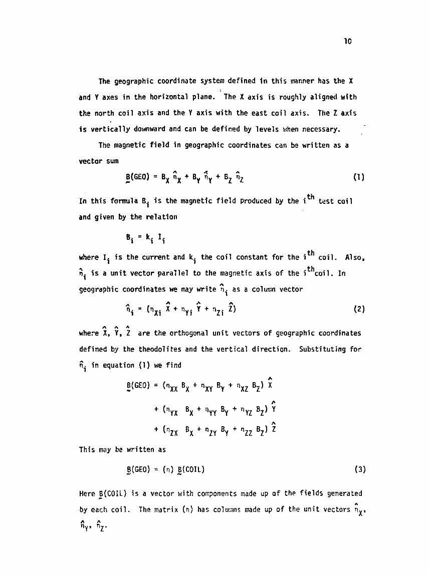
The geographic coordinate system defined i n t h i s manner has the X

and Y axes i n the horizontal plane. The X axis i s roughly aligned w i th

the north c o i l ax is and the Y axis w i th the east c o i l axis. The Z axis

i s ve r t i ca l l y downward and can be defined by levels when necessary.

The magnetic f i e l d i n geographic coordinates can be wri t ten as a

vector sum

I n t h i s f o m l a Bi i s the magnetic f i e l d produced by the ith tsst c o i l

and given by the re la t ion

where Ii is the current and ki the c o i l constant f o r the ith coi l . Also,

Gi i s a u n i t vector para l le l t o the magnetic axis o f the i thcoi l . I n

yographic coordinates we my wr i te Gi as a column vector

A A A

where X, Y, 2 are the orthogonal u n i t vectors o f geographic coordinates

defined by the theodolites and the ver t i ca l direction. Substituting f o r

ti i n equation (1) we f i nd

This may be wr i t ten as

Here 6(COIL) is a vector with components made up of the f ie lds generated C

A

by each c o i l . The m a t r i x (n) has co1u:nns made up o f the u n i t vectors ox,

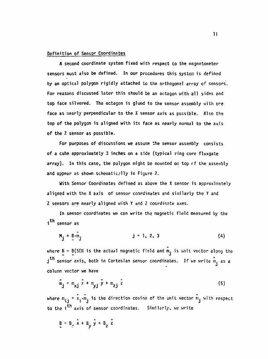
Definition of Sensor Coordinz tes

A second coordinate system fixed w i t h respect to the magneton:eter

sensors must also be defined. In our procedures this system is defined

by an optical polygon rigidly attached to the orthogonal array o f sensors.

For reasons discussed l a t e r t h i s should be an octagon w i t h a l l sides and

top face silvered. The octagon is glued to the sensor assembly with ore

face as nearly perpendicular t o the X sensor zxis as possible. Also the

top of the polygon is aligned w i t h i t s face as nearly normal t o the axis

of the Z sensor as possible.

For purposes of discussions we assume the sensor assembly consists

of a cube approximately 3 inches on a side (typical r i n g core fluxgaie

array). In t h i s case, the polygon might be mounted on top r f the assenbly

and appear as shown schematic~lly i n Figure 2.

With Sensor Coordinates defined as above the X sensor i s approximately

aligned w i t h the X axis of sensor coordinates and similarly the Y and

Z sensors are nearly aligned w i t h Y and Z coordinzte axes.

In sensor coordinates we can write the magnetic f ie ld measured by the

ith sensor as

A

where 8 = B(SEN is the actual magnetic f ie ld and m. i s unit vector along the - " J jth sensor axis, both i n Cartesian sensor coordinates. I f we write n. as a

3 column vector we have

-- - where mi - - Xi*mj

is the direction cosine of the unit vector m . w i th respect J

t o the i th axis of sensor coordinates. Similarly, we write

Substituting i n equations (4) we obtain

This my be writ ten i n matrix form as

The matrix (p) i s a matric whose colunars are t5e u n i t vectors ~ long the

magnetic axes of the three sensors. The vector # i s a vector w i t n cmpcments - ~ i v e n by the act-: m e a s u m t s aade by the three sens~&s. The inverse of

eq. (6) allows one to obtain a Cartesian vector f r ~ m the actu i l masurments, i ,e,

I t should b2 noted that the vector # i s not the representation o f - the actual aragnetic f i e l d i n a non-Cartesian coordinate system aligned w i t h

the sensor axes. I f we want t h i s representation we m s t m i t e

Rearrmging terns t h i s becorns

here B(IIEA) = (BXa, , B ) i s the representation o f 6 i n the nm- - - Cartesian coordinate system aligned uith the magnetic axes o f the sensors,

Using the result, eq. (6) we f i nd

o r f i n a l l y

Prepar3tion of bgnetometer Test Fixture

The test procedures discussed below require that the sensor asreably

be oriented i n a variety, o f precisely known orientations re lat ive t o

geographic coordinates. This i s accorspl i s M by r i g i d l y attaching an

optical polygon to the sensor assembly, Reflections from the faces o f

these polygons are m i t o r e d by the two theodolites and used t o calculate

the precise orientation of the polygon. The d i f f i c u l t y w i t b t h i s procedure

r S the l imi ted f i e l d o f view o f the t9eodolites. It i s not possible t o

perfom arbi t rary reorientations o f the sensor asseabiy and have a face

o f ehe polygon nearly n o w 1 (within about a ha1 f degree) o f the t k o d o l i t e

optical axis.

To solve the foregoing problem we u t i l i z e a magnetmeter tes t f i x t u re

which makes possible reaso~ably accurate rotations about two orthogonal

axes. An example of such a f ix ture i s show i n Ffgure 3. The device

shorn i s an earth inductor or magnetic theodolite. I t s purpose i s the

accurate determination o f the direction o f an unknown magnetic f ie ld .

It u t i l i zes a spinning search co i l t o indicate when the search c o i l

rotat ion axis i s a l i p e d with the aarbient f ield. The azimuth and elevation

of the rotation axis are *ad from horizontal and vert ical circles.

~e propose t o tnodify such a device as s b schematically i n f igure 4

The search coi 1 dr ive asse=bly i s replaced fy hollow tubes concentric

w i t h the elevation axel (horizontal axis). This allows unobstructed

observation of me face of the opt ical octagon when mitnted with in the

f ixture. The search c o i l i s replaced by a mounting plate with attachjlent

claapr. The platform and c l a p s are provided w i t h adjusts#nts which enable

the experinentor to a l ign the optical axes o f the polygon w i t h the rotat ion

axes o f the fixture.

The procedure f o r sett ing up such a f ix ture warid be as described

below. Place the magnetmeter sensor as red ly on the m n t i n g plate o f

the f ixture. The plate should be designed such that the center o f the

optical polygon i s close to the intersection o f the vert ical and horizontal

axes o f the fixture. Place the f ix ture on the test table wi th the

norizontal axis pointing north and the center o f one face o f the octagm

i n l i n e with t!~e north theodolite. Hove the f i x tu re along the north-

south 1 ine u n t i l the center o f an orthogonal face i s roughly a1 igned w i t h

the east theodolite. Level the f i x tu re using the three level ing screws

and levels a t t a c W t o the base o f the f ix ture- Rotate the f i x tu re i n

az imth w i t h a tangent screw u n t i l the nonnal to the northward face l i e s

i n a vert ical plane passing through the north theodolite. Next, use the

adjustment screws on the mounting plate to bring the n o w 1 to the east

face in to a vert ical plane passing through the east theodolite. Repeat

these steps u n t i l both fazes o f the polygon are nearly orthogonal to the

two t!teodolites. Hhen thi: i s achieved the top surface of the polygon shoo7ci

be almost level.

Wc#r continue with fine adjus-nt of f ix ture level t o bring the

azimuth axel (wertjcal axis) vertical. Do th is by rotating i n azirnrth

by 45" incresents. If the successive faces do not produce centered images

i n the theodolites the azimth rotation axis i s not truly vertical. Rake

i t so by f ine adjustments o f fir'ure level,

Wen the foregoing procedure i s coapleted i t should be possible to

perform rotations through angles of integral multiples o f 4S0 and maintain

reflected issages o f crosshairs within the f ie ld o f view o f the t h e 1 i tes-

Because of the inaccuracies associated with the bearings o f the test

f ixture it i s not expected that the rotation axis w i l l be stable to mch

better than stme fraction of a minute of arc- Also errors associated w i t h

the verniers on the azimuth and elevation circles w i l l l i m i t the accuracy

o f rotation angles t o same fraction o f a minute.

This problem i s not iaqrortant. Actual aligment of the sensor coordi-

nates i n geographic coordinates i s detelPnined by the theodolite reflections

frun the precisely constructed faces o f the optical octagon. The prisary

purpose o f the f ix ture i s t o provide suff iciently accurate rotations that

the reflected imgss m a i n within the f i e l d of view o f the tkeodolites.

Relation between Sensor and Geographic Coordinates

I n the previous section we described a procedure for setting up a

test f ixture which holds the array of sensors to be calibrated. The

sensor assembly has attached to it an optical octagon with i t s top and

side faces silvered. The faces o f th is octagon must be constructed so

that they meet a t 45" angle and are f l a t to better than one arc second.

The top must be a t 90' to a l l faces w i th in the same accuracy. The f ixture

i s su f f i c i en t l y precise tha t i t can rotate the sensor assembly through

angles i n incremnts of 45" so tha t irages ref lected t o the theodolites

viewing t h e orthogonal faces of the octagon t-emain i n the f i e l d o f view.

I t i s not expected that these images w i l l be exactly centered. The exact

or ientat ion i s thus determined by using the theodolites as eutocol l inators

readiag the precise or ientat ion t o a f ract ion o f an arc second.

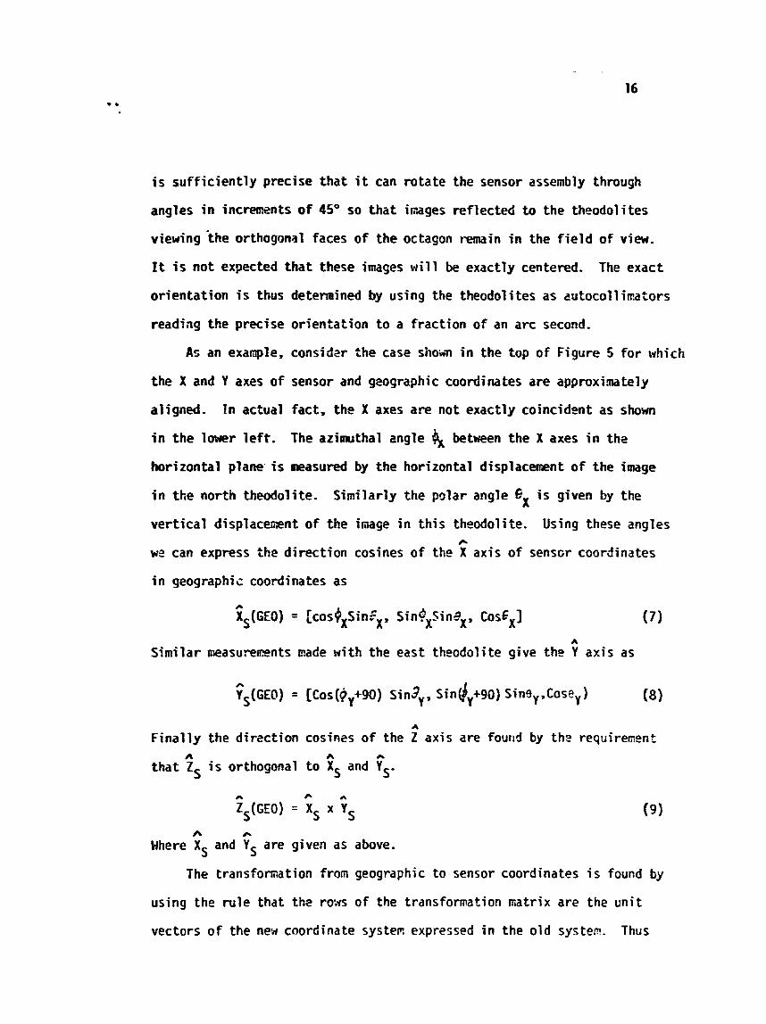
As an example, considzr the case shoii i n the top o f Figure 5 f o r which

the X and Y axes o f sensor and geographic coordinates are approximtely

aligned. I n actual fact, the X axes are not exactly coincident as shown

i n the lower l e f t . The azimuthal angle 4 between the X axes i n th.

horizontal plane- i s u i e a s u ~ by the horizontal displacemnt of the image

i n the nortb theodolite. S imi lar ly the p ~ l a r angle GX i s given by the

ve r t i ca l displacewnt of the imp i n t h i s theodolite. Using these angles f i

w? can express the d i rect ion cosines o f the X axis o f sensGr coordinates

i n geographic coordinates as

A

Similar ineasureents mde wi th the east theodolite give the Y axis as

A

F ina l l y the d i rect ion cosines o f the Z axis are found by th: requirment n A A

tha t Z S i s orthogonal t o XS and YS.

h 6

Where XS and YS are given as above.

The transfornation from geographic t o sensor coordinates i s found by

using the ru le that the ro-.qs o f the transformation matrix are the u n i t

vectors o f the new coordinate systen expressed i n the o ld systen. Thus

E(SEN) = (R) !(CEO)

where -

Successive rows of (R) are given by the elements of t h s vectors appearing

i n equations 7, 8, and 9 respectively.

W i t h the results presented above and i n previous sections w? czn

easily relate the niasured magnetic field to the field produced by the t e s t

substituting equation (3) into (10) we hzve

then, substituting t h i s result i n eqoation (6) we find

Equation (12) graphically i 1 lusiratss the fact t h i t any measurecnt

made i n the calibration facility couples the u~known direction ccsines

of both the coil and the nqnetometer axes. Also i t i s apparent t h a t t h i s

equation is nonlinear i n the unknoms. I f we perfom a nunb2r of experircents

creating a s e t o f such equations xe m s t solve a s e t of simltzneous, non-

linear equations. This problem is further coxplicated by the fact t h a t

each column of ( v ) and (r,) i s a unit vector, i.e. there are only 2 unknw.ms

rather than three per column. Thus, altogether there are 12 unknobins to

be determined experimn tal ly. A procedure for acco~pl i shing tfiis i s

described i n a subsequ~nt section.

CALIBRATION OF IMDIVIDUAL SENSORS

The second major step of the vector magnetmter calibration procedure

i s ttie calibration of individual sensors. This calibration includzs the

determination of sensor sensitivity offset, noise and dr i f t . In add4 tion,

i t involves the measurecent of the effects of temperature and magnetic

fields orthogonal to the sensor. In following subsections we discuss each

of these procedures i n detai 1.

Htasurmen t of Sensor Sensitivity and Monl i neari ty

The coinponent of magnetic field parallel t o the axis of a linear

fluxgate sensor may be written

In th is equation Yi i s the sensor sensitivity in gama/volt, and Oi

i s the sensor offset i n g a m . To determine thsse constants we nust

apply known magnetic fields B and measure the sensor output voltage, Yi (By).

Plotting the applied f ield as a function of output voltage, the slope o f

a best f i t straight l ine determines the sensitivity 2nd the intercept

determines the offset, Oi. Systematic deviations of the measurements from

the best f i t line indicate t h a t the sensor i s not truly linear.

Momlly, the sensitivity of a magnetomter is deteminsd from

only two sets of ~easurewnts , one a t zero field and one near ful l range.

I n the following paragraphs we show this procedure is not sufficiently

accurate to met t h 2 requirement of 1 gama absolute accuracy over the

full dynzmic range of the sensor. Consequently, i t is necessary to mke

a large nuzber of measurements across the full dynamic range of the sensor.

These ~ e a s u r e ~ e n t s are then f i t by a least square straight line. This

procedure inproves the accuracy of the sens i t i v i t y determination and has

the addit ional advantage that a p l o t may be made o f the deviation o f the

observations from the best fit.

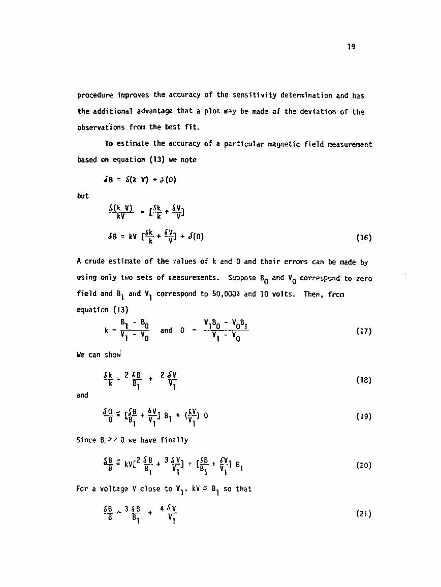
To estimate the accuracy of a par t i cu la r magn2tic f i e l d ~easurenent

based on equation (13) we note

but

A crude estimate of the values of k and 0 and t h e i r errors can be made by

using oniy two sets o f s~easurenents. Suppose BO and Vo correspond t o zero

f i e l d and B1 artd V1 correspond t o 50,0003 and 10 vol ts. Then, fmm

k = Bl - and 0 = v lBO - Y ~ B 1 - vo v~ - We can show'

and

Since B, > 7 0 we have f i n a l l y

For a voltag? V c lose t o V,, kV = B1 so tha t

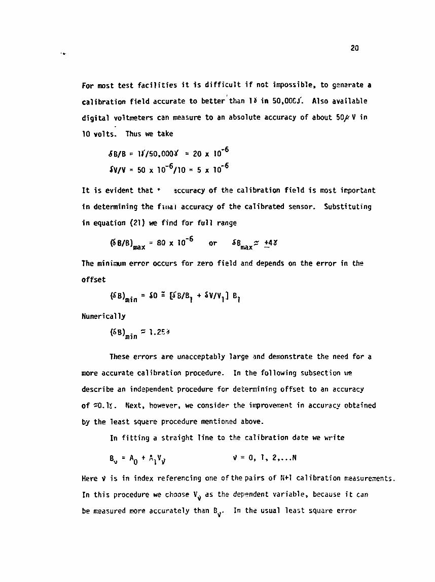
For most tes t fac i l i t ies i t is diff icult i f not impossible, to gentrate a

calibration f ield accurate to better than 1 8 in 50,00G~'. Also available

digital voltmeters can measure to an absolute accuracy of about 5 0 1 V i n

10 volts. Thus we take

I t is evident that + sccuracy of the calibration f ield is rrast icqortant

i n determining t h e f itla i accuracy of the calibrated sensor, Substituting

i n quation (21) we find for full range

The miniam error occurs for zero field and depends on the error i n the

offset

Numerical ly

These errors are unacceptably large and demnstrate the need for a

more accurate calibration procedure. In the following subsection

describe an independent procedure for determining offset to an accuracy

o f s O . l S . Next, however, we consider the intproveirent i n accuracy obtained

by the least squere procedure mentioned above.

In f i t t ing a straight line t o the calibration date we rite

8, = AD + AIVJ J = 0, 1, 2, ... N

Here ? i s i n index referencing one of the pairs of N+1 cal i bration rrteasurenents.

In th is procedure we choose Y* as the dependent variable, because i t can

be measured more accurately t h a n Bv. In the usual least square error

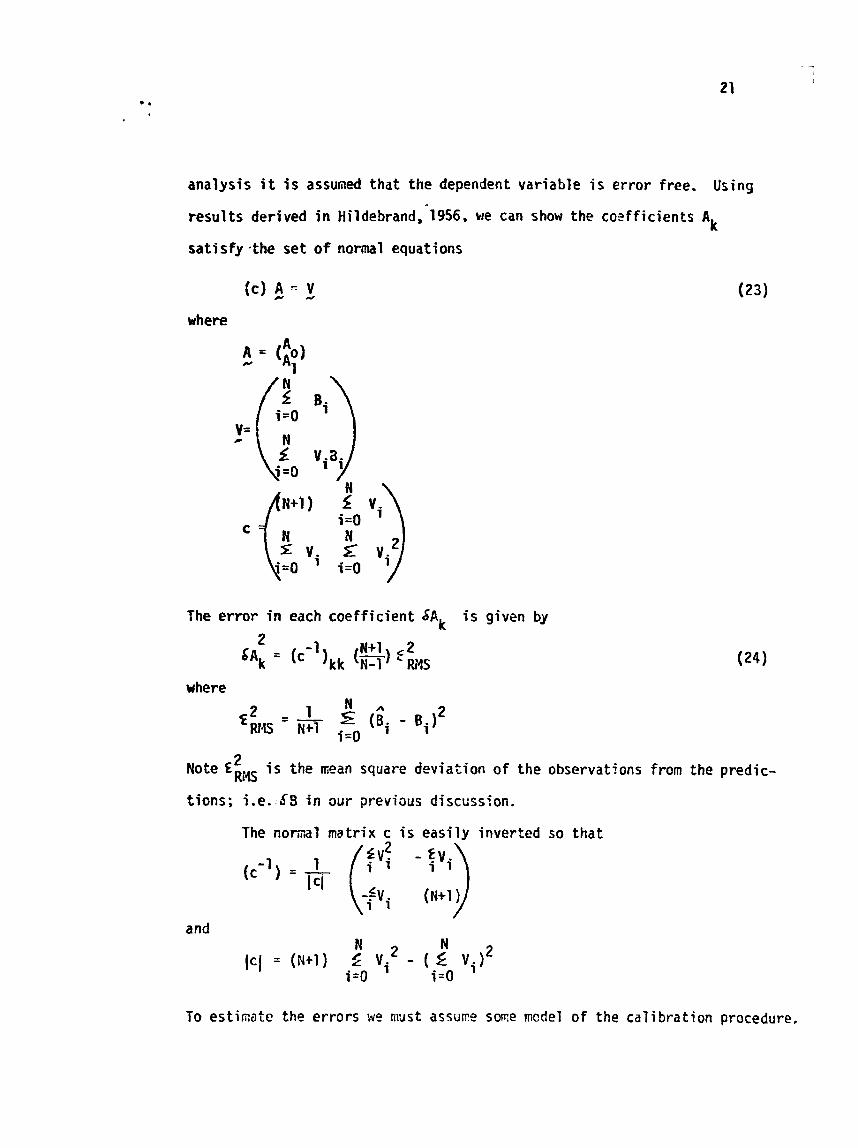
analysis i t i s assumed tha t the dependent variable i s error free. Using

results derived i n ~ildebrand~"l956, we can show the coefficients Ak

sat is fy -the set of normal equations

Ic) 4 = y where

The error i n each coefficient &Ak i s given by

where

2 Rote EILyS i s the mean square deviation of the observations from the predic-

tions; i . e . -63 i n our previous discl;ssion.

The nomil matrix c i s easily inverted so tha t

1 (C-') = - I =I

and

To estimate the errors we must assure sme mcdel of the calibration procedure,

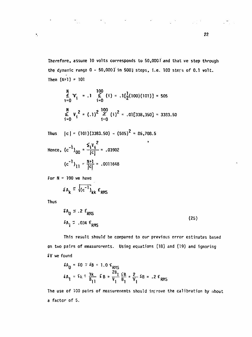
Therefore, assume 10 volts corresponds to 50,000~~ and that we step through

the dynamic range 0 - 50,000$ i n 5003 steps, i.e. 100 s t e r s of 0.1 volt.

Then (N+l ) = 101

N 100 5 V- = 1 b ( i ) = .1[~(100)(101)] = 505

i =O 1 i =O

Thus l c 1 = (101)(3383.50) - ( 5 0 5 ) ~ = 85,708.5

4vi 2 -i - Icl

- ,03902 Hence, (c )00 - - -

For N = 100 vie have

Thus

T h i s result should be conpared to our previous error estimates based

on two pairs of neasure~enis. Using equations (18) and (19) and ignoring

SV we found

gAo = SO ~ I B = l.OERMS

The use of 100 pairs of measurements shou ld irnjrove the calibration by ;,bout

a factor of 5.

The er ror i n a f ie ld measurement was according t o equation (16),

= kV [a+ q] + S O k

since SAo = 50 and Sk = $A, we have

4 $8 = 5 x 10 16.8 x ~ o - ~ E ~ ~ + 5 x + .2 EwlS max

If ENS = 1x.

a h a x - .6 + .2 = .8Y

While the foregoing error is quite acceptable i t depends on the

l ineari ty of the magneto~ter . If the observations systematically depart

from a s t raight l i ne gRhlRMS will be larger than 13, and SB will be max

proportionally larger. In this car0, it might be necessary to use higher

order functions t o f i t the cbservations.

On a basis o f the preceding analysis kie recornend the procedure

shoVm schematically i n figure 6, t o determine sens i t iv i ty and offset of

each sensor. Attach the sensor to a t e s t f ixture which has provisions fo r

s l ight rotations of the sensor about two axes. Place the fixture on the

t e s t table with one edge against a north-south s t ra ight edg? attached to

the table. Apply maximum f ie ld (250,000~) i n the north direction.

Rotate the sensor around a vertical axis t o obtain maximcm output voltage.

Next, rotate the sensor about a horizontal axis again maximizing the

output voltage. Repeat these steps several times until the best possible

alignnent of sensor magnetic axis and calibration f i e ld i s obtained.

Once a l i y w n t i s achieved perform a sequence of measurements

deiemining sensor output voltage as a function o f cal i bration magnetic

f ie ld. To deternine the precise input f ie ld use a digi ta l voltmeter t o

monitor the voltage d r o p across a precision res i s tor placed in the f ie ld

generation drive c i rcu i t . Using the c a l i b r ~ t i o n coil constant determined

by t h e ~ e t h o d described above and the ~easured coil current

(ICOIL = V/R) calculate the applied field. Also use the digi ta l voitmeter

to measure the sensor output voltage corresponding to the i n p u t f ield.

To obtain sufficient accuracy perform 101 pairs o f measurecents w i t h

the i n p u t f i e ld increnented i n 1000 steps over the range -50,000 t o

+50,00Of. Enter ihr table o f neasure~snts, Bi versus Vi in to a computer

program which f i t s a least square l ine to the data determining k , 0 and

t h e i r associated errors. The p r ~ q r z n she, d also calculate and plot the

deviation of the predicted f ie ld from the observed field. I f the resulting

time series is Gaussian w i t h zero mean the sensor i s linear.

T h i s procedure i s repeated twice more for the reixaining two sensors.

Together these three exper i~ents define the sensi t ivi t ies and offsets

required to measure the three components of the magnetic f i e ld provided

the orientation of each sensor i s known i n iner t ia l space.

Measurernent o f Sensor Offset i n Low Flela

An ind\!pendent, and more s e r , ~ i t i ve determination df sensor o f f se t

can bc made by tes ts performed i n a lo\* f i e l d environment. This procedure

i s somewhat easier than the one described i n the preceding sbbsection

and because i t does not require a large t e s t f a c i l i t y , we reconlrnend

t ha t i t be used f o r long term moni tor i rg o f temporal d r i f t s i n offset.

The sensor o f f s e t i s defined by e q ~ ~ a i i o n (13)

B = k V + O

Solving for the magnetometer output voltage we f i n d

Suppose vie piace the sensor i n a1 ignnent w i t h a weak f i e l d B the sensor 0 ' output w i l l be

Now reverse the d i r ec t i on o f the f i e l d e i t h ~ r by a 180 ro ta t ion o f the

sensor o r by changing thz sense o f the c u r r ~ n t producing th2 f i e l d . The

output voltage i s

Adding the two measurements and solving f o r 0 we have

Note tbe s e n s i t i v i t y must b2 independently determined t o calculate o f f se t .

The e r ro r i n 0 i s roughly

6 from equation (25) Sk/k 2 7 x 10- . Hov~zver SV/V i s o f order 1. The

di f ference i s t ha t d~ should not be t h e precis io i l o f the neasurenent dwice,

but the f l uc tua t ion induced by var iat ions i n the anbient field and by

i n s t m n t noise. I n an unshielded. industr ia l envirozzent f luctuat ions i n

wol tage SV correspond t o f i e l d f luctuat ing o f order 15- Since r i n g core

of fsets are o f the sarse magnitude ~l;e expect dY - V- Clearly accuracy can

be obtained only by repeated measuremts i n a shielded environent.

To carry out a detemination o f o f f se t we r e c m n d t!x following,

Place the sensor on a f i x tu re which allows an approximate 180° rotation,

(An accuracy o f a few degrees i n t h i s rotat ion i s suff icient,) Place the

sensor and f i x t u r e inside a set of concentric nu metal cans- Cpver

each can w i th i t s eu e t a 1 cap :xsluding the earth's f i e l d from the

i n t e r i o r o f the innernost can. A remanmt magnetic f i e l d o f a few g x m a

magnitude and unknm direct ion w i l l re ra in i n the can. Since the d i rec t ion

o f t h i s f i e l d cannot be chcnged the orientations o f the sensor m s t be

reversed- Per fom a series o f w-suremnts o f tk asgn&amter out?ut

vol tag?, ro ta t ing the sensor 180° before each seasurenl2nt. Procegaini,

through ttr? table o f e z s u m n t s , average pai rs o f readings and calculate

offset. Average the offsets so de te rn i~ed t o obtain a f inal, %ore accurate

value.

Yleasure=nt o f Sensor Hoise i n Law Fie ld - In preceding sections we have discussed offset as if i t were a constant

property o f the sensor. I n fact, of fset usually changes wi th time i n a

random mnner. For fluxgate sensors, a frequency spectrum of these chacges

i s t yp i ca l l y inversely proportional t o frequency. Thus, on a short t i ne

scale, variat ions i n of fset are qui te s m l l . I n general, these var iat icns

are divided into t r ~ catagories depznding on t h e i r tie scale, Variations

which take longer than s0iT:e reference ti= are ca l led offset while thosz

that take less tim are called noise. A typical rc. 7ce time i s

betwen a day and a week.

Senscr noise i s best charactzrized by a power spectrum o f the sensor

output when located i n a zero f i e ld environment. In such a s i tuat ion i t can

be asstiiaed that a l l variations i n output are a resul t o f the i n s t n m n t

rather than the mbient f ie ld.

Ye suppose t h a t the sensor has k e n placed inside a set o f concentric

IBU metal cans as described i n the previous subsection- The sensor

output i s recorded by a d i g i t a l data acquisition system. Usually, i t i s

necessary to amp1 i f y the m a g m t e t e r output voltage p r i o r t o d ig i t i za t ion

or quantization noise created by Gigi i izzt ion w i l l dominate the speciru;s

a t h i g k r frequencies- Also i t i s i q o r t a n t t o low pass f i l t e r t h e sensor

output volZage wi th a time conshnt twice the sampling interval. This

eliminates the problem o f al iasing noise power from high t o low frequencies

i n the d ig i t i za t ion procedure.

Bemen 1000 and 5fX.J samples o f the sensor output s h n ~ l d be taken

2nd then read i n to a coqwter prograa f o r spectral analysis- This program

estimates the noise power i n a frequency band correspontiing to a h u t \O/T

t o 1/2ht where T i s the durat im o f the series o f measuremnts and tt the

sampling interval. For 5000 samples we have a r a t i o of upper t o lwr

frequency limits o f 250 or 2.4 decades o f frequency.

To cover a wider band o f frequencies i n an e f f i c i en t manner, be n i s t

repeat the above experiuent w i t h progressively higher saw? ing rates. A

convenient se t c?f experi1i:ents i s s m r i i e d schematically i n Figure 7.

The frequency band f rom Hertz (1 day) t o 50 Hertz (1M saq lcs per

second) can be covered i n three experiments. These are one dzy of recording

with one minute samples, one hour o f recording with one second sawles and

one minute o f recording with 100 sawles per second.

In order to consider the effects o f quantization noise i n th i s

mcasuremnt we m s t assuze SO^ typical noise spectruzi. for rcferecce i n

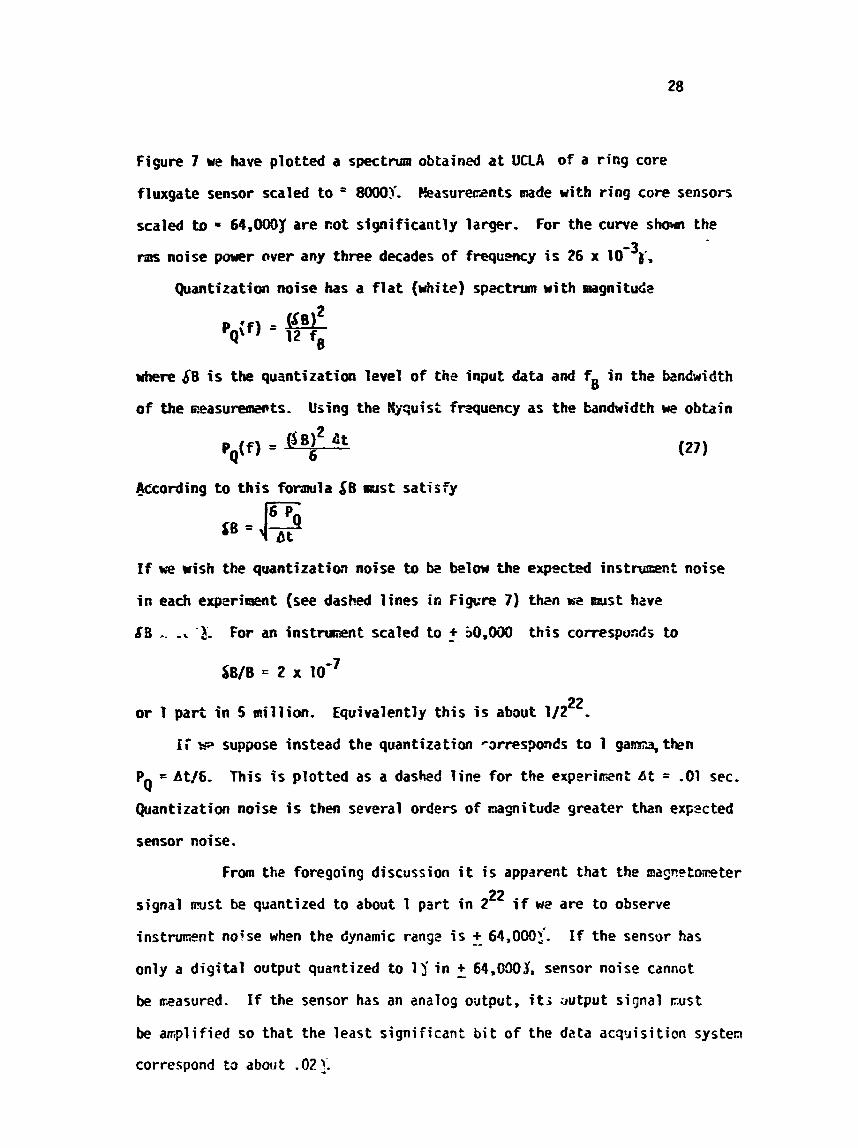
Ficpre 7 ue have p lo t t ed a spectrua obtained a t UCLA of a ring core

f luxgate sensor scaled to ' 80005. K e a s u r e r ~ n t s mde with r ing core sensors

scaled U - 64,0003 are cot s ign i f i can t ly larger . For t h e curve s h the

rsa noise power over any three decades of f ~ q u s l ~ y is 26 x 16~)~.

Quantization no i se has a f l a t (white) spmtrun with magnitudz

&re 6B is the qua t t i za t ion level of t h e input da ta and fg i n t h e bandwidth

of the mzasummmts. Using t h e Ayquist frequency as t h e bandwidth we obta in

&-cording to t h i s f o m l a $6 mast s a t i s f y

If we wish the quant iza t ion noise to k belaw expected instrunsent noise

i n each experiment (see d a s W 1 ines in Figcre 7) thzn e mst hzve

8% , . . For an i n s t m n t sca led t o - + 30,W t h i s c o r r e s p ~ n d s to

22 or 1 p a r t i n 5 a i l l i o n . Equivalently t h i s i s abaut 1/2 . i i w s u p p s e ins tead t h e q u a n t i z a t i m -wresponds t o 1 gam* then

p~ = At./6, This is p lo t t ed a s a dashed line for t h e experineni A t = -01 sec.

Quantization no i se i s then several orders of magnitude g r e a t e r than expected

sensor noise.

From the foregoing discussion i t is apparent t h a t t h e a a ~ o o t m t e r

s ignal mst be quantized t o about 1 p a r t i n 2** i f a2 a r e to observe

instrument noise when t h e dynamic ran52 is - + 64,000i. If t h e sensor has

only a d i g i t a l output quantized to 1 1 i n - + 64,090$, sensor noise cannot

be wasured. If t h e sensor has an analog oirtput, it; autput s ignal r ~ u s t

be amplified so t h a t the l e a s t s ign i f i can t b i t o f the da ta acquis i t ion system

correspond to about .02 5

For exmple, suppose, 50,0005 correspnnds t o 10 vo l ts - Then

-02 j = 4,4 volts. I f the data acquisi t ion system provi.?es a 16 b i t converter

over a ranse 0-10 volts, the least s ign i f i can t b i t i s 5 150p vcilts. An

amp1 i f ica t ion o f about 40 i s required t o tzeasure the sensor noise.

Our recotmended procedure for easur ing the noise o f th, sensors

i s srmtr;larized as follows, Place the sensor i n a shielded container. Low

pass f i l t e r and s-le the output s ignal- Record the smples on d ig i t 21

tape and subject the data t o spectral analysis- P lo t the resul ts as l o g

power versus l o g frequsncy, Three separate exper ien ts should be perfomed.

These correspond t o one day o f 60 second samples, one hour of one second

s ~ v l e s and 1 minute of -01 soizples- To be meaningful the effective

quantization o f the data should be abmt -02Y in 50,M)O? o r 1 p a r t i n 2".

I c l o a s u m t o f T m o r z l D r i f t i n Sensor Offset

In the preceding section rz pointed out tha t sensor o f f s e t i s tiire

varying. By def in i t ion, changes i n offset on a time scale l o n ~ e r than a

day are ca l led t q o r a l d r i f t - The d r i f t can only be masure0 by repeated

m e a s u ~ n t s a t widely separated times- Since i t would be d i f f i c u l t t o

rout ine ly carry out such masurernents i n a large tes t f i c i l i t y we retomend

use o f the l w f i e l d of fset determination procedure.

To determine the nature and magnitude o f t q o r a l d r i f t procezd 6s

follows. Cnce a week place a continuously operating three conionen: napeto-

w t e r i n the tes t f i x t u r e inside a shielded can. Carry out a series o f 180°

rotat ions and calculate offset. Repeat for the remining two axes. Retur:,

the magnetometer t o an isolated locat ion where i t continues t o monitor the

earth's f i e ld . P lot the three secsor offsets as a function of t i c ? f o r about

one year- A t the end of the year determine the wan offset and m s deviation

about the nean.

k a s u m t of Temp?rature Dtpendence of Sensi t iv i ty and Offset

I t is well established tha t the sensitivity as well as offset of flux-

gate magnetometers i s a function of temperature- Since the sensor electronics

i s separated frotlr the sensor assembly, both t h e electronics temperature

(TE) and t h e sensor t-rature (TS) are significant variables. Taking

t h i s dependence into account we rewrite equation (13) as

Considering t h e hro pararzters k and 0 as functions o f TE and TS we

wake the crude assumption

T ) + aJTE + b a s P(TE,Ts) = P(TEo, 50 e 9 )

In t h i s expression P i s either of the two paros~ters k or 0- The subscript

"0" designates t h e narninal operating tazperature (ass- moa temper2ture)

of the sensor and electronics. AT is then thi, deviation of e i t i e r W t r a -

ture from the nominal value. Finally, a and b are teqterature coefficients

OF the parmeter.

I t should not be expected that eqdation (29) appl ies over the full

range of operating temperatures for the ~ a g n e t m t e r . Experience a t UCIA

has shown thzt sensitivity is often a quadratic function o f both terrgeratures.

However, because of the rather 1 arge temerature dependaxe of typical

fluxgate sensors the N4r7SAT nagnetmter wi 11 certainly have t h e m 1

enclosures about both the sensor 3;seiribly and s e n s ~ r electronics. Uithin

t h i s enclosure teinperature variations should be so spa11 t h a t equation (29)

will be an adequate approxi~ation.

To determine the terperature dependence of k and 0 we proceed

a s follo\~s. Place the sensor assembly a t the center of a three axis

cat ibration coil faci l i ty. Align the three axes of t h e sensors as closely

as possihle with t h 2 three coil axes. Place thermal enctosores a b u t both

t h e electronics and the sensor assembly. Using hot and cold gases bring

both enclosures to nominal operating tecperatures. A1 low sufficient

t ime for both u n i t s to come to t h e temperature of their respective enclo-

sures (approximately one half hwr), Determine the sensor offsets and

sensi t ivi t ies for each axis by applying a sequence of co1 ibration f ields in

the appropriate calibration coil. Use least square procedures to calculate

ki and Oi. Keeping electronics buyeratwe constant increase sensor

temperature by 5O. A l l o ~ t h e sensor t o CORE to t h e m 1 equil ibrim, Again

carry out a series of ~easurentents deiemining k. and 0.. Rext, increment 1 1

sensor temperature by lo0, establish t h e m 1 equilibrium, and determine k i

and Oi. Finally, increment another and deternine ki and Oi. (Note

this sequence defines the paraneters for 8TS = 0°, 5 O . IS0 30°. ) Now

r e t u r n to nominal sensor teicperature decre-enting terperature by the saw

amsnts as it was previcusly incremnted- Continue t o negative

tezperature deviations usins the s 2 ~ 0 scheze C4T = -So. -lo0, -IS3).

Finally, return to nominal sensor teqerzture.

Plot the p a r a ~ t e r s ki and Oi as functions of T F i t straight S'

l ines to the three points a t ATS = -5O, O1. +So. The slope of these 1 ines

are the co2fficients b i n equation (29). The zero intercepts a r e the values

The for2going procedure i s no:* repeated holding sensar tespcrature

constant and varying electronics temperature. Again a plot is used to

determine the coefficient a in equation (29).

There i s a reizote possibility t h a t a l l three sensors might have

extrema for k i and Oi a t nearly the saze targerature. If th is were the

case i t k~ould be desirable to choose these c o m n teqera tures a s the nominal

operating teqcratures and repeat the seasurecent of a and b about th2se

new trt~peratures. I t shovld be sufficient to use only three te~peratures,

i - e . , bT = -So, O0 and +5". For these points t h e coefficients a and b wi l l

be smaller and the magnetomter s e n s i t i v i t y t o tanpera ture w i l l be

reduced:

Bkasummnt of Orthogonal Field Effec ts on S e n s i t i v i t y and Offse t

In t h e idea l i zed theory of t h e f luxgate magnetomter the

sensor response is unaffected by f i e l d s orthogonal t o the sensor axis .

Some sensors, however, have experirrentally shown changes i n proper t ies

when the orthogonal f i e 1 d is very l a rge ( RcLeod, personal c o m n i c a t i o n ,

1976). Proper c a l i b r a t i o n of the MPIGSAT nagnettmeter should include a

demns t ra t ion t h a t sensor proper t ies do not change as a funct ion of ortho-

gona l f i e l d s . To determine t h e e f f e c t of a strong orthogonal f i e l d we rep2at

the determination of s e n s i t i v i t y and offse: described e a r l i e r . In t h i s case

hei-ever, t h e measurements a r e taken with a constant 60,0005 f i e l d in two

d i rec t ions normal t o the axis under ca l ib ra t ion . Both s e n s i t i v i t y (k )

and o f f s e t (0) a r e determined a s before. If t h e values f o r k and 0 d i f f e r

by more than t h e experimental w r o r a ore elabora te c a l i b r a t i o n i s req;ri red.

If t h i s is the czse, we recr,mend t h a t k and G be repeatedly detemined

f o r d i f f e r e n t values of orthogonal f i e l d . A poss ib le s e r i e s o f ~easure~ents

would s t a r t a t -60,0001 and proceed t o +60,000] i n 20,9393 steps. A p l o t

of k and 0 a s a function of orthogonal f i e l d should bs made. Note th is

must be done f o r both poss ib le o r i en ta t ions of orthogonal f i e l d .

If t h e suggssted e f f e c t e x i s t s i t w i l l hopefully be s ~ a l l .

In s u c h an event , i t may be possible t o make a l i n e a r approximation of

the dependence of k and 0 on orthogonal f i e l d magnitude, Data would be

corrected by using the zero f i e l d constants t o c a l c u l a t e t h e f i e l d s

orthogonal t o the sensor. These f i e l d s would then he used t o determine

correct values o f k and 0 and then ;t second calculation o f the aiabient

f ie ld would be made.

CSL IBRAT I Si OF SENSOR ASSEMBLY

I n t h i s section W ~ P consider the most caiplex aspect o f ca l i b ra t i ng

a vector nagnetmeter; determining the d i rec t ion cosines o f the mgnet i c

ax is o f each sensor i n a g e o ~ e t r i c coordinate system f i x e d i n the sensor

array. In section we showed

? = ( v ' ) (SEN)

!(SEN) = (R) B(GE0) (1 0)

where " (GEO)" indicates a vector i n Czrtesian geographic coordinates ( f ixed

i n earth) ; "(SEN)" indicates a vector i n Cartesian sensor coordinates ( f i xed

i n sensor assembly); "(COIL)" indicates a vector constructed f r o m the magni-

tudes o f the three f i e l d s generated by three, near ly orthogonal ca l i b ra t i on

co i ls , and fj i s a vector constructed f r o m the mz~ni tudes o f the three

f i e l d s neasured by three, near ly orthcgonal sensors- The m t r i c t s (ri), (11),

and (R) are transformation m t r i c e s constructed f r o m u n i t vectors. Colorns o f

(n) are u n i t vectors o f the ca l ib ra t ion c o i l i n geographic coordinates; co l -

w s of (p) are u n i t vectors o f the magnetic axis i n sensor coordinates;

columns o f (I?) are the u n i t vectors o f the geographic coordinate system i n

sensor coordinates. Only the matr ix (R) i s orthogonal (i .e. R~ = R-I )

since the sets o f u n i t vectors Mi and qk are not orthogonal, i.e.

I n the.? expressions we assums tha t accurate determinations of the c o i l

constants and sensor s e n s i t i v i t y and o f fse t have been already perfomed

as described i n e a r l i e r sections.

The basic problem i s t o determine the d i r ec t i on cosines o f the A A -

magnetic axes m m , nZ i n sensor coordinates. This mst be done by 7' Y

generating knem f ie lds E(CO1L) - and nedsuring the ogtput M. Fro3

(3) , (6) and (10) we have

- The transformation (R) from geographic to sensor coordinates can

be experimentally ateasur2d as described in previously. Also 8 and

B(C0IL) - are known experimntally. Clearly, ~e cannot find the e l w ~ n t s

o f (p) unless we already knew the eleents o f (n) o r unless we detemin?

them simrltaneously. We discuss these two cases separately in following

sections.

Determination of -. Hd3netic Ax2s Orientation Given Direction Cosines of Coil

System.

If (rl) is known in eq. (12) as xell as !(COIL) and fl we

have three equations and nine unknoirns, If we perform two additional

ex9erinents using different cal i bration fields we wi 11 have nine equations

and nine unknowns which enables us to solve for the elements of the

matrix (p).

The simplist sequence of calibration fields to use in this procedure

i s one in which successiv2 calibration fields are parallel to the

coil axes. Efe thus have the three vector equations

= 1.2,3

where 6i j = 0 ifj

= 1 i=j

We assuiiie for convenience that the geographic and sensor coordinate

systems h3ve been constructed such that their axes are nsarly a1 igned

with those of the cal i bration coils and ntagneiic sensors respectively. Then

both (/-!) and (?) are close to being identity m~trices. If in addit ion :ve

align the sensor and geographic coordinate systems as closely as possible,

the matrix ( R ) i s also marly the identity matrix. Thus the expression T ( R ) (s)] is also close t o ( I ) and ws expect the measured f ie ld B. ( M A )

-1 -

t o have a large component i n the axis nearly aligned with the calibration

coil and small components orthogonal t o th i s direction.

We can combine the results of the three successive measureients

into a single matrix equation

where the three vectors Ei form t h ? colusns of (BH) and Bi(COIL) - the

colums of (Bc). The matrix (Bc) i s dizgonal by our choice of calibration

procedure

The matrix (B,) is approximately diagonal

/Bl 1 B12 ~ 1 3 \

according t o eq. (6a)

so solving eq. (30) for ~ ~ 1 - l we obtain

The matrix ( B ) i s diagonal hence its inverse has elenknts which C

are the reciprocals of the elements of ( B c ) Further~ore, post mu1 tip1 ication

of a matrix (0,) by a diagonal matr ix i s equivalent t o nultiplying each

colun~n of (R,) by the corresponding diagonal elemsnt. Thus

The matr ix (b) i s constructed by -orma1 i z i n g the three sensor '

measurements i n each e x p e r i ~ e n t by the corresponding sa l i bra t ion f i e ld .

Thus,

Errors i n Magnetic Axis Or ientat ion Given Direct ion Cosint?s o f the

Cal ibra t ion Coi ls

The preceding r e s u l t suggests t ha t the d i r e c t i o n cosines o f the

c o i l s are qu i t e eas i l y measured i f the d i rec t ion cosines o f the ca l i b ra t i on

co i 1 s are knorwi. The magnetomter array i s a1 igned w i t h the ca l i b r a t ion

co i ls , three ca l i b r a t i o n f i e l d s are appl ied i n three successive axes,

and the resu l t i ng magnetometer nieasure~ents are used t o ca lcu la te the ~ a t r i x

(E) according t o eq. (32). A considerat ion o f e r ro r s i n t h i s procedure,

however, i n d i sztes t h a t t h i s simple procedure must be modi f ied somewhat.

To examine the er rors i n (33) we wr i t e each o f the measured m a t r i e s

as the sum o f the t rue ~ a t r i x and ;n error matrix.

(R) = (RO) + (ER)

(T,) = + (2"' (b- l ) = ( b - l I o + (Eb)

thus

(uT)-' = (RO + E ~ ) +en) ((b")' + cb)

o r

b (pT)- l = ~o,,o(b-l 10 + [ R o E " ( ~ - ~ ) o + E R n ~ ( b - ' ) ~ + R O ~ " E 1

where wa neglect terms o f second and t h i r d order i n the e r ro r n2tr ices.

The errors in any element of ( p ) i s approximately the sum of the errors

i n the e.1lements of tho measured matrices. Consider f i r s t the e f fec t of B magnetic f ie ld measurement errors (E ). The magnetomter output i n

a noisey t e s t s i t e will fluctuate by about - + ly . I f our calibration B f i e ld magnitude is 50,00Oy, the 'error matrix (E ) will have e l e ~ e n t s

o f order - + 1/50,000 = - + .00002. Let us suppose t h i s error occurs in

an e l e ~ e n t tha t should be exactly 0.0, i.e. the magnetic axis i s exactly

orthogonal t o one o f the geometric axes of th2 sensor asserribly. Then

the angular e r ror in the orientation of the magneto~eter axis is

se 2 [Arc Cos (--00002) - Arc Cos (+. 00002) J

The calibration error in ( u ) due to th i s sotirce alone exceeds

the design goal of one arc second. ble note that i f tho s i t e and

i n s t r u ~ e n t a re both quiet , quantization error will probably be of th i s

order. Note tha t 1y resolution i n - + 65 Ky requires a 17 b i t converter

on the magwtometer output.

Errors due to the transformation from geographic to sensor

coordinates are expected to be small. Large dynamic range autocoll inators

have accuracies of order one arc second (Schneider and Kola~ly, 5967).

The l a r ~ e s t error i s l ikely t o be due t o m2asurecent o f the

direction cosines of the calibration coi ls . For exawple, a magnetic

theodolite such as that shown i n Figure 3 has ac accuracy o f about 6 arc

seconds. More elaborate versions of th i s ins~r~i :en t de:cri'bed by

Yanagihara, 1973, have accuracies of 3" and 1".

I f we suppose we use the b ~ s t magnetic tileodolite t o d e t e r n i ~ ~ e

(n), a wide dynamic range autocollimator t o determine ( R ) and improve

our magrztic f i e l d mgssuretnent t o correspond t o one a rc second, our

e r ro rs i n ( p ) itre s t i l l o r order 3". In a 50,000y f i e l d t h i s corr-esponds

t o about 0 . 7 ~ .

To achieve the equivalent of one a r c s e c o ~ d accuracy i n t h 2

magnetic f i e l d measurements of this cal ibra t ion procedure vie require

68 = 0 . 2 ~ . B u t 0.2/2(50,000) = 2 x or 1 par t i n 500,000. This

is about one b i t i n 2''. The bast available d ig i t a l v o l t ~ e t o r s have an

abso1,rte accuracy of about SOpV i n 10 vol ts o r 1 pa r t i n 200,OOG. T h u s ,

ne i ther a d ig i t a l magnetometer using a 16 b i t converter nor an analog

magnetometer using the best available d ig i t a l voltmeter wil l provid5

suf f i c ien t measurement accuracy t o give the e ~ u i v a l e n t o f one a r c second

accuracy i n the d3tennination o f ()!).

From the preceding a r g u ~ e n t i t appears necessary t o make

repeated measurements of the f i e l d t o obtain the necessary accuracy

through averaging. However, because of the quantization problen discussed

above, this may not work. Since instrument noise, and possibly t e s t s i t e

noise, may both be smaller than the quantization level, the actual

magnetoae ter output may fist be uniformly d i s t r ibu ted within the qu?ntiza-

t i on in terval . In such si tuation; repeated measurements do not increas?

accuracy.

To el iminate the foregoing probleu, ard a l s o t 3 i,aprove the

signal t o s i t e noise r a t i o , we propose the following. A11 three

cal ibra t ion co i l s a r e sinultanrously driven i n phase by a sinusoidal

current nf precisely k n o w frequency (-0.1 Hz). A large amplitude signal

(50,0COy) i s used i n one axis as 5efore, and small a n p l i t u d ? ~ a r e used

i n t h e m i n i n g tw axes (I*). The drive c u r r e n t s and aagnet-ter

ou tputs a r e m n i tored by a d i g i t a l d a t a a c q u i s i t i o n system f o r 100

cyc le s (20 winutes). The ~mpl i tude and pha;c (should be zero) of a l l

s i g n a l s i s determined by l e a s t square f i t t i n g o f a s i n e wave o f t h e

k m m d r i v e frequency to the measured data.

The smll f i e l d s used i n the tw coi ls orthogonal to t h e ciin

d r i v e coil w i l l f o r c e t h e wagnetmeter s igna l s i n ' t he corresponding

axes to cross several quan t i za t ioa levels. In t h i s mnner , tfie smll

fields produced i n t hese axes by t h e pain c a l i b r a t i o n field can be

accu ra t e ly measured because of a uniform df s t r i t r r t i o n of t h e senso r ou tpu t s

acmss a quant iza t ion leve l .

I t should be noted t h a t usir.g t h i s procedure t h e c a l i b r a t i o n

matr ix (Bc) constructed fm t h e masued a q l i t u d e s is n:, longer

diagonal. As a consequence, IIDP mst use n a t r i x ith hods to de t e rn ine t h e

matr ix,

With th is m d i f i c a t i c n t h e procedurz ou t l i ned a? t he begi~ning of t h e

section should b2 adequate.

Detemination o f Magnetic Axes and Coi l Axes S i m l t a n 9 o u s l ~

f f u2 ass= tha t the d i rect ion cosines of the ca l ib ra t ion c o i l s are

unknown vaz can s t i l l use eq. (12) t o determine the or ientat ion o f the magnetic

axes as wel l as t h o s ~ of the co i l s - I n t h i s case eq, (12) constitutes three

equations f o r 18 unknowns- If as before we apply three ca l ibrat ion f ie lds

i n three orthogonal directions WQ have (eq) 30 which i s a set o f 9 equations

f o r 18 unknowns. If we include the u n i t vector constraint on each colfizm o f

Cpr) and ($) we s t i l l have 12 unknowns. Ciearly thkre i s i nsu f f i c i en t

in fomat ion t o solve for the unknorms.

Additional informaticn can be o b t a i n 4 by reor ient ing the sensor assembly

w i t h respect t o the ca l ibrat ion coils. This changes the e lewnts o f (R)

re la t ing the unknowns t o the n?easuments, Using the s ~ p e r s c r i p t t o

ds ignate the par t i cu la r or ientat ion o f sensw and geographic coordin~tes,

eq. (30) con be w r i t ten

For exawle, using two orientations ue should have a se t cf 18 t:on-!inear

equations for 18 unknowns.

It should be noted tha t successive orientations should be as dif ferent

1 2 as p o s s i b l ~ . For exazple i f R and R are very close t o each other, very

l i t t l e nw.r information wauld be provided by a secorrd set of measurelrents,

In the presence o f errors ~t would then be ircpossible t o solve the equations

for (h) and (11).

. .th If we expand tho ij elewnt o f equation (35) w 2 obtain

where a - 1, 2, ... N and i and j = 1, 2, 3.

In a subsequent section we show how t h i s set o f equations may k s o l v d by

an i t e r a t i v e procedure using a T ~ y l o r series expansion rh i ch 1 inear i zes

equat im (36).

A procedure fo r determining t h s di rect ion cosines o f a s ing le - c a l i b r a t i m co i l and one sensor

The solut ion of the set of equations defined by equation (36) i s a

caqlex procedure, Fur themre i t mqu i res that the orthogonal sensor arrzy

be rotated r e l a t i v e to the ca l ib ra t ion coi ls. I n ~ 0 1 0 ; ~ cases t h i s may ~ o t be

possible to do- However, if we can deternine the d i rec t ion cosines o f tbe

ca l ib ra t ion c o i l s i n separate ex?erimnts b:? can use the procedure described

above t o obtain the i i e ~ n e t i c axes of t k e sensor. I n t h i s section w t

w i l l s5ow ho:~ a single sensor may be used io determiso the directicn c c s i n ~ s

o f one cal ibrat ion co i l , I n subsequent sections we g5neralize t h i s rztkod t o - -

the case o f three sensors and three coi ls. A

Let ni be the u n i t vector def ining the magnetic axis o f the sensor i n A

sensor coordinates, n the u n i t vector defining the ca l ib ra t ion c o i l axis ;n j

go~grsphic coordinates and B - the magnitude o f the ca l ib ra t ion f i e ld . Tho J

output o f the sensor i s given by

A

where B. ~ u s t bedefined i n sensorcoordinates. But 8 = B . n m with;' - J -j J j j A

being the representation o f n i n sensor coordinates. Thiis j

n n considering m and n ' as colunn vectors we can rewr i te the Cot procuct i j

But C V(SEN) = (R) - v(GE0)

so t h a t -

Hence

This equation is identical t o eq- (36) when the c a l i b r a t i m matrix (B ) C

is diagonal, i.e. only on? calibration coi l is excited i n any one measorment. . Since i and j a r e fixed there are s ix unknowns i n eq. (37). To solve

for them v.e must p t r fom a t leas t s ix diffzrent expzrisents w i t h the sensor A

Gi takirg different orientations relative to t h e calibration coi l n Using j -

(d) to designate each of these exper i~ents we have

CI

To linearize t h i s equation w assme that Me know the orientations of mi (r

awl n - t o about one degree. T h i s is reasonabie since both the coil axes J

and magneiic axes can be m~ufac tured w i t h t h i s accuracy. Thus we take

in i t i a l ly ,

We then make a Taylor series expansion o f the l e f t hand side of (38) abo:~t

t h i s i n i t i a l nodel, obtaining

. . ( ) 6 ( ) - A$;*) + 9 "11 &,, 1 J 3 I ~ r ~ l . o

I"

A Ir. th is expansion x i s a s i x component co lu~ i i vector constructed fron

the twa u i iknm vectors, i - e .

Thus

?cO = ($) tb. i n i t i a l &el

dz = (::) correctiuns to thc i n i t i a l used21

"0 0 0 Hence, A J (x ) = 5 5 R - ( I ) mdi nij 6 d?

The derivatives are given by

but o'n . r

.*I - 5- so that I

Similarly e f ind

Substituting into eq. (40) gives

We m y simpl i fy eq. (41) by the use o f the natr ix notation.

Let

Then "0 " 0

b. 1J - (1) = (3 lT. (R($)^njO) + (R(&)nj ) -hi + ( R ~ ( ~ ) ; ~ O ) ~ G ~ (42)

~h i i equa t ion ray be interpreted physically as follons. The l e f t sido

is the noralized aasu-nt of the ith sensor i n respoase to t h e jth cal i -

bration coil- The f i r s t term on the right hand side is the p d i c t e d ,

n o m l ized response h%en wz use the in i t ia l model for the orientations of

the sensor and coil. The second term on the right hand side is t h e projection

o f tbe in i t i a l coil axis on the correction to the sensor axis i n sensor coordi-

nates. The third term is the projection o f the in i t i a l sensor axis on t h e

correction to the coil oxis i n geographic coordinates.

If we mve t h e first tern of the r i ~ h t s i d e to tho left ee obtain

T '0 "3 T f i 0 ( R ( ) ~ ) - + (R (8)m )-bGj = bij(!) - [(D. ) eR(j)n J for X' = 1, 2, .. . B (43) i

In this fsm, we clearly hzve a s e t of N linear equations i n t h e six ucknwas,

46, An^. The f o n of this equation is 3

f A . X.. = Y j (L, )?

where X \ are the elmttnts of the correction vectors 42, c;; Y8 is the difference i betwien the ~easured ar;d predicted values of the nomslized measurmnts; and

A 3 ) i s m (t i x 6) matrix with rows constructed frog the in i t iz l coil axis

i n sensor coordinates and the i n i tia: sensor axis i n geographic coordinates.

We solve the se t of ti eq's (43) i n an iterative nann?r. An in i t i a l guess e A

is made for tite direction cosines of mi and n By coristruction these are j -

designed to b2 as nearly aligned w i t h the corresponding axes of sensor and

geographic coordinates. Thus the in i t i a l guess i s

0 A 0 (ni ) s and ( n j ) oi =bjG

Evaluating the constant 'errs in eq. (43) we obtain a se t of equations o f - 1 the fom (44) . These equations are solved f a r the tor-rection vectors Lm i '

6;' by the method discussed below. The corrections are add9d to the initial j

guess to obtain a new s tart ing mdel. Thus

Using these new vectors as a s tart ing model, we repeat thc procedure obtaining

a second set of solutions mi A , 6 . Provided the i n i t i a l aadel i s close to j

the correct a i d e l , the probleiil i s nearly l inoar and the sequence of corrections

converge rapidly to zero.

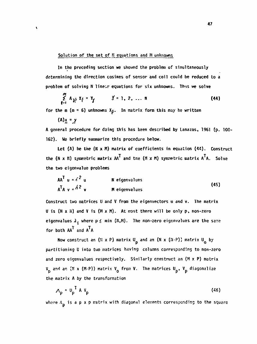
Solution of t h e se t of - ?I eguations and M unknams

In the preceding section we showed the problem of sinultaneously

determining the direction cosines of sensor and coil could be reduced Lo a

problem of solving N l i n e ~ r equations for six unknowns. Thtts we solve

for the m (in = 6) unknowns X?. In matrix form t h i s nay be written

(A)!! =_y A general procedcre for doins this has been Oescri bed by Lanazos, 1961 (p. 100-

162). k k briefly summarize this procedure below.

Let (A) be the (!I x M) matrix of coefficients in equation (44)- Ccnstruct T T the (N x ti) symetric matrix AA and tne (M x t4) symetric natrix A A. Solve

the two eigenvalue problems

N eigenval ues

M ei genval ues

Construct two matrices U and V from the eigenvectors u and v. The matrix

U is ( N x N) and V i s (N x M). A t most there will be only p , non-zero

eigenvalu-~s ,Ii where p < min (N,M). The non-zero eig~nvaluts are the sans

for both AAT and AT^ Now construct an (!I x P ) matrix U and an (N x ( i l -P ) ) matrix Uo by

P pzrti tioning U into trm natrices hav ing colums corresponding to non-zero

and zero eigenvalues respectively. Similarly construct an ( M x P) matrix

V 2nd ar! {A x (M-P)) matrix Vo from V. The matrices U V diagonalize P P' P

the matrix A by the transformation

T Ap = Up A vp

where 4 i s a p x p matrix with diagonal elements correspond in^ to t h e squzrc P

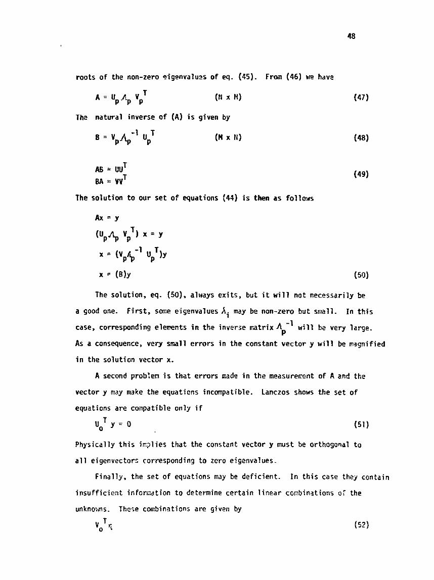
roots o f the non-zero sigenvaluss o f eq. (45). Frax (46) we havc

The natural inverse of (A) i s given by

The solution t o our set o f equations (44) i s then as fol lows

The solution, eq. (50), always exits, but i t w i l l not necessarily be

a good one. F i rs t , sme ei~envalues Ai may be non-zero btit small. I n t h i s

case, corresponding elements i n the inverse ~ a t r i x A " w i l l k very large. P

As a consequence, very small errors i n the constant vector y w i l l be nagnif ied

i n the solut ion vector x.

A second prob?ern i s tha t errors nade i n the measurerent o f A and the

vector y may make the equaticns incompatible. Lanczos shows the set o f

equations are coinpatible only i f

Physically t h i s ia2 l ies that the constant vector y must be or thogo~al t o

a l l eigenvectors corresponding t o zero eigenvalues-

Finally, the set of equations may be deficient. I n t h i s case they contain

insuf f ic ient in fomat ion t o determine certain l inear co~bin3tions o r the

unknolrns. These combinations are given by

where V is the matrix of zero eigenvectors from the matr ix V and r, is an 0

arbitrary column vector.

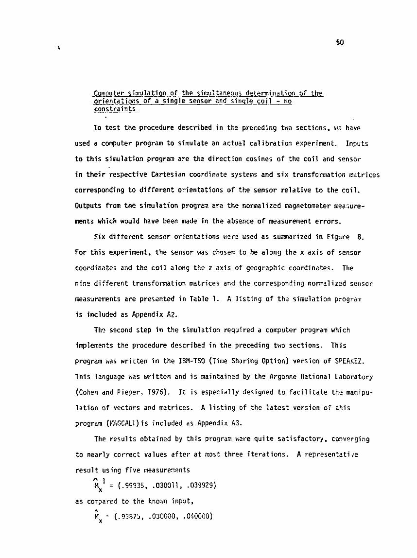
Comwtcr simulation of the simultaneous determination of the --- ------ --..------..-.----

orientations of a single sensor and sinqle coi 1 - IIO --- constraints-

To t e s t the procedure described in the preceding two sections, w2 have

used a computer program to simulate an actual calibration experiment. Inputs

t o t h i s simulation program are thc direction cosines of the coil and sensor

i n t he i r respective Cartesian coordinate sysieins and s ix transformation matrices

corresponding to different orientations o f the sensor relative t o the coi 1.

Outputs from the s i ~ u l a t i o n progrzz zrz the normalized nagn2tometer measure-

ments which would have been made in the absrnce of measurenient errors.

S i x different sensor orientations wert used as su~marized i n Figure 8.

For t h i s expe r i~en t , the sensor was chosen to be along t h s x axis of sensor

coordinates and the coil along the z xis of geographic coordinates. The

n i n s different transformation matrices and the corresponding nomalized sensor

neasurements are presented i n Table 1. A l i s t ing of the simulation prograiri

is included as Appendix A2.

Thc second step i n the simulation required a computer program which

implenents the procedure described i n the preceding two sections. This

program was written in the IBM-TSO (Time Sharing Option) version of SPEAKEZ.

This language was writien and i s maintained by thz Argonne National Laboratory

(Cohen and Pieper- 1976). I t i s especially designed to f a c i l i t a t e the manipu-

lation o f vectors and matrices. A l i s t i ng o f the l a t e s t version of th is

progrcm (IfAGCALl ) i s included as Append i x A3.

The resul ts obtained by th i s program w2re quite sat isfactory, converging

to nearly correct values a f t e r a t ~ o s t three i terat ions. A representati fe

resul t using five msasurezents

as cocpared to the kno:m i n p 3 t , A

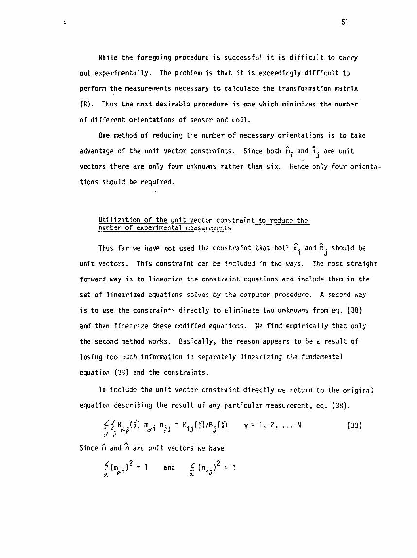
While the foregoing procedure i s successful i t i s di fficul t to carry

out experimentally. The prsblem i s that i t i s exceedingly d i f f i cu l t t o

perform the measurements necessary t o calculate the transformation rcatrix

( R ) Thus the most d e s i r a b l ~ procedure is one which minimizes the numb9r

of different orientations of sensor and coil .

One method of reducing the number of necessary orientations i s to take

advantage of the unit vector constraints. Since both f i and a. are u n i t 3

vectors there are only four unknowns rather than six. Hmce only four orienta-

tions should be required.

Utilization of the unit vector constraint t o reduce the nunber of experircental reasure~ents

Thus f a r we have not used t h ? constraint that both Ei and d - should be J

unit vectors. This constraint can be included i n two ways. The most s t ra ight

forward way i s t o l inearize the constraint equations and include them i n the

set of linearized equations solved by the computer procedure. A second way

i s t o use the constrainc. directly to eliminate two unknowns from eq. (38)

and then linearize these modified equations. iie find empirically that only

the second method works. Basically, the reason appears to t 2 a resul t of

losing too much information i n separately linearizing t h 2 funciarental

equation (38) and the constraints.

To include the unit vector constraint direct ly \$e rcturn to the original

equation describing the rtsul t o i any particular measurezent, eq. (38).

Since :I and ?I are unit vectors Re have

. .'

we may solve these fo r t hc diagonal elements

wh i l e these can be s u b s t i t u t e d d i r e c t l y i n eq. (38) i t i s no t necessary t o

do so. Instead, we t r e a t eq. (38) as b-Fore as a f u n c t i o n o f s i x var iables,

i .e.

but u t i l i z e the r u l e s fo r imp1 i c i t d i f f e r e n t i a t i o n t o evaluate t h e de r i va t i ves

o f the diagonal elements. Thus,

where -

I s o l a t i n g t h e diagonal element i n each SUFI give;

From equations (54 & 55) t h e t o t a l de r i va t i ves o f t h e diagonal elements are

Subs t i t u t i ng i n eq. (55) gives

Since 4 takes on on l y two values i n each sensor we have c l e a r l y reduced the

number o f unknowns from s i x t o four . The remaining two unknowns are defined

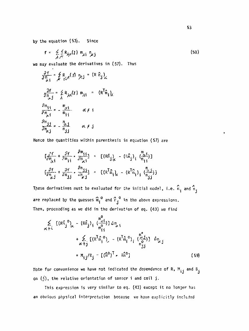
by t h e equat ion ( 53j. Since

f = t 4 ~ ~ ) , ( 1 ) mAi >j A f i

we niay evaluate the de r i va t i ves i n (57). Thus

Hence the q u a n t i t i e s w i t h i n parenthesis i n eqcat ion (57) are

Ir A These d e r i v a t i v e s must b2 evaluated f o r the i n i t i a l model, i.e. r,. and n

1 j

are replaced by the guesses GiO 2nd $ O i n the above expressions. j

Then, p r o c w d i n g as we d id i n the d e r i v a t i o n o f eq. (43) we f i n d

. -

T n 0 no

+ t. [(R mi )*, - ( ~ ~ 4 ~ ~ ) ~ (-$)I f i $ j 4[$3 11 j j

Note f o r convenience we have n o t i nd i ca ted the dependance o f R, 4 and B 3 -

on (i), t he r e l a t i v e o r i e n t a t i o n o f sensor i and c o i l j.

This expression i s ve ry s i m i l a r t o eq. (43) except i t no longer has

an obvious physical i n t e r p r c t a t i o n because we have expl i c i t l y i n c l ~ d ~ d

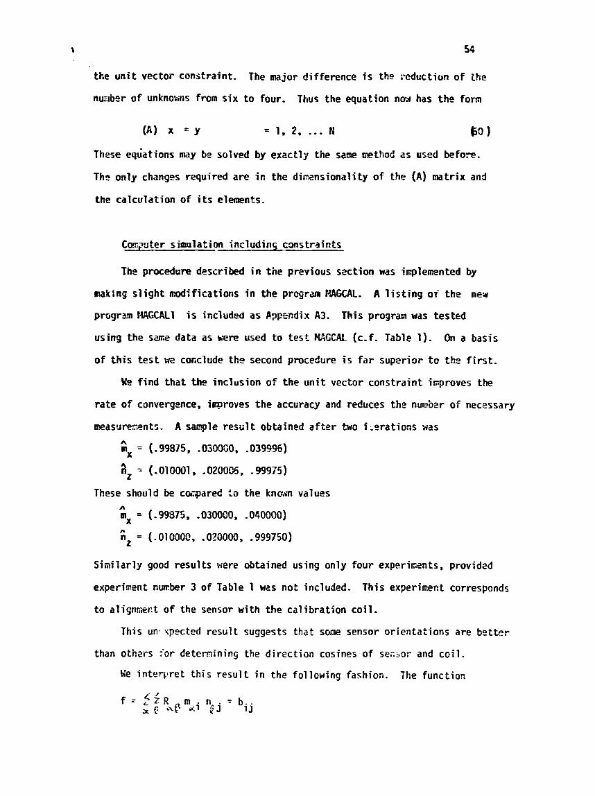
the u n i t vector constraint. The major difference i s the reduction o f the

nusbor o f unknowns f rom s i x t o four. Thus the equation nu.* has the form

(A) x = Y = 1, 2, ... x 60 1

These equ'ations m y be solved by exactly the same mthod as used before.

The only changes required are i n the dintnsional i ty of the (A) matrix and

the calculation of i t s elements.

Coqster simulation includincj cmstra ints

The procedure described i n the previous section was iuplewnted by

making s l i gh t d i f i c a t i o n s i n the prwjram ~4#%AL- A l i s t i n g o i the new

progrm !iiGCPiLl i s included as Rpp~ndix A3. This program was tested

using the sac. data as were used t o tes t M r j C A t (c-f, Table 1). On a basis

o f t h i s t es t we cocclude the second procedure i s f a r sup2rior t o the f i r s t .

We f i n d that tho inclusion o f the u n i t vector constraint improves the

rate o f convergence, i q roves the accuracy and reduces the nmbgr o f necessary

neasrrterents. A s a q l e r e s ~ l t obtained a f t e r two i -?rat ions Has A

"x = ( -99875, . 0300G0, -039995)

4

"2 = (- 01 0001 , .020095, -99975)

These should be cacared t o the knmn values A

mx = (. 99875, -030f0, .040000) n

"z = ( -01 0000, .020000, -999750)

Sini l a r l y good resul ts were obtained using only four experir ints , providzd

experinent n u r k r 3 of Table 1 wzs not included. This experiment corresponds

t o a1ignrer.t o f the sensor with the cal ibrat ion co i l .

This UP* upected resul t suggests that sme sensor orientations are bz t te r

than others for determinins the direct ion cosines of sezsor and co i l .

Ue in ter j l rc t th is resu l t i n the following fashion. The function

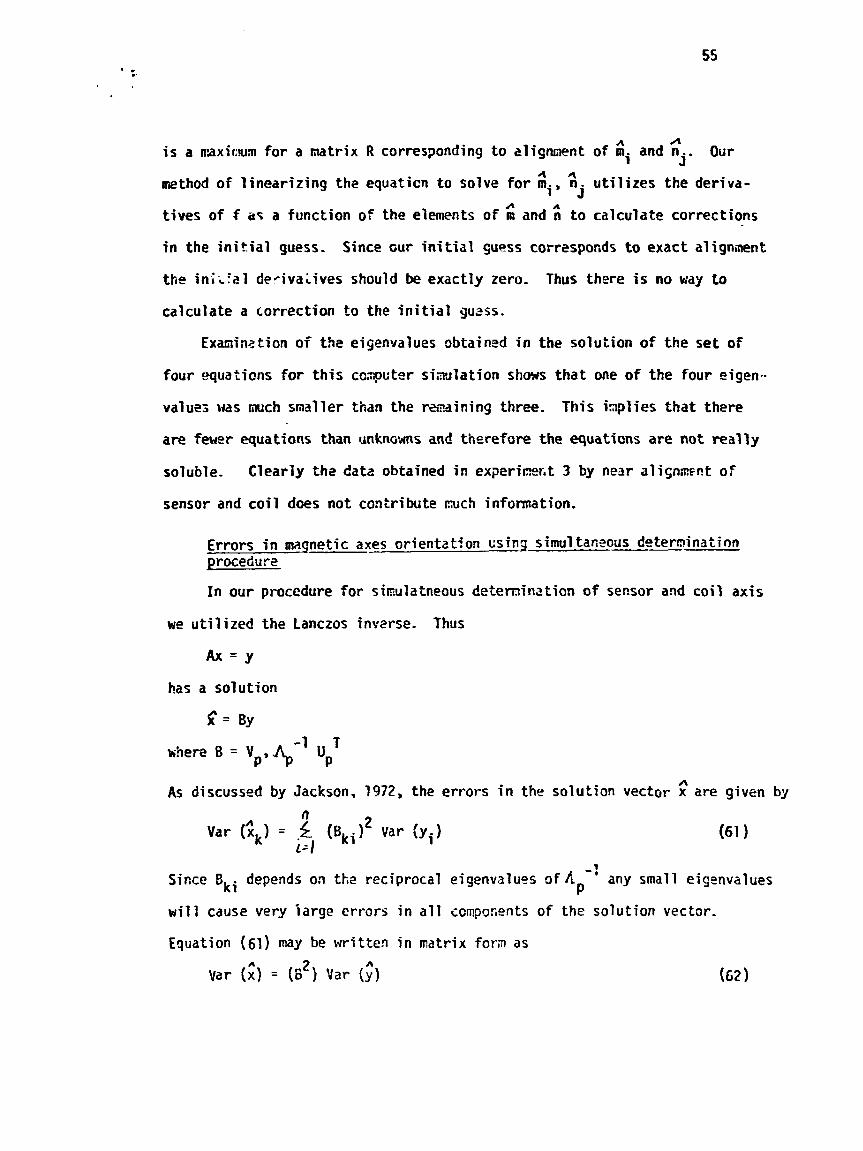
A i s a n a x i r ~ n f o r a m t r i x R c o r r e s p o n d i n g t o a l i p m n t o f $ . a n d n Our

1 j - 4 4 nethod o f linearizing t h e equaticn to solve for mi, n. ut i l izes the deriva-

A J

t ives of f a% a function of the elements of m and An t o calculate corrections

i n the i n i t i a l guess, Since cur i n i t i a l guess corresponds t o exact aligntnent

t h e in-icral decivaLives should be exactly zero. Thus there is no way t o

calculate a correction t o t h e i n i t i a l 9uass.

Exanin2tion o f t b e eigenvalues obtaintd in t h e solution of t h e set of

four equations for t h i s c ~ q u t e r siimlation shows tha t one of t h e four eigen-

valuts was mch smaller than the rmaining t h r e e . Th i s izplies tha t there

are f e e r equations than unknc8ms and tierefore t h e equations are not real ly

soluble. Clearly the data obtained i n expericerat 3 by near a l i snm~nt of

sensor and coil does not contribute nuch information,

Errors i n maqnetic axes orientation csinq simultansous determination procedure

In our procedure for siaulaineous detemination of sensor and co i l axis

we util ized the Lanczos inv2rse. Thus

has a solution

c = By

A As discussed by Jackson, 1972, the errors i n the solution vector x are given by

- ? Since Bki depends on the reciprocal eigenvalues o f J'L any small eigenvalues P will cause very iarge errors i n a l l components of t h e solution vector.

Equation (61) may be written in matrix for3 as

var ( = (El2) var (62)

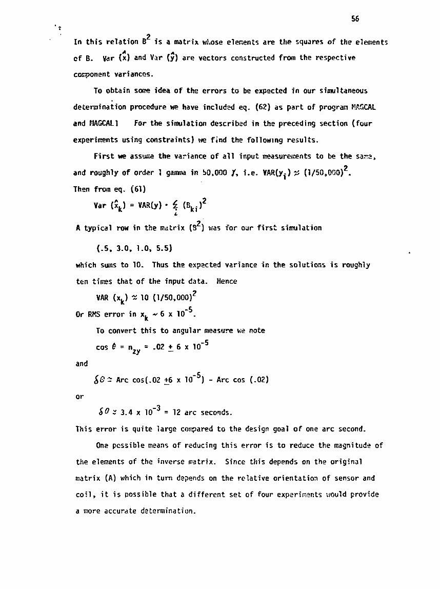
56 - 2

In t h i s relation 8 i s a matrix wf,ose e lemnts are t h e squ~res of t h e elements A

cf 6. Var (x) and Var (?) are vectors constructed from the respective

cocponent variances.

To obtain sax idea of the errors to be expected i n our simultaneous

detemination procedure we have inc ludd eq. (62) as par t of program ?NSCAL

and klAGCAL1 For the simulation describzd in the preceding section (four

experimnts using constraints) we find the fol lowlng results.

F i r s t we asswr2 the variance of a l l input measureiients to be the s a r p ,

2 and roughly of order : gaorna i n 50,000 1, e VAR(yi) "r (1/50,000) . Then fma eq. (61)

2 A typical r o w i n the s a t r i x (3 ) for oar f i r s t simulation

( -5 , 3.0, 1-0, 5.5)

which sums to 10, Thus the expzcted variance i n t h e solutions is roughly

ten t ines that of the input data. Hence

VAR (xt) Z 10 (1/50,000)*

Or RW er ror in xk I. 6 x IO-'.

To convert t h i s t o angular measu?-e te note

cos 6 = n = -02 + 6 x ZY -

and

& @ 2 Arc cos(.02 - +6 x - Arc cos (-02)

or

60 2 3.4 x 1d3 = 12 arc secolds.

T h i s e r ror i s quite large coqared t o the design goal of one arc second.

One possible means of reducing t h i s error is to reduce the magnitude of

the elements of the inverse ~ a t r i x . Since this depends on the original

matrix (A) which in t u r n depends on the relative orientation of sensor and

co i l , i t i s possible that a different set o f four expe r i~2n t s would provide

a more accurate de tcmination.

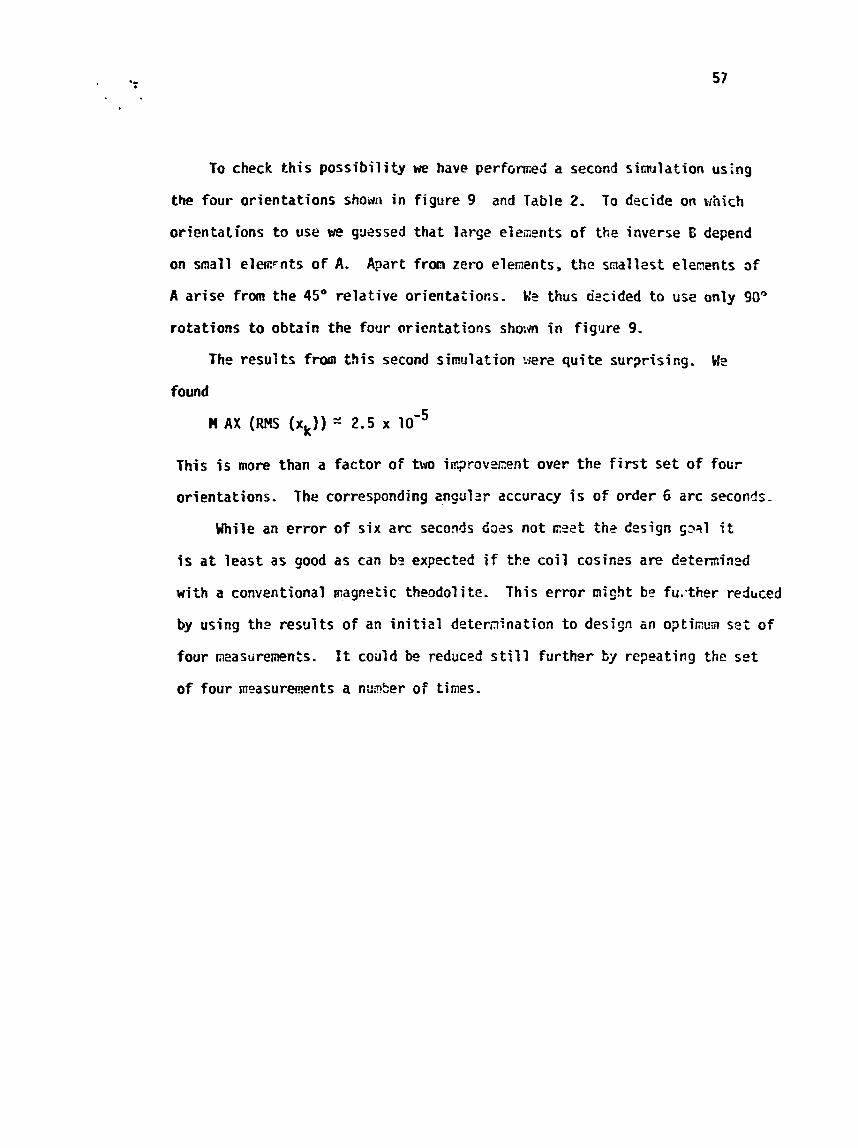
To check this possibility we have perfornied a second simllation using

the four orientations shoi~rl in figure 9 and Table 2, To decide on which

orientations t o use goessed that large elemnts of the inverse B depend

on small e l twnts of A. Apart fron zero elments, the snall2st elensnts a f

A arise from t h e 45O relative orientations. b!? thus dttided to use only 90"

rotations to obtain the four orientations sham i n figure 9.

The results fron this second simulation !+ere quite surprising, Me

found

n AX (RMS fxk)) = 2.5

This i s more than a factor of trqo iix?ravemnt over the f i r s t se t of four

orientations. The corresponding anculsr accuracy i s of order 6 arc seconds-

Hhile an error of six arc seconds docs not rr,?et t h e design ~ 3 1 1 i t

i s a t least a s good as can b? expected i f t h e coil cosines are detem.in2d

w i t h a conventional ~agne t ic theodolite. This error misfit b? fu:ther redirced

by using th,o resg'lts of an ini t ial deternination to design G n o?tinum set of

four m2asurercen;s. I t could be reduced s t i l l further by repeating the sot

of four measure~ents a no~5er of tines.

Calibration of Three Sensors Usinq Three Calibration Coils

In the preceding section we shewed hew a single sensor corlld

be calibrated using only one coil. This procedure regtiires a sufficient

number of relative oriantations of the sensor and coil t o define a1 l

of the unknowns. In t h i s section ~e show how the use of t h r e e coils nzkes i t

possible t~ calibrate three sensors with the sane number of orientations,

Let u s assume as k fore , that for each sensor orientation we carry out

three masurments. Each masurecent is the vector output of t h e sensor

assembly for a given calibration field- The expected fields for this set of

three weasure~ents my be written

where B and B, are S x 3 matrices x i th colu~n corresponding t o the three Gl

neasured and calibration fields resp2ctivtly This may be ~;rf cten

where b = (B)(,) is the "nonnalizedn observation matrix.

To linearize this set of equations for p and I-I we assuze an approxi~ate

mode: is kncn, i .e. p = and n = g. Ir 0

t 4 ~ then write v and Q as small pertur-

bations about this known model, t h u s

P = Yo + 6~

Q = no + 6r!

Substituting i n equation (63) we f i n d

T irihere we O!-op the second ordsr term bu 67 which we a s s m e t o be very sc211.

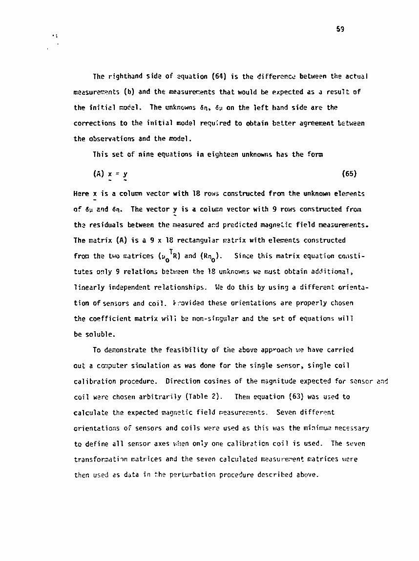
The righthand s ide of equation (64) is the di Fferefice between the actual

m ~ z s u r s s ~ n i s (b) and the measurw.ens tha t would be expected as a resul t of

the i n i t i a l noc'zl. The cnknowns 6s, 63 on the l e f t hand side are the

corrections t o the i r ~ i t i 31 model rcgui red t o obtain be t te r agreetent between

t h e observations and t h e codel.

This set of nine equations in eighteen unknowns has the form

(A) x = y - - Htre x is a column vector with 18 ro:+s constructed from the unknown elwents - of 6;1 2nd 6s. The vector y is a c o l u ~ n vector with 9 ro:s constructed f r m - thz residuals between the measured acrf predicted magne',ic f i e ld neasuments.

The matrix (A) is a 9 x 18 rectangular ea t r ix ui t h e l e ~ e n t s constructed

T f r m t h e two mt r i ces (u0 R) and (Hso). Since th is matrix equation caiisti-

t z tes only 9 relztion5 bzt?.tzen the 18 unkfi~wcs w2 ~ u s t obtain additional,

l i n e ~ r l y indspendent relationships. \+e do th is by using a different orienta-

tion of sensors and coi l . t:-3viG?cl these orientations a re properly chosen

the coefficient matrix wili be non-s:ng~lar and the s e t of equations wil l

be soluble.

To dczonstrate the feas ib i l i ty of the above approach we have carried

out a cc-nputer s i n ~ l a t i o n as was done for the single sensor, single coil

calibration procedure. Direction cosines of the n~gni tude expected for senscr aad

coil w w t ? chosen arb i t ra r i ly (Table 2). Then equaticn (63) was i i~ed to

calculate the expected magnetic f ie ld ~:ossureaents. Seven di f ferent

orientztions oT sensors and coi l s were uscld a s th is was the mi2inul;l necessary

to define a l l sensor axes uiten only one calibrzticn co i l is used. The seven

trjnsfomati?n natrices and the seven calculated masurepent ~ a t r i c e s were

then used 2s data in the perturbation procedure described above.

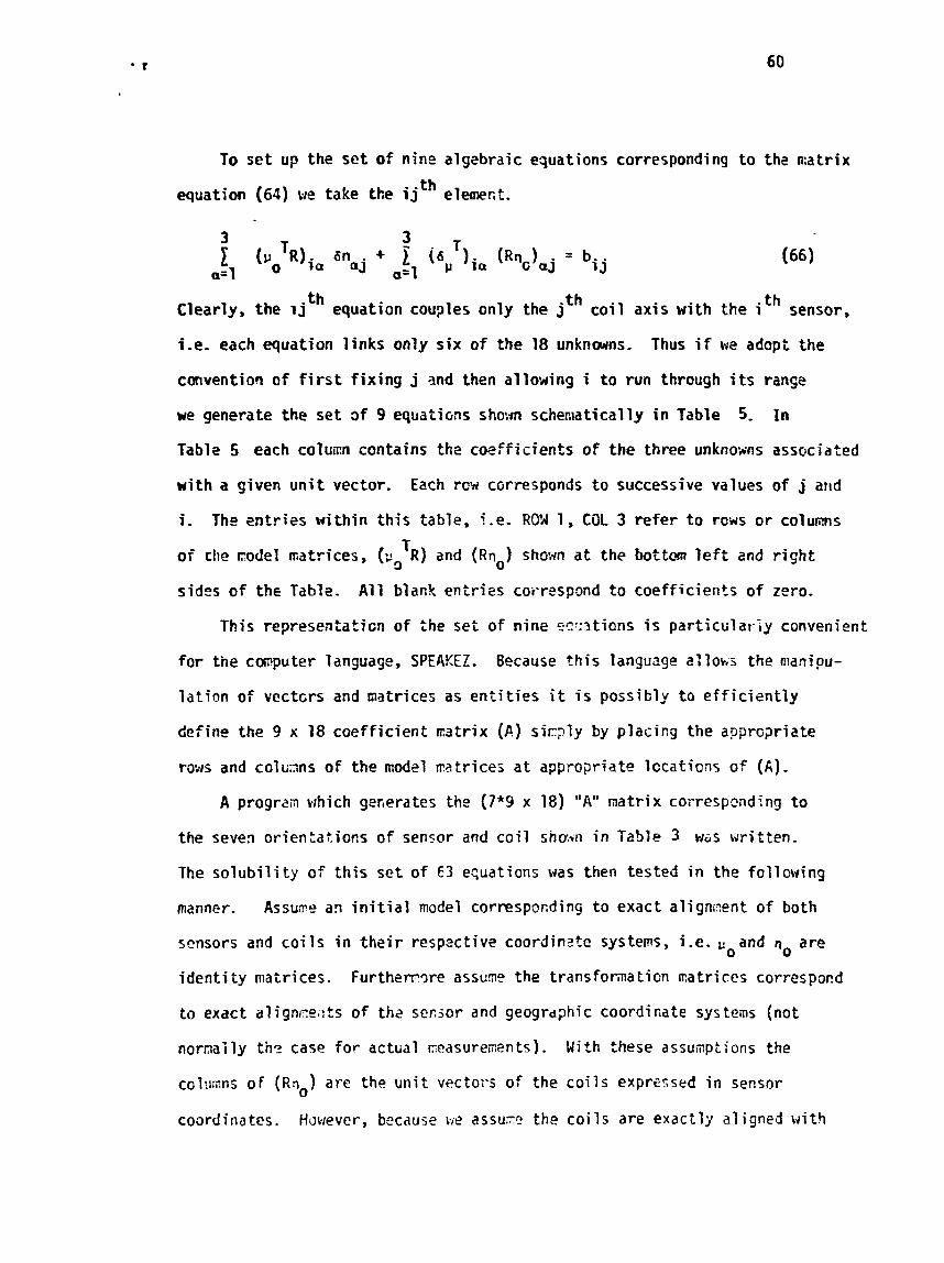
To set up the set of nine algebraic equations corresponding to t h z natr ix

equation (64) I;E take the ijth e1mer.t.

Clearly, the I jth equation couples only t h e jth coil axis w i t h the i th sensor,

i - e . each equation links only six of the 18 unknw.+ns. Thus if ~2 a d ~ p i the

convention of f i r s t fixing j and then allouing i to r u n through i t s range

we generate the s e t 3f 9 equaticns shoxn schematically i n Table 5. In

Table 5 each c o l u ~ n contains the coefficients of t h e three unknowns assciciated

with a given u n i t vector. Each rm corresponds to successive values of j and

i. The sn t r ies within this table, i.e. RON 1 , COL 3 refer t o rows o r c o l u ~ n s

T of the sodel catr ices , (so R) and ( R l o ) shown a t the bottm l e f t and r i ~ h t

sides of t h ~ Table. All blank entr ies coi-rsspond t o coefficients of zero-

This representaticn of :he set of nine ec,:3tians is particulat-;y convenient

f o r tne computer language, SPEAREZ. Because th i s language a: toirts the manipu-

lation of v e c t ~ r s and ~ a t r i c e s as en t i t i e s i t i s possibly to e f f ic ien t ly

define t h e 9 x 18 coefficient tratrix (A) sic7ly by placing the apprcpia te

rcr.qs and co1w;nns of the model ~ a t r i c e s a t approprizto Iccaticar of ( A ) .

A progrsm which gerierates the (7*9 x 18) "A" nat r ix corresp2nding t o

the seven orientations of sensor and coi l snmn in Tablp 3 WGS written.

The solubi l i ty of th i s s e t of E3 equations was then tested in the fcllaving

manner. Assure an i n i t i a l model corresponding t o exact aligncent of both

sensors and coi l s i n the i r respactive coordinctc systems, i.e. I: and so are 0

identi t y matrices. Furtherr.ore assumo the transfoma tion ~ a t r i ces correspond

to exact align:e,~ts of ths secjor znd geographic coordinate systems (not

normai ly thc case for actual ceasurements) . M i t h these a s s u ~ p t ions the

co lu~ns o f (RQ ) are t h f ! u n i t vectors of the coi ls exprsssed in sensor 0

coordinatcs. Hilwever, because Vi? assuTe the coi Is are exactly .3l igned with

geographic coordinates the columns of (Rq0) are actually the unit vectors of

geographic coordinates as seen i n sensor coordinates. Similarly, rows of T T (r, R ) correspond to columns of (R uo), but by the same arguments as above

these are the unit vectors of sensor coordinates as seen i n geographic

coorc. lates. Using these facts we can immediately write down the elements

of the A matrix by inspection. To decide whether th is se t of

e~uat ions can be solved we take the deteminant. If this i s non-zero the

matrix i s non-singular and the equations soluble.

For the A matrix based on the seven orientations of Table 3 SPEAKEZ

wthods sho;~ed the deteminant was zero. Thus the equations were insoluble.

Our interpretation of t h i s result is as follows- The seven orientations of

table 3 weredeliberately chosen to produce a specific set of four oriefita-

tions of each sensor relative to one coil. These sets of four orientztions

were chosen so that the four unknoams associated w i t h oae coil and one sensor

could be determined. Only four unkacwns xere present because the u n i t vector

constraints were used to eliminate two of the six unkno:~ns.

This argument leads us to the conclusion that a t least several

additional orientations would be required to solve fo r the 18 unknowns by

the above method, Because of the experirna~tal diff icult ies associated with

the m2asurement of the R rriatrix we rule this out a s a viable procedure.

Consequently, we extend the foregoing procedure to make use of the six unit

vector constraints.

The constraint equztions may be written d.

Solving f o r t ho diagorial elenents we hav2 for coluiitns of (n)

In our perturbation approxirration

So that the diagonal elements become

Expanding the square and dropping second order terns gives

But

so that

Because the second term within the brackets i s much smaller than one we

have

or finally

In an analogous fashion

To include these constraints i n a modif ied A mat r i x we note the fol lowing.

The two constraints may be wr i t t en i n the form

Now mu l t i p l y the f i r s t equation by the co lum o f the A matr ix corresponding

t o the unknown bn jj - S im i la r l y mu1 t i p l y the second equation by the column

o f A corresponding t o timi i. Then, add the two equations obtain ing

F ina l ly , add t h i s equation the i jth equation previously obtained wi thout

using constraints. (eq. (66)).

When t h i s procedure i s ca r r ied ou t e x p l i c i t l y i t can be seen tha t i t i s

exact ly equivalent t o subs t i tu t ing the const ra in t equations f o r the diagonal

elements and then rearranging terns. Thus t o modify the A matr ix sham i n

Table 5 we must construct 2 (9 x 18) M matr ix w i t h the elecents shown i n

Table 6 Then t h i s matr ix (N) must bg subtracted from the matr ix (A).

Subtract ion w i l l introduce zeros i n the colunns o f the modif ied A matr ix

corresponding t o the diagonal elements o f the unknown n;atrices (?i9), (6n).

I f we now el iminate a l l comumns o f the modif ied A n a t r i x corre,?onding t o

these diagonal elewnts we w i l l obtain a new set o f equations o f the f o m

where now x' i s a column vector w i th 12 unknowns taken from the o f f diagonal - elements of (so), (6~). y i s a 9 row column vector o f residuals between - observations and predict ions as previously defined. The n a t r i x (AA) i s a

(9 x 12) rectangular matrix obtained as described above.

A SPEAKEZ program "EQUATS" was written to implement th i s procedure.

A l i s t i ng of this program is included as Appendix As. In the i n i t i a l text of

th i s program a l l seven orientations of table 3 were used t9 construct

a (63 x 12) matrix (AA). The determinant of t h i s matrix was found to be

non-zero for the particular simulation used. Consequently two addi t i ~ n a l

programs were written to solve fo r the direction cosines in. an i te ra t ive

fashion.

Program "SOLEQU" ( l i s t ing also included i n Appendix A5), u t i l i zes a

SPEAKEZ linkule (similar to subroutine) to solve the s e t of equations d2fined

by the matrix (AA) and thz vector y. This linkule u t i l i zes the singular - value decomposition procedure of Lanzcos described ear l ier .

Because t h i s linkule is written t o minimize time and storage requirements

i t does n o t provide as much information as our own implementation of t h i s

procedure embodied i n pr-rarn MAGCAL and PIGCAL 1 (See Appendix A3) .

However, bec~use our implementation u t i l izes too much storaqe w 2 were unable

t o use i t to solve the s e t of 63 equations.

A second program "EIAINPO" was written to itxplement the i te ra t ive perturba-

tion procedure our method of simltaneous solution i s based on. This pro3rarn

in i t i a t i zes the calculation f i r s t reading i n the measure~ents and transforr~jiio: 0

matrices, and then reading a f i r s t guess of the unknowns, (q ) and (uO).

Normally w2 assune these are identity matrices since these a re the design

goals fo r both sensors and coi 1 s. The program then ca l l s program EQgATS.

As i t s f i r s t step program EQUATS increments (pO) and (no) using previously

calculated corrections (6u) and (6n). ( In i t i a l ly these are zero). EQUATS

then uses the constraint conditions to calculate the diagonal elements of the

modified matrices (PO + 6 ~ ) and (no + 6n). I t then proceeds to generate

the matrix ( A A ) and the vector y. Control i s passed to program f4AINPO hhich -

6 5 I

- 9 . t ca l l s SOtEQU to solve the se t of equations for the vector x. In i t s f ina l - step SOtEQU creates the correction matrices ( 6 ~ ) and ( b n ) froit1 elements of the

solution vector x. Control '- returned to program 'PlAINPO which loops back - t o cal l program EQUATS. This procedure is repeated the number of t ines

specific .during the in i t ia t iza t ion phase o f program MAINPO.

Results obtained with program MAINPO are comparable to those obtained

with the programs which were written to solve the case of one sensor and one

coi l . For example, the second corrected model was equal t o the model used in

the simulztion program to better than the f i f t h decimal place.

To d~termine the m i n i m u m nunber of orientations required to carry out

a procedure wc progressively reduced the number of different orientations

ingut t o program MAINPO. When th i s nunber was less than four, the deterninant

became zero and we were unab le t o obtain a correct solution t o the proolen.

Although we have only examined t h e case corresponding t o the first four

- ;entations of table 3, we belieye t h a t any four orientations satisfying the

fo1;:xing c r i t e r i a would be sufficient t o define the 18 direction cosines of (p )

and (n) using our procedure. These cr i te r ia are the same as was found f o r

calibrating a single sensor with a single coil: (1) there must be 4 different

orientations of the sensor and the co i l , ( 2 ) d i rect alignsent of th. sensor and

coil provides no useful infornation, (3) rotations of 90" from the ini t i 2 1

position ggnerate satisfactory orientation provided one rotation brings the sensor

axis i n i t i a l l y transverst t o both coif and sensor parallel t o calibration co i 7 .

In surmnary, our procedure for calibrating the direction cosines of a

three axis sensor assembly using a three axis Helmholtz coil systcni i s the

following. Attach an optical cub2 to the sensor assembly. Place the sensor

assembly in a f ixture that al1o;vs 90' rotations about two orthogonal axes

and which does not allow the center of the cube to t ranslate during rotation.

Begin with an alignment which places the x ' , y ' , z ' axes of the sensor, i . e .

of the o?tical cube, in near coincidence with the x , y, z axes of the c o i l ,

i .e . of geographic coordinates (c.f . Figure 9 ). Level the f ixture u s i n g

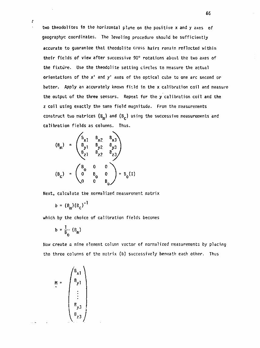
6 €

two theodolites in the horizontal plane on the positive x and y axes of

geographyc coordinates. The level i n g procedure should be suff ic ient ly

accurate t o guarantee that theodol i te cross hairs remain reflected w i thin

their f ie lds o f view a f t e r successive 90" rotations about the two axes of

the fixture. Use the theodolite set t ing c i rc les t o moasure the actual

orientations of the x ' and y' axes of the optical cube to one arc second or

better. Apply an accurately known fi5ld i n the x calibration coil acd msasure

the output of the three sensors. Repeat for the y calibration coil and the

2 coil using exactly the sam? f i e ld magnitude. From the ~easurerr;ents

construct two matrices (B,) and (Bc) using the successive measurements and

calibration f ie lds as columns. Thus.

Next, calculate the normalized seasureoent matrix

which by the choice of calibration f i e l d s beconies

Now create i~ nine element column vector of normalized neasurenents by placing

the three columns o f the matrix (b) successive1y beneath each other. Thus

Finally, using the orientation angles d2terminrd by the theodolites construct

the transformation matrix ( R ) from georjraphic to sensor coot-d ina tes.

The ( 3 x . 3 ) rotation n~atr ic (R) and the nine elen~ent colurnrl vector

M are the data to be i n p u t t o the sirngltaneous equation solving program f:A!l:PO. "

Having completed the measurements for the f i r s t orientation we rotate

the sensor assembly + 90° about i t s z cxis (azimuth axis of f ixture) . The

actual orientations of two sensor axes of the sensor assembly are determined

by the x and y theodolites as before. Ke then repeat the previous sequence

of three cal i brati on f ie lds and corresponding ~easureo:ents. A matrix !'

and a vector M calculated as above form the second set of input data ' , p . . - MAINPO.

For the third orientation of f igure 9 we rotate an additional + 9iI0

about the azimuth a x i s of the fixture and ob ta in rxeasurenents a s before.

Finally, the fourth orientation is obtained by a 90" rotation about t h ?

elevation hxis o f the fixture. This brings the top of the optical cube dowi

t o a position where i t may be viewed by the y theodolite.

After a1 1 data have been properly en tcr-ed into program MAIFIPO, the prosram

requests an i n i t i a l guess for the s l t r i c e s ( v ) and (Q) defining t h ~ direction

cosines o f the sensors i n sensor coordin3tes and o f the coi ls i n geographic

coordinates. I f no prior information i s available these are assi!neri t o be

identity matrices. The program then proceeds through several iterat5cqs

obtaining a f ina l , l eas t square determinatian of the best f i t of the dit-cciion

cosines of sensors and coi ls to the input data.

Recons:enda t i ons ---

The high absolute accuracy desired for t h e MAGSAT magnetoae ter req2i res

accurate czl i bra tion equipir;~n t and sorle n2;q proccdurcs. Kc recor-can4 acqui -, i t i c n

To make En accurate determination of sensor direct ion cosines, the

calibration coi 1 direction cosines must a l so be deternined accurately. This

can be done in trm ways.

1 ) Y i t b a magnetic theodolite which would need t o be purchased

2) Simlianeously as tho sensor cosines a r e determined

In our report we choose t h e simultaneous d2temination procedure, We

s h w tha t t h i s technique shculd be able t o provide accuracy of order 5-10 a rc

seconds. This eccuracy is canparable t o that of eas i ly acquired magnetic

theodol i tes. To significantly improve t h i s accuracy narld requi i-e repcaced

measurmeat of the direction cosines. :his procedure requires focr reorien-

ta t ions of t h e sensor assembly. For each orientation both theodolites must

be read and 3 ser ies of three calibration fields applied and t h e ma~neiameter

v t p u t recorded.

Ke recomend t h a t t h i s procedure b2 autorated and placed under the

control of a minicmputer. This wozld require tha t the rotation f ixture have

motor control of each axis- Addi tionat ly , the theodolites should have dig i ta l

readouts.

I f w2 accept 10 a rc seconds as the obtainable accuracy of t h e direction

cosines of the sensors, then t h e absolute accurzcy of the magnetunster cacnot

be better than - + 2 gaama. Howzver, individual sensor errors w i l l a l so be

about - + 1 g a m , so we expect the f ina l accuracy to be about 5 3 gairma.

Siqnificantly iirtproving t h i s accuracy appears t o involve very labor i n tsnsfve

calibration procedures.

of the following equipment:

1 ) Two optical theodolites of one arc second accuracy

2) Six digi t digital voltmeter

3) Two precision levels of one arc second accruacy

4) Smooth, nun-magnetic t e s t table of granite or glass

5) Brass fixture for rotating sensor assmbly about horizontal and

vertical axes with precision of order one minute

6) Miniccmputer controller and data logger with vide0 display keyboard

en try

Several modifications of t h e existing faci l i ty a lso appsar to be

regui red. These include:

1) Separate pi l lars sunk to bedrack on the h'orth and East calibration

coil axes. These will hold t h e two th,podolites.

2) Two optically f l a t ports a t r i g h t angles t o each other it? the thermal

snroud to monitor chan~es i n sensor orientation as a function of

tenperarure.

One ritajor problem likely to be encountered i n the calibration procedures

i s d i ~ i t i z i n g the magnetmeter output w i t h sufficient precision. If a 16 bi t

Analog to Digital Converter i c used for the +63K to -64K gam2 dynanic ranse

the least significant b i t will corres;lond to 2 gamna- T h i s iincertainty

of - + 7 gama l i d ts ths accuracy of the calibrations to an unacceptaboe level - Two solutions for t h i s problem are possible:

1) Use a d3ta logger to make a largz number of s a ~ p l e s aild average

to higher precisior,. (This wrks only Sf the faci t i ty noise i s larcje.;

2) Use AC signals rather than OC signals as the calibration fields.

If faci l i ty n ~ i s e i s low, small signals must be pressnt i n calibration

axes orthosonal t o train calibration fields. Use least square sine wave

f i t s to deternine AC signzl amp7 i tude; precisely.

Acknowl edganents

We would like to thank Dr. H. Farthing of Goddard Space Flight Center

and Hr. F. Hobley of t h e Johns Hopkins Applied Physics Laboratory for

helpful cements on magnetowter calibration. Also, we thank Mr. E. Seiifer

of knes Research Laboratory and N r - C. A. Harris of Goddard Space F l ight

Center f o r a l lor ing us t o v i s i t t he i r respective r a g n e t m t e r calibration

f ac i l i t i e s . IJ2 are grateful t o O r - 0. -lackson of UCLA fo r his suggestiocs

ccncerning the solution of s i m l t z n e c ~ s nanlinear equations. On? of us ,

Robert L. RcPhernn, would particularly like t o thank O r - D-J. h ' i l l ims

and t h e Epace Envirorunect Lzboratorl of ROAA in Boulder, Colorado fo r their

hospitali ty and support while cazpleting th i s mrk. This project has been

supported by NAS4 Contract HAS 5-23650 as par t of a design study f o r PIAGSM.

REFERENCES

Cain, J. t., b ~ n d table discussion o f reconnaendations for revis ion of the ICRF. -* EOS Trans. Amer. Ceophy. Union; 56(8):533, 1975- -

Harris, C- A,, Supplement 1 (1971) t o zmgnetic f i e l d rest ra ints fo r spacecraft system and subsystms. CSFC Rept. X-325-71-43S, Dec- 1971-

Hitdebrand, F. B., Introduction to I u i e r i c a l Aiialysis- Hc-Graw-Hill* Mu York, 1956.

HcLeod, H. C., Interim Report on a Propcsed Tr iax ia l D ig i ta l Fluxpate Hagnetmeter fo r NASA Appl i ca t ion Explorer ~ i s s ion% Dtsign-~tudy. IGPP Pub. Mo- 1643, Oct- 1976,

HcLegd, H. 6. and J. D- Heans, A Proposed D ig i ta l Fluxgate tlagneioneter fo r NASA Applications Explorer #ission: Results of Tests o f C r i t i c a l Elements, IGP? R e ~ t . f!n. 1675, Way 1977.

Schneider. Er ic J. and T k s s Kolany, The a~~tocc l l imator . Optical Spectra: Fourth Qtr.:24-28, 1967.

Stern, 0. P - , Enhanced errors i n models o f the c;lr1ir! geomagnetic f i e l d derived from scalar data- - EOS, Trans. ker. Geophy. Union, - 55!8j:j47; :975.

Yanagi I iara, K., H. Kawamura, Y. Sano ant! T . Kubk;, !Jew Standard Ragnet i c Observation System o f Kakioka (KASHHER). Geophys. Hagazine: - 3 5 ( 4 ) :217-281, 1973-

Figdre Czpt ions

1. Schenatic itlustration stzo.nin3 the a r ransc i in t o f c a l i b r a t i o n c o i l s

t es t t a b l e and theodoli tes. Theodolites and l e v e l s def ine the or tho~ona l , A A h

geographic cmrd inates X, Y, 2 - The d i rec t ion cosints o f the c a l i b r a t i o n

c o i l s i n seogcaphic cmrd inates are given by the nan-ort!ngonal u n i t A L A

vectors nX, ny, nZ,

2, Diagral;: showing a possible arrangsnant o f thre* r i n g core sensors

su?jmrtcd by a p l a s t i c c u k and topped by a s i lvered, o p t i c a l octagon.

Normd!s t o the faces o f tho, octagon estab l ish an orthogonal sensor

coordinate system, Thz d i rec t i on cosinzs o f the ragnet ic axes o f the

r i n g cores i n sensor coorti inates are given by the non-ortbgonal uai t

.L A a

veCiorS n xp '"v* "z-

3. A photograph o f an ear th inductor (or masnet ic theoclol i re) showing

the type o f f i x t u r e required f o r cal i b ra t i ng the angslar 0ri:niat ion of

a sensor tzagnatic axis i n sensor cmrdinates, As discussed i n t ex t the

r o ta t i f i g search c o i l i s replaced by a mun t i ng p l a t e t o ho ld sensor,

4. A schznaiic diagrsm shwing t h e modif ica t ions OF the ear th inductor

required t o obtain a magnztcmeter tes t f i x tu re .

5 . A schenatic i l l u s t r a t i o n showing hos~ angles 8'b 90° and $ 2 0*

are measured by thcodol i t e s t o determine absolute o r i en ta t i on o f norzzals

to the faces of an opt ica l octacjoa.

6. A f i x t u r e f o r a l i gn ing ind iv idua l sensors w i t h thz ca l i b r a i i o n f i e l d .

7. T y p i c a l noise spectren fo r a r i c s core f luxgatc sensor- Horizorrt~l

brackets a t top s5ow frequency band ~ a a s o r e d by an experim?nt o f g i ven

duration 2.74 sample rate. Dashed h~rizontsl :ine?s sh>..r quGntizaiion

n o i s e for 6 B = l y and 68 k l j 3 2 j .

8. S i x re la t ivs orientations of sensor and coi l used in f i r s t

computer sint.slation.

9. Four re la t ive orientat ions o f senssr and cqi i necessary for a

f u l l cal ibrat ion of three sensors and three coils,

Nor f h Theodolite v

t , ' ' - ' - '

1 . 1 ;/, .';; ' /,/-< ,:Q,q 4 vertical plane

n I ; Reflector nJ

Or thogonoi mit vectors cf geographic coordinaies

4- y Easf

i 9 Non-or fhogonol unit vectors of

; i z test coils Verficol

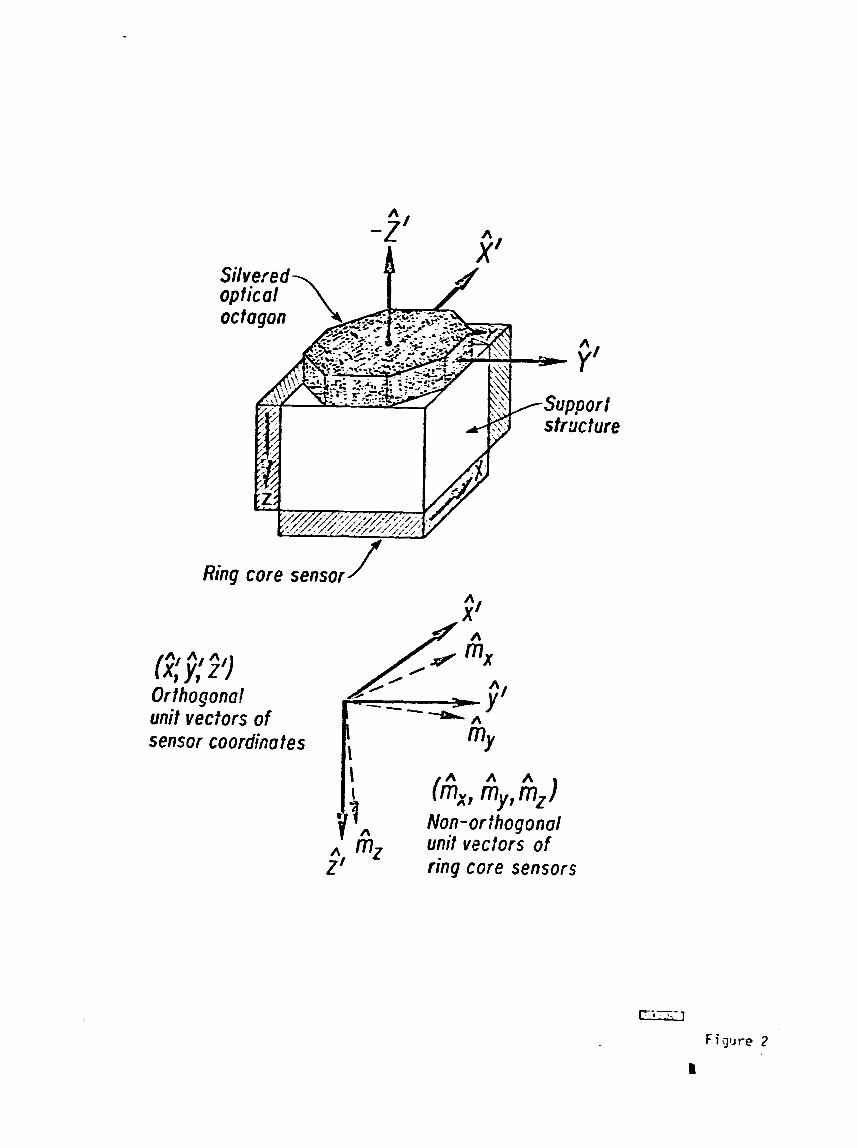
Ring core sensor1

"/ " / "/ (4 Y, z ) Orfhogonol unit vectors of sensor coordinates

A A

Non-orthogonal A m7 unit vectors o f f/ L ring core sensors

Figure ;,

O R M N f f i PAGE 16 OF POOR q ; A L m

Azimuth Axes

I screw

Light ray 7 - --- Sensor

L T f

Figure 4

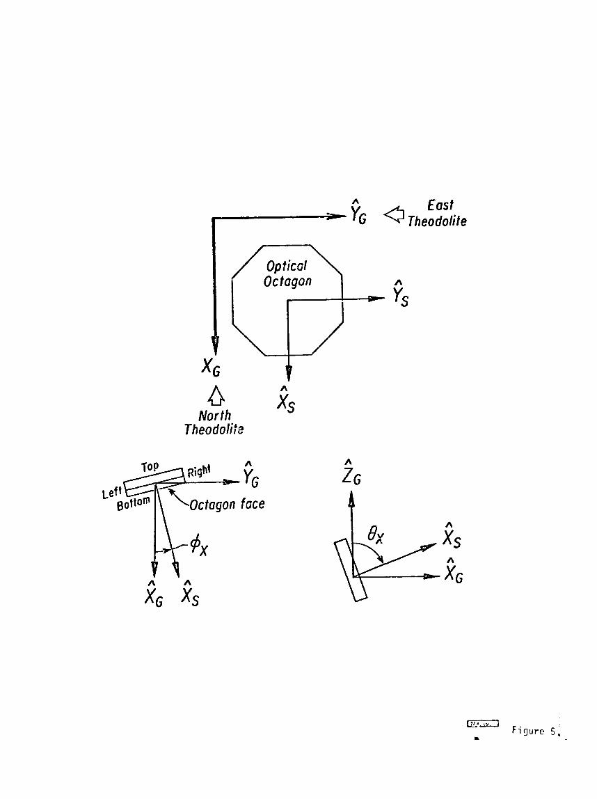
n East Y~ a ~heodoli fe

Theodolite

Figure 5, L

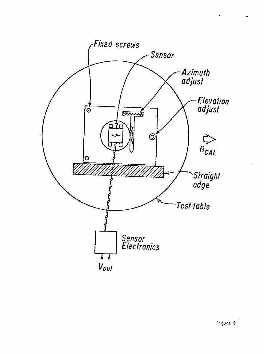
Figure 6

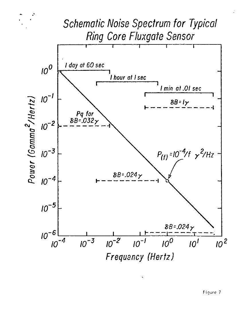
Schematic Noise Spectrum for Typical Ring Core Fluxgate Sensor

Frequency (Hertz)

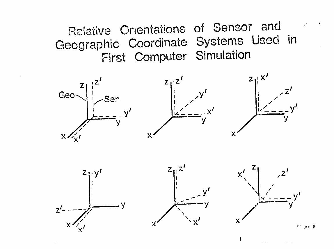
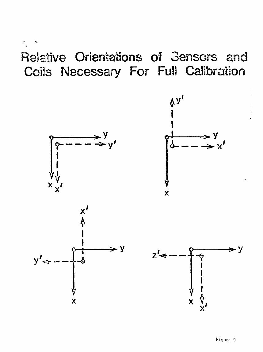
-a

~&lztive Orient ations of Sensors and Coils Necessary For Full Calibration

Figure 9

L i s t of Tables -

I. Transfgrmation na t r i c i t s used i n simlatod ca l i b ra t i on o f a s ing le

sensor wit!) a s ing le coil,

T T 2. Direction cosines of sensors (2 ) and c o i l s (rj ) zssuced i n

simulat ion o f f u l l ca l ib ra t ion .

3, Transformation i. .t - i c i e r f o r stv+n different r e l a t i v e o r ien ta t ioas

o f senscrs and c o i l s i n ful J car i b r d t i m -

4- Horra! ized rzasti;s-an:s for sev2;r 3 i f fe ren t o r i e n t a t i ~ n s of sensors

znd c o i l s - Ileading scross rad CWB i h t caasuremrnts corresp3nd EO

outputs o f sensors 1, 2, 3 for a f i e l d f i r s t i n coil 1, then c o i l 2

and f i n a l l y c o i l 3- They then repeae for t h e next r e l a t i v e

or ien:a t ions,

5 . Coefficients in the set of 9 equations produced by a f i xed o r i e n t a -

t i on of scnsors aqd co i ls , R%-J I and f o l . J refer to the trjo

matricies shown a t t h e botton-

6. Modif icat ions to be subtracted fro= the coefficients o f Table 5

caused by the use o f const ra in ts- The notat ion A318 r e f e r s t o the

9th ra: and l a t h colunn o f Table 5, and so on.

**

*

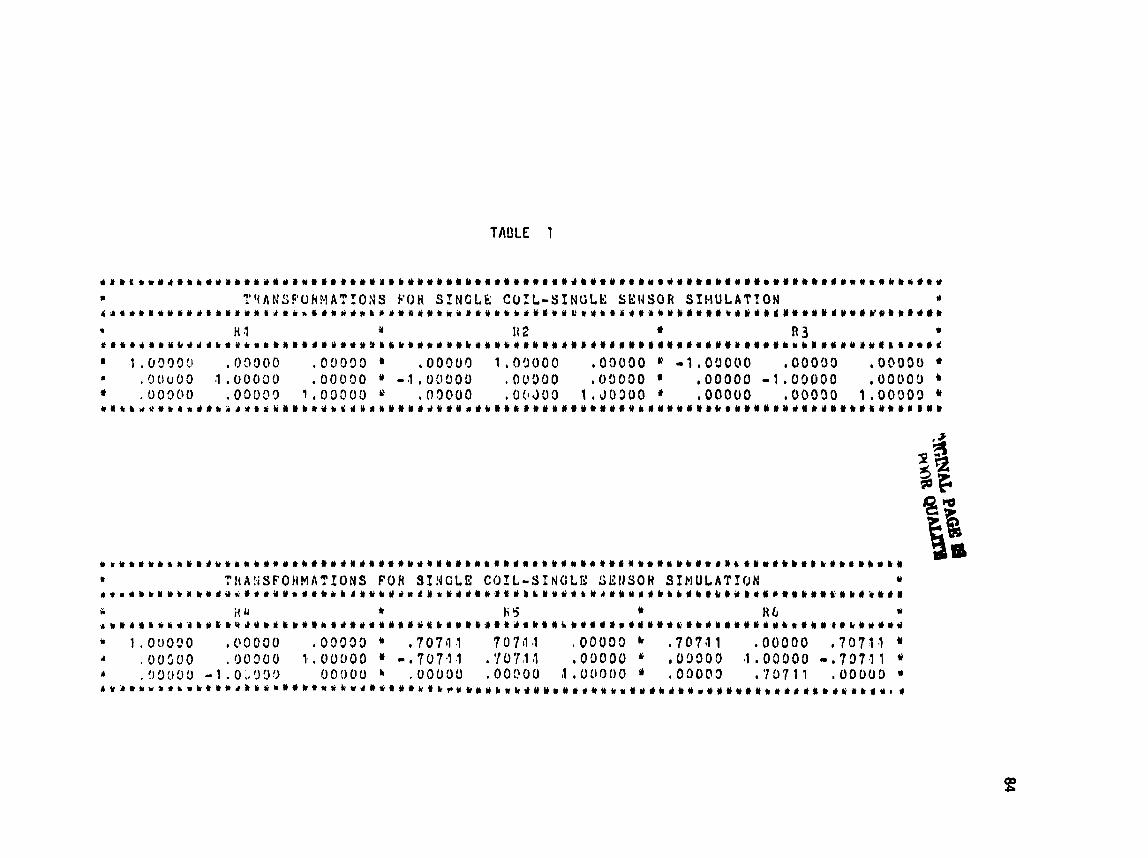
C

* * 1 -

a

* t

m

* a

Z

t

* 8

m

m

*

I

a

a

* I

* t

*

* Z

U

0..

* **

r t- r

*

4%

r lt

r 3-

r l*

an

*

r

v)*

1

a

t g1

0s

s -n

.r r z*

r

W7

r

;n

n

* - r ailr

2%

r 3

-

* 1 ,t

'L

r n

*

- I*

A

*

r

*4 *

3r

r u*

* r .it t

A

*

r U

*

* zt

*I -8

*

ma

*

0

* Z*

a ,?a

t T

*

I

* *

m*

*

zm

o

r

* C

(1

1

* e4 -*

* 4

*

* z

*

;L

v

13

4

* ,La

a

L9 *

* Z

*

* <*

*

z*

r i* r

1

* 1.

w

1

* -8

r

1

n

a

* n

t*

1

a

8

* I,

1

a a

m

.I 1

*a

*

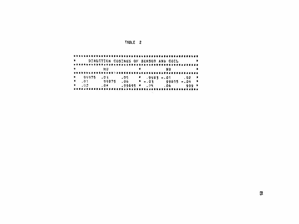
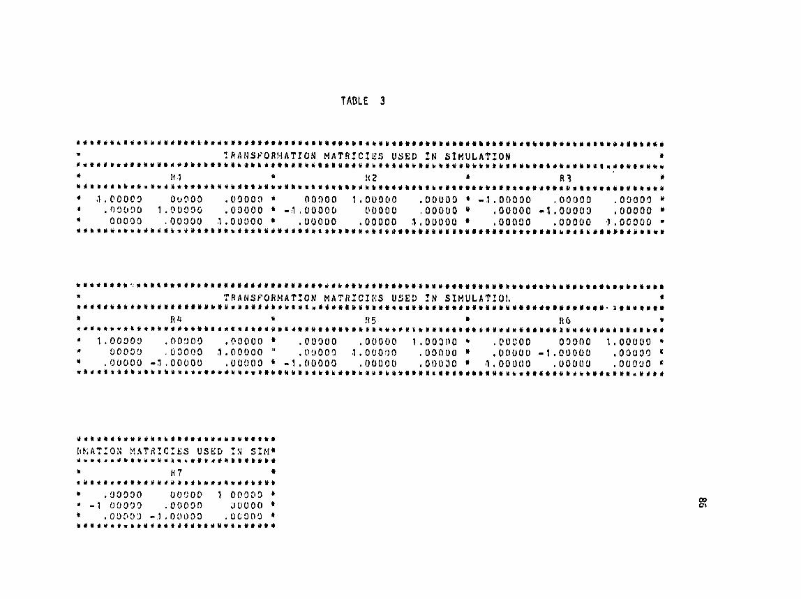
-1

.1

I

*

1

* t

I

* * * I

r

x

*.

t

* *

* *

1

* 1 *

t

I

1

a

t

* * t

* t

* *

a*

1

* A L

n

r 3

r

s

w+

a

r +a

14

-

= 2-

m 3-

r T

*

n*

r u

)z

* 1

* ZI

.) kt *

Ib

1

m

fa*

a izi*

* L?

a

a 3

r

a

* r cn*

a ~

1

r H

*

t Ur

* P

i =

t GI

+*

r u=

-a E I

* *

22

0-

t Cl -8

* e*

* ua

r

E*

r 4-

* 0

1

* r%

=

1,

ma

*

2*

* u*

* P

:*

r

C* o

I

* n

a

1

a

1

a

* *

* r

a

* *

* rr

* *

I

a

v

L

* .

c

* a

a

.I

* a

I

= Z

Z

* r.

w*

I

**

**

n

r 'z

- L ,+

JI

r Vl*

* *

* :7

*

n

LIi li

* rt

* a*

a a*

n

Vl*

*

3r

a

C

t *n

* kl*

1

t4

.r r U

+

* p

4.n

a

'L:.

a f-s

* e.

m

1 z*

a

* %

7

+O

r

I .i

1

r

C- v

u

48

m

zw

*

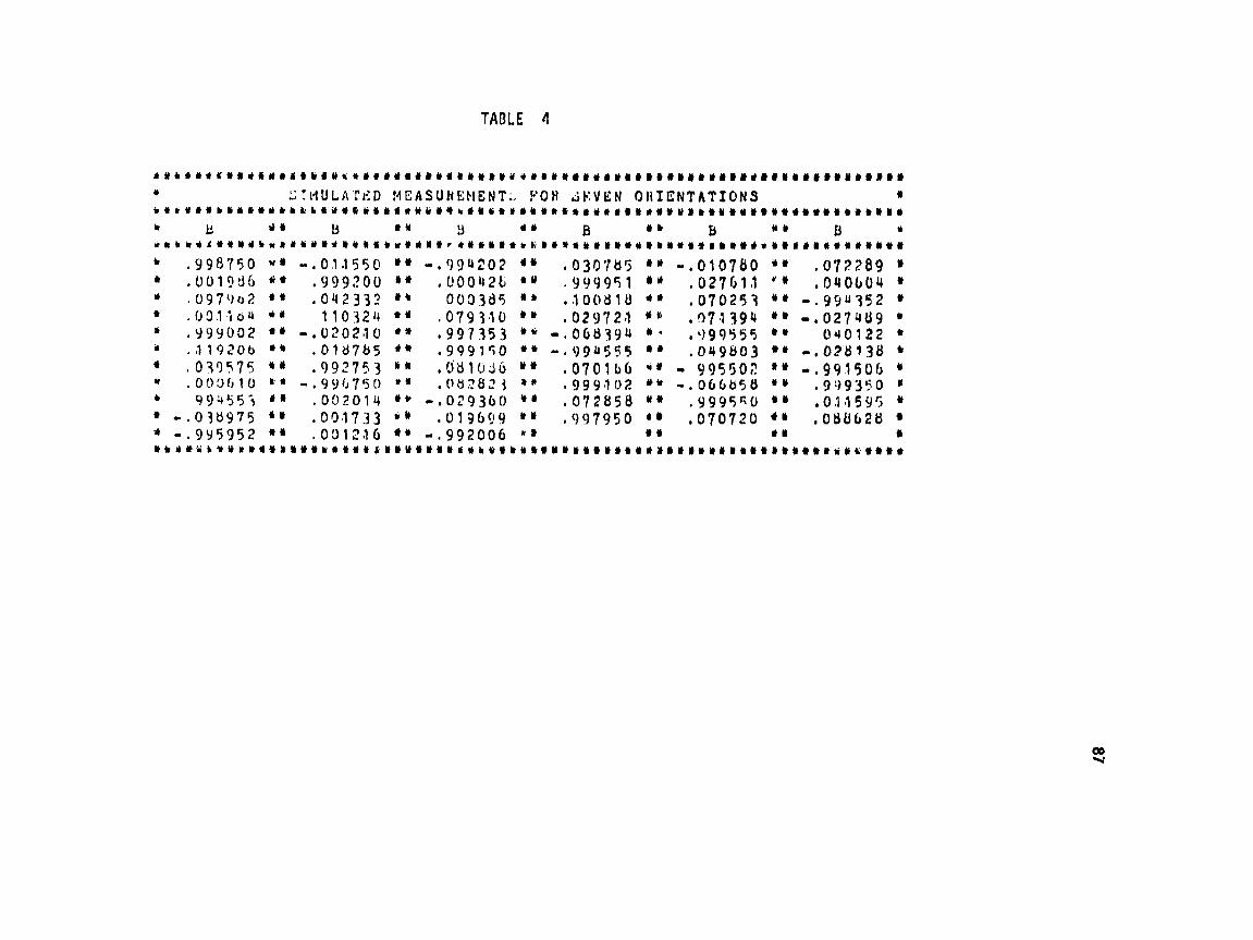
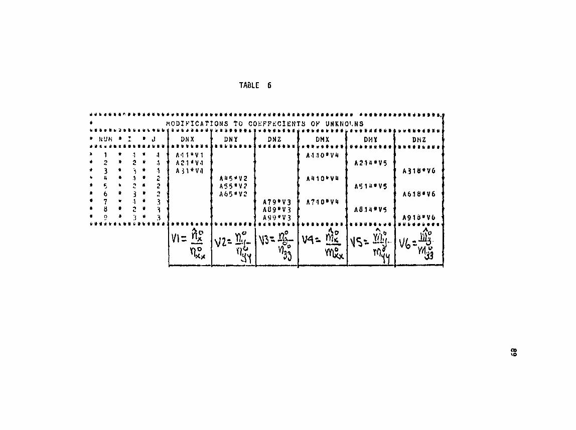
L i s t of Appendicies

A I. HAGSAT magne taae ter spec i f ica t ioils.

A2. S P E ~ E Z progratn "HAGSIW' which generates simulated sensor output

when excited by a cal ibration coil in a given orientation. fnputs-

are the direction cosines of the sensor and coi l i n the i r respective

coordinate systems -

A j . SPEAKEZ pragra "MGCAL 1'' which solves for the direction cosines

of sensor and co i l using i n i t i a l gwss and simulated measuresttnts,

Ah. SPEAKEZ program "tlEWSIWB which gtncra tes s imlated areasuremmts

for three sensar and three coi I sirailation-

AS. SPEAICEZ programs ''Ee3l tlPO ," "EQUATS ," and "SOLEQU-" Together these

programs use measurements of the transformation matrix and magnet-

ometer output with an i n i t i a l guess to solve for direction cosines

of three sensors and three coi ls .

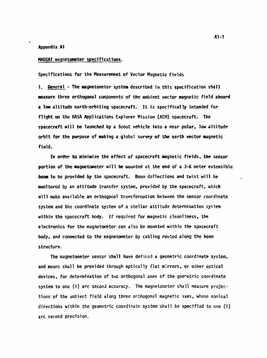
Appendix A1

MAGSAT magnetometer specifications.

Specifications for t h e Measurenrent of Vector Magnetic Fields

1. General - The m g n e t m t e r system described in th is specificatia? shall

seasure three orthogonal cmponents of the ambient vector magnetic field aboard

a low a1 ti tude earth-orbi ting spacecraft. I t i s speci fical ly intended for

f l ight MI the tiaSA Applications Explorer Mission (AEH) spacecraft. The

spacecraft will be launched by a Scout vehicle into a near polar, low altitude

orbit for t h e purpose of mking a global survey of the earth vector magnetic

field.

In order to mininrize the effect of spacecraft magnetic fields, the sensor

portion of the raagnetmeter will be munted a t the end of a 3-6 meter extensible

boom t o be pmvi&d by the spacecraft. Boon deflections and twist will be

monitored by an attitude transfer system, provided by the spacecraft, which

will make available an orthogonal trznsfomation between the sensor coordinate

system and the coordinate system of a s te l lar attitude determination system

w i t h i n the spacecraft body. If required fo r magnetic clean1 iness, the

electronics for the magnetmeter can also bc munted wf t h i n the spacecraft

body, and connected to the magnetometer by cabling routed along the born

structure.

The magnetometer sensor shall have defined a ge~metric coordinate system,

and means shall be provided through optically f l a t mirrors, or other optical

devices, for detemination of two orthogonal axes of the geopetr ic coordinate

system to one (1) arc second accuracy. The magnetometer shall measure projec-

tions of the ambient field along three orthogonal magnetic 3xes, whose nrwninal

directions within the gemetric coordinate system shall be specified to one (1)

arc second precision.

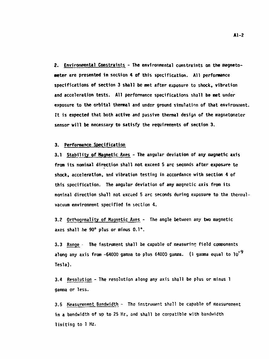
2. Envirortstental Constraints - The environmental cimstraints oft the Elagneto-

m t e r are presented i n set%ion 4 of t h i s specification, Bt 1 performance

specificartions of section 3 sha l l be met after exposure t o shock, v ib ra t ion

and acceleration tests. A1 1 performance speci f icat ions shall be met under

exposure to the orb i ta l thennal and under ground simulation o f t h a t environment.

I t i s expected tha t both act ive and passive thennal design o f the magnctmeter

sensor w i 11 be necessary t o sa t i s f y the requi remntr o f section 3,

3.1 - S t a b i l i t y of Magnetic Axes - The angular deviation of any magnetic axis

froln i t s nominal d i rect ion sha l l not exceed 5 arc seconds a f t e r exposare t o

shock, acceleration, and vibrat ion test ing i n accordance wi th section 4 o f

t h i s specification. The angular deviation o f any magnetic axis from i t s

nm ina l d i rect ion shal l not excxd 5 arc seconds during exposure t o the thernal-

vacuum environment specified i n 5ection 4.

3.2 Ortbogcmal i t y o f Magnetic Axes - The angle between any two magnetic

axes shal l he 90° plus o r minus 0. lo.

3.3 Range - The instrument shal l be capable o f measurinq f i e l d components

along any axis from -64000 gama t o plus 64000 gamna. (1 g a m equal t o l f 9

Tesla).

3.4 Resolution - - The reso l i~ t ion along any axis shal l be plus o r minus 1

gamna o r less.

3.5 Pleasurement Bandwidth- - The ins t ru isn t shol l be capable of mezsurenent

i n a bandwidth of up t o 25 Hz, and shall be conpatible with bandwidth

l i m i t i n g t o 1 Hz.

3.6 - Noise -- - Fluctuation noise associated w i t h any axis shall be less than

0.1 gamna xercr-to-peak when measured for 10 secor~ds i n a 25 Hz bandwidth.

3.7 Zero-Offset - The zero offset change associated w i t h any axis shall

be less than plus or minus 0.4 gaanra over the expected range of sensor and

electronics temperature. Long term s tabi l i ty of the zero offset shall be

less than 0.4 g a m fyear.

3.8 Absolute Accuracy - The total i n s t w ~ n t a l error from a1 1 sources i n

the determination of the field cmponent along any senscr geometric axis shall

be less than 5 gaarna. Th i s erwr budget inc:udes t h e effects of magnetic

axis stability, zero offset, fluctuation noise, quantization noise, sensitivity

changes, and a l l other purely f n s t m n t a l sources o f error.

3.9 Power Consumption - The total power consu~ption for the magnetmeter,

including power for normal controi o f the sensor, shall be less than 6 watts.

3.10 Weight - Total weight o f t h e system shall be less than 5 kilograms,

inclusive of the boom cable interconnecting sensor and electronics.

3.11 Volume - The sensor structure shall be cotitained within a 30 m,

diameter sphere, while the electronics package shall be contained w i t h i n a

volume 20 cin x 15 cm x 15 cm.

4. Environmental Requirements

4.1.1 Sinusoidal Vibration:

Frequency Level Sweep Rate Ax is - Range (Hz) 10 t o Peak) (OctfMin)

All ( X , Y , Z ) 10-18 5.0 g* 18-36 0.3 i n (O.A.) 4, 36- 150 20. g

150-2500 5- g * Limited to 0.3 in doub?e amplitude { D . A . )

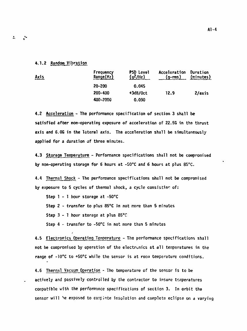
4.1.2 Random Vi_b~at ion

Axis - Frequency PSDLeve1 Acceleration Duration Range(Hz) ~ Q ~ / H Z 1 (9-rms) (minutes)

4.2 Acceleration - The performance specification of section 3 shall be

satisfied af ter non-operating exposure of acceleration of 22-56 i n the t h r u s t

axis and 6.06 i n the lateral axis. The acceleration shall be simultaneously

applied for a duration of three minutes.

4.3 Storage Temperature - Performance specifications shall not be compromised

by non-operating storage for 6 hours a t -50°C and 6 hours a t plus 8S°C.

4.4 Thermal Shock - The performance specifications shall not be compromised

by exposure to 5 cycles of thermal shock, a cycle consistinr of:

Step 1 - 1 hour storage a t -50°C

Step 2 - transfer to plus 85°C i n not more than 5 minutes

Step 3 - 1 hour storage a t plus 85°C

Step 4 - transfer to -50°C i n not more than 5 minutes

4.5 Electronics Operating Temperature - The performance speci fications shall

not be compromised by operation of the electrbnics a t a l l temperatures i n the

range of -70°C to +50°C while the sensor is a t room temperature conditions. - 4.6 Thennal Vacuum Operation - - Thc temperature of the sensor i s t o be

actively and passively controlled by the contractor to insure tctnperatures

compatible w i t h the performance specifications of section 3. In orbit the

sensor wi l l Fe exposed to COT ;ete insolation and cmplete eclipse on a varying

duty cycle basis. The extremes of the cycling are expected to be (a) a

continuous insolation for the indefinite period o f time and (b) sixty (60)

minutes of insolation to t h i r t y (30) minutes of eclipse.

ton/irmation of performance under there conditions will be perforxed by

the government during acceptance tests o f the magnetometer. The sensor w i l l

be operated a t pressure of 112 micron or less i n a ncn-magnetic thermal vacuum

system and rnagi~etic t es t faci l i ty i n chich the environment specified herein

shall be simulated by use of a liquid nitrogen shroud ar~d solar sixulatar.

During these tests, the electronics will be operated a t atmospheric pressure

and i n the temperature range -10°C t o +50°C.

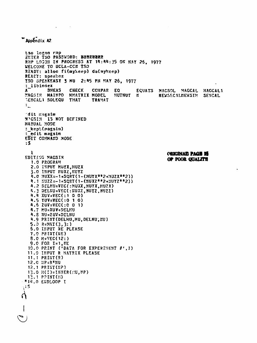
t s o Icson r s p ZXTER TSO PASPY3RD: BaBZB2LlZ -

RX? L%33 IH PRCCRESS AT 1 4 : 4 4 : 35 SAY 25, 1977 VELGO3E TC UCLA-CCC fS3 32RDY: alloc fi(aykeep1 da(ay9cep) REACY: speakcz TSO SPE!!.KfASY 3 #U 2:45 P 9 YAY 25, 1 9 7 7 : l i b i n d e x A- SHEAS CHECK COXPAR EQ ECQATS HXCSDL YACCAL HAGCALl X!iGSI:-! NAIHPO H t t t i T R I X XODEL YLTHUT t! #EYSECXLt!E'2SI2 SEWAL - E I O X L I SOLE CU TXXT T RAb4C.T -

' d i t asgsia Y'CSI:-i IS HOT DEFIHED WA??UXL :+ODE : - k e p : ( ? a g s i m ) : e d i t m a g s i m EBIT CO2ti4C3 XODE -(I - C

1 EDITISC ??AGSI#

1.0 P23GRkr-1 2.0 I!+PUT XUYX,NUf X 3.0 I?i P U T t jUXZ, CCYZ P .0 !-!UXX=-I +SQaT( l - ( N U Y X * * 2 + ~ - 1 ' J Z X * * 2 I ) 5 . 1 Z!jZZ=-?+SQ!?T( I - ( J ~ X Z t Z 2 + : ~ U Y Z i s 2 ) ) 9 . 2 GELHU=VEC(:3UXX,HUYX,F!UZX) &. 3 DELXU=VEC( :t!UXZ, #UYZ, t!fJZZ) 3 . 4 XUV=VEC(:I 0 0 ) 4.5 YUV=VEC(:O 1 0 ) 4.5 ZUV=VEC(:O 0 1) 4 -7 FU=XUV+9Et?:!J 4.8 XU=ZUV+3ELMU 4 . 9 PRI#T(DELNU,8U, DELMU, tZU) 5 . 2 3 = ; 4 a ~ ( 3 ,3 : ) 5 .0 IBPUT :iE PLEASE 7 . 0 ?RINT(i iE) 8 . C t ? = P f C ( 1 2 : ) 9.0 FO3 I=l,!!E

13.F FEINT ( 'DATA FOR EXPERI:?EMT # ' , I ) 1 1 . 9 f f ! P U T R ?!AT!3IX PLEASE 11.1 PRIliT(R) 12.0 :lP=B8!!U 1 2 . 1 PRIliT(!!?! 13.0 ;.;(I)=I?!:iER(l!U,t!P) 1 2 . 1 P?INT(F:)

= 1 4 . O EGDLOOP I :Sf

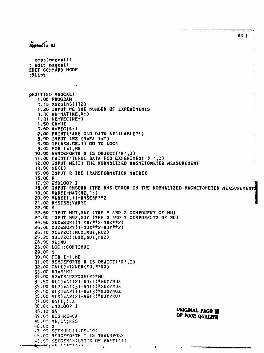
k e p ~ t n a g c a l l ) : e d i t m a g e a l l Es11 CC!+%A?!D HCOE :Sf ist

pEDZTISC 9AGCAL1 1-03 ?ROCRAY 1 - l o ~ ~ ~ c r n s ( t 3 2 ) 1.20 INPUT UE THE tiUHBER OF EXPERIHElTS 1-30 AA=HAT(#E,4:) 1.31 HE=VEC(HE: 1 1.50 tA=#E 1.63 A=VEC(4: 1 2.00 PRI i4T( 'A IE OLD DATA AVAILABLE?') 3-00 I X P U T b#S (O=Fd 1=T) 4-00 IF(AKS.CE.1) GO TO L O C I 9.03 FOR Zt1,lE

10.00 HEHCEFORTH R I S OBJECTf'R',I) 11.00 P R I J T ( ' 1 N F U I DATA FOR EXPERIXEXT f ' , I ) 12-00 IRPUT HE(I THS 3ORHALIZ ED #AG!#EIO*ETER WEASUREHENT 13.09 ? t E ( I ) 15.00 I N P U T R THE TELKSFOR?IATIOH HATRIX 16.00 R 17.00 E a m o o P I 18.09 fRPUT RYSERR (THE RHS ERROR 1% THE ROBYALIZED HACMETOHETER HEASU3E3EHT 19.03 VARYI=HAT(HE,l:) 20.09 VkRYI(, l)=R?fSERR**2 21.00 3XSERZ;VARYI 22.80 S 22.50 I t f P U T NUY ,PIG2 (TEE Y AH!, Z COHPC.IEFIT OF HU) 24.00 IWPUT MUX,;iUY (THE X AHD Y COYPOBEKTS OF NU) 24-50 XUX=SSRT( 1 -?IUY~'2-:4UZ~*2) 25.00 #UZ=SQRT ( I -HUX**2-HUY**2) 25-10 YLi=VEC(:#UX,#UY ,#UZ) 25.23 JU=VEC(:#UX,WUY,#UZ) 26.90 :4U;HU 25, '30 LOC 1 : COI:TIF!IiE 29.C3 $ 30.!?0 FCR I = l , N E 31,C3 HEHCEFORTH R IS O B J Z C T ( ' R t , I ) 32.00 C A ( 1 )=I ; l !JER(XU, R*t!U) 33-00 AI=S*NU 34 -09 R2=Ti#hP!SPOSf 34-59 A ( I )=A1(2 ) -A111)s~4UY/~4UX 35.00 A ( Z ) = A 1 ( 3 ) - A l ( l )s:4UZ/:*!UX 35-50 A(3)=Az(l)-A2(3)*HuX/NUZ 35.00 A(4)=A2(2)-AZ(?)*#UY/b!U?: 37.09 AA(I,)=A 38 -00 ZNDLOOP I 38.15 Ah 39.C? RES=EF-CA 45.99 YE;Ch;RES 46.~9 S 47."; SZTt lULL(1 .OE-10) 43 .W 3FXCZFORiTH T IS TR4t<SP9SE 43 . $ 3 SSZSZYhE4LYS:S OF AS~T(h.4)

ET-~-a~ a s * - - 8 - t n * 1 ! 1 I

3Z,WJ l U t Y 53.03 AUEYT=!tUEW A3-2

* S Y l O O UPrU 55-09 IEPUT LOWLIP? (LOULf 8 IS THE LOXEST ACCEPTBRLE EICE!IVlLUE 55.CQ LWdLIX 57 -03 ~HEWE(A~EV.LT.(LOYL~~~ AUEVf=O S S - ~ ru=t.ocs(Auen) 53.03 IF(IU(l).EQ.I) GO TO LOCAU 60-20 ItLOCS(~WT,AUEVT3 61.00 UP=U(,fU) 52.CO UO=U(,I) 53-00 LOCAU:CmTISU€ 64-39 $EICEHA3ALTSIS OF T(AA)sAA 65-00 AV=T(AAISAA 66-03 AVEV=EIGEHVALS(AV,V) 61.00 AVEV 68-09 AYEVT=IVZY 69-0t? VP=V 70.03 MHERE(AVEV,LT.LWdtrH) AVEYT=O 71-00 IV=LOCS(AYEYI) 72,CO IF(IV(lf,EQ,I) CO TO LOCAY 73-00 I=LOCSt-#OT,AWE\rr) 74-09 VP=Y(,IV) 75-03 vo=v(,r) 76-00 LOCAV:CO!iTItiUE 77.09 $SEE IF UP b#D YP GIVE A POS DEF DILC HAT 73-00 L=TCl!P)*kR.+VP 79-00 9E=DIfkGELS(L) m a o YHERE~DE-CT.O) DE=O 81-00 IFX=LOCS(DE) 82-00 $CHW?!GS SIGg OF COLWGS OF UP CCZRZSPCINDING TO BEGATIVZ EIGECYALUES 83-00 mo=noms(rFx) 84,C3 IF(IFXit)-EQ,@) G 3 TO 3ELW 85-00 FOR I=l,#DO 86.00 GP(,lFX(I))=-U?(,fFX(I)) 87-03 ENDLOOP I 83.00 SELW : COiJTI?:UE 83-09 L=T(UP)*AA*VP 9 0 . ~ 0 srncELs(t) 91 .OO f#VAA=VP*(I/L)"T(UP) 92-00 X=IHVAA"RES 33. GO N!?=?iORO!4S(IHVAb) 94 -00 YC=WOCOLS(INVAA) 93-10 92=HXT(NR,HC: 95-03 FOR I=l,lR 93.CO FOR J=l,MC 97.C3 H2(I,J)=IHVAA(I,J)*s2 93, C!0 E?:DLOOP J 99.00 E!IDLO3P 1 103. OD '#ARXK=H2"VA!lYI 101.00 SQRT(VARXK1 101.13 IF(fU(l)-EQ.l) GO TO HERE 102.03 VAR=(T(UO)*RES)'+Z 103.03 LRESSQ=RESQ*2 134.39 VAR;LRESSQ;VAR/LRESSQ 104.10 !-IERE:CONTIMUE 195.03 X 1O5.M t IUY=X(I)+NUY 135.50 :!UZ=X(2)+YUZ 137.03 ! X l X = X ( ? ) + Y U X 107. Sf1 fIUY = X (4 )+XLIY 122. CO :IUX=3C3T( 1 -? !UYw2-P?L'Zi*2) 193.50 :4UZ = S C ~ T (1 - F U X S V - ? l U Y ' x 2 ) 9 c.3 ~ ~ I I = Y E c ~ : ; . : ~ ~ ~ . : ~ u Y , ; ~ ~ , --,

-- 1 7 ---- ' I I

- -

. +-

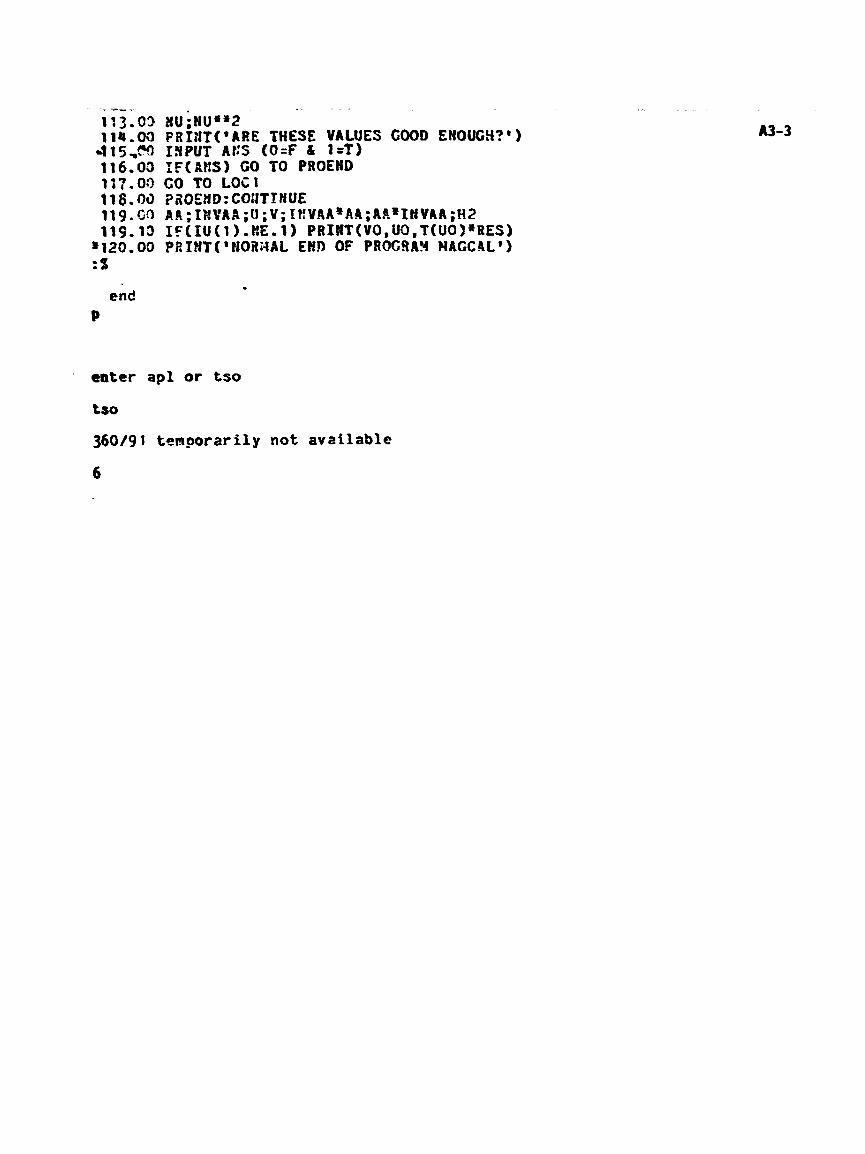
113.03 ~ u ; H u ~ ~ ~ 114.03 FRfffT( 'ARE THESE VALUES C06b EHOUGH?*) -~IS,CO InpuT A~:S {O=F & I=T) 116.03 IF[ACS) GO 13 PROEHD ttf.UQ co TO Lot1 116.03 3fOEHD:COITIHUE 119.00 AA; I#VAA;U;V; I~VAA*AA;AAi1HVAA;Hf 119.t3 IFfIU(l)-#E.I) PRIST(WO,UO,T(UO)"RES) 5120.00 PE IHT( 'MORi4AL END OF PROGRAY WACCLL' ) :s

end P

cnter apl or tso

tso

360/91 t cn~orar i ly not avzi lable

6

end Ed t4UXt HODE : e d i t ntwsim 4 IS EOT DEFINED g.: :!u A L n m : - kop:{newsfn) : e d i t neusim E F r r COHHAHD XUDE : s

1 EDZTXJG 3FdSIH

1 . 0 PSOGRAn 2.0 INPUT HUT A HAT WITH RQJS BEIMG UnfT VEC OF SEM I3 SEB C W R 3.0 ItiPUT HUT A ?tAT WITH ROYS BEING ti?iIT VEC OF COIL II CEO COOR 4.0 HENCEFORTH T IS TRRMSP 5.0 i + U = T ( # W ) ; H U = T ( n U T ) 6.0 H U ; I U 7 .0 SOBTIIH LIST DEFIWI?4C HUN OF SE?: ORIENT AND TRRCS HAT 8 . 0 KEPTLIST(TRAT) 9 .0 ROVS=9*SE

10.0 B=VEC(ROES: 1 1 1 . 0 $ 12.0 $LOOP TO CREATE HEASURENEHT EAT FOR CAI. ?4BT BC=X 1 3 . 0 L = 1 14.0 FOR K = l , t J E 14.1 P2I!:T ('EXPERIMEt4T B = ' K) 1 5 . 0 HEHCEFORTH R I S OBJECT('R*,K) 16.C 8%=3lUT*R*NU;BZ4 17-0 S IS. 0 S PUT COLUYtiS OF BX INTO COLU!4!1 VEC Of HEASU85HE!lTS 19.0 FOR J = 1 , 3 20.0 B(L)=BM(,J) 2 1 . 0 L=L+3 22.0 EJOLOOP J ; EHDLOOP X 23.0 SPaIMT AND SAVE THIS WECTO3

en*:! FAMURL MODE

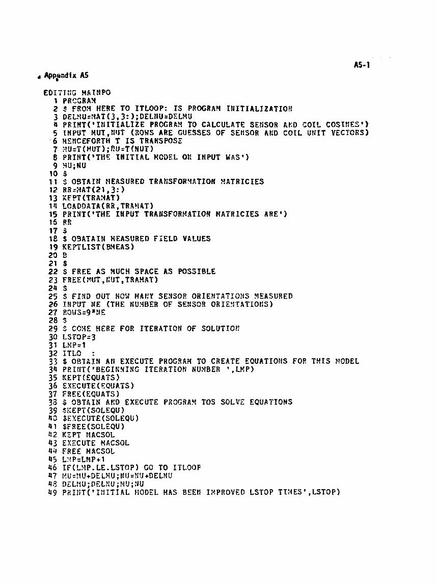
EUITTilC HAIHPO f PRCGRAPt 2 $ FRON HERE TO ITLOOP: IS PROCRAq Il4ITIALfZATfOW 3 D € L ~ U = : ~ A T ( ~ , 3: );QELkSU=DEtMU 4 PRIHT ( ' I N I T f A L I Z E PRCCRA?? TO CALCUtftTE SEfiSOI BED SO1 L COST!IES') 5 fNPUT PIUT,HIJT (EOWS ARE GUFSSES OF SEtlSOR At:D COIL UNIT VZCTCES) 6 HSHCEFORTH T IS TRAMSPOSf 7 :?U=T(MUT) ;f!U=T!NUT) 5 PRINI('THE INITIAL HCDZL 00 IHPUT MAS') 9 3U;KU

to S 11 $ OBTAIN MEASURED TR&HSFORHATfOE #ATRICIES 12 R3=:4AT(21,3: ) 13 EF PT (TRAHAT I 14 LCIDDATA(RR,TRh?-!kT) 15 PRI3T('PHE IHPUT TR&NS€ORHdTIO% NATRICIES ARE') 15 it: 17 s 18 $ O 9 A T A I H HEASURED f IELD VALUES 19 KE?TLIST(&YEAS) 29 Q, 21 S 22 $ FREE AS NOCY SPACE AS POSSIBLE 23 FREE(HUT, t:UI, TRkHAT) 24 S 25 $ F f 3 D OUT HOW HAt!Y SENSOR OBIEHIATIO3S YEASURED 26 INPUT HE (THE MUYBER OF SECSOR 03fE!!TATIOt!S) 27 R3W3=9*3f 28 S 29 S CC3E HERE FOR ITERATIOH OF SOLUTIC?! 30 LSTOP=3 31 Ltl;P=t 32 ITLC! : 33 $ ORTkIN A N EXECUTE PROGRAH TO CREATE EOUATIOHS FOR THIS NODEL 34 PLItiT( 'BEGIRYISG ITERATEO!I WUXBER ' , L X P ) 35 SEPT(EQUAIS) 36 EXECUTE (FQUAIS) 37 fREE(EQUATS) 33 5 OBTkIN A E D EXECUTE PROGRA?I TOS SOLVE EQUATIOMS 30 $XEP'i(SOLEQU) 43 3EXECUTE(SOtEQU) 4 1 $FSEE(SCLEQU) 92 KEPT MACSOL 43 EXECUTE MACSOL 43 FREE HACSOL 45 L:-lP=LMP+1 46 ZF(L?!P.LE.LSTOP) CO TO ITLOOF 47 !!U=:Il!+DELMU; t!lJ=?fU+DEL?#U 49 DEL:tU;DEL:;'U ;MrJ;:IU 49 PRItjT( '1 :]IT1 AL MODEL HAS BEEtf 1 XPROVED LSTOP T'I:4ESf ,LSTOP)

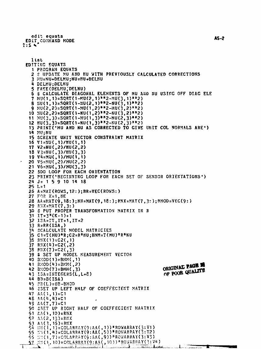
e d i : equats ED1 T, CQ:-IRAED NODE

5 . c i . r 4

1 ist EDITI?lC E Q U A T S

1 PZC!G!td!4 E O U A T S 2 3 UPDATE XU AUD HU YITH PREVIOUSLY C A L C U L A T E D CORRECTIONS 3 Z!J=SU+DELHU ;? iU=?!U+DEL8U 4 DELF?U;DELF!U 5 F i z f E ( E I E L ? ! U ; D E L I U ) 6 $ CALCULATE DXACOHAL ELENENTS OF NU XiiB t iU USTCC O F F DXkC ELE 7 ~~(l,1)=sQsr(l-#u~2,l)**2-~4u(3,1)1+2) B ? ; U ( l , l ) = S Q R T ( l - X U ( 2 , 1 1 4 * 2 - N U ( 3 , 1)**2) 9 EU(~,~)=SQRT(~-~U(~,~)'"~-I~U(~,Z)~Z)

10 ? i ~ ( 2 , 2 ) = S Q R T ( l - # U ( t , 2 ) *"2-NU (3,2)3*2) 11 3!!(3,3)=SQ~T(1-~3(1,3)*'2-?iU(2,3)"2f 12 H u ( ~ , ~ ) = S Q R T ( ~ - ! ~ U ( I ,3)*'2-!fU(2,3)si2) 13 P R I K T ( ' H U AKD %U AS C O R R E C T E D TO G I V E UCIT COL HORYALS A R E ' ) 14 :-lk!;HU 15 $CREATE UNIT VECTOR C O N S T R A I N T MATRIX 16 i ' l = ? i t i ( , l ) / ! W ( l , l ~ 17 V Z = N U ( , Z ) / H U ( 2 , 2 ) 18 v?=nu(,3)/nu(3,3) 19 v G = x a ( , l ) / n u ( i , l ) 20 V 5 = N U ( , 2 ) / H U ( 2 , 2 ) 21 vs=:4ut , 3 ) / H U ( 3 , 3 ) 22 $DO LOOP FOR EACH O R I E H T A T I O N 23 PRIMT('BEG1WNIt~C LOOP F O B EACH S E T O f SSRSQa ORIEETATIGMS') 24 J = 1 5 9 10 14 18 25 L = l 25 k=:-?Af (ROXS, 12: );BR=VEC(R3YS: ) 27 Fez X = 1 , tlE 28 A A 4 = X A T ( 9 , 1 8 : ) ; ~ 3 = ~ A T ( 9 , 1 k ) ; R N X = X A T ( 7 , 3 : );B:=lOD=VEC(g: ) 29 FiYX=2AT(?, 3: 30 $ PUT PRCPER TRANSFORHATIO!i H A T R S X 18 R 31 I T = ? " ( ! C - l ) + I 32 ISA=IT , I T + I , IT+2 33 R = R R ( I S A , ) 34 SCILCUL4TE M O D E L MATRICIES 35 C1=T(XU)+R;C2=R*flU;BXH=T(MU)*RsUU 25 R ? I X ( I ) = C 2 ( , 1 ) $7 R Y X ( 4 ) = C 2 ( , 2 ) 38 P ? : X ( 7 ) = C 2 ( , 3) 39 $ 3ET UP M O D E L K E A S U R E Y E E I T V E C T O f i 40 3 X 3 D { l ) = B W : 4 ( , 1 ) 41 8:.!00(4)=8P!b?( ,2) 42 3XCD(7)=BMH( ,3 ) 43 Z S A = I : i T E C E R S ( L , L + 8 ) 44 03=3(ISk) 45 ?2(L)=OE-E:33D 46 $3 fT UP L E F T H 4 L F OF COEFFECIEFT HATRIX 47 A.4( 1.1 ) = C 1 4 8 ? A ( S t 4 ) = C 1 - 49 A 4 ( 7 , 7 ) = C 1 50 $557 UP RIGHT HALF OF C O E F F E C I E N T M A A T R I X 51 L3.C 1 , 13 ) = R ? l X 52 A5.(2, l ? ) = R t l X

- - - - -- 7-

5 t J t A = E L f > l C O L S ~ A A , d l A5-3

bc'iAfL,lI=AA i 63 L=L+9 60 6;iDLOOP # 65 Re i 65 FRZE(V1 ,V2,V3,V4,V5,V&J,R,AAtEP!,ZT,IS4,R,Cl,C2,5~4~~I,RHX,0~S9,BBI !

'67 PBIIIT( 'PROGRArl EPUATS HllS CORPLETED CALCULATIOC OF EQUATIORS FOR THIS . C . L

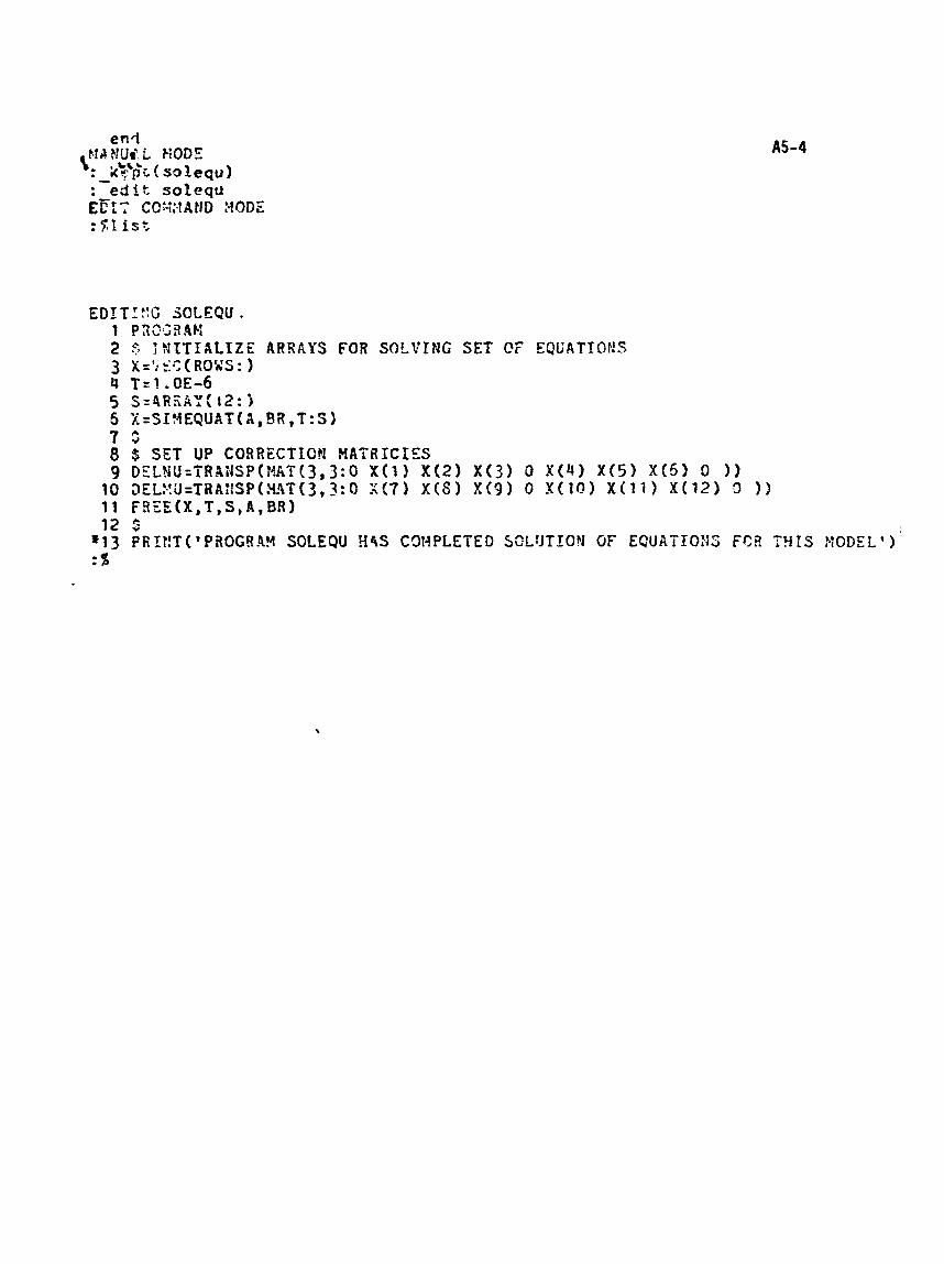
en4 81d ?f!Lfd. i NOD5 : - kyi;c< ro lequ) : e d i t solequ EFT^ CC;*?:-t AMD NODE :Flis';

EDIII!!C 3OLEQU . 1 P32ZRA1.I 2 $ I NITIXLIZZ ARRAYS FOR SOLVING SET OF EQtiATIOb!S 3 X=':r:C(R3'2r'S:) 4 T=?.OE-6 5 S=4RSAY( 12: ) 6 X=SI!iEQUAT(X,BR ,T:Sl 7 $ 8 $ SET UP CORRECTICH MATRICIES

DELnU=iffXi4SP(l!AT(3,3:0 X(1) X(21 X ( 3 ) O X ( 4 ) X ( 5 ) X ( 5 ) !I 1) 10 3EL:!3=TRA:!SP(X4T(3,j:O X ( 7 ) X ( 8 ) X ( 9 ) 0 X ( 1 0 ) X ( 1 l ) X ( 1 2 ) 3 ) ) 11 F!iEE(X,T,S,A,BR) 12 $

*I3 PRf CT('PFtOGSAY SOCEQU HtS COt4PLETED SOL!JTIO?i OF ECUATIO3S FC? 191s MODEL' ) : 5