Embed Size (px)
Citation preview

Diss. ETH Nr. 10277
A Programming Language for Vector Computers
A dissertation submitted to theSWISS FEDERAL INSTITUTE OF TECHNOLOGY ZURICH
(ETH Zürich)
for the degree ofDoctor of Technical Sciences
presented byRobert Griesemer, Dipl. Informatik_Ing. ETH
born June 9, 1964citizen of Güttingen, Thurgau
accepted on the recommendation ofProf. Dr. H. Mössenböck, examinerProf. Dr. N. Wirth, co_examiner
1993

Copyright (c) Robert Griesemer, 1993

5
Acknowledgements
This work would not have been possible without the help and encouragementof many people. I am most indebted to Prof. H. Mössenböck for his continuoussupport and his insistence on clarity and simplicity. If this thesis is moreunderstandable now, this is due to his constructive criticism. I also would liketo thank Prof. N. Wirth for a liberal supervision of this project and for posingthe right questions at the right time. His comments lead to a much better andclearer understanding of what programming is all about.
It is a pleasure to mention my colleagues of the Institute for ComputerSystems; they cared for an agreeable and inspiring environment and many ofthem contributed to this work. Clemens Szyperski and Josef Templ constructedthe tools for preparing this document, namely the excellent Write textprocessing system (Clemens) as well as the unique graphics editor Kepler(Josef). Marc Brandis was a well_versed discussion partner in all kinds ofcompiler related topics. The Oberon_2 compiler used for the implementationwas developed by Régis Crelier and would pass industrial strength tests.Matthias Hausner readily adapted the Write editor to even higher requirements.Ralph Sommerer implemented some tools to create amazing Mandelbrotpictures from incredibly long Cray output. Wolfgang Weck and PhillippHeuberger helped with their experience in theoretical issues.
Bernd Mösli and Urs von Matt gave valuable hints on the requirements ofnumerical applications. Marc Brandis, Régis Crelier, Kathrin Glavitsch, JosefTempl, and my brother Marcel carefully proofread parts of this thesis. AlbertWeiss and Immo Noack cared for a frictionless operation of the hardware. Forvarious fruitful discussions and suggestions I would also like to thank Dr. S. E.Knudson, B. Loepfe, Prof. Dr. B. Sanders, and Dr. A. Schei. Several studentscontributed also to this work, namely Jürg Bolliger, Hugo Hack, Patrick Spiess,and Roger Waldner.
Last but not least, my warmest thanks go to my life companion Sabine forher patience and love through all the time.

6
Contents
Abstract 8Kurzfassung 9
1 Introduction 111.1 A Hypothetical Vector Computer 121.2 Vectorization: An Example 161.3 Vectorization of Fortran DO Loops 191.4 Vectorization of Fortran 90 Array Expressions 231.5 Array Parameters in Fortran 24
2 A Language Proposal 272.1 The ALL Statement 272.2 Array Constructors 322.3 Differences between Oberon and Oberon_V 35
2.3.1 Basic Types 352.3.2 Pointer Types 372.3.3 Procedure Types 382.3.4 Structure Assignment 392.3.5 Character Sequences: The Exception 402.3.6 LOOP Statements Considered Harmful 412.3.7 Side_Effect Free Functions 42
3 Implementation 433.1 Linear Functions 433.2 Affine Functions 453.3 Representation of Expressions by Expression Trees 463.4 Compilation of Range Declarations 483.5 Linear Range Expressions 513.6 Reorganization Properties of ALL Statements 523.7 Translation of ALL Statements into Vector Instructions 55
3.7.1 1_dimensional ALL Statements 563.7.2 n_dimensional ALL Statements 593.7.3 Interesting Cases 66
3.8 Compilation of Array Constructors 683.8.1 Array Variable Constructors 683.8.2 Array Value Constructors 75
3.9 Index Checks 78
7
4 Related Work 83
5 An Oberon_V Compiler 915.1 Modularization 925.2 Intermediate Program Representation 94
5.2.1 Representation of Objects 955.2.2 Representation of Types 1025.2.3 Representation of Statements 1065.2.4 Representation of Entire Programs 1105.2.5 Import and Export 111
5.3 Code Generation 1125.3.1 OVC: High Level Code Generation 1125.3.2 OVE: Expressions 1155.3.3 OVV: The Virtual Machine Code 120
5.4 Hardware Support 129
6 Measurements 1316.1 BLA Subprograms 1316.2 Linpack Subroutines 1346.3 Compiler Data 137
7 Summary and Conclusions 1397.1 What has been achieved 1397.2 What could be improved 1417.3 Conclusions 142
Bibliography 145Appendix A: The Programming Language Oberon_V 153Appendix B: Program Examples 189

8
Abstract
This thesis introduces and elaborates on specific language constructs that allowa simple programming of vector computers and help to gain a betterunderstanding for these programs. Thereby the emphasis lies on the support ofexplicitly vectorizable statements as well as on a concept for parameter passingadapted to the needs of numerical applications.
Vector computers provide powerful instructions for the processing of wholevectors. The speed of programs is often increasing by orders of magnitude ifthese programs allow the use of such instructions, i.e. if they are vectorizable. Inorder to make a program run faster, a compiler usually tries to vectorize itsinnermost loops. Unfortunately, the dependence analysis required therefore isquite complicated and often cannot be performed completely. The thesistherefore proposes a simple language construct allowing the explicitspecification of independence and thus the parallel execution of statements.Hence, this language construct is much easier to vectorize than loops. Itimproves the readability and security of programs without reducing the qualityof the generated code.
The main application area of vector computers are numerical applications oflinear algebra. A problem arising with those programs is that parts of matricessuch as rows, columns or diagonals must be passed as arguments to asubroutine. Yet, most programming languages do not support such a flexibleway of parameter passing. Array constructors offer a simple and safe way tosolve this problem.
The second part of the thesis focuses on the description of an experimentalprogramming language called Oberon_V and of an appropriate cross_compilerfor the Cray Y_MP. Oberon_V includes a subset of the language Oberon, whichhas been extended by the language constructs mentioned above. Compared totraditional compilers for vector computers, the Oberon_V compiler excels by itscompactness and efficiency. Detail problems of implementation were solved ina new and more simple way: some of the achievements were a new way ofgenerating symbol files to support separate compilation, the optimization of thegenerated code by eliminating redundant computations (commonsubexpression elimination) and the reorganization of instructions to increasethe execution rate (instruction scheduling). The thesis finally investigates andjudges the code quality of Oberon_V programs in comparison withcorresponding Fortran programs.

9
Kurzfassung
In dieser Arbeit werden spezielle Sprachkonstrukte eingeführt, die das einfacheProgrammieren von Vektorrechnern erlauben und zu einem besseren Verständ_nis dieser Programme beitragen sollen. Im Vordergrund steht dabei die Unter_stützung von explizit vektorisierbaren Anweisungen sowie ein an die Bedürf_nisse numerischer Applikationen angepasstes Parameterübergabe_Konzept.
Vektorrechner stellen leistungsfähige Instruktionen für das Bearbeiten ganzerVektoren zur Verfügung. Programme werden oft um Grössenordnungen schnel_ler, wenn sie von solchen Instruktionen Gebrauch machen können; d.h. wennsie vektorisierbar sind. Zu diesem Zweck versucht ein Compiler gewöhnlich dieinnersten Schleifen eines Programms zu vektorisieren. Die dazu notwendigenAbhängigkeits_Analysen sind kompliziert und können häufig auch nur unvoll_ständig ausgeführt werden. Es wird ein einfaches Sprachkonstrukt vorge_schlagen, welches die Unabhängigkeit und somit die parallele Ausführbarkeitvon Anweisungen explizit auszudrücken erlaubt, und deshalb wesentlicheinfacher vektorisierbar ist als Schleifen. Es wird gezeigt, dass damit die Qualitätder Programme bezüglich Lesbarkeit und Sicherheit verbessert werden kannohne dabei die Qualität des erzeugten Codes zu vermindern.
Hauptanwendungsgebiet von Vektorrechnern sind numerische Applika_tionen aus dem Bereich der linearen Algebra. In solchen Programmen stellt sichoft das Problem, dass Teile von Matrizen, z.B. Zeilen, Spalten oder Diagonalenals Argumente einem Unterprogramm übergeben werden müssen. Die meistenProgrammiersprachen unterstützen eine solch flexible Art der Parameterüber_gabe nicht. Mit Hilfe von Array_Konstruktoren lässt sich dieses Problem einfachund vor allem sicher lösen.
In einem zweiten Teil der Arbeit wird eine experimentelle Programmier_sprache (Oberon_V) sowie ein dazugehörender Cross_Compiler für die CrayY_MP vorgestellt. Oberon_V umfasst eine Teilmenge der Sprache Oberon, welcheum die erwähnten Sprachkonstrukte erweitert worden ist. Der Oberon_VCompiler besticht durch seine Kompaktheit und Effizienz im Vergleich zu her_kömmlichen Übersetzern für Vektorrechner. In der Implementierung wurdendiverse Detailprobleme auf zum Teil neue und einfachere Art und Weiserealisiert. Dazu gehören eine neue Art der Erzeugung von Symbol_Files für dieUnterstützung getrennter Übersetzung, die Optimierung des erzeugten Codesdurch Entfernen redundanter Berechnungen (Common Subexpression Elimina_tion) sowie das Umordnen von Instruktionen zur Steigerung der Ausführungs_geschwindigkeit (Instruction Scheduling). Schliesslich werden Oberon_VProgramme sowie die erreichte Codequalität im Vergleich zu entsprechendenFortran_Programmen untersucht und kritisch beurteilt.


1 Introduction
"As soon as an Analytical Engine exists, it will necessarily
guide the future course of science. Whenever any result is
sought by its aid, the question will then arise − by what
course of calculation can these results be arrived at
by the machine in the shortest time?"
Charles Babbage − The Life of a Philosopher, 1864
With the development of vector computers and massively parallel machines,highly computing_intensive applications have become feasible withinreasonable time bounds. Since numerical programs constitute the major part ofall applications on these machines, the programming language Fortran is usedin most cases, despite its shortcomings.
While it does not seem clear yet which is the best way to program massivelyparallel machines, the programming of vector computers is comparatively wellunderstood. This thesis concentrates on vector computers only. Since Fortran77 [Brainerd et al. 1978] provides no special language support for thesemachines, an optimizing compiler typically tries to vectorize innermost DOloops; i.e. it tries to restructure the program in order to allow vector instructionsto be used instead of scalar instructions. It is highly desirable to have as manyvectorizable loops as possible since the execution speed of such loops may bemore than a decimal order of magnitude higher than the one of conventionallytranslated loops. Unfortunately, the necessary dependence analysis is quitecomplicated, and often it cannot be decided whether it is possible torestructure a loop without affecting its semantics, in which case it must beexecuted sequentially. Therefore, a Fortran programmer has to carefully avoidany constructs within innermost loops which may inhibit vectorization. In fact,he must know how the specific compiler in use does vectorize. It would ofcourse be better to use a suitable language construct instead. The features ofFortran 90 (see e.g. [Metcalf 1987]) reduce this problem a little bit. However, aswill be shown in Section 1.4, Fortran 90 array expressions require dependenceanalysis, too.
This thesis introduces a new language called Oberon_V, based on theprogramming language Oberon [Wirth 1988a]. The principal new features of

12 Introduction
Oberon_V are its ability to directly express potential parallelism in assignmentsand a construct to specify subarrays which may be passed as arguments toprocedures. The former allows for efficient translation into vector instructionswithout dependence analysis, whereas the latter is an essential prerequisite forthe programming of numerical applications (which was missing in Oberon'spredecessors Modula_2 [Wirth 1985a] and Pascal [Wirth 1971]). Theresponsibility for the correctness of parallel executable program parts isdelegated to the programmer. This decision is justified by practical examples ofrealistic programs.
The thesis is organized as follows: in the first two sections a hypotheticalvector computer will be introduced, allowing to illustrate the basic concepts ofsuch machines and serving as a basis for (vector) code examples. The problemsarising when trying to vectorize DO loops are illustrated in Section 1.3. A specialfeature of Fortran 90, so_called array expressions, is investigated in Section 1.4,whereas Section 1.5 shows the problems of passing (sub_)arrays to subroutinesand procedures. Chapter 2 describes the main concepts of Oberon_V; possibletranslation schemes are shown in Chapter 3. A survey of related programminglanguages may be found in Chapter 4. Chapter 5 describes the overall structureof a complete Oberon_V compiler called OV for the Cray Y_MP [Cray 1988].Measurements made on a small collection of typical programs compiled withOV are arranged and discussed in Chapter 6. The thesis ends with theconclusions in Chapter 7. The Oberon_V language report may be found inAppendix A. Several typical programs are contained in Appendix B.
1.1 A Hypothetical Vector Computer
The topics of this thesis are programming languages and vector computers.While it is assumed that the reader has a certain understanding of what aprogramming language is, the notion of a vector computer might not be asclear. For the purpose of abstraction, a hypothetical vector computer isintroduced that will be used instead of a real machine architecture that wouldhave to be explained in full detail and with all its deficiencies. As a simplejustification, it is stated that this machine reflects the basic programming model
of many modern (register_to_register) vector processors, including machinessuch as Cray_1 [Russel 1978], Cray Y_MP [Cray 1988] and Cray_2, or NEC SX_2and NEC SX_3 [NEC 1989]. In the following, the term vector computer alwaysrefers to this machine model, unless it is explicitly specified otherwise.
All vector computers share the concepts of vectors to which vector
instructions can be applied. A vector is a finite sequence of scalar values called

13Introduction
elements. It may be held either in a vector register or in memory. In the lattercase, a vector is determined by its starting address c0, a stride c1 and its length l.The starting address is the address of the first element in memory whereas thestride specifies the (possibly negative) constant address difference between twoconsecutive elements in memory. The length is the number of vector elements(Figure 1.1).
stride
increasing address...
starting address
v v v v0 1 2 l−1
Figure 1.1 Memory Mapping of Vectors
In analogy to the notion of a variable address, the term vector address is used forthe pair (c0, c1). Obviously, the set of addresses of all vector elementscorresponds to the range of an affine function f(x) = c0 + c1x with x restricted tothe set {0, 1, ... l−1} (see also Section 3.2).
Scalar
Functional
Functional
Vector
Units
Units
M
E
M
O
R
Y
0 1 2 3 ...
VL
VLmax
−1
...
S6
S5
S4
S3
S2
S1
S0
...
V6
V5
V4
V3
V2
V1
V0
Figure 1.2 Hypothetical Vector Computer

14 Introduction
The length of vectors held in main memory is virtually unlimited whereas vectorregisters may only hold vectors of a certain maximum length VLmax. Besides theregisters for scalar values, a vector processor provides a special register fileconsisting of vector registers. For simplicity, it is assumed that both the scalarand the vector register file provide an unbounded number of registers; theformer are denoted by S0, S1, etc., the latter by V0, V1, and so on (Figure 1.2).
The power of a vector computer lies in the vector instructions. A vectorinstruction is a machine instruction that performs an operation on an entirevector. It may be a vector load or store instruction to access (parts of) vectors inmemory or scalar operations applied element_wise to their operand vector(s). Aspecial vector length register VL is used to specify the number of elements to bemanipulated by a vector instruction.
On a real machine, scalar and vector instructions are executed by thecorresponding functional units. Since the execution of an instruction may takemore than a single clock cycle (this is especially true for vector instructions),functional units are segmented and the instructions are executed in a pipelined
fashion. Furthermore, if different functional units exist for different operations(e.g. an add and a multiply unit), different operations can be executedconcurrently. It is this parallelity on the instruction level combined with thepossibility to issue a sequence of operations by a single vector instruction thatleads to the significant speedup of vector computers. However, timing aspectsare not of relevance here. They will be discussed later. The hypotheticalmachine provides the following instruction classes:
Class Instruction
scalar operations Si := Sj op Skscalar comparisons Si := Sj rel Skscalar load Si := M[Sj + Sk]scalar store M[Sj + Sk] := Sivector operations Vi := Vj op Vkvector comparisons Si := Vj rel Vkget vector element Si := Vk[Sj]set vector element Vi[Sj] := Skvector load Vi := M[Vj, Sk]vector store M[Vj, Sk] := Viset VL VL := Sjget VL Si := VLvector merge Vi := Vj | Vk (Sl)jumps jump Sj (˜Sk)

15Introduction
With the exception of jumps, the instructions are to be read as assignments.The letters i, j, k and l stand for a register number and the operand position; opdenotes an arithmetic or logic operation and rel stands for one of the relations=, 9, <, #, > or 3. A Vj operand may be substituted by an Sj operand. Whereveran Sj operand is expected, an immediate value x (i.e. an integer constant) maybe used instead. An Sk or Vk operand may be substituted by the immediatevalue 0. In the examples, a zero operand will be simply omitted. A scalarcomparison "Si := Sj rel Sk" yields 1 or 0 depending on whether the relation istrue or false.
The vector instructions deserve a more precise explanation: every instructionis executed for as many vector elements as specified by the current value of thevector length register VL. A vector operation of the form "Vi := Vj op Vk" (or "Vi:= Sj op Vk", obtained by substitution of Vj by Sj) is to be understood as "Vi[e]:= Vj[e] op Vk[e]" (or "Vi[e] := Sj op Vk[e]" respectively) for all values of e in theset {0, 1, ... VL−1}. A vector load instruction of the form "Vi := M[Vj, Sk]" is tobe read as "Vi[e] := M[Vj[e] + Sk]"; hence the address of the element e iscomputed by the value of the element e of Vj plus the value of Sk. This issometimes called a vector gather operation. A similar interpretation of thecorresponding store operation leads to a vector scatter operation. By substitutingthe Vj operand with Sj, the conventional vector load/store instructions areobtained: e.g. "Vi := M[Sj, Sk]" is to be read as "Vi[e] := M[Sj*e + Sk]"; i.e. Skdenotes the starting address of the vector whereas Sj denotes its stride. Aconstant stride is expressed by simply using an immediate operand instead ofSj. Hence, the pair (Sk, Sj) represents the vector address.
Vector comparisons "Si := Vj rel Vk" are used to compare entire vectors. Thebit e of the destination register corresponds to the result of the comparison ofvector element Vj[e] with vector element Vk[e]. If the comparison yields true,the corresponding bit is set to 1, otherwise it is set to 0. This instruction isuseful for the implementation of conditional assignments. The vector mergeinstruction "Vi := Vj | Vk (Sl)" merges elements from Vj and Vk, depending onthe vector mask in Sl: if bit e of Sl is set, Vi[e] becomes Vj[e] else Vi[e]becomes Vk[e].
A special rule governs the "VL := Sj" instruction: not the value of Sj isassigned to VL but ((Sj−1) MOD VLmax) + 1; i.e. VL becomes the value of SjMOD VLmax if Sj is not a multiple of VLmax, else VL becomes VLmax. As will beseen, this is quite useful for the implementation of operations on vectors longerthan VLmax elements. A similar instruction exists for Cray vector computers (cf.[Cray 1988]).
Jump instructions "jump Sj (˜Sk)" depend on the negation of the truth valuein Sk. If Sk is 0, the jump is executed, otherwise execution continues with the

16 Introduction
instruction immediately following the jump. By substituting Sk with 0,unconditional jumps are obtained.
1.2 Vectorization: an Example
From a programmer's point of view, a vector computer looks much like aconventional machine; the only difference is the availability of vectorinstructions using vectors as operands. However, as long as they are ignored,there is no difference at all. On the other hand, in order to take full advantage ofthe potential computing power of a vector computer, it is vital to make use ofthe vector instructions. In the early days of supercomputing, some machineshave been used solely because of their superior scalar performance, today aCray Y_MP is outperformed by much smaller and cheaper machines (e.g. anIBM RS/6000) as long as no vector instructions are used. A simple exampleshall help to get familiar with the possibilities offered by vector instructions andespecially with the hypothetical vector computer introduced in the previousSection. Note that vector instructions operate logically in parallel on a vector ofdata. Hence, a translator trying to use vector instructions must recognize whichparts of a program may be executed in parallel.
The task in the following is to scale all elements of an array A by a value xand to increment the scaled value by the corresponding element of an array B.Both arrays contain a constant number of elements (n). In Oberon [Wirth1988a] this task may be formulated as follows:
CONST
n = 64;
VAR
A, B: ARRAY n OF REAL;
x: REAL;
i: INTEGER;
...
i := n;
WHILE i > 0 DO DEC(i); A[i] := A[i] * x + B[i] END
A translation of this example into scalar machine instructions is shown below.Index checks are omitted. Floating_point operations are distinguished frominteger arithmetic by an "F" following the operation symbol. A semicolonintroduces a comment ending at the end of the line.

17Introduction
; S0 address of A
; S1 address of B
; S2 variable x
; S3 index i
;
S3 := 64 ; i := n
Loop S10 := S3 > 0 ; i > 0
jump Exit (˜S10) ; WHILE i > 0 DO
S3 := −1 + S3 ; DEC(i)
S11 := M[S0 + S3] ; A[i]
S12 := S2 *F S11 ; A[i] * x
S13 := M[S1 + S3] ; B[i]
S14 := S12 +F S13 ; A[i] * x + B[i]
M[S0 + S3] := S14 ; A[i] := A[i] * x + B[i]
jump Loop ; END
Exit ...
If possible, a compiler for a vector computer should generate vector instructionsinstead. Since in this example any two loop iterations i1 and i2 are independent
of each other, i.e. it does not matter in what order they are executed (seeChapter 2), they may be executed in parallel. If n is not greater than VLmax, theentire loop can be translated into a sequence of a few vector instructions. Notethe similarity between the loop body above ( ) and the solution below:
; S0 address of A
; S1 address of B
; S2 variable x
;
VL := n ; set vector length
V11 := M[1, S0] ; A
V12 := S2 *F V11 ; A * x
V13 := M[1, S1] ; B
V14 := V12 +F V13 ; A * x + B
M[1, S0] := V14 ; A := A * x + B
The elements of the arrays A and B are loaded from memory using vector loadinstructions: the vector to be accessed is determined by its starting address(which is the address of A or B respectively), its stride (which is 1 because it isassumed that the elements of both arrays are stored consecutively in memory)and the number of elements (which is implicitly determined by the contents ofthe VL register). The translation indicates that the entire loop could indeed beformulated in some form of a "vector assignment" such as "A := A*x + B" if itwould be available in the programming language at hand.
Unfortunately, most vectors are much longer than the largest vector held in a

18 Introduction
single vector register or their lengths are not known at compile time, whichrequires a more sophisticated translation scheme. The straight_forward solutionis to map an operation on a "long" vector to a sequence of operations on"short" vectors (vector slicing), i.e. to wrap up operations on short vectors in aloop. In the example above, this idea could lead to the following code:
; S0 address of A
; S1 address of B
; S2 variable x
; S3 counter c
; S4 slice pointer A↑
; S5 slice pointer B↑
;
S3 := n ; initialize counter
S4 := S0 ; initialize A↑
S5 := S1 ; initialize B↑
Loop S10 := S3 > 0 ; c > 0
jump Exit (˜S10) ; WHILE c > 0 DO
VL := S3 ; set vector length
V11 := M[1, S4] ; A[i]
V12 := S2 *F V11 ; A[i] * x
V13 := M[1, S5] ; B[i]
V14 := V12 +F V13 ; A[i] * x + B[i]
M[1, S4] := V14 ; A[i] := A[i] * x + B[i]
S15 := VL ; get vector length of this iteration
S3 := S3 − S15 ; c := c − VL
S4 := S4 + S15 ; A↑ := A↑ + VL
S5 := S5 + S15 ; B↑ := B↑ + VL
jump Loop ; END
Exit ...
For each long vector to be sliced (i.e. the arrays A and B in the example above),an additional register denoting the starting address of the current vector slice isintroduced: registers S4 and S5 point to the slices A↑ or B↑ respectively. Initiallythey are set to the array base addresses. Then they are incremented in each loopiteration by the length of the current vector slice. The loop terminates if thevalue of a counter register (S3) drops to zero (Figure 1.3).

19Introduction
A↑
B↑
A
B
*
+x
n
VLmax(n−1) MOD + 1
VLmax
Figure 1.3 Vector Slicing
A subtle point is the computation of the current vector length: in order toprocess as many elements as possible within a single iteration, the vectorlength register has to be set to the maximum length possible, i.e. to VLmax.Unfortunately, the length of a long vector is in general not a multiple of VLmax.Hence, some kind of "start_up" (or "shut_down") code is necessary to correctlyimplement a long vector operation. However, using the semantics of the "VL :=Sj" instruction (cf. Section 1.1), no specific code is necessary. The reader maysee himself that this method leads to the correct number of loop iterations andvector elements to be processed.
1.3 Vectorization of Fortran DO Loops
Originally introduced by J. Backus in 1954 as the first "high_level" language,Fortran is still the mainstream programming language for numericalapplications. Fortran has survived several standardization processes; the latestANSI standard is called Fortran 90 (cf. [Metcalf 1987]) and evolved fromFortran 77 [Brainerd et al. 1978] which in the following is simply referred to asFortran. In this section it is not speculated on why Fortran has been sosuccessful over the last 40 years, but it is concentrated on its suitability for theprogramming of vector computers.
In fact, Fortran does not support the programming of vector computers bymeans of special language constructs or data types. In order to make effective

20 Introduction
use of such a machine, a Fortran compiler therefore has to analyze andrestructure a conventional program so that vector instructions can be generated.The most promising program parts for such an attempt are innermost DOloops. It should be clear from the previous examples (Section 1.2) that manyloops may be vectorized, however not all. Whenever some form of dependencebetween different loop iterations exist, vectorization may be inhibited. As asimple example let us consider the following DO loop:
DO 10 I = 1, 10
A(I) = B(5*I − 1) (S1)
B(3*I + 10) = C(I) (S2)
10 CONTINUE
A, B and C are arrays. The two assignment statements are denoted by S1 and S2respectively, and a specific instance of an assignment is denoted by Sk(i), i.e.Sk(i) denotes the assignment Sk in the i_th iteration, and k = 1, 2. If the loop isexecuted sequentially, the statement S1 may be (flow_)dependent on S2because the expression 3*I + 10 in S2 may assume the same value for a given I= i2 as the expression 5*I − 1 in S1 for an I = i1 in a later iteration (i.e. i1 > i2).However, it is not immediately clear that such a dependence exists. Because theexample is so small, it is possible to consider the values of all indices for B inS1 and S2:
Index values for B in S1: 4, 9, 14, 19, 24, 29, 34, 39, 44, 49Index values for B in S2: 13, 16, 19, 22, 25, 28, 31, 34, 37, 40
There are the same indices for I = 4 in S1 and I = 3 in S2 (19) and again for I =7 in S1 and I = 8 in S2 (34). Thus, S1(4) is flow_dependent on S2(3), i.e. S1(4)must be executed after S2(3). It is obvious that a parallel execution of S1 for allindex values (using vector instructions) followed by a parallel execution of S2would change the effect of the loop.
If, still in the same example, the index expression for B in S2 would be 3*I +9 instead of 3*I + 10, one would obtain the index sequence 12, 15, 18, 21, 24,27, 30, 33, 36, 39. In this case, the same index value (24) would be assumedonly once for I = 5 in both statements. The reader may see himself that thesuggested parallel execution would be allowed in this case and the effect of theentire DO loop would not be changed.
In general the situation is not as clear because the index range is not alwaysas small or even unknown. Nevertheless, there are better, i.e. analyticaltechniques to detect dependences. The example shows the followingrelationships: an instance S1(i1) uses a value computed by an instance S2(i2) iff

21Introduction
an iteration I = i1 follows an iteration I = i2 and the variables denoted by B(5*I− 1) in S1 and B(3*I + 10) in S2 are identical. More formally, iff two integers i1and i2 exist so that the following (in_)equalities hold
(5i1 − 1 = 3i2 + 10) Y (i1 > i2) Y (1 # i1, i2 # 10)
then S1(i1) uses a value computed by S2(i2). The first equation can be writtenas 5i1 − 3i2 = 9 which is a linear diophantine equation in two integer variables.In order to have a dependence, i1 must be greater than i2 and since both i1 andi2 are values of the index (or induction) variable I, they must also satisfy 1 # i1,i2 # 10.
In general, dependence analysis is complex and may require the solution oflinear diophantine equations in several variables with additional constraints.However, even if techniques for solving such inequalities were available (suchmethods do exist, see below), they would not always allow to decide in everycase whether a dependence exists or not. Let us consider a slightly modifiedexample:
DO 10 I = 1, 10
A(I) = B(c1*I − 1) (S1)
B(c2*I + 10) = C(I) (S2)
10 CONTINUE
The constants 5 and 3 in the index expressions of B have been substituted bythe variables c1 and c2. If it is not possible for a compiler to determine theactual values of c1 and c2 at compile time, there is little to say about thesolution(s) of a corresponding diophantine equation. Worst_case assumptionsmust then be taken into account and a compiler must generate sequential codeeven if the programmer knows that no dependence exists. The situation issimilar, if the index expressions are more complex or if they involve an indexarray:
DO 10 I = 1, 10
A(I) = A(111 − I**2) (S1)
B(I) = B(C(I)) (S2)
10 CONTINUE
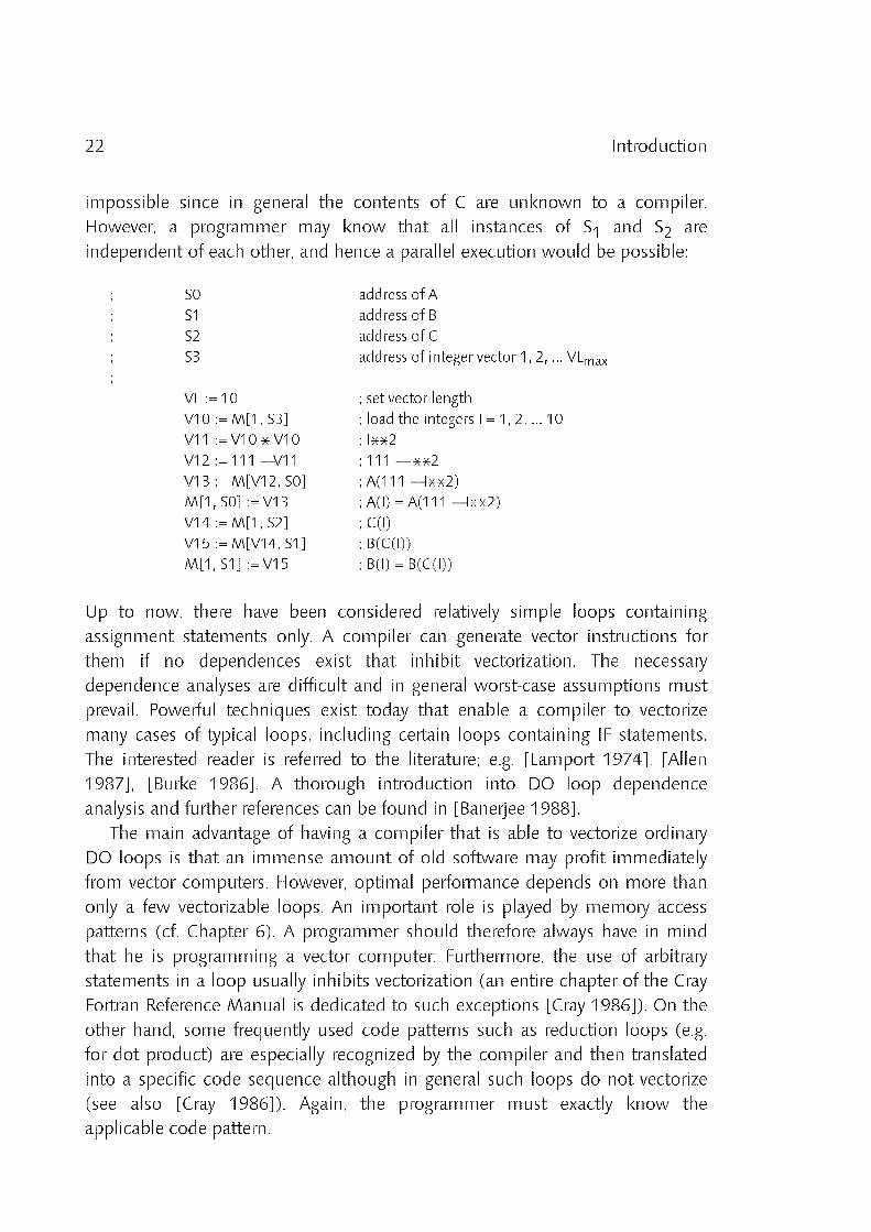
Although both index expressions I and 111 − I**2 in S1 denote disjoint sets ofindices, a compiler in general cannot recognize this situation because theright_hand expression is not linear in I. For the second statement, a compilerwould have to decide whether there are two integers i1 and i2 with i1 9 i2 and 1# i1, i2 # 10 such that i1 = C(i2) (or whether C(i) = i for all i's), which is in fact
22 Introduction
impossible since in general the contents of C are unknown to a compiler.However, a programmer may know that all instances of S1 and S2 areindependent of each other, and hence a parallel execution would be possible:
; S0 address of A
; S1 address of B
; S2 address of C
; S3 address of integer vector 1, 2, ... VLmax
;
VL := 10 ; set vector length
V10 := M[1, S3] ; load the integers I = 1, 2, ... 10
V11 := V10 * V10 ; I**2
V12 := 111 − V11 ; 111 − I**2
V13 := M[V12, S0] ; A(111 − I**2)
M[1, S0] := V13 ; A(I) = A(111 − I**2)
V14 := M[1, S2] ; C(I)
V15 := M[V14, S1] ; B(C(I))
M[1, S1] := V15 ; B(I) = B(C(I))
Up to now, there have been considered relatively simple loops containingassignment statements only. A compiler can generate vector instructions forthem if no dependences exist that inhibit vectorization. The necessarydependence analyses are difficult and in general worst_case assumptions mustprevail. Powerful techniques exist today that enable a compiler to vectorizemany cases of typical loops, including certain loops containing IF statements.The interested reader is referred to the literature; e.g. [Lamport 1974], [Allen1987], [Burke 1986]. A thorough introduction into DO loop dependenceanalysis and further references can be found in [Banerjee 1988].
The main advantage of having a compiler that is able to vectorize ordinaryDO loops is that an immense amount of old software may profit immediatelyfrom vector computers. However, optimal performance depends on more thanonly a few vectorizable loops. An important role is played by memory accesspatterns (cf. Chapter 6). A programmer should therefore always have in mindthat he is programming a vector computer. Furthermore, the use of arbitrarystatements in a loop usually inhibits vectorization (an entire chapter of the CrayFortran Reference Manual is dedicated to such exceptions [Cray 1986]). On theother hand, some frequently used code patterns such as reduction loops (e.g.for dot product) are especially recognized by the compiler and then translatedinto a specific code sequence although in general such loops do not vectorize(see also [Cray 1986]). Again, the programmer must exactly know theapplicable code pattern.

23Introduction
1.4 Vectorization of Fortran 90 Array Expressions
Fortran 90 explicitly supports array expressions, i.e. expressions where theoperands may be entire arrays [Metcalf 1987]. The involved arrays must havethe same shape, i.e. they must have the same number of dimensions andcorresponding dimensions must have the same length. Operations are thenapplied element_wise. The array expression
REAL, ARRAY (20, 30) :: A, B, C
...
A := B + C * 0.5
corresponds to the following DO loop nest (using the new Fortran 90 syntax):
DO I = 1, 20
DO J = 1, 30
A(I, J) = B(I, J) + C(I, J) * 0.5
END DO
END DO
The definition of the semantics of array expressions requires the completeevaluation of the expression on the right_hand side of an assignment before any(partial) result is assigned to the array variable on the left_hand side. Hence, thestraight_forward translation of an array expression into nested DO loops ingeneral is only correct if the array on the left_hand side is "disjoint" from allarrays in the expression on the right_hand side of the assignment (i.e. if the setsof the array elements are disjoint) or equal to those to which it is not disjoint. Ifthis condition holds, an array expression can also be translated into vectorinstructions without further dependence analysis. If this condition is notfulfilled, an auxiliary array is usually required to correctly implement the arrayassignment.
Note that the introduction of such an auxiliary array (by the compiler!) mayhave a significant impact on the efficiency of the assignment since the arraymust be allocated first (its size may not be determinable at compile time; seebelow) and after the evaluation of the entire array expression and theassignment to the auxiliary array, the auxiliary array must be copied to thedestination array of the assignment. Finally, it must be deallocated. Thus, acompiler should try to avoid its introduction whenever possible. As alreadyexplained, this decision requires a "disjoint_or_equal" test. Because not onlyentire arrays but also subarrays may be used in array expressions, this test mightnot be decidable at compile time (the subarrays might be specified byvariables). The array assignment

24 Introduction
A(1 : 100, K) = A(J : J+99, K)
can only be translated into a simple loop (and hence into vector instructions)
DO I = 1, 100
A(I, K) = A(J + I − 1, K)
END DO
if the subarrays A(1 : 100, K) and A(J : J+99, K) are disjoint or equal (in case ofoverlapping subarrays a translation into a simple loop or vector instructionsrespectively may also be possible; however, in this case the "iteration direction"may be not clear at compile time). If the value of J is unknown at compile time,a pessimistic translation using a temporary array is usually unavoidable (or arun_time check is required to select between several different code sequences).Unfortunately, the situation is even worse: in a Fortran 90 subarray specificationit is not only possible to specify a lower and an upper bound, but also a stride.For example, A(1 : 99 : 2, K) denotes the elements A(1, K), A(3, K), ... A(99, K).In this case, arrays involved in an array expression are not simply rectangularsubarrays but consist of "grid elements" of the subscripted arrays. If one of thethree components of an array subscript (begin, end, stride) is a variable, thelength of the array is unknown at compile time and must be determined at runtime (possibly involving division). The access order of the elements depends onthe sign of the stride. If the same array name occurs on both sides of an arrayassignment, the decision whether its subscripts denote disjoint or equal arrayelements may lead to diophantine equations.
Although at first sight, Fortran 90 array expressions seem to be an elegantconstruct to support vector or parallel computers, their implicit complexityrequires a significant amount of work that is similar to the amount of workrequired for the vectorization of loops. Furthermore, since most of this work ishidden from the programmer, he might not even be aware of the heavy_weighttool he is using.
1.5 Array Parameters in Fortran
In Fortran an array is always passed by reference and the programmer isresponsible for its correct usage within the subroutine. If the length of the arrayis unknown at compile time, it is passed as an additional parameter by
convention. Within the subroutine, the length parameter is then used tocorrectly define the array as a local variable. If an array is multi_dimensional,so_called leading dimensions (LDx) are passed as additional parameters. The

25Introduction
matrix multiply subroutine
SUBROUTINE MUL (A, LDA, B, LDB, C, LDC, N)
INTEGER LDA, LDB, LDC, N
REAL A(LDA, 1), B(LDB, 1), C(LDC, 1)
...
END
expects three N x N arrays A, B and C. The leading dimensions of these arraysLDA, LDB, and LDC and the size N are passed explicitly. Within the subroutine,the leading dimensions are used to declare the arrays A, B and C. In fact, this isonly a specification of the "address computation rule" for the compiler since thelength of the last dimension is often simply set to 1 (and no index checks areperformed in Fortran). A correct call of the subroutine for three 100 x 100 arraysX, Y, Z would be the following
REAL X(100, 100), Y(100, 100), Z(100, 100)
...
CALL MUL(X, 100, Y, 100, Z, 100, 100)
Since for the parameters A, B and C simply the addresses of the correspondingarrays X, Y, and Z are passed, arbitrary subarrays may be specified as arguments.The following call
CALL MUL(X(10, 20), 100, Y(30, 40), 100, Z(50, 60), 100, 10)
performs a matrix multiplication on the 10 x 10 subarrays X(10 : 19, 20 : 29),Y(30 : 39, 40 : 49) and Z(50 : 59, 60 : 69) (using the Fortran 90 notation). If theleading dimension arguments are modified, even worse tricks are possible. Notethat these "techniques" are the only methods to pass subarrays in Fortran.Therefore they must also be used in high_quality numerical applications, suchas Linpack [Dongarra et al. 1979].
Fortran 90 allows the explicit specification of subarrays as explained inSection 1.4. Within subroutines, an array parameter may be declared to assumethe size of the corresponding argument. Using a RESHAPE transformation, theshape of the array may be arbitrarily changed and then passed as an argument.However, the old_style parameter passing conventions are still valid.


2 A Language Proposal
In the previous chapter it has been argued, why conventionally usedprogramming languages such as Fortran 77 are not sufficient for the task ofprogramming vector computers. It has been concentrated on two points,namely vectorization of loops and parameter passing of subarrays. For a morethorough survey of related languages, see Chapter 4.
Two new language constructs are proposed which subsequently are shownto solve these problems. These constructs have been intergrated into anexperimental language called Oberon_V. Oberon_V evolved from Oberon whichwas chosen as a basis because it is one of the very few modern general_purposeprogramming languages which fulfill the main criteria for good languagedesign: simplicity, security, fast translation, efficient object code and readability
[Hoare 1974].In the following sections only the new language constructs are explained;
the full language report may be found in Appendix A. Section 2.3 comprises adiscussion of design decisions which lead to differences between Oberon andOberon_V. For a general introduction to Oberon the reader is referred to theliterature [Reiser 1992].
2.1 The ALL Statement
FOR loops and similar loop constructs in other languages (e.g. Fortran DOloops) explicitly describe a deterministic and sequential iteration process. Inmany cases the task to be performed is overspecified by such loop constructs.Let us consider a simple example: the task is to scale all elements of an array A.A FOR loop such as the following

28 A Language Proposal
VAR
A: ARRAY 100 OF REAL;
c: REAL;
...
FOR i := 0 TO 99 DO
A[i] := A[i] * c
END
specifies not only that each element of A be scaled with c but also in whichorder they are to be scaled. Indeed, the exact execution order does not matterin the example and thus could be non_deterministic. Furthermore, even thesequential execution of the loop is unimportant, since for each value of idifferent (and thus independent) variables are accessed. In the example, severalor all elements could also be scaled in parallel without changing the effect ofthe FOR loop.
It is interesting that the informal description of the task "multiply allelements of array A with the scale factor c" does neither specify a particular order
nor sequential execution. It is the programmer (forced by the programminglanguage he uses) who translates the task into a deterministic and sequentialprocess. Thus, inherent properties of the task are destroyed by "doing more thannecessary" during its translation into a program. In order to vectorize such aloop, a compiler has to recover these properties using dependence analysis.
One must carefully distinguish between non_deterministic and parallelexecution. If there were an imaginary FOREACH statement which would allowto express the sequential execution of a statement sequence in anon_deterministic order, it would be possible to compute the sum s of allelements of an array A by
VAR
A: ARRAY 100 OF INTEGER;
s: INTEGER;
...
s := 0;
FOREACH i IN {0 .. 99} DO
s := s + A[i]
END
since the order in which the elements are added does not matter (at least forintegers). Obviously, parallel execution would lead to a wrong result. Theimportance of having such non_deterministic language constructs has beenstressed before; they do not only allow to avoid overspecification of programsbut as a consequence also simplify program verification. Examples are thenon_deterministic evaluation of guards in Dijkstra's IF and DO statement

29A Language Proposal
[Dijkstra 1976] or the programming notation UNITY used for the developmentof parallel programs [Chandy 1988].
In Oberon_V a new structured statement called ALL statement has beenintroduced. The ALL statement is used to specify the independent execution ofa sequence of assignments for a set of (index) values within specified intervals.The assignment sequence is prefixed by a range declaration which is used tospecify these intervals or ranges. A similar construct (FORALL) may be found inVienna Fortran [Zima 1992]; a Fortran offspring especially directed towardsprogramming of parallel machines. As an introductory example let us considerthe ALL statement corresponding to the scaling example:
VAR
A: ARRAY 100 OF REAL;
c: REAL;
...
ALL r = 0 .. 99 DO
A[r] := A[r] * c (* S(r) *)
END
The range declaration r = 0 .. 99 specifies a new range identifier r which isassociated with the range 0 .. 99. Within the ALL statement, the range identifierr stands for any integer value i within its associated range, i.e. for any of theintegers 0, 1, 2, ... 99 in the example. Execution of the ALL statement meansthat the enclosed assignment sequence S(r) is executed exactly once for eachvalue i that can be assumed by the range identifier r. The order in which rassumes such a value i is undefined. Furthermore, in order to be correct, the ALLstatement requires that different assignment sequences S(i1) and S(i2) with i1 9i2 be independent of each other; i.e. that no variable accessed or modified in theassignment sequence where r = i1 is modified in any other assignmentsequence where r = i2. In the example, the variables accessed or modified byS(i1) obviously are different from the variables accessed by S(i2) for i1 9 i2, thusany two assignment sequences S(i1) and S(i2) are independent of each other.Because they are independent, they may even be executed in parallel.
In general, an ALL statement may introduce more than a single rangeidentifier. In this case, the enclosed assignment sequence is executed exactlyonce for each combination of values the range identifiers may assume and asimilar independence rule must hold. Using EBNF, the syntax of the general ALLstatement is:

30 A Language Proposal
AllStatement = ALL RangeDeclaration DO AssignmentSequence END.AssignmentSequence = [Assignment {";" Assignment}].RangeDeclaration = RangeList {"," RangeList}.RangeList = ident {"," ident} "=" Range.Range = Expression ".." Expression.
(for the definition of the non_terminal symbols Assignment and Expression aswell as the symbol ident see Appendix A). The semantics of the ALL statementcan be specified by a rule of inference (cf. Section 2.3.6) which also serves as aproof outline for verifying programs containing ALL statements. For brevity, onlythe case with a single range identifier is shown here (the general definition isagain found in Appendix A). P, Q, P(r) and Q(r) denote predicates describingthe program states before and after the execution of the ALL statement or theenclosed assignment sequence S(r), respectively:
{P} ALL r = a .. b DO S(r) END {Q}
holds if conditions P(r) and Q(r) exist, such that
(1) P ↑ (R i : a # i # b : P(i))(2) R i : a # i # b : {P(i)} S(i) {Q(i)}(3) (R i : a # i # b : Q(i)) ↑ Q
and
R i, j : (a # i, j # b) Y (i 9 j) : (in(i) G out(j) = F) Y (out(i) G out(j) = F)
with in(i) : set of variables that have been accessed by S(i)and out(i) : set of variables to which values have been assigned to by S(i)
When applied as a proof scheme to the scaling example one obtains:
{P : (R i : 0 # i # 99 : A[i] = A0[i])}
ALL r = 0 .. 99 DO
{P(r) : (A[r] = A0[r])} A[r] := A[r] * c {Q(r) : (A[r] = A0[r] * c)}
END
{Q : (R i : 0 # i # 99 : A[i] = A0[i] * c)}
It is easily verifyed that (1), (2) and (3) hold. Furthermore, all assignments areindependent since in(i) = out(i) = {A[i]} and of course

31A Language Proposal
R i, j : (0 # i, j # 99) Y (i 9 j) : {A[i]} G {A[j]} = F
Thus, the example using the ALL statement correctly implements the scaling ofarray A. Since all assignment sequences must be independent and thus can beregarded "separately", proofs for larger ALL statements are in general not muchmore complicated. Note that it is necessary to check whether independenceholds or not, as will be shown by the following counter example (in particular,independence is not implied by (1), (2) and (3)):
{P : (s = 0)}
ALL r = 0 .. 99 DO
{P(r) : (s = 0)} s := s + 1 {Q(r) : (s = 1)}
END
{Q : (s = 1)}
Obviously (1), (2) and (3) hold, but in(i) G out(j) = {s} 9 F for different i and j.Because the ALL statement may be either executed sequentially or in parallel (oreven partially sequential and partially in parallel), the result is indeed undefined.
If a particular sequential execution order were specified, an ALL statementintroducing n range identifiers
ALL r1 = a1 .. b1, r2 = a2 .. b2, ... rn = an .. bn DO
S(r1, r2, ... rn)
END
where S denotes an assignment sequence containing the range identifiers r1, r2,... rn could be implemented by a loop nest
i1 := a1;
WHILE i1 <= b1 DO
i2 := a2;
WHILE i2 <= b2 DO
...
in := an;
WHILE in <= bn DO
S(i1, i2, ... in);
INC(in)
END;
...
INC(i2)
END;
INC(i1)
END

32 A Language Proposal
Such a conversion must be understood as overspecification of a task, for whichan ALL statement would suffice. It immediately follows that the reverseconversion is wrong in general.
Due to its properties, an ALL statement can (almost) always be translatedinto vector instructions (if an assignment contains boolean operators orfunction calls, vectorization may be inhibited, see Section 3.7.2). Hence, it iseasily possible to decide, whether certain parts of a program vectorize or not.This stands in sharp contrast to the situation in Fortran.
Instead of demonstrating more elaborate examples underlining theusefulness of ALL statements for practical programs, the reader is referred toAppendix B where he may find a few longer program samples extensively usingALL statements.
2.2 Array Constructors
Oberon_V array constructors are used to construct new arrays consisting of
elements of other arrays. Note the difference between Oberon_V arrayconstructors and constructors in other languages which are used to constructarrays or records of arbitrary components (e.g. Fortran 90 array constructors[Metcalf 1987]). An Oberon_V array constructor consists of a range declarationsimilar to the one used in ALL statements, followed by an expression using therange identifiers which have been declared in the range declaration. The syntaxof the array constructor is:
ArrayConstructor = "[" RangeDeclaration ":" Expression "]".RangeDeclaration = RangeList {"," RangeList}.RangeList = ident {"," ident} "=" Range.Range = Expression ".." Expression.
(for the definition of the non_terminal symbol Expression and the symbol identthe reader is again referred to Appendix A). An Oberon_V array constructor is ofthe form
[r1 = a1 .. b1, r2 = a2 .. b2, ... rn = an .. bn: E(r1, r2, ... rn)]
where E(r1, r2, ... rn) is an expression possibly containing the range identifiers r1,r2, ... rn. Within the expression, each range identifier rk stands for any integervalue ik within the range associated to rk as in ALL statements, i.e. ik N {ak, ak +1, ... bk}. Thus, the array constructed by the array constructor denotes an (at

33A Language Proposal
least) n_dimensional array consisting of the elements E(i1, i2, ... in). Using thevariables A: ARRAY 100 OF REAL and B: ARRAY 100, 100 OF REAL, a fewexamples shall illustrate legal array constructors and the array they construct:
Array Constructor Elements of the Constructed Array Dimensions
[r = 10 .. 20: A[r]] A[10], A[11], ... A[20] 1[r = 0 .. 10: A[3*r + k]] A[k], A[3+k], A[6+k], ... A[30+k] 1[r = 0 .. LEN(B)−1: B[r, r]] Diagonal of B 1[r = 0 .. 99: B[99−r]] B[99], B[98], ... B[0] 2[r, s = 0 .. 99: B[s, r]] Transpose of B 2
[r = 10 .. 20: ABS(A[r])] ABS(A[10]), ABS(A[11]), ... ABS(A[20]) 1[r = 0 .. 9: A[r] * B[r, r]] A[0]*B[0, 0], A[1]*B[1, 1], ... A[9]*B[9, 9] 1[r = 0 .. 4: A[r] + A[r+5]] A[0]+A[5], A[1]+A[6], ... A[4]+A[9] 1[r, s = 0 .. 99: −B[r, s]] −B 2[r, s = 1 .. 10: 1/(r+s−1)] 10 x 10 Hilbert matrix 2
The first 5 examples construct array variables, since the expression following therange declaration in the array constructor consists of a designator (see AppendixA.10.3) denoting a variable. In contrast, the last 5 examples construct array
values, since the range declarations are followed by an arbitrary expressionwhich is not only a designator denoting a variable. The right_most columndenotes the number of dimensions of the constructed array (for an exactdefinition of "number of dimensions" see Appendix A.6.2). Often, the numberof range identifiers corresponds to the number of dimensions of theconstructed array; however, this is only true if the type of the expression is notan array (see 4_th example from top).
In Oberon_V, constructed array variables may be used as arguments for open
array variable parameters. In order to make them efficiently and safelyimplementable, a few restrictions must apply, e.g. the subscripts of a designatormust contain only "linear" range expressions. Thus, an array variable constructor[r = 0 .. 9: A[r*r]] is not allowed. For a justification of these restrictions seeSection 3.9; for an exact specification of array constructors and the restrictionssee Appendix A.10.5 and A10.6.
Figure 2.1 illustrates the passing of a diagonal of the array A as an argumentto the procedure Scale. Since the array constructor introduces a single rangeidentifier r and the designator A[r, r+1] denotes a (zero_dimensional) scalar
variable, the array constructor denotes a (1 + 0 =) 1_dimensional subarray
variable of A. Within the procedure Scale, this subarray is simply referred to by

34 A Language Proposal
the parameter a; element a[0] stands for A[0, 1], element a[1] stands for A[1,2] and so on.
VAR
A: ARRAY 10, 10 OF REAL;
PROCEDURE Scale (VAR a: ARRAY OF REAL; c: REAL);
BEGIN ALL i = 0 .. LEN(a) − 1 DO a[i] := a[i] * c END
END Scale;
...
Scale([r = 0 .. 8: A[r, r+1]], 3.14)
0 1 2 3 4 5 6 7 8 9
0123456789
r
r+1
0 1 2 3 4 5 6 7 8 i
Array a
Array A
Figure 2.1 Subarray Passing
Since in Oberon_V no value parameters of structured type are allowed (seeSection 2.3.4), array value constructors cannot be used as arguments in general,but only as arguments for the predefined Oberon_V functions SUM and PROD.These so_called reduction functions reduce the contents of an array to its sum orproduct respectively. They have been introduced, because they are usedfrequently (especially SUM for dot product) and because they can beimplemented much more efficiently using special code patterns than using ALLstatements and special computation tricks (cf. Chapter 6). In general, Fortrancompilers also cannot vectorize DO loops implementing reduction functions.However, they recognize some special code patterns referring to obvious scalarimplementations of SUM and PROD, and replace them by SUM and PRODrespectively [Cray 1986].
The following example illustrates the use of the SUM reduction function tocompute the matrix product of the matrices A and B with result C. For moreelaborate examples, the reader is again referred to Appendix B.
PROCEDURE Mul (VAR A, B, C: ARRAY OF ARRAY OF REAL);
VAR i, j: INTEGER;
BEGIN

35A Language Proposal
ASSERT(LEN(A, 1) = LEN(B));
i := 0;
WHILE i < LEN(A) DO j := 0;
WHILE j < LEN(B, 1) DO
C[i, j] := SUM([k = 0 .. LEN(A, 1)−1: A[i, k] * B[k, j]]);
INC(j)
END;
INC(i)
END
END Mul;
2.3 Differences between Oberon and Oberon_V
In this section a few more subtle design decision are discussed which lead todifferences between Oberon and Oberon_V. While it was felt that some featuresof Oberon are not essential for programming of numerical applications andhence were omitted to obtain a simpler design and implementation (e.g. certainbasic types and control constructs have been omitted), other changes havebeen motivated in order to "repair" minor deficiencies (e.g. the differenthandling of procedure types). The latter can be understood as a modestcriticism of Oberon. However, it is emphasized that Oberon_V must beconsidered as an experimental language, implemented mainly to prove thefeasibility of a few specific concepts. Thus, whereas Oberon has already beenused to program many applications ranging from simple text editors tocompilers and even operating systems, and thereby proved to be appropriate forthese tasks [Wirth 1988b], an equivalent suitability test for Oberon_V has notbeen performed.
2.3.1 Basic Types
Oberon provides a set of eight basic types. The numeric types constituted bythe integer and real types form an inclusion hierarchy, i.e. the smaller typeincludes the larger type:
SHORTINT M INTEGER M LONGINT M REAL M LONGREAL
Due to this hierarchy, the conversion of a smaller type into the larger type canbe automatically performed by the compiler, whereas the reverse conversion(e.g. LONGINT to INTEGER) requires the use of a type conversion function(SHORT), since the programmer has to ensure that the conversion is legal, i.e.

36 A Language Proposal
that the value of an expression of the larger type is also comprised by thesmaller type. The main reason for having several integer or real types is storageeconomy [Wirth 1990].
In general, the use of different integer or real types within a single expressionis not recommended: in such "mixed_type" expressions, determining the exactoperations performed requires a careful and toilsome analysis of the expression.Often additional LONG or SHORT functions are required to guarantee thedesired accuracy of the computation. If the type of a variable is changed to thenext smaller type (e.g. from LONGINT to INTEGER) now unnecessary SHORToperations may remain undetected and lead to wrong results. As experienceshows, such errors are difficult to locate, especially if no hard_ or softwaresupport is available (e.g. overflow or range checks).
At least for integers, the problems disappear if only a single integer type,preferably the largest one, is used. Indeed, on modern RISC computers, differentinteger types are only treated differently in the implementation as far as memoryaccesses are concerned [Brandis et al. 1992]; e.g. once a SHORTINT is loadedinto a (32_bit) register, all operations on it are essentially LONGINT operations.Thus, it would be more adequate to specify the "storage size" of a particularinteger variable instead of specifying its type to be a "smaller integer" whichthen influences all expressions where the variable is used. Since storageeconomy is only a problem when having arrays (or records) containing integercomponents, it would suffice to have a possibility to specify the size of theseinteger components. Unfortunately, a similar solution for real types would notbe appropriate, since a "long" real number cannot simply be shortened withoutloosing its numerical accuracy.
These ideas have not been pursued further. For simplicity, Oberon_Vprovides only a single integer and real type (INTEGER, REAL) but also the typeCOMPLEX. Together they form the inclusion hierarchy:
INTEGER L REAL L COMPLEX
The real and imaginary components of a complex number can be retrieved bytwo predefined functions RE and IM respectively. Conversion of real numbers tointegers is possible with the predefined functions FLOOR, CEILING and TRUNC(see Appendix A.8.2).

37A Language Proposal
2.3.2 Pointer Types
In Oberon the extension relationship defined over records is inherited by itscorresponding pointer types; i.e. if a record R1 is an extension of a record R,then also a pointer type P1 with pointer base type R1 is an extension of apointer type P pointing to R. Since a (record) type R1 extends a type R if it isequal to R or if is a direct extension of an extension of R ([Wirth 1988a], 6.3Record Types), a pointer type P with pointer base type R is an extension of anyother (!) pointer type Q with the same base type:
TYPE
P = POINTER TO R;
Q = POINTER TO R;
R = RECORD ... END;
VAR
p: P;
q: Q;
...
p := q; q := p
Since R is the (zero) extension of itself, P can be regarded as an extension of Q.Vice versa, Q can be regarded as an extension of P. Due to the assignment rulesfor type extensions, it is possible both to assign p to q and q to p, withoutneeding their types being equal. Indeed, P and Q are both extensions of eachother and therefore should be considered as being equal. On the other hand,because the extension relation is only defined over records and its associatedpointer types, the same game does not work anymore if R is an array type. Thus,the programmer is confronted with the strange fact that any two different
pointer types pointing to the same record type are de facto equal types, but ifthey would point to an array they were not.
In Oberon_V, two pointer types are defined to be equal, if their base typesare equal. Furthermore, a pointer variable of type P may be assigned to anyother pointer variable of type Q, if the base type of P is an extension of the basetype of Q. This definition eliminates the unpleasant situation explained aboveand it makes the expansion of the extension relationship to pointerssuperfluous.
In a second step, the reserved words POINTER TO have been replaced by aPascal style pointer declaration using an arrow (↑) instead. This notation mustbe understood under consideration of the typical use of pointers. In Oberon,usually a named pointer type is declared together with its (named) base type.As a matter of style, having a pointer type called P, the corresponding base type

38 A Language Proposal
identifier is built by appending some suffix, e.g. "desc". A dual convention is tocall the base type B and the associated pointer type Bptr (by appending thesuffix "ptr"). Frequently, only the pointer type is used in variable and parameterdeclarations, i.e. the name of the record type merely clutters the definition.However, type extensions require the name of the record type and thus preventthe use of anonymous record types in conjunction with a pointer typedeclaration as in P = POINTER TO RECORD next: P END.
Instead of relying on individual naming conventions, it is better tocompletely avoid the need for such conventions. Due to the Oberon_Vcompatibility rules for pointer types, it suffices to declare the pointer base typesonly. Whenever an associated pointer type is used, it is newly declared bywriting the ↑ symbol followed by the base type name. The ↑ symbol thenexplicitly emphasizes the declaration of a pointer which enhances thereadability of the program and simultaneously serves as some kind of namingconvention. Of course, the same could have been achieved using the oldPOINTER TO notation, but then declarations would have become rather lengthy.For some examples demonstrating the typical usage of the Oberon_V pointernotation, the reader is referred to Section 5.2.
2.3.3 Procedure Types
Two types designated by two identifiers T1 and T2 are identical in Oberon ifboth identifiers T1 and T2 are equal, if they are declared to be identical in a typedeclaration of the form T1 = T2 or if variables of type T1 and T2 appear in thesame identifier list of a variable, record field or formal parameter list (with theexception of open array types). This kind of type equality is usually called name
equivalence and is opposed to structure equivalence, where two types are "equal"(or at least assignment compatible) if their structures are "equal". Pascal andModula_2 are representatives for languages using name equivalence, whereas inModula_3 [Cardelli et al. 1988] structure equivalence prevails.
While name equivalence is the standard equality relationship for types inOberon, a remarkable exception exists for procedure types. Since the type of aprocedure is constituted by its parameter list, i.e. the kind, number and types ofthe parameters as well as the procedure's result type (if any), and since the typeof a procedure is not declared in an explicit type declaration but is specified bythe procedure declaration, two procedures (not procedure variables) alwayshave different types. Thus, in order to check whether a procedure can beassigned to a variable of procedure type, the structure of both types, the variableand the procedure type must be compared; i.e. structure equivalence is used. In

39A Language Proposal
some cases, this irregularity leads to compiler error messages which are hard tounderstand by a novice user not familiar with the details. The following Oberonexample illustrates some of the problems:
TYPE
T = PROCEDURE (x, y: INTEGER; VAR z: REAL);
VAR
v: T;
PROCEDURE P (x, y: INTEGER; VAR z: REAL);
PROCEDURE P1 (p: PROCEDURE (x, y: INTEGER; VAR z: REAL));
PROCEDURE P2 (p: T);
Due to structure equivalence, it is possible to assign the procedure P to thevariable v or to call P1 or P2 with P as actual parameter. However, within P1 it isnot allowed to assign the value parameter p to the variable v, since in case of avariable assignment name equivalence is used. Nevertheless, it is possible tocall P1 recursively with p (but not with v) as actual parameter, since in this caseformal and actual parameter types are identical ("by accident"). On the otherhand, within P2 it is allowed to assign p to the variable v and to call P2recursively using p (or v) as actual parameter but it is not allowed to call P1with p as parameter.
In Oberon_V structure equivalence is used whenever procedure types areinvolved; i.e. two procedure types are considered to be "equal", if correspondingparameters and the result types (if any) are equal (see Appendix A.6.5). Thus,the problems mentioned before completely disappear.
2.3.4 Structure Assignment
In contrast to Oberon, in Oberon_V no structure assignment is allowed (withthe exception of strings, see Section 2.3.5). Its omission has several reasons:
In numerical programs, structured variables typically are arrays. Copying ofarrays should be avoided, since it is a relatively costly operation. Arrayparameters are usually passed by reference. If it is still inevitable to copy anarray, the ALL statement is an appropriate and highly efficient alternative.
If a record type R is exported, not all of its fields have to be exported. Theseprivate fields are then not visible outside the declaring module. Within a clientmodule, the meaning of an assignment of two variables of type R is difficult tounderstand, if not all record fields are known. If a private field is a pointer, arecord assignment may not be useful at all, or even worse, it may destroy

40 A Language Proposal
important properties of the exported data structure. Thus, if it is necessary toassign variables of an exported record type, an appropriate copy procedure isprobably the better solution.
Structure assignment for variables would consequently demand structureassignment for parameters. Consequently, it should also be possible to specifyopen array value parameters. While in Oberon the implementation of openarray value parameters is difficult but feasible, a similar implementation forOberon_V would be much more complicated, since then it should also bepossible to use an array value constructor as argument (i.e. as actualparameter).
The occurrence of structure assignments within larger programs, e.g. acompiler, may serve as an additional measure for its importance. In theOberon_V compiler, structure assignments are rarely required, and theirreplacement by field_wise assignments or call of a copy procedure wouldimpose neither problems nor a loss of efficiency. Last but not least, it isbelieved that in language design it is a good idea to choose (textually) "small"and unobtrusive symbols to denote efficient or simple operations, whereascostly or difficult operations should be expressed by (textually) "big" andstriking language constructs. While this rule is certainly met with the symbol":=" for the assignment of unstructured types, it is not always for the assignmentof structured types.
2.3.5 Character Sequences: The Exception
Strings and character arrays, i.e. character sequences of arbitrary length, play animportant role in many programs. Reading of input (scanning) as well asproducing output can often be formulated much more elegantly if a languageprovides an appropriate set of operations defined on strings. While in Pascal[Wirth 1971] and Modula_2 [Wirth 1985a] "string handling" is rudimentarilysupported only (it is possible to assign a string to a character array), Oberonallows for direct comparison of strings and character arrays. Furthermore, thestandard function COPY relieves the assignment of incompatible characterarrays containing character sequences.
In Oberon_V character sequences are almost always treated specially:character arrays may be assigned, strings and character arrays may be directlycompared as in Oberon and strings can be used as arguments for variableparameters (see below). Within assignments of character arrays, the right_handside must be a string or a character array containing a character sequencewhich is copied to the left_hand character array of the assignment. If necessary,

41A Language Proposal
the character sequence to be copied is appropriately shortened (i.e. assignmentof character arrays has always the semantics of the predefined Oberonprocedure COPY). Since no structure assignment is allowed in Oberon_V, thespecial assignment rules for character arrays do not conflict with other rules forstructured assignments.
Because parameters of a structured type must be variable parameters inOberon_V, the assignment compatibility of string constants and character arrayscannot be used as mechanism to pass string constants as arguments to aprocedure. Again, it is exceptionally allowed to pass a string constant asargument (i.e. as actual parameter) for a variable parameter. Since variableparameters usually expect variables as arguments, the string constant is firstcopied into an anonymous variable which is then passed instead.
2.3.6 LOOP Statements Considered Harmful
Roughly speaking, the semantics of statements can be mathematically definedby means of axioms which specify assertions that must hold before and after theexecution of a particular statement (for an introduction into this topic thereader is referred to the literature, e.g. [Hoare 1969], [Dijkstra 1976] and [Gries1981]). The essential property of structured statements (i.e. statements whichare itself composed of other statements) is that their semantics can be defined"in terms of rules of interference permitting deduction of the properties of thestructured statement from the properties of its constituents" [Hoare 1973].
While such an axiomatic specification is easily possible for most structuredstatements of Oberon [Reiser 1992], it is not at all for the LOOP statement, sinceits structure is not completely defined by itself, but depends essentially on thepresence or absence and the position of corresponding EXIT statements withinthe loop. From this viewpoint, the LOOP statement cannot honestly be called"well_structured".
Within a compiler, the implementation effort for LOOP statements is higherthan for other control structures (except the CASE statement), due to thenecessity to handle corresponding EXIT statements in any nesting level.Furthermore, it has been shown that the presence of ill_structured statementssuch as LOOP and EXIT statements in a programming language significantlycomplicate the implementation of optimizing compilers [Brandis 1993].
Due to its unimportance for numerical programs and because of theconsiderations mentioned before, the LOOP statement has been omitted inOberon_V. It might be noteworthy that its replacement by WHILE loops in thesources of the Oberon_V compiler led to a more readable and therefore more

42 A Language Proposal
easily understandable program in most cases.
2.3.7 Side_Effect Free Functions
In Oberon, function procedures are ordinary procedures which return a resultvalue; a function procedure must be called within an expression and thenstands for its result. The same function procedure may be called several timeswithin an expression, possibly with the same arguments. It is usually expectedto return a value dependent on its arguments (and its environment) only. Then,in case of multiple calls of the same function procedure with the samearguments the same result value is returned.
If a function procedure produces side effects, i.e. "anything a (function)procedure has done that persists after it returns its value" [Winston 1984], thevalue of the function may not only depend on its arguments but also on its"calling position", since as a side effect, the procedure may change itsenvironment (through global variables or variable parameters). Functionprocedures producing side effects are hard to understand and theirinappropriate use can lead to unexpected results. The location of bugs due toside effects is often quite difficult and time_consuming. In general, the use ofsuch procedures must be considered as bad programming practice.
However − like all bad habits − as long as such side effects are not explicitlyforbidden, they are used. In Oberon_V, functions are not allowed to produceside effects. This is achieved by restricting assignments to local variables onlyand by prohibiting to call proper procedures within functions. Note thatvariables referred to by pointers and variable parameters are considerednon_local variables in Oberon_V. Thus, by simply inspecting the designators onthe left_hand side of assignments a compiler may check, whether therestrictions are observed or not.
A similar solution may be found in the programming language Euclid[Lampson et al. 1977], a descendant of Pascal intentionally designed for "theexpression of system programs which are to be verified". In Euclid, functionsmust not have variable parameters nor may a value be assigned to non_localvariables. Since non_local (variable) identifiers to be visible within a function orprocedure must be "imported" explicitly in Euclid, this import is simplyforbidden within functions.
In the Oberon System [Wirth 1988b], almost all side_effect free functionprocedures obey the restrictions of Oberon_V. Only a few function proceduresproduce side effects (even visible ones − e.g. a viewer is opened), and theywould probably better be written as proper procedures.

3 Implementation
Possible implementation schemes for ALL statements and array constructors areillustrated. The first two sections comprise preliminaries that are required forthe understanding of the rest of this chapter. Theorem 3.1 is a customizedversion of a more general one to be found in [Banerjee 1988] (Theorem 4.2.3,p. 52 ff.). Variable names printed in bold face (e.g. x) are used to denoten_tupels or vectors; i.e. x : (x1, x2, ... xn). Operations on vectors are appliedelement_wise; i.e. x + a : (x1 + a, x2 + a, ... xn + a), xa : (x1a, x2a, ... xna)and x + y : (x1 + y1, x2 + y2, ... xn + yn), but xWy : e xkyk (1 # k # n) where Wdenotes the dot product.
3.1 Linear Functions
A 1_dimensional linear function f(x) over the integers is a mapping of an integer xto an integer y such that y = cx, where the coefficient c is an integer, too. The setof integers dom(f) over which the function is defined, is called the domain of f,and ran(f) : {f(x) : x N dom(f)} is called its range. The set of these functions isdenoted by LF1 : {f : f(x) = cx}. A function f is called total, if dom(f) covers allintegers; and it is called partial, if it is only defined over a restricted set. In thefollowing special partial linear functions are considered, with their domainsrestricted to finite intervals of integers. To be precise, dom(f) = {x : 0 # x < l}and l > 0. The set of these partial functions is denoted by LF1(l) where l iscalled the length of f, len(f). Thus, such a function f is clearly defined by twointegers, namely its length l and the coefficient c, and therefore sometimes f =LF1(l, c) is written for the specific function f(x) = cx (0 # x < l).

44 Implementation
An n_dimensional linear function f(x1, x2, ... xn) is a mapping of n integers x1, x2,... xn to an integer y such that y = c1x1 + ... cnxn, where all the coefficients ck (1# k # n) are integers. The set of all these functions is called LFn : {f : f(x) =cWx}. The partial functions discussed in the following are restricted to rectangular
domains of the form dom(f) = {(x1, x2, ... xn) : 0 # x1 < l1, 0 # x2 < l2, ... 0 # xn< ln} or {x : 0 # x < l} for short. The set of these partial functions is denoted byLFn(l) where l is called the length of f, len(f). Thus, such a function is clearlydefined by 2n integers, namely the 2n components of l and c and sometimes f= LFn(l, c) is written for a specific function f. Linear functions may be "scaled"and "added"; i.e. the following properties hold:
LFn(l, c)a : LFn(l, ca)and LFn(l, c) + LFn(l, d) ) : LFn(l, c + d)
Sometimes it is useful to know the minimum and maximum values assumed bypartial linear functions. The positive part c+ and the negative part c− of aninteger c are defined as follows:
c+ : max(c, 0)c− : max(−c, 0)
Let f be a partial 1_dimensional linear function with len(f) = m+1, i.e. f =LF1(m+1, c):
thus 0 # x # msince c+ 3 0: 0 # c+x # c+mand −c− # 0: −c−m # −c−x # 0
After adding the last two sets of inequalities one obtains
−c−m # (c+ − c−)x # c+mc+ − c− = c: −c−m # cx # c+m (*)
i.e. ran(f) is included in the set {−c−m, −c−m + 1, ... c+m}. Indeed, −c−m andc+m are actually values of the function at the end points x = 0 and x = m ofdom(f):
if c 3 0: f(0) = 0 = −c−m f(m) = cm = c+mif c # 0: f(m) = cm = −c−m f(0) = 0 = c+m

45Implementation
Therefore, min(f) = −c−m is the minimum value and max(f) = c+m is themaximum value assumed by the function f = LF1(m+1, c).
Theorem 3.1. Let f(x) be a partial n_dimensional linear function with length l =m+1, i.e. f = LFn(m+1, c). Then
min(f) = −c−Wmand max(f) = c+Wm
Proof. Because of (*), for each k, 1 # k # n:
−ck−mk # ckxk # ck
+mk
is true and after summation over all k, 1 # k # n:
e −ck−mk # e ckxk # e ck
+mkfor short: −c−Wm # cWx # c+Wm
Again, these values are indeed assumed by f(x), since f(a) = −c−Wm and f(b) =c+Wm with a and b defined as follows:
ck 3 0: ak = 0 bk = mk (1 # k # n)ck # 0: ak = mk bk = 0 (1 # k # n)
`
3.2 Affine Functions
An n_dimensional affine function f over the integers is a mapping of n integers xto an integer y such that y = cWx + c0. The set of total affine functions is calledAFn, whereas AFn(l) denotes the set of affine functions restricted to arectangular area with l = len(f). A specific affine function f is written as f =AFn(l, c, c0); f is clearly defined by 2n+1 values. Besides "scaling" and "adding",affine functions may be "moved" and the resulting functions are still affinefunctions; i.e. the following identities hold:
AFn(l, c, c0) + a : AF n(l, c, c0 + a)and AFn(l, c, c0)a : AFn(l, ca, c0a)and AFn(l, c, c0) + AFn(l, d, d0) : AFn(l, c + d, c0 + d0)

46 Implementation
Linear functions may be regarded as a special case; i.e. LFn(l, c) = AFn(l, c, 0)and one may write LFn(l, c) = AFn(l, c, c0) − c0. Using this relationship,Theorem 3.1 is easily adapted to affine functions and then leads to
Theorem 3.2. Let f = AFn(m+1, c, c0). Then min(f) = c0 − c−Wm, and max(f) = c0+ c+Wm.
3.3 Representation of Expressions by Expression Trees
Expressions consist of operands and operators; operands are either literals (i.e.constant values), designators or expressions themselves. Operators combineone or several operands with an operation. Note: in Oberon_V there are alsosets and functions calls. Sets may be reduced to expressions consisting ofliterals and designators, whereas function calls may be thought of being treatedas special (user_defined) operators.
Expressions can be represented by expression trees. Their nodes are eitherleaf nodes representing literals or designators, or inner nodes representingoperations (Figure 3.1). Inner nodes usually have one or two successors: theiroperands. General techniques for the construction of expression trees fromtextual representations of expressions are well_known and not explained further(cf. [Aho 1977]).
op1
op2
x y
z
inner nodes
leaf nodes
expression
(x op2 y) op1 z
corresponding expression tree
Figure 3.1 Expression Trees
A designator consists of a (variable) identifier followed by selectors which againmay contain expressions, e.g. an expression i denoting the element indexwithin a designator of the form A[i]. Variable access can be regarded as
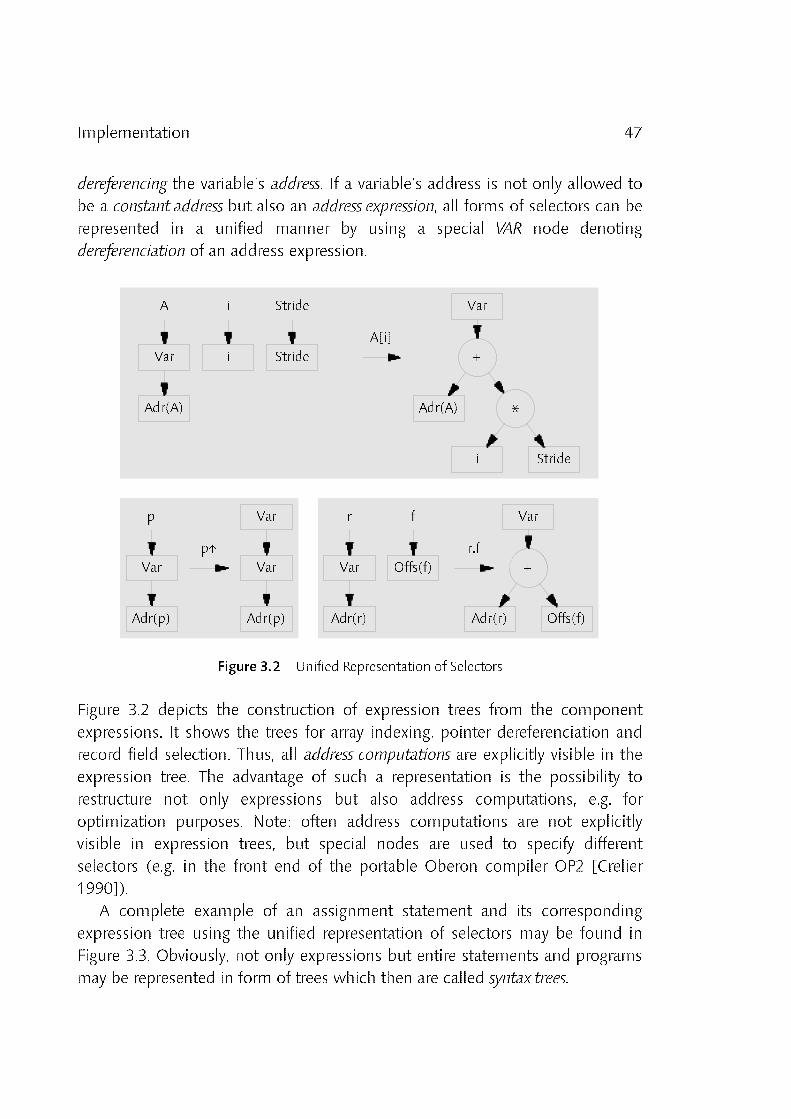
47Implementation
dereferencing the variable's address. If a variable's address is not only allowed tobe a constant address but also an address expression, all forms of selectors can berepresented in a unified manner by using a special VAR node denotingdereferenciation of an address expression.
Var
+
*
Stride
Adr(A)
i
Var
Adr(A)
i Stride
A i Stride
A[i]
Var Var
Var
Adr(p) Adr(p)
p
p↑
Var
+
Offs(f)
Offs(f)Var
r f
r.f
Adr(r)Adr(r)
Figure 3.2 Unified Representation of Selectors
Figure 3.2 depicts the construction of expression trees from the componentexpressions. It shows the trees for array indexing, pointer dereferenciation andrecord field selection. Thus, all address computations are explicitly visible in theexpression tree. The advantage of such a representation is the possibility torestructure not only expressions but also address computations, e.g. foroptimization purposes. Note: often address computations are not explicitlyvisible in expression trees, but special nodes are used to specify differentselectors (e.g. in the front end of the portable Oberon compiler OP2 [Crelier1990]).
A complete example of an assignment statement and its correspondingexpression tree using the unified representation of selectors may be found inFigure 3.3. Obviously, not only expressions but entire statements and programsmay be represented in form of trees which then are called syntax trees.

48 Implementation
+F
*F
:=
+
*
Adr(x)
Adr(y)
Adr(i)
Adr(A)
CONST
N = 100;
VAR
A: ARRAY N OF REAL;
t, x, y: REAL;
i: INTEGER;
BEGIN
...
t := A[i]*x + y
Stride
(For strides = 1 no multiplication
node is necessary)
Adr(t)
VAR
VAR
VARVAR
VAR
VAR
Figure 3.3 Syntax Tree of an Assignment
3.4 Compilation of Range Declarations
Range declarations precede assignment sequences in ALL statements as well asexpressions in array constructors. A 1_dimensional range declaration introducesa single range identifier r and associates it with a range. In the following it willbe shown that every range identifier denotes the range ran(f) of a partial affine
function f; and vice versa that ran(f) of every partial affine function f may beexpressed by a range expression, i.e. an expression containing range identifiers asoperands. This correspondence will be used to represent a range within acompiler's data structures and also explains the name range identifier.
Let r be a range identifier associated with the range a .. b; i.e. the rangestanding for the set of integers {a, a+1, ... b}. Then, for a function f = AF1(b−a+1,1, a) the range is ran(f) = {1x + a : 0 # x < b−a+1} = {a, a+1, ... b}, i.e. the rangeof the function corresponds to the range a .. b and the length of the functioncorresponds to the length of the range. Vice versa, let f be an affine functionwith f = AF1(l, c, c0). Then, the corresponding range ran(f) can be denoted bythe range expression r*c + c0, where r is a range identifier declared as r = 0 ..l−1.

49Implementation
Thus, a range r − which is also a range expression − can be identified with thecorresponding partial affine function f. Since a specific function f = AF1(l, c, c0)is clearly determined by 3 values, a range can be represented by these values.
In general, a range declaration introduces more then one range identifier. Aswill be seen in Section 3.5, computations are simplified if the correspondencebetween a single range r and a 1_dimensional affine function f is generalized ton_dimensional range declarations and functions. Let us consider the followingn_dimensional range declaration:
r1 = a1 .. b1, r2 = a2 .. b2, ... rn = an .. bn
Each range ri (1 # i # n) corresponds to a function fi N AFn by the followingrelationship (with dik denoting the Kronecker symbol, i.e. dik = 1 for i = k anddik = 0 for i 9 k):
ri = ai .. bi + fi = AFn(l, ci, ci0) with cik = dik and ci0 = ai (1 # i, k # n)
and the length l is the same for all functions fi; namely li = bi − ai + 1 (1 # i #n); i.e. each range ri is identified with an n_dimensional partial affine functionwhich "ignores" the values of all xk with i 9 k and "behaves" like in the1_dimensional case for xi. Since the length l is the same for all functions fi, itsuffices to store it only once. Each range of an n_dimensional range declarationis clearly defined by n+1 values (the n values of ci plus ci0). The followingexample illustrates the situation: the 3_dimensional range declaration
CONST
n = 10;
VAR
a, b: INTEGER;
...
u = 0 .. n−1, v = −10 .. 10, w = a .. b
declares 3 range identifiers with the associated affine functions and theircoefficients:
Function Coefficients (ci0, ci1, ci2, ci3)
fu(x) = (1, 0, 0)Wx + 0 0, 1, 0, 0fv(x) = (0, 1, 0)Wx + (−10) −10, 0, 1, 0fw(x) = (0, 0, 1)Wx + a a, 0, 0, 1

50 Implementation
In addition, there is the length l = (10, 21, b−a+1) which is simply associatedwith the entire range declaration (thus, it makes sense to speak of the length ofan n_dimensional range declaration). During compilation a range object isassociated to each range identifier. The range object simply contains thecoefficients of the corresponding affine function. Note that a range specificationmay contain variables and entire expressions; i.e. the coefficients must be heldin a suitable form, e.g. an array of expression trees (cf. Section 5.2).
Altogether, a range declaration is compiled as follows: first of all, a newidentifier scope has to be opened (by an appropriate procedure of thecompiler's symbol table manager), since range identifiers are local to theenclosing ALL statement or array constructor. Each new range identifier is theninserted in the top scope of the symbol table (and an error is raised, if the rangeidentifier has been declared already in the same scope). For each range a .. b, arange object is created which represents the function denoted by the range (i.e.which holds the n+1 coefficients), and the length corresponding to the entirerange declaration is updated. The range object is then bound to its associatedrange identifier(s). After the range declaration has been processed, a rangeobject referred to by its associated identifier can be found with a simple tablelookup. At the end of the enclosing ALL statement or array constructor thescope is closed again. Figure 3.4 shows the contents of the top scope of acompiler's symbol table after processing of the previous range declarationexample.
u v w
previous scope
top scope
scope
0 1 0 0 −10 0 1 0 a 0 0 1
identifier list
associated
range objects
coefficients
10 21 b−a+1
length vector
c c c c0 1 2 3 c c c c0 1 2 3 c c c c0 1 2 3
l l l1 2l 3
Figure 3.4 Symbol Table Contents after Processing a Range Declaration
Note that this compilation scheme automatically leads to a canonical
representation of range declarations, since every n_dimensional range declarationis reduced to a length vector l associated with the entire declaration, and a listof n range objects which may be referred to by their associated range identifiers

51Implementation
and which are represented by the coefficients of their corresponding affinefunctions. Thus, instead of an n_dimensional range declaration of the form
r1 = a1 .. b1, r2 = a2 .. b2, ... rn = an .. bn
also the canonical range declaration
r1' = 0 .. l1 − 1, r2' = 0 .. l2 − 1, ... rn' = 0 .. ln − 1
with rk = rk' + ak and lk = bk − ak + 1 (1 # k # n) may be used instead withoutloss of generality. In this case l = (l1, l2, ... ln) denotes the length of the range
declaration.
3.5 Linear Range Expressions
Range expressions are expressions which have ranges (denoted by rangeidentifiers) as operands. Each range expression must be considered within itsenvironment, i.e. within the scope of the corresponding n_dimensional rangedeclaration. Within a particular range expression, only the range identifiersintroduced by this declaration can occur.
A conventional expression may be represented by an expression tree (cf.Section 3.3) and, of course, this holds for range expressions too. Within anexpression tree, a range is represented by its associated range object which hasbeen created during the range declaration. During parsing of an expression, theexpression tree grows. Each operator applied to its operands usually leads to anew tree node denoting the operation and pointing to its operand trees. Rangeexpressions are treated in a special way when linear operations are involved (+, −and * with a scalar value): since each range denotes a function f N AFn(l) andsince this function class is closed under addition and multiplication with ascalar value, this holds for ranges too. In the example
VAR
a, b: INTEGER;
...
ALL r = a .. b DO
... r*10 + 4 ...
the range identifier r denotes a range object corresponding to the function f =AF1(b−a+1, 1, a). Therefore the expression r*10 + 4 corresponds to the function
f*10 + 4 = AF1(b−a+1, 10, a*10 + 4) (cf. Section 3.2). Thus, linear expressionsover ranges can be transformed into linear expressions over the ranges'

52 Implementation
coefficients. Figure 3.5 illustrates this transformation for the example. Thelengths of the ranges are never changed (they are not shown in the figure).Note that for each transformation a new range object must be generated (r' andr'' in Figure 3.5), because a range object may be shared by different expressiontrees.
r
a 1
a 10
10 10
a 10
4
+
*
*
*10 + 4
r' = r * 10 r'' = r * 10 + 4
c c0 1 c c0 1 c c0 1
Figure 3.5 Transformation of Range Expressions
According to the rules for affine functions (Section 3.2), the sametransformations can be performed for n > 1. The range objects declared by ann_dimensional range declaration correspond to functions f N AFn. Since alllengths and the number of dimensions of all these functions are the samewithin the scope of the range declaration, all linear operations are well_defined.Within the scope of a range declaration, the objects involved in rangeexpressions correspond either to scalar values or such functions f. Thus, if theexpression is linear, the entire expression can be represented by a single rangeobject (cf. also Section 3.8.1). Especially, also expressions of the form a0 +r1*s1 + r2*s2 + ... + rn*sn, where a0 and the sk's designate scalar values and therk's designate range identifiers (1 # k # n), can be represented by a single rangeobject. Such computations are caused implicitly when subscripting ann_dimensional array A with n ranges rk. In this case, a0 denotes the address of Aand the sk's denote the strides.
3.6 Reorganization Properties of ALL Statements
An ALL statement consists of an n_dimensional range declaration followed by asequence of assignments. In this section it will be shown that this assignmentsequence can be reorganized in such a way that the overall semantics of the

53Implementation
ALL statement is not changed, but a potentially parallel execution becomespossible. A general ALL statement containing m assignments Ak is of the form
ALL r1 = a1 .. b1, r2 = a2 .. b2, ... rn = an .. bn DO
A1(r1, r2, ... rn);
A2(r1, r2, ... rn);
...
Am(r1, r2, ... rn)
END
where each Ak(r1, r2, ... rn) may contain the range identifiers r1, r2, ... rn. Insteadof this ALL statement, its canonical form may be used without loss of generality,i.e. the range declaration may be replaced by its canonical form (cf. Section3.4). Then, the general ALL statement looks like
ALL r = 0 .. l−1 DO
A1(r);
A2(r);
...
Am(r)
END
using an informal notation where l is the length of the range_declaration (cf.Section 3.4). According to the definition of the ALL statement, a legalinterpretation of it is (using a pseudo code notation):
FOREACH i IN {x : 0 # x < l} DO
A1(i);
A2(i);
...
Am(i)
END
After numbering the elements of the set R = {x : 0 # x < l}, an explicitsequence of m*v assignments may be written instead, with v = l1*l2* ... *ln (i.e.v is the number of elements in R):
A1(i1); A2(i1); ... Am(i1); (* S(i1) *)
A1(i2); A2(i2); ... Am(i2); (* S(i2) *)
... ...
A1(iv); A2(iv); ... Am(iv) (* S(iv) *)

54 Implementation
where each ik (1 # k # v) stands for a different element of R. The definition ofALL statements requires that any two assignment sequences S(ik) and S(il) with1 # k, l # v and k 9 l be independent of each other; i.e. no variables that havebeen accessed or modified by S(ik) are modified by S(il) and vice versa. Hence,it is allowed to reorder the assignment sequence to the following form withoutchanging its effect:
A1(i1); A1(i2); ... A1(iv);
A2(i1); A2(i2); ... A2(iv);
...
Am(i1); Am(i2); ... Am(iv)
This assignment sequence is now considered at a finer level of granularity: eachassignment A(i) is of the form D(i) := E(i) where D stands for a designator andE stands for an expression; i.e. the assignment sequence can be written in theform
D1(i1) := E1(i1); D1(i2) := E1(i2); ... D1(iv) := E1(iv);
D2(i1) := E2(i1); D2(i2) := E2(i2); ... D2(iv) := E2(iv);
...
Dm(i1) := Em(i1); Dm(i2) := Em(i2); ... Dm(iv) := Em(iv)
Because functions and hence expressions are side_effect free, and due to theindependence of different assignment sequences S(ik) and S(il), it is evenpossible to use parallel assignments instead. For parallel assignments, firstly allexpressions on the right_hand side of the assignment are evaluated and thenthe results are simultaneously assigned to the corresponding variables on theleft_hand side:
D1(i1), D1(i2), ... D1(iv) := E1(i1), E1(i2), ... E1(iv);
D2(i1), D2(i2), ... D2(iv) := E2(i1), E2(i2), ... E2(iv);
...
Dm(i1), Dm(i2), ... Dm(iv) := Em(i1), Em(i2), ... Em(iv)
Note that this sequence of m parallel assignments still has the same effect asthe original ALL statement because only semantics_preserving transformationshave been applied. On a vector computer, the expressions Ek(i1), Ek(i2), ... Ek(iv)(1 # k # m) may be implemented as vector expressions on vectors of length v.Since v is relatively large in general, it may be necessary to divide the vectorsinto a sequence of shorter vectors or vector slices (cf. Section 1.2). The readermay see himself that such a division still preserves the semantics of the ALLstatement.

55Implementation
Altogether one may conclude that a sequence of independent scalarassignments enclosed in an n_dimensional ALL statement of the form
ALL r = 0 .. l−1 DO
A1(r);
A2(r);
...
Am(r)
END
can be translated into a sequence of vector assignments of the form
A1(v);
A2(v);
...
Am(v)
where v denotes the vector of the elements of R (i.e. v = (i1, i2, ... iv) and ik N R
for 1 # k # v), without changing its original effect.
3.7 Translation of ALL Statements into Vector Instructions
With the prerequisites leading the way to this section, half the work necessaryfor the translation of ALL statements is already explained. After compilation ofthe range declaration as described in Section 3.4, the assignment sequence hasto be parsed and a list of syntax trees for these assignments is built (cf. Section3.3). Due to the properties of the ALL statement (Section 3.6) these syntax treescan be regarded as a sequence of vector assignments consisting of a designatordenoting a vector on the left_hand side and a vector expression on theright_hand side of each assignment. Section 3.7.1 explains the code generationfor 1_dimensional ALL statements, i.e. ALL statements containing a1_dimensional range declaration. The techniques are generalized ton_dimensional ALL statements in Section 3.7.2. A few interesting cases such asarray accesses of the form A[B[i]] and conditional assignments are consideredin Section 3.7.3. The handling of index checks is omitted here but explained inSection 3.9.

56 Implementation
3.7.1 1_dimensional ALL Statements
In case of a 1_dimensional ALL statement, vector instructions can be generatedwithout further reorganization of the syntax tree: as for scalar expressions, theassignment list is traversed and code is generated by recursively traversing theleft_hand and right_hand side of the expression trees for each assignment (codegeneration for scalar expression trees is not explained here; the reader isreferred to standard literature on compiler construction, e.g. [Aho 1977]). Inmost cases, a variable denoting a vector is represented by a VAR node and itsaddress which is a range object (see Sections 3.3 and 3.5, special situations aredescribed in Section 3.7.3). In the 1_dimensional case, this range objectcontains two coefficients c0 and c1 only representing the vector address (Section1.1) which directly may be used to generate the necessary vector load or storeinstruction. However, since the length of vectors is usually longer then themaximum vector length VLmax of a vector register or even unknown at compiletime, the vectors have to be sliced; i.e. a loop enclosing the vector assignmentsand additional slice pointers are required (cf. Section 1.2). As an example, asimple ALL statement is considered:
:=VAR
A, B: ARRAY 1000 OF REAL;
x: REAL;
e1, e2: INTEGER;
...
ALL i = 0 .. 99 DO
A[i * e1] := B[i * e2] * x
END
e1
e2
Adr(A)
Adr(B)
Adr(x)
*
c c0 1
c c0 1
VAR
VAR
VAR
Figure 3.6 ALL Statement and Corresponding Syntax Tree
After processing the ALL statement, the syntax tree illustrated in Figure 3.6 isobtained plus the length l = 100 of the range declaration (not shown in thefigure). For a real machine with VLmax < l (or l unknown at compile time), aslicing loop is necessary and the code may then look as follows (compiled forthe hypothetical vector computer introduced in Section 1.1):

57Implementation
; S0 address of A
; S1 address of B
; S2 variable x
; S3 variable e1
; S4 variable e2
; S5 counter (introduced by the compiler)
; S6 slice pointer A↑ (introduced by the compiler)
; S7 slice pointer B↑ (introduced by the compiler)
;
S5 := 100 ; initialize counter c with range length
S6 := S0 ; initialize A↑
S7 := S1 ; initialize B↑
Loop S10 := S5 > 0 ; c > 0
jump Exit (˜S10) ; WHILE c > 0 DO
VL := S5 ; set vector length
V11 := M[S4, S7] ; B[i * e2]
V12 := S2 *F V11 ; B[i * e2] * x
M[S3, S6] := V12 ; A[i * e1] := B[i * e1] * x
S13 := VL ; get vector length of this iteration
S14 := S3 * S13 ; e1 * VL
S6 := S6 + S14 ; A↑ := A↑ + e1 * VL
S15 := S4 * S13 ; e2 * VL
S7 := S7 + S15 ; B↑ := B↑ + e2 * VL
S5 := S5 − S13 ; c := c − VL
jump Loop ; END
Exit ...
The code for the vector expression (marked by a vertical bar on the left margin)corresponds directly to the expression tree in Figure 3.6, with the onlyexception that the coefficients c0 have been replaced by auxiliary variables(namely the slice pointers A↑ and B↑). Thus, for a 1_dimensional ALL statementwhere the expression tree contains m range objects, in general m+1 additionalvariables have to be introduced by the compiler: m variables for the slicepointers and 1 variable for the loop counter. Furthermore, note that the stridesof A and B and the scaling factor x are denoted by simple variables (e1, e2 andx) in this example. In general, strides and scalar values may be arbitraryexpressions. Beacuse these scalar expressions do not change their values duringexecution of an ALL statement, they could be computed once before enteringthe slicing loop (if these expressions would change their values, differentassignment sequences of the ALL statement would not be independent). Theseoptimizations and the introduction of the slice pointers can be obtained by asimple traversal of the syntax tree corresponding to the assignment sequence.During this traversal, the following substitutions are done:

58 Implementation
1. Introduce a new (anonymous) variable v for each scalar expression Ewhich is not simple, i.e. which is not simply a literal or anunstructured variable, or which is the coefficient c0 of a range object.
2. Substitute this scalar expression E by the newly introduced variable vin the expression tree.
3. Generate an assignment statement "v := E", i.e. the correspondingsyntax tree, and append it to a special list L1 of assignments whichhave to be executed before entering the slicing loop of the ALLstatement.
4. If the substituted expression E was a c0_coefficient of a range object,then generate an assignment statement "v := v + c1*VL" and append itto a special list L2 of assignments which have to be executed at the
end of each slicing_loop iteration.
After these transformations, a 1_dimensional ALL statement can be translated tomachine code in 5 steps (if also run_time index checks are to be generated, anadditional step is necessary; cf. Section 3.9):
1. Generate code for the assignment sequence L1.2. Generate code for the slicing loop header, i.e. introduce a new counter
variable c (preferably to be held in a register), initialize it with thelength of the range and generate code to check the terminationcondition.
3. Generate code for the vector assignments by traversing the syntaxtrees.
4. Generate code for the assignment sequence L2.5. Generate code for the slicing loop end, i.e. decrement the counter
variable c by (the current value of) VL and generate a jump to thebeginning of the loop.
In case of a range with constant length not greater then VLmax, neither a slicingloop nor additional variables have to be introduced but code can be generateddirectly by traversing the expression tree. Thus, using a constant length VLmax,vector expressions can be mapped one_to_one to the machine's vectorinstructions.

59Implementation
3.7.2 n_dimensional ALL Statements
The basic insight leading to an implementation of multi_dimensional ALLstatements is that a n_dimensional ALL statement of the form
ALL r = 0 .. l−1 DO
S(r)
END
can be emulated using n loops and n additional variables x1, x2, ... xn:
x1 := l1;
WHILE x1 > 0 DO
x2 := l2;
WHILE x2 > 0 DO
...
xn := ln;
WHILE xn > 0 DO
VL := (xn − 1) MOD VLmax + 1;
ALL r' = 0 .. VL−1 DO
S'(r')
END;
xn := xn − VL
END
...
x2 := x2 − 1
END;
x1 := x1 − 1
END
The innermost loop proceeds in steps of VL with VL # VLmax. Since theenclosed ALL statement processes vectors of length VL, no slicing loop isrequired and the statement sequence S'(r') can directly be implemented usingvector instructions (cf. previous Section). Thus, the key to the implementationof n_dimensional ALL statements is the transformation of the assignmentsequence S(r) containing n different ranges r1, r2, ... rn to an assignmentsequence S'(r') using only a single range identifier r' denoting a range of lengthVL. In the following this goal is approached in a few small steps.
Within the syntax trees of an n_dimensional ALL statement, a range objectrepresents a function f N AFn(l). For each element e of the range ran(f) of such afunction, the assignment sequence within the ALL statement must be executedonce. In case of a 1_dimensional function f(x) = c1x + c0 with 0 # x < l, therange corresponds directly to the vector of elements (e) = (c0, c0 + c1, c0 + 2c1,... c0 + (l−1)c1) and hence vector instructions can be generated immediately

60 Implementation
(Section 3.7.1). In case of an n_dimensional function f(x) = cWx + c0, allelements e of ran(f) can be enumerated using n loops and n variables x1, x2, ...xn as indicated in the beginning:
x1 := l1;
WHILE x1 > 0 DO x1 := x1 − 1;
x2 := l2;
WHILE x2 > 0 DO x2 := x2 − 1;
...
xn := ln;
WHILE xn > 0 DO xn := xn − 1;
e := f(x1, x2, ... xn)
END
...
END
END
Since f is an affine function, the enumerated values e can be computedincrementally. In this case, n auxiliary variables vk are needed and the variablesxk degenerate to counter variables:
v1 := c0; x1 := l1;
WHILE x1 > 0 DO
v2 := v1; x2 := l2;
WHILE x2 > 0 DO
...
vn := vn−1; xn := ln;
WHILE xn > 0 DO
e := vn;
vn := vn + cn; xn := xn − 1
END
...
v2 := v2 + c2; x2 := x2 − 1
END;
v1 := v1 + c1; x1 := x1 − 1
END
If the innermost loop proceeds faster than in steps of 1, e.g. in steps of VL, theelements are enumerated in form of entire vectors (e) and then the followingcode is obtained (only the innermost loop is shown):

61Implementation
...
vn := vn−1; xn := ln;
WHILE xn > 0 DO
VL := (xn − 1) MOD VLmax + 1;
(e) := (vn, vn + cn, vn + 2cn, ... vn + (VL−1)cn);
vn := vn + VL*cn; xn := xn − VL
END
...
Thus, the enumeration of ran(f) for f N AFn(l) has been reduced to theenumeration of ran(f') with f'(x) = vn + cnx and f' N AF1(VL). The sametransformations can be applied to every range object within an n_dimensionalALL statement. After these transformations, every range object corresponding toa function f N AFn(l) has been substituted by a 1_dimensional range objectcorresponding to a function f' N AF1(VL). Then, for every range object r, nauxiliary variables vkr (1 # k # n) are required. For a given k, all these vkr mustbe initialized before entering the loop k and incremented by the correspondingcoefficient ckr in the loop k, thus leading to the following loop structure for theALL statement (remember the special instruction available for the computationof VL; cf. Section 1.1):
initialize all v1r; (* prolog 1 *)
x1 := l1;
WHILE x1 > 0 DO
initialize all v2r; (* prolog 2 *)
x2 := l2;
WHILE x2 > 0 DO
...
initialize all vnr; (* prolog n *);
xn := ln;
WHILE xn > 0 DO
VL := (xn − 1) MOD VLmax + 1;
ALL r' = 0 .. VL−1 DO
S'(r')
END;
increment all vnr; (* epilog n *)
xn := xn − VL
END
...
increment all v2r; (* epilog 2 *)
x2 := x2 − 1
END;
increment all v1r; (* epilog 1 *);
x1 := x1 − 1
END

62 Implementation
The range transformation algorithm is described by the pseudo code procedureSubstituteRange. It is assumed that an expression tree is represented byExpression nodes pointing to their operands. Among others, operands may berange objects represented by Range records or VAR nodes represented byVariable records (see below). Note that each coefficient r.c[k] of a range object ris again an expression tree (possibly holding a constant object only). Since VARnodes and range objects may occur at any position within an expression tree,they must be freely interchangeable. The type definitions below indicate animplementation using type extension (for implementation details, cf. Chapter 5).The goal of SubstituteRange is to substitute all range objects with n coefficientsby range objects with only two coefficients and thereby to determine thenecessary initialization and increment statements for the newly introducedvariables vkr. These statements are held in n assignment lists called Prolog[k]and Epilog[k] respectively and subsequently can be used to generate the nloops for the ALL statement.
TYPE
Expression = RECORD ... END;
Variable = RECORD (Expression) ... END;
Range = RECORD (Expression) c: ARRAY n+1 OF ↑Expression; ... END;
VAR
Prolog: ARRAY n+1 OF assignment list;
Epilog: ARRAY n+1 OF assignments list;
PROCEDURE SubstituteRange (VAR r: ↑Range);
VAR k: INTEGER; h, v: ↑Variable; pv, c: ↑Expression;
BEGIN
pv := r.c[0]; k := 1;
WHILE k <= n DO
c := r.c[k];
IF ˜Simple(c) THEN
allocate a new variable h, generate an assignment "h := c" and append it to Prolog[1];
c := h
END;
allocate new variable v;
generate an assignment "v := pv" and append it to Prolog[k];
IF k = n THEN generate an assignment "v := v + VL * c" and append it to Epilog[k]
ELSE generate an assignment "v := v + c" and append it to Epilog[k]
END;
pv := v; k := k + 1
END;
generate a new range r' with r'.c[0] := pv and r'.c[1] := c;
r := r'
END SubstituteRange;

63Implementation
SubstituteRange processes all coefficients c = r.c[k] of a range r sequentially: anew variable v is introduced (corresponding to the variables vkr) and syntaxtrees corresponding to the assignment "v := pv" and "v := v + c" are generatedand appended to the list of prolog and epilog assignments of the k_th loop. Thevariable pv is a reference to the previously introduced variable v andcorresponds to vk−1r. In case of the innermost loop (k = n), v is incremented byVL*c since vector instructions are used and hence VL elements are processed ineach loop iteration. As an optimization, coefficients c which are not simple, i.e.which are not simply constant values or variables with simple address, aresubstituted by variables h which then are initialized outside the loop nest (i.e. inProlog[1]).
SubstituteRange is easily extended such that temporary variables areintroduced for all scalar expression that are not simple (cf. Section 3.7.1). If ln isknown at compile time and ln # VLmax for an n_dimensional ALL statement, theinnermost loop is not required. Furthermore, if ln # VLmax and n = 1, no loopand also no additional variables are required (both optimizations are omitted inSubstituteRange).
In some cases, a translation of the ALL statement into scalar instructions isdesired, either because certain vector instructions are missing or because novector instructions are available at all. Then, SubstituteRange must substitute allrange objects by scalar slice pointers. The necessary modifications at the end ofthe procedure SubstituteRange are shown below:
...
generate an assignment "v := pv" and append it to Prolog[k];
generate an assignment "v := v + c" and append it to Epilog[k];
pv := v; k := k + 1
END;
r := pv
END SubstituteRange;
(and the type of the procedure parameter r must be adjusted). When generatingthe n slicing loops, of course the vector length register must not be set and theinnermost loop counter must be decremented in steps of 1.
As an example, the transformations applied to a 2_dimensional ALLstatement are considered. After compilation of the range declaration andprocessing of the enclosed assignment, the syntax tree shown in Figure 3.7 isobtained.

64 Implementation
:=
*
100 1 Adr(x)
VAR
A, B: ARRAY 100, 100 OF REAL;
a, b: INTEGER;
x: REAL;
...
ALL i = 10 .. 20, j = a .. b DO
A[i, j] := B[j, i] * x
END
Adr(A) 1000
a
+
+ 1 100+
+
*
a 100
Adr(B)
10
c c c0 1 2
c c c0 1 2
VAR VAR
VAR
Figure 3.7 Syntax Tree of an Assignment within a 2_dimensional ALL Statement
The syntax tree is traversed recursively with SubstituteRange and the2_dimensional range objects are substituted by 1_dimensional range objects.The resulting syntax tree and the prolog and epilog assignment statements areshown in Figure 3.8.
:=
*
Adr(x)1
100
Prolog Assignments
k = 1: v1 := Adr(A) + 1000 + a; w1 := Adr(B) + a*100 + 10
k = 2: v2 := v1 ; w2 := w1
Epilog Assignments
k = 1: v1 := v1 + 100; w1 := w1 + 1
k = 2: v2 := v2 + VL; w2 := w2 + VL*100v
w
2
2
VAR
VAR VARc c0 1
c c0 1
Figure 3.8 Syntax Tree after Transformation

65Implementation
The newly introduced variables required for the range object on the left_handside are called vk, the variables introduced for the range object on theright_hand side are called wk. After introducing 2 additional counter variables x1and x2, the prolog and epilog assignments as well as the transformed syntaxtree can be used directly to generate two nested loops:
v1 := Adr(A) + 1000 + a; w1 := Adr(B) + a*100 + 10; (* prolog 1 *)
x1 := 11;
WHILE x1 > 0 DO
v2 := v1; w2 := w1; (* prolog 2 *)
x2 := b − a + 1;
WHILE x2 > 0 DO
VL := (x2 − 1) MOD VLmax + 1;
ALL r = 0 .. VL−1 DO
A'[v2 + r] := B'[w2 + r] * x
END;
v2 := v2 + VL; w2 := w2 + VL*100; (* epilog 2 *)
x2 := x2 − VL
END;
v1 := v1 + 100; w1 := w1 + 1; (* epilog 1 *)
x1 := x1 − 1
END
A' and B' stand for the arrays A and B regarded as "flattened" 1_dimensionalarrays; i.e. the addresses of A' and B' correspond to the addresses of A and B,and A' and B' are of type ARRAY 100*100 OF REAL. Since the length of therange r within the enclosed ALL statement is not greater than VLmax, the ALLstatement can be directly translated into vector instructions and the followinginstruction sequence is obtained for the example:
; S0 address of A
; S1 address of B
; S2 variable a
; S3 variable b
; S4 variable x
; S5 counter x1 (introduced by the compiler)
; S6 counter x2 (introduced by the compiler)
; S7 variable v1 (introduced by the compiler)
; S8 variable v2 (introduced by the compiler)
; S9 variable w1 (introduced by the compiler)
; S10 variable w2 (introduced by the compiler)
;
S20 := 1000 + S0 ; Adr(A) + 1000
S7 := S20 + S2 ; v1 := Adr(A) + 1000 + a
S21 := 100 * S2 ; a*100

66 Implementation
S22 := S1 + S21 ; Adr(B) + a*100
S9 := 10 + S22 ; w1 := Adr(B) + a*100 + 10
S5 := 11 ; x1 := l1Loop1 S23 := S5 > 0 ; x1 > 0
jump Exit1 (˜S23) ; WHILE x1 > 0 DO
S8 := S7 ; v2 := v1S10 := S9 ; w2 := w1
S24 := S3 − S2 ; b − a
S6 := 1 + S24 ; x2 := l2 = b − a + 1
Loop2 S25 := S6 > 0 ; x2 > 0
jump Exit2 (˜S25) ; WHILE x2 > 0 DO
VL := S6 ; VL := x2V26 := M[100, S10] ; slice of B[j, i]
V27 := S4 *F V26 ; slice of B[j, i]] * x
M[1, S8] := V27 ; slice of A[i, j] := B[j, i]] * x
S28 := VL ; get vector length of this iteration
S8 := S8 + S28 ; v2 := v2 + VL
S29 := 100 * S28 ; VL*100
S10 := S10 + S29 ; w2 := w2 + VL*100
S6 := S6 − S28 ; x2 := x2 − VL
jump Loop2 ; END
Exit2 S7 := 100 + S7 ; v1 := v1 + 100
S9 := 1 + S9 ; w1 := w1 + 1
S5 := −1 + S5 ; x1 := x1 − 1
jump Loop1 ; END
Exit1 ...
3.7.3 Interesting Cases
In this section, expression trees and corresponding code sequences for threemore interesting cases are illustrated without going too much into the details.No additional complexity is introduced by these cases but only the previouslydescribed methods are consequently applied. For all examples a 1_dimensionalrange declaration introducing a range identifier r is assumed. A, B, C and Ddenote 1_dimensional real arrays of appropriate length. Coefficients aredesignated by small letters a, b, ... h. As explained in Section 3.7.2, themulti_dimensional case can always be reduced to the 1_dimensional case.
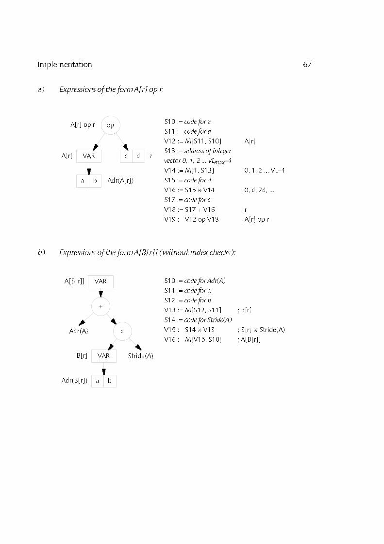
67Implementation
a) Expressions of the form A[r] op r:
r
op
Adr(A[r])
A[r]
A[r] op r
a b
c dVAR
V19 := V12 op V18 ; A[r] op r
V18 := S17 + V16 ; r
S17 := code for c
V16 := S15 * V14 ; 0, d, 2d, ...
S15 := code for d
V14 := M[1, S13] ; 0, 1, 2 ... VL−1
vector 0, 1, 2 ... VLmax−1
S13 := address of integer
V12 := M[S11, S10] ; A[r]
S11 := code for b
S10 := code for a
b) Expressions of the form A[B[r]] (without index checks):
A[B[r]]
*
+
Adr(A)
Stride(A)
Adr(B[r])
B[r]
a b
VAR
VAR
V16 := M[V15, S10] ; A[B[r]]
V15 := S14 * V13 ; B[r] * Stride(A)
S14 := code for Stride(A)
V13 := M[S12, S11] ; B[r]
S12 := code for b
S11 := code for a
S10 := code for Adr(A)

68 Implementation
c) Expressions of the form SELECT(A(r) rel B(r), C(r), D(r)):
SEL
rel
Adr(C[r]) Adr(D[r])
D[r]C[r]
Adr(A[r]) Adr(B[r])
A[r] B[r]
a b c d
e f g h
VAR VAR
VAR VAR
V23 := V19 | V22 (S16) ; SELECT(...)
V22 := M[S21, S20] ; D[r]
S21 := code for h
S20 := code for g
V19 := M[S18, S17] ; C[r]
S18 := code for f
S17 := code for e
S16 := V12 rel V15 ; A[r] rel B[r]
V15 := M[S14, S13] ; B[r]
S14 := code for d
S13 := code for c
V12 := M[S11, S10] ; A[r]
S11 := code for b
S10 := code for a
3.8 Compilation of Array Constructors
Array constructors are used to construct subarrays which subsequently may beused as arguments corresponding to open array parameters. There are twokinds of array constructors, namely constructors that specify an array variable
and constructors that specify an array value. The former may be used asarguments for variable parameters whereas the later apply as arguments for thepredefined functions SUM and PROD only.
3.8.1 Array Variable Constructors
Firstly, array constructors that specify array variables are considered which maybe used as arguments corresponding to variable parameters. Within a procedure,variable parameters stand for the variables passed as argument; i.e. they actuallyare alias identifiers for these variables. Usually variable parameters areimplemented by passing the addresses of the variables only. If a subarray is tobe passed, a descriptor specifying the addresses of the elements of the specifiedsubarray must be passed. For arbitrary subarrays, such a descriptor would be anarray containing the addresses of all the elements of the argument array:

69Implementation
VAR A: ARRAY 100 OF REAL;
...
PROCEDURE f (i: INTEGER): INTEGER;
...
PROCEDURE P (VAR a: ARRAY OF REAL; i: INTEGER);
BEGIN ... a[i] ...
END P;
...
P([i = 10 .. 19: A[f(i)]], 7)
Since f may denote an arbitrary function in the example, the descriptor to bepassed would have to contain an array consisting of the 10 addresses(Adr(A[f(10)]), Adr(A[f(11)]), ... Adr(A[f(19])). Within P, the element i couldthen be accessed by dereferencing the address i of the passed descriptor. Whilesuch an implementation would be feasible, it would probably not be desirable,due to the overhead implied by the introduction of such an address array onboth sides, the caller of P and the callee P. Thus, a simpler solution is required.
In Oberon_V, the designators which may be used within an array variableconstructor must contain linear range expressions only and no pointerdereferenciation must occur (cf. Section 3.5 and Appendix A). With thisrestrictions, passing an n_dimensional subarray requires passing an arraydescriptor containing 2n + 1 integers only as will be shown in the following.
An array variable constructor consists of an n_dimensional range declarationfollowed by a designator D denoting a variable. Without loss of generality onemay write (cf. Section 3.4):
[r = 0 .. l−1: D(r)]
The compilation proceeds as for an ALL statement without code generation (cf.Section 3.7). In a first step, the intermediate data structure is built, i.e. the rangedeclaration is compiled and an expression tree is constructed for the designatorD(r). Since all designators can be uniformly represented by VAR nodes (cf. Figure3.2) and because only linear operations are involved when subscripting an array,the expression tree generated after parsing a designator containing only linearrange expressions is simply a VAR node whose address is a range object
containing n+1 coefficients (cf. Section 3.4 and 3.5). This range objectrepresents a function f N AFn(l) where l is the length of the range declaration.
Figure 3.9 illustrates this situation for an expression tree representing anarray subscript i which is a linear range expression and thus can be representedby a range object. The construction of the expression tree proceeds asdescribed in Section 3.3, but since linear operations over ranges are

70 Implementation
transformed into linear expressions over the ranges' coefficients, the resultingtree consists of a VAR node which address is again a range object. Note thatalso the address node of an array A itself (Adr(A)) could be a range object.
A
+
Adr(A) *
Stride
c c c0 1 n
...
c0
*
c1
*
cn
...Adr(A)
StrideVAR
VAR
Stride
Stride Stride
i
A[i]Adr(A[i])
Figure 3.9 Expression Tree for a Linear Designator
According to its definition, the elements specified by the array constructor arethe elements D(i) with i N {x : 0 # x < l}. The designator D(r) is represented bya VAR node whose address is a range object. This range object specifies anaffine function f N AFn(l). For a particular i N {x : 0 # x < l}, f(i) is the address ofthe array element D(i). Thus, the addresses of all array elements D(i) are thevalues of f(i) for all i, i.e. the set ran(f) = {f(i) : 0 # i < l}. Therefore, the subarrayis clearly specified by this function f N AFn(l) which itself is specified by 2n+1integers (cf. Section 3.2), namely its n+1 coefficients − which are thecoefficients of the range object − and its length l. Apparently these 2n+1integers are the parameters to be passed to the called procedure.
In the following example a 2_dimensional subarray − a diagonal plane − of a3_dimensional array A is passed to a procedure P.
VAR A: ARRAY 10, 20, 30 OF REAL;
...
PROCEDURE P (VAR a: ARRAY OF ARRAY OF REAL);
VAR i, j: INTEGER;
BEGIN ... a[i, j] ...
...
P([u, v = 0 .. 9: A[u, 2*v, 2*v + 1])
The range declaration introduces 2 range identifiers associated with 2 affinefunctions fu, fv N AF
2(l) with l = (10, 10):

71Implementation
Function Denoted Range
fu(x) = (1, 0)Wx + 0 ran(fu) = {0, 1, ... 9}fv(x) = (0, 1)Wx + 0 ran(fv) = {0, 1, ... 9}
The designator A[u, 2*v, 2*v + 10] is translated into an expression tree in 3steps according to Section 3.4 and 3.5. In each step, the expression treeconsists of a VAR node at the root and a range object specifying a function fk NAF2(l) (it is assumed that Adr(A) = a0 and Size(A[0, 0, 0]) = 1):
Designator Associated Function
A f0 = a0 = Adr(A)A[u] f1 = (600, 0)Wx + a0 = f0 + fu * 600A[u, 2*v] f2 = (600, 60)Wx + a0 = f1 + 2*fv * 30A[u, 2*v, 2*v + 1] f3 = (600, 62)Wx + (a0 + 1) = f2 + (2*fv + 1) * 1
The subarray argument is clearly specified by f3 and l. Therefore, the values tobe passed to P are the coefficients of f3, (a0 + 1, 600, 62) and the length l =(10, 10). Within the procedure P, the address of an element a[i, j] is computedby simply applying f3 to i and j: Adr(a[i, j]) = f3(i, j). The length l is necessary forindex checks within P.
Unfortunately this translation scheme is not yet complete; there are twopoints which deserve special attention: Firstly, it must not be possible to passsubarrays that are larger than the subscripted array, i.e. some kind of index checkis required; and secondly, as will be shown below, without further restrictions itis now possible to construct subarrays which violate a major property of arrays,namely the invariant that an array of length n consists of n distinct elements. Forindex checks the reader is referred to Section 3.9. The second problem isillustrated by a small example. Let A be an array of which a subarray is to bepassed to a procedure P:
VAR
A: ARRAY 5 OF REAL;
PROCEDURE P (VAR a: ARRAY OF ARRAY OF REAL);
...
P([i = 0 .. 2, j = 0 .. 1: A[i + 2*j]])

72 Implementation
The array constructor contains a 2_dimensional range declaration with length l =(3, 2); i.e. an array containing 3*2 = 6 elements is constructed of a1_dimensional array of length 5. Since no index range is violated, two elementsof the newly constructed array must be identical! Figure 3.10 illustrates thepathological array mapping implied by the array constructor.
A[3] A[4]A[2]A[1]
A
A[0] A[2]
A[1]
A[2]
A[3]
A[4]
i
ja
A[0]
Figure 3.10 Pathological Array Mapping
Within the procedure P, both elements a[0, 1] and a[2, 0] denote the same
element A[2]! In fact, an assignment to the variable a[0, 1] would change a[2,0] too. It is easy to construct even worse situations; e.g. arrays where allelements are mapped to a single variable (using a constructor of the form [r = a.. b: v], where the range identifier r is not used within the designator v). Thus, amethod is required to detect − or better − to avoid such pathological arrays. Asexplained before, a general array constructor consisting of an n_dimensionalrange declaration and a linear designator
[r = 0 .. l−1: D(r)]
defines an affine function f N AFn(l) which specifies the mapping of the arrayindices to the corresponding element addresses. The mapping leads to apathological array if the function f is not injective, i.e. if there are two differentindices x and y with 0 # x, y < l such that both are mapped to the sameaddress. After some arithmetics one gets:
f(x) = f(y) (0 # x, y < l) Y (x 9 y)cWx + c0 = cWy + c0cWx − cWy = 0cW(x − y) = 0
with z = x − y: cWz = 0 (−l < z < l) Y (z 9 0)
73Implementation
The last equation cWz = 0 is a linear diophantine equation, i.e. a linear equation inn integer variables. The trivial solution z = 0 is not allowed, because x must bedifferent from y. Although methods exist to solve such equations (cf. [Banerjee1988]), they are not considered further, because they had to be applied at runtime in general, since the coefficients of f may be expressions containingvariables. In Oberon_V, the problem is circumvented by three additionalrestrictions which apply within array variable constructors:
1. Within a single index expression of the designator in an array variableconstructor, no two different range identifiers must occur.
2. If the array constructor contains an n_dimensional range declaration,all n range identifiers must be used at least once in the designator.
3. None of the range expressions must denote a constant value (e.g. r*0+ c, where r denotes a range, and c stands for a constant scalar value).
A linear range expression which contains no two different range identifiers is arange expression which corresponds to a function f N AFn(l) where only a singlecoefficient ck with 1 # k # n is not zero; i.e. f is a function of the form:
f(x1, x2, ... xn) = c0 + 0x1 + 0x2 + ... + ckxk + ... 0xn = c0 + ckxk
and k corresponds to the position of the range identifier in the rangedeclaration from left to right (due to the way range declarations are compiled,cf. Section 3.4). Together with restriction (3), this implies that ck must not bezero, otherwise the range expression would be constant = c0. Thus, the functionf(xk) = c0 + ckxk with ck 9 0 is injective.
In a designator of an array variable constructor, expressions can occur onlyas subscript expressions of arrays, due to the syntax of designators. Eachexpression denotes either a scalar value or it is a linear range expressioncorresponding to an injective function of the form f(xk) = c0 + ckxk. The rangeran(f) denoted by such a function f specifies the indices of the elements of thesubscripted array, and because each index occurs only once for all values of xk(0 # xk < lk), each array element is denoted only once in this array dimension.This must hold for all expressions which contain an arbitrary range identifier rk(1 # k # n) of the range declaration. Since all range identifiers must be usedbecause of restriction (2), it is not possible to denote the same array elementmore than once (if not all range identifiers would have to be used, an arrayvariable constructor of the form [u, v = 0 .. 9: A[u]] would be possible, and fordifferent v always the same element A[u] would be denoted). The situation isillustrated by means of the previous example:

74 Implementation
VAR A: ARRAY 10, 20, 30 OF REAL;
...
[u, v = 0 .. 9: A[u, 2*v, 2*v + 1]
Each expression of the designator in the array constructor contains only a singlerange identifier u or v and the functions corresponding to the range expressionsare:
Expression Function Range
u f1(x) = (1, 0)Wx + 0 ran(f1) = {0, 1, ... 9}2*v f2(x) = (0, 2)Wx + 0 ran(f2) = {0, 2, ... 18}2*v + 1 f3(x) = (0, 2)Wx + 1 ran(f3) = {1, 3, ... 19}
For all three functions only a single ck (k = 1, 2) is not zero, namely c1 in f1(because u is the first range identifier in the range declaration) and c2 in f2 andf3 (because v is the second range identifier in the range declaration). Let usconsider f3: now it is impossible that for different values of x2 the same value isassumed by f3(x1, x2). Or from the view of the range expressions: it isimpossible that the same value is assumed by the range expression 2*v + 1 fordifferent values assumed by v (note that v assumes all values within itsassociated range). Since similar conditions are fulfilled by all range expressionsand since all range identifiers are used, different array elements are denoted fordifferent values of the range identifiers u and v.
The additional restrictions impose no problems in practical applications.Even checking whether the conditions are fulfilled or not is quite easy, althoughit might not seem so at a first sight. Restriction (1) is checked whenever anarray index expression is a linear range expression: if so, the linear rangeexpression is represented by a range object, and only a single coefficient of thisrange object must not be zero. Restrictions (2) and (3) are checked aftercompilation of the array constructor: if it denotes an array variable, the subarrayis represented by a VAR node whose address is again a range object. If any ofthe coefficients ck (1 # k # n) of this range object is zero, either a rangeidentifier has not been used or the range expression where it has been used isconstant. Note that this check must be done at run time, if the coefficientexpression is not a constant.
Altogether, the compilation of an array variable constructor proceeds asfollows: the range declaration and the expression are compiled like ALLstatements. However, if an index expression occurs which is a linear rangeexpression (i.e. which is represented by a range object), restriction (1) is tested.

75Implementation
After processing the entire expression within the array constructor, theconstructor denotes a legal subarray variable if the expression is represented bya VAR node whose address is a range object; otherwise an error message israised. If any of the coefficients ck (1 # k # n) of this range object is zero, anerror message is raised. In the code generation phase, check code is generatedfor all coefficients which are not constant − they must not be zero (except c0).Then, the n+1 coefficient expressions and the n lengths are evaluated andpassed as arguments to the procedure. If the type of the designator within thearray constructor is an array too, possibly additional coefficients and lengthsmust be passed.
It might be noteworthy that in Oberon [Wirth 1988a] passing of open arraysis also permitted, however not in this general form. The main difference is thatin Oberon no explicit stride between two consecutive array elements may bespecified, as it is actually the case here: the stride in dimension k correspondsto the coefficient ck of the function f. In Oberon it suffices to pass the baseaddress of the argument array and its lengths. The strides are then computedfrom the lengths (cf. [Wirth 1992]).
3.8.2 Array Value Constructors
The use of array value constructors is restricted to arguments for the predefinedreduction functions SUM and PROD. Since these functions are known to thecompiler, inline code can be generated for them and no sophisticatedparameter passing mechanism is necessary. Thus, the problem of codegeneration for array value constructors is actually the problem of codegeneration for SUM and PROD. In the following the function SUM isconsidered only; similar considerations apply to PROD too. It is assumed thatthe summation order can be changed appropriately because addition is acommutative operation. Unfortunately, for floating_point addition this is nottrue and the result may be inaccurate especially if the operands differ largely inmagnitude. If the summation order cannot be changed for reasons of accuracy,vectorization is not possible without specialized reduction instructions. In thiscase, an ordinary loop must be used instead of SUM. A general SUM call maybe formulated as follows:
SUM([r = 0 .. l−1: E(r)])

76 Implementation
where r = 0 .. l−1 stands for an n_dimensional range declaration and E(r) for anarbitrary expression possibly containing the range identifiers r = r1, r2, ... rn.Roughly speaking, the same transformations can be applied to the expressiontree corresponding to E(r) as to syntax trees of ALL statements (cf. Section 3.7).Let us consider the following incomplete ALL statement with the same rangedeclaration r = 0 .. l−1 and the same expression E(r) like in the SUM call above:
ALL r = 0 .. l−1 DO
... := ... + E(r)
END
For an ALL statement, these transformations yield the necessary informationrequired to construct a nest of n loops. For the incomplete ALL statement thefollowing loop nest is obtained (noted in an informal manner):
loop1...
loopnset VL;
ALL r' = 0 .. VL−1 DO
... := ... + E'(r')
END
end
...
end
The ALL statement can be completed by introducing an auxiliary array S oflength VLmax:
ALL r = 0 .. VLmax−1 DO
S[r] := 0
END;
loop1...
loopnset VL;
ALL r' = 0 .. VL−1 DO
S[r'] := S[r'] + E'(r')
END
end
...
end;
s := 0; i := VLmax;
WHILE i > 0 DO i := i−1; s := s + S[i] END

77Implementation
Obviously, the execution of the n nested loops computes VL partial sums in thearray S (note that always VL # VLmax). Thus, the desired total sum s is obtainedby adding these partial sums at the end. The auxiliary array S can always beheld in a vector register, thus speeding up the computation significantly. Notethat this translation scheme relies on vector instructions that leave unusedvector elements untouched (for VL < VLmax). If the vector computer at handdoes not fulfill this requirement, a more complicated code pattern must begenerated. As an example an instruction sequence implementing the dotproduct xWy = SUM([i = 0 .. n−1: x[i] * y[i]]) for two real arrays x and y isshown:
; S0 address of x
; S1 address of y
; S2 length n
; S3 counter i (introduced by the compiler)
; S4 slice pointer x↑ (introduced by the compiler)
; S5 slice pointer y↑ (introduced by the compiler)
; V6 auxiliary vector S (introduced by the compiler)
; S7 auxiliary variable s (introduced by the compiler)
;
V6 := 0 ; initialize S
S4 := S0 ; initialize x↑
S5 := S1 ; initialize y↑
S3 := S2 ; initialize i
Loop1 S10 := S3 > 0 ; i > 0
jump Exit1 (˜S10) ; WHILE i > 0 DO
VL := S3 ; set vector length
V11 := M[1, S4] ; slice of x[i]
V12 := M[1, S5] ; slice of y[i]
V13 := V11 *F V12 ; slice of x[i] * y[i]
V6 := V6 +F V13 ; partial sum
S14 := VL ; get vector length of this iteration
S4 := S4 + S14; ; x↑ := x↑ + VL
S5 := S5 + S14; ; y↑ := y↑ + VL
S3 := S3 − S14 ; i := i − VL
jump Loop1 ; END
Exit1 S7 := 0 ; s := 0
S3 := VLmax ; i := VLmaxLoop2 S15 := S3 > 0 ; i > 0
jump Exit2 (˜S15) ; WHILE i > 0 DO
S3 := −1 + S3 ; i := i−1
S16 := V6[S3] ; S[i]
S7 := S7 +F S16 ; s := s + S[i]
jump Loop2 ; END
Exit2 ... ; result of SUM(...) in S7 (s)

78 Implementation
On a real machine, e.g. a Cray Y_MP [Cray 1988], this computation iscompletely dominated by the vector instructions (marked with a vertical bar onthe left margin). Due to its two memory ports and its independent functionalunits, two vector elements can be loaded, multiplied and added in a singleclock cycle by the Cray Y_MP. The scalar operations updating the slice pointersand the loop counter are executed "in the wake of the vector instructions"; i.e.by independent scalar functional units operating while the vector instructionsare executed. For long vectors (n 3 1000), the execution time for a dot productis approximately n clock cycles. With a cycle time of 6ns, it is possible to obtainan execution time of approximately 6ms for the dot product of two vectors oflength n = 106.
3.9 Index Checks
Index checks are required to guarantee that only array elements within theindex bounds of an array are accessed; i.e. an index expression must evaluate toa positive integer smaller than the length of the subscripted array.
For index expressions denoting a scalar value, the index check can beperformed at compile time if both the index is a constant value and the lengthof the array is known at compile time, i.e. if the array is not an open array. In allother cases, an index check must be performed at run time. With the unifiedrepresentation of designators (Section 3.3), array accesses are not directlyrecognizable anymore within the expression tree. A simple solution are explicitindex check nodes: an index check node has two operands, namely the indexexpression and the length of the array (Figure 3.11.a). The result of an indexcheck operation is the checked index. In the code generation phase of acompiler, an index check node is translated into a code sequence which raisesa trap if the index violates its index bounds (zero and the array length minusone). Figure 3.11.b shows the expression tree with index check nodecorresponding to the designator A[i].

79Implementation
Check
Index Length
+
*
StrideCheck
Length
a) Index Check Node
VAR
Adr(A)
A[i]
ib) Expression Tree for A[i]
Figure 3.11 Index Check Nodes
For index expressions that are linear range expressions, i.e. that are representedby range objects, the problem is more complicated. Since a range objectdenotes not only a single value but a set of values, a correct index check musttest whether all these values are within the allowed index bounds. Note that asimple insertion of an index check node as in the scalar case would disable thetransformation of linear expressions over ranges to linear expressions over theranges' coefficients (Section 3.5).
As explained in Section 3.4, a range object corresponds to an affine functionf N AFn(l) within the scope of an n_dimensional range declaration of length l.The range object stands for all values ran(f). Thus, if the range object is used asindex of an array with length L, all values of ran(f) must be positive and smallerthan L; i.e. the condition (0 # min(f)) Y (max(f) < L) must hold. Because f NAFn(l), using Theorem 3.2 (cf. Section 3.2) the minimum is min(f) = c0 −c−W(l−1) and max(f) = c0 + c+W(l−1). In summary, for a given range objectcontaining the coefficients c0, c1, ... cn and representing a function f N AFn(l), anindex check must assert that
(0 # min(f)) Y (max(f) < L)
with min(f) = c0 − c−W(l−1)and max(f) = c0 + c+W(l−1)
where l is the length of the range declaration and L is the length of thesubscripted array. Let us consider the following example:

80 Implementation
VAR
A: ARRAY 100 OF REAL;
...
ALL u = −4 .. 9, v = 0 .. 5, w = 10 .. 20 DO
... A[3*w − 2*v + u] ...
Within the ALL statement the array A is subscripted by a linear rangeexpression. The functions fu, fv and fw corresponding to the ranges associatedwith the range identifiers u, v and w as well as the function f corresponding tothe linear range expression are:
Function
fu(x) = (1, 0, 0)Wx + (−4)fv(x) = (0, 1, 0)Wx + 0fw(x) = (0, 0, 1)Wx + 10f(x) = (1, −2, 3)Wx + 26 ( = 3fw − 2fv + fu)
and the length vector is l = (14, 6, 11). To check whether the range expressionviolates the index bounds of the array A or not, it is necessary to computemin(f) and max(f). With c = (1, −2, 3), c0 = 26 and Theorem 3.2 the followingvalues are obtained:
min(f) = c0 − c−W(l−1) = 26 − (0, 2, 0)W(13, 5, 10) = 16max(f) = c0 + c+W(l−1) = 26 + (1, 0, 3)W(13, 5, 10) = 69
Because (0 # 16) Y (69 < 100) the index bounds are not violated by the rangeexpression. In general, this computation cannot be performed completely atcompile time, since either the coefficients ck (0 # k # n) or the lengths lk (1 # k# n) may not all be constant. However, note that partial index checks are oftenpossible, since for the computation of min(f) only the lengths lk are required forwhich the corresponding ck is negative (for positive ck's the value ck
− is zeroand also ck
−(lk−1) = 0, independent of the value of lk). A similar relationshipholds for max(f) and positive ck's.
If an index check cannot be performed completely at compile time, it shouldbe performed at run time. As illustrated in the example before, a range object isonly valid as array index, if it fulfills the constraint (0 # min(f)) Y (max(f) < L)imposed by the index check for the function f specified by the range object.Such a constraint can be represented by a constraint node associated with arange object (Figure 3.12).

81Implementation
c c c0 1 n...
r
c c c0 1 n... L
constraint noder'used as index
r
C
Figure 3.12 Range Constraints
Thus, if a range r is to be used as an index and the index check cannot beperformed completely at compile time, the range r is copied and a constraintnode C is associated with its copy r'. It is vital to copy r, because it might beshared by different expression trees (cf. Section 3.5). The constraint nodecontains a reference to the constrained range r and thus to the coefficients of thespecified function f as well as a reference to the length L of the subscriptedarray. The length l of the range declaration is known within the scope of thedeclaration and is always the same for all range objects. Hence, it is notnecessary to reference it by the constraint node.
If a range r is used within a range expression E(r), possibly producing a newrange object r', a constraint node C of r must be adopted, because the rangeobject r' representing E(r) is also valid only, if the constraint(s) of its operand rare observed. If two possibly constrained range objects r1 and r2 are added, theresulting range object r' must obey both the constraint(s) C1 of r1 and C2 of r2.Thus, a range object may be associated with an entire list of constraints to beobserved (Figure 3.13). Such constrained range objects occur only, whensubscripting arrays. As explained earlier (Section 3.5), subscripting ann_dimensional array A with n ranges r1, r2, ... rn, A[r1, r2, ... rn], implicitly leads toan expression e = a0 + r1*s1 + r2*s2 + rn*sn where a0 is the address of A andthe sk's denote the strides in dimension k. Assumed that index checks cannotbe performed at compile time, for each index rk a new constraint node Ck isgenerated. Adding all terms of the expression e leads again to a range object,and this range object is associated with the list of all these constraint nodes Ck(1 # k # n). Note that also constraint nodes must be copied sometimes,because they may be shared by different range objects: in Figure 3.13 theconstraint node C1 must be copied (C1') for the constraint list of r', whereas theconstraint node C2 may be shared.

82 Implementation
L L
r r1 2
C C1 2
1 2
L1 L2
r' = r + r1 2
C2C '1
addition
Figure 3.13 Addition of Constrained Ranges
Thus, after processing an ALL statement or an array constructor, each rangeobject within the expression tree(s) may have a list of constraint nodesassociated with it which denote the range constraints to be observed. In case ofan ALL statement, all these constraint nodes are simply collected during thetraversal of the ALL statement (e.g. as a first step in the SubstituteRangeprocedure, cf. Section 3.7.2) and held in an additional list of constraint nodesassociated with the ALL statement. In the code generation phase, first indexcheck code is generated for each of these constraint nodes (using Theorem3.2). Then code is generated for the ALL statement, as explained in Section 3.7.Note that this approach is not correct if array elements are accessed undercertain conditions only, e.g. in conditional expressions. In this case noconstraint node must be associated with the range object in question but anindex check node is introduced instead. Since no vector instructions but scalarcode only can be generated for conditional expressions containing and and or
operations, the index check node also can be translated conventionally. Thearguments of the predefined function SELECT are always evaluatedunconditionally.
In case of a legal array variable constructor, only a single range objectremains after processing the array constructor. If this range object isconstrained, in the code generation phase first index check code is generatedfor the constraints, and then parameter passing code is emitted as explained inSection 3.8.

4 Related Work
This chapter comprises a survey of other programming languages which areespecially concerned with array handling or vector processing. This survey mustnecessarily be incomplete and merely should give some idea of otherapproaches but is not intended to cover these languages in detail. Fortran 77and Fortran 90 are not mentioned here, they have been discussed in Chapter 1.
CFD. In order to make better use of the Illiac IV hardware, the programminglanguage CFD was developed at NASA Ames Research Center [Stevens 1975].CFD allows the programmer to fully control the underlying features of thehardware. No specific attempt was made to keep the language machineindependent. The language itself strongly resembles Fortran but providesspecific vector operations driving the 64 processing elements (PE) of the IlliacIV. Expressions are translated to PE instructions which operate on 64 elementseven if only scalar values are involved. Thus, the programmer is forced to "thinkparallel" if maximal performance is desired. Two compilers were built, onetranslating CFD into relocatable machine code for the Illiac IV and onetranslating CFD into Fortran. CFD is one of the first languages designedexplicitly for array processors. From the programmer's point of view, CFDprovides operations on vectors that always have length 64. Operations onlonger vectors have to be coded manually. With respect to this, CFD iscomparable to SL/1 (see below).
IVTRAN. IVTRAN is an extension of Fortran designed for the Illiac IV computer[Erickson 1975]. Normally IVTRAN programs are produced by the Fortrancompiling system for the Illiac IV [Millstein 1975] and hence serve as a kind ofintermediate program representation during Fortran compilation. IVTRAN

84 Related Work
contains all features of "standard Fortran" (i.e. an amalgam of IBM and CDCFortrans in 1975) and a few extensions in order to efficiently use the features ofthe underlying hardware. The DO FOR ALL statement is used to specify paralleloperations on array elements. For example, using DO FOR ALL the followingstatements compute the square roots of the absolute values of all elements of a3 x 7 x 10 array A:
DO 10 FOR ALL (I, J, K) / [1 ... 3] .C. [1 ... 7] .C. [1 ... 10]
IF (A(I, J, K) .LT. 0.0) A(I, J, K) = −A(I, J, K)
A(I, J, K) = SQRT(A(I, J, K))
10 CONTINUE
Assignment statements enclosed within DO FOR ALL statements are executedin parallel for all values specified by the index set. The index set is the set of alln_tuples of integers specified in the header of the DO FOR ALL statement (inour example the index set comprises the 3_tupels (I, J, K) with I N {1, 2, 3}, J N{1, 2, ... 7} and K N {1, 2, ... 10}). This stands in contrast to Oberon_V, where theassignments enclosed in ALL statements may be executed in parallel but arenot required to do so.
The Illiac Fortran compiling system comprises three sections: the "paralyzer",the compiler and a support package. The paralyzer analyzes conventionalFortran programs and tries to reveal potential parallelism by inspecting theinnermost DO loops. As a result an IVTRAN program is produced using thespecial IVTRAN features if possible. In a next step the IVTRAN program iscompiled in a rather traditional fashion and Illiac object files are generated.IVTRAN is the ancestor of many of todays Fortran dialects which are enrichedby new features in order to give the programmer the possibility to specifyparallelism in programs.
Vienna Fortran. Vienna Fortran [Zima et. al. 1992] is an experimental extensionof Fortran 77 [Brainerd 1978] oriented towards the programming of massivelyparallel machines with distributed memory. One of the main problems occuringwhen programming such machines is the distribution of arrays to differentprocessing nodes. Vienna Fortran provides special mechanisms to describesuch array layouts and to compute the addresses of the processing nodeswhich hold particular array elements or subarrays. Despite the conventionalFortran 77 statements and some Fortran 90 extensions [Metcalf 1987], ViennaFortran provides a FORALL loop which is similar to the ALL statement inOberon_V. A FORALL loop "allows the user to assert that different instantiationsof the loop body are independent and can be logically executed in parallel"; theindependence is not checked by the compiler. On a multi_processor

85Related Work
architecture, each "iteration" of the loop can be executed on another processor.Since the execution of a loop iteration must not change any data items used byanother iteration, all non_local data used by a particular iteration can begathered before the start of the iteration. Similarly, non_local data itemscomputed in a particular iteration can be communicated back to otherprocessors after the end of the iteration. This allows the compiler to optimizethe communication overhead required for the loop. Thus, the emphasis lies inthe parallelization of statements by distribution. Currently the language is stillunder development and only research compilers are available.
APL. The programming language APL, sometimes also called "Iverson Notation"is based on the work of K. E. Iverson [Iverson 1962]. APL is a highly conciselanguage designed to deal with arrays which are the only data structureavailable (some newer APL implementations also provide other data structureslike packages [Berry 1979]). Scalar values are considered as arrays with rank(dimension) zero. APL programs consist of a sequence of expressions and somekind of computed goto's; assignment statements are considered as expressions.Expressions have arrays as operands and evaluate to arrays. By defining newfunctions, a program may be structured.
APL is famous for its powerful built_in functions and operators which aredenoted by special characters. All functions are at most dyadic and alwaysright_associative. There are scalar functions and non_scalar functions: the formerare defined on scalar arguments and operate element_wise when applied toarrays, the latter are defined on arrays only. The right_hand side of anassignment is always evaluated first and then assigned to the variable on theleft_hand side. Derived functions may be built by using (built_in) functions asarguments of operators. Function arguments are also arrays. In order to pass asubarray, an appropriate function is used to retrieve the desired subarray whichis then passed as argument (which requires to copy the array in general).
APL is defined considerably concise and highly consistent both syntacticallyand semantically. Certain implementations use mathematical properties of APLexpressions in order to speed up execution [Abrams 1970]. APL was the firsthigh_level language for array processing and had a significant impact on otherlanguages and systems. The new Fortran standard Fortran_90 [Metcalf 1987]adopts the idea of applying scalar operations element_wise on arrays. TheMatlab system [MathWorks 1987] is an interactive system that pursues quite asimilar philosophy (while using a more conventional syntax). For non_arrayoriented applications however it seems difficult to use APL: expressions areprobably too powerful but on the other hand control structures are missing.Furthermore, if no restrictions are applied, APL cannot be compiled completely

86 Related Work
(because of a special function which interprets a string argument at run_time)and hence an interpreter is required.
Glypnir. Glypnir is a programming language developed at the University ofIllinois at Urbana_Champaign for the Illiac IV computer [Lawrie 1975]. Exceptthat Glypnir's syntax is Algol_based, it is similar to CFD (see Section 4.1). Inorder to obtain code which is as efficient as possible, it was decided not to hidethe machine architecture to the programmer but to provide full control over thehardware. The machine architecture is mainly reflected in two categories ofvariables, namely "CU variables" and "PE variables". The former hold scalarvalues which are to be manipulated by the Control Unit of the Illiac IV. Thelatter denote vectors or "swords" containing 64 elements to be processed byone of the 64 Processing Elements of the machine. Thus, expressionscontaining PE variables denote expression on vectors of length 64. Operationson longer vectors must be translated manually into a sequence of operations onswords. Glypnir is block structured and each block may have its own localstorage. Subroutines resemble Algol procedures but they cannot be recursiveand their arguments are called by value.
SL/1. The programming language SL/1 was developed at NASA LangleyResearch Center for the CDC Star_100 computer [Basili 1975]. The design of thelanguage was determined by a few strong design goals: the language should beas small as possible, it should be easy to implement in order to be able todevelop a compiler with minimal effort, it should force the user to expressalgorithms such that the hardware is used efficiently, and it should beextensible if necessary. As a consequence, the basic data types available in SL/1can be mapped directly to the underlying hardware and most languageoperations can be implemented by a single machine instruction of the Star_100computer. Beside of the scalar types (short) real, (short) integer and logical thecorresponding vector types (short) real vector, (short) integer vector and logical
vector were defined and considered as arrays consisting of a fixed number ofelements of the specified scalar type. The only structured type which can bedefined by the programmer is the (multi_dimensional) array, with the restrictionthat each element must be a vector or a string (a vector of dynamic length). Theset of available operators is considerably large and consists of almost alloperations that can be translated directly into a single machine instruction pluswhatever is necessary to handle SL/1 data types. As far as possible singlecharacter symbols were chosen for operators. The fact that the Star_100hardware offers an instruction to store elements of a vector depending on bitsof a bit vector lead to a tryadic assignment statement:

87Related Work
(C, Z) := A + B
where C is the result vector and Z a bit vector controlling the assignment ofindividual vector elements. The available control structures in SL/1 are moreconventional and include the WHILE, REPEAT, CASE, IF and FOR statement. Theapproach used in the design of SL/1 is quite radical and leads to a languagethat is inherently hardware dependent. In some sense SL/1 can be regarded ashigh_level assembler language.
Actus. The programming language Actus [Perrott 1979, 1983] is an offspring ofthe Pascal language family [Wirth 1971]. Actus is one of the first modernlanguages explicitly designed to ease array and vector processing. The keyconcept of the language is the notion of the extent of parallelism (eop): Witheach data structure based on an array and to most of the control structures aneop is associated. The eop denotes the set of array indices for which operationsare to be applied in parallel. If a set of array elements is going to be processedin parallel, this must already be stated in the array declaration. For example, thevariable declaration
VAR
A: ARRAY [1 : 100, 1 .. 100] OF REAL;
introduces a matrix for which every column may be accessed in parallel, i.e.which has a (maximum) eop of 1:100. In the declaration the dimension inwhich the elements may be accessed in parallel is denoted with a colon; forsome technical reason this is only possible for a single dimension. In general,A[1 : 100, j] will access the complete j_th column of this array, and A[i, 1 : 100]will access the complete i_th row. Such a column or row is then called a parallel
array. All arithmetic operators are extended such that they accept scalar valuesbut also parallel arrays; e.g. to scale all elements of the j_th column by a scalarvalue c the following expression is used
A[1 .. 100, j] * c
Obviously, the number of elements denoted by the two operands must be thesame (with exception of scalar operands) otherwise an error occurs.Furthermore it is necessary that the eop's match. For example, the expression
A[1 .. 10, i] + A[2 .. 11, j]

88 Related Work
is defined to be incorrect and must be rewritten to
A[1 .. 10, i] + A[1 .. 10 shift 1, j]
Two allignment operators shift and rotate are provided to handle this problem.Furthermore it is possible to declare index sets (to be used subsequently assubscripts for parallel arrays) and parallel constants similar to parallel arrays.
When a parallel array is used within a statement, the extent of parallelism ofthe array implicitly denotes the eop of the statement. Using the withinstatement, it is possible to specify the eop explicitly for an entire statementsequence. A hash mark (#) is used to denote the eop:
WITHIN 1 : 100 DO
BEGIN
A[#, i] := A[#, j] * c
END
In case of an assignment statement, the expression on the right_hand side isevaluated and assigned in parallel for all array elements specified by the eop.The required dependence analysis is simplified by the conditions required forthe eop's and the information provided by the shift and rotate operators. Somestatements set the eop implicitly, for example the IF statement:
IF A[1 : 10, i] > 0 THEN A[#, i] := 0
ELSE A[#, i] := 1
The guard of the IF statement is evaluated and yields a set of indices for whichthe guard is true. This set is then used as the eop for the statements in theTHEN part. The set of indices for which the guard yields false is used as the eopin the ELSE part. Similar rules are used for other control structures.
Parameter passing is extended such that it is possible to pass conformant
arrays: the array bounds of formal parameters need not be known at compiletime but are set at run time when passing the actual parameters. For example, aprocedure P with heading
PROCEDURE P (VAR a: ARRAY [beg .. end, extent] OF REAL);
expects a two_dimensional (sub_)array argument. The identifiers beg and end
take on the values of the first and last index in the first dimension of the passedarray while extent takes on the eop of the second dimension (i.e. the rows ofthe passed array must be accessible as parallel arrays). The result type of afunction may be a 1_dimensional array.

89Related Work
In contrast to Actus, in Oberon_V only independence of (assignment)statements can be expressed. This independence property allows for parallelexecution but does not require it. In Actus, processing parallel data requiresparallel execution or at least emulation of it.
Matlab. Matlab is "a high_performance interactive software package for scientificand engineering numeric computation" [MathWorks 1987]. Matlab (whichstands for matrix laboratory) was originally written to provide easy access tomatrix software packages such as Linpack [Dongarra 1979]. It evolved overseveral years and has become a standard tool in many areas. Matlab is aninteractive system and its basic data structure is − as in APL − the array.Matrices may be entered and used directly in expressions without any form ofdeclaration; hence Matlab acts like a desk calculator and is perfectly suited forexperimenting. Powerful matrix decomposition algorithms are directlyaccessible by builtin functions. For example, the following statements computethe LU factorization of a 3x3 matrix A, assign its inverse A−1 to X and calculateits determinant in D (no output is shown here):
A = [1 2 3; 4 5 6; 7 8 9]
[L, U] = lu(A)
X = inv(A)
d = det(A)
Conventional control flow statements (such as a FOR statement) make Matlaba high_level matrix language. Using script and function files a program can bestructured.


5 An Oberon_V Compiler
A compiler for a new language L serves both as a proof that an implementationof the language is feasible and as a tool for practical applications of L andhence the exploration of its usefulness. To be useful or real [Cardelli 1989], alanguage L should be theoretically and practically complete. While the formercondition can be expressed as Turing completeness, i.e. the ability of thelanguage to express every computable function, the latter condition is harder toquantify. Due to Cardelli, practical completeness is "the ability of a language toconveniently express its own (a) interpreter; (b) translator; (c) run_time support;(d) operating system". Since Oberon_V essentially provides the same featureslike Oberon [Wirth 1988a], and Oberon has been used to implement itssupporting Oberon System [Wirth 1988b], it should be possible to fulfil evencriterion (d) by Oberon_V. However, currently only a minimal form of run_timesupport has been implemented using Oberon_V.
The Oberon_V compiling system consists of the compiler OV, an object_filedecoder and an interface browser. OV is a cross_compiler for the Cray Y_MPwritten in Oberon. It runs under the Oberon System and generates relocatableCray object files. The decoder − a necessary prerequisite for a compiler writerembarking on the implementation of a back_end for a new target architecture −allows inspecting ordinary Cray object files. A dual role is played by the browser,which is used to extract interface descriptions à la Modula_2 [Wirth 1985] outof compiler generated symbol files (cf. Section 5.2.5). The browser was inspiredby a similar tool in the Oberon System and proved to be quite helpful forprogramming [Templ 1989].
In this chapter the general outline of the OV compiler is described. Section5.1 explains the module structure of the compiler. In Section 5.2 theintermediate data structure produced by the front_end is presented in detail. A

92 An Oberon_V Compiler
rough survey of the internals of the back_end is given in Section 5.3. Finally,Section 5.4 summarizes the main trouble spots of the Cray Y_MP instruction set.Oberon program extracts have been translated to Obreon_V.
5.1 Modularization
The Oberon_V compiler is a two_phase compiler. In the first phase the sourcetext is analyzed by a recursive_descent parser, and an intermediate datastructure − a symbol table and associated syntax trees − representing theprogram is built. In the second phase the intermediate data structure istraversed and code is generated. Two disjoint sets of modules can be assignedto each phase: the front_end implements the first phase and is designed to bemachine independent, whereas the low_level code generator is constituted bythe back_end modules which are machine dependent by their very nature. Bothparts are held together by the module OV which implements the user interfacerepresented by a single command called OV.Compile. OV calls the front_end andpasses the generated intermediate data structure, which is the only parameter,to the back_end. Since the front_end is machine independent, it may also beused either as a stand_alone application, e.g. for syntax and type checking ofOberon_V modules, or as a basis for other back_ends.
A portable Oberon_2 compiler (OP2) with a similar structure has been builtbefore [Crelier 1990]. However, only relatively simple parts of the front_endcould be reused for Oberon_V, namely the scanner and the parser. Due todifferences in the language and a lower level of abstraction used in theintermediate data structure of the Oberon_V compiler, many parts had to berewritten. Hence, it was decided to construct a new compiler from scratch;thereby applying the experience gained with OP2. Nevertheless, the overallstructure of the two compilers OP2 and OV is much the same, with a notableexception: no machine_level virtual code is generated by OP2 (see below).

93An Oberon_V Compiler
Virtual CodeOVV
ExpressionsOVE
Code GeneratorOVC
Object FilesOVO
OVCommands
OVT
ParserOVP
ScannerOVS
Table Handler
Back_EndFront_End
Compiler
Operating SystemFiles, Texts, Oberon
Figure 5.1 Modularization
Figure 5.1 illustrates the structure of the compiler, with the modules orderedaccording to their abstraction from bottom to top (with the highest abstractionon top) and separated into front_end and back_end.
A short description shall give a rough idea of the translation process of anOberon_V program: A source text to be compiled is decomposed into asequence of lexical units, called symbols or tokens, by means of the scannerOVS. The syntactic structure of the token stream is analyzed by the parser OVPwhich also builds the intermediate data structure. The required data types andprocedures are provided by the table handler OVT. OVT acts also as an interfacebetween front_end and back_end and hence is the only module that is importedby almost all other modules. When the source text has been analyzed withoutdetecting any errors, the generated data structure is passed to the codegenerator OVC. OVC traverses the data structure and generates virtual code for avirtual machine by means of the procedures provided by OVE. This virtual code,handled by the module OVV, allows for some optimizations, namely common
subexpression elimination and instruction scheduling. The virtual code is thentranslated into Cray machine code. Finally, the object code and some tablesholding information for the linker are assembled and a relocatable Cray objectfile is generated (OVO).

94 An Oberon_V Compiler
5.2 Intermediate Program Representation
The main task of the front_end is to generate an intermediate programrepresentation of a compilation unit. This intermediate data structure providesthe basis for all the transformations explained in Chapter 3. In the following, itis not explained how this data structure is built from a textual representation ofa program, but it is assumed that the reader is familiar with the standardtechniques for scanning and parsing a program text according to its defininggrammar (see e.g. [Wirth 1992], Chap. 12). It remains to say that the front_endmodule OVP is a simple recursive descent parser, which constructs theintermediate data structure by means of the procedures provided by moduleOVT.
The intermediate data structure consists of the symbol table information andassociated syntax trees representing statement sequences of procedure andmodule bodies. The symbol table represents all declarations, i.e. all identifiersand their associated objects (cf. Section 5.2.1). Identifiers are only visible withintheir scopes. Since scopes are properly nested in Oberon_V, they are bestmanaged using a stack. During parsing, the visible identifiers can be found bysearching the scope stack, starting with the top scope. Using Oberon_V, theprimary data structures and operations of the table handler OVT are describedby the following definitions:
TYPE
Scope = RECORD
prev: ↑Scope;
first: ↑Ident
END;
Ident = RECORD
next: ↑Ident;
name: ARRAY 32 OF CHAR;
exported: BOOLEAN;
bound: ↑Object;
usage: INTEGER (* usage = 0 <=> not used *)
END;
VAR
universe: ↑Scope;
PROCEDURE NewScope (VAR scope: ↑Scope; prev: ↑Scope);
PROCEDURE Insert (scope: ↑Scope; VAR name: ARRAY OF CHAR; VAR id: ↑Ident);
PROCEDURE This (scope: ↑Scope; VAR name: ARRAY OF CHAR): ↑Ident;

95An Oberon_V Compiler
New scopes are generated by means of the procedure NewScope; the argumentprev denoting the previous scope allows to build a stack of scopes. For everymodule, procedure, record or range declaration a new scope is opened. Forsimplicity all identifiers are held in a linear list of Ident nodes within a scope.With Insert a new identifier is appended to this list, and at the same time it ischecked whether the identifier has been declared before in the same scope(and if so, an error message is raised). Each Ident node contains informationabout the next identifier in the list, the identifier name, whether this name beexported or not and which object is associated with or bound to the identifier. Ifan identifier is used to refer to a particular object, the identifier node and hencethe associated object are retrieved using the This function. The universe scope isused as the predecessor of all module scopes; it contains a collection ofpredefined objects.
The usage field provides a simple heuristic measure for the dynamic frequency
of usage of an identifier and may be used to allocate frequently accessedvariables in registers (cf. Section 5.3.1). Whenever an identifier is used in theprogram text, its usage field is incremented taking the current nesting level ofits surrounding loops into account (and also IF, CASE and ALL statements). Thevalue zero indicates that the corresponding identifier has not been used at allwithin its defining procedure or module.
5.2.1 Representation of Objects
In Oberon_V there are constant, type, variable, procedure and rangedeclarations. In each declaration an appropriate object is introduced andassociated with an identifier. These special objects are naturally expressed astype extensions of the base type Object. In contrast to some Oberon compilers,where only a single object type is used to represent a similar variety of objects,i.e. where the information of all kinds of objects is "flattened" and packed into asingle record type [Wirth 1992][Crelier 1990], using type extensions has theadvantage of being more readable and secure. The additional assertions (typeguards) required in the compiler source provide valuable information for theprogrammer who is interested in the correctness of the implementation, butthey do not seem to slow down execution significantly. It is convenient tointroduce a few additional objects, namely objects representing parameters,record fields, predefined (standard) procedures and modules (Address andRange objects as well as Stat nodes are introduced later). All objects have a type(typ) associated with them, since Oberon_V is a strongly typed language (cf.Section 5.2.2).
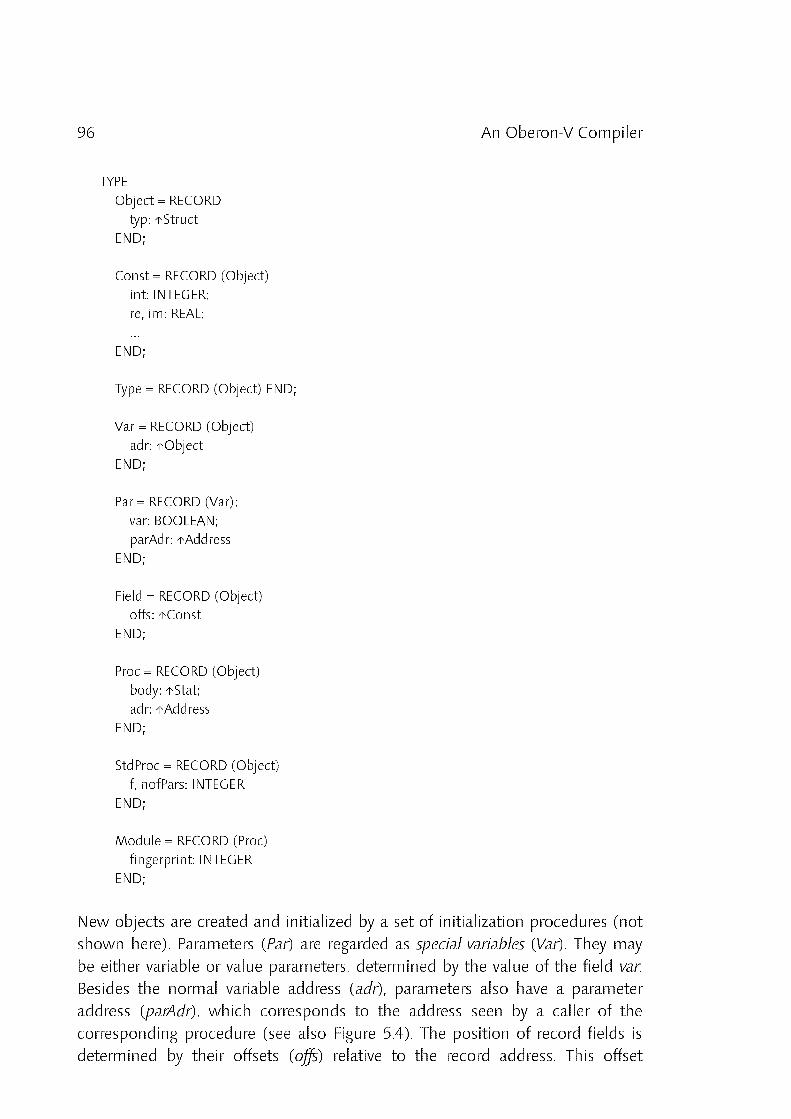
96 An Oberon_V Compiler
TYPE
Object = RECORD
typ: ↑Struct
END;
Const = RECORD (Object)
int: INTEGER;
re, im: REAL;
...
END;
Type = RECORD (Object) END;
Var = RECORD (Object)
adr: ↑Object
END;
Par = RECORD (Var);
var: BOOLEAN;
parAdr: ↑Address
END;
Field = RECORD (Object)
offs: ↑Const
END;
Proc = RECORD (Object)
body: ↑Stat;
adr: ↑Address
END;
StdProc = RECORD (Object)
f, nofPars: INTEGER
END;
Module = RECORD (Proc)
fingerprint: INTEGER
END;
New objects are created and initialized by a set of initialization procedures (notshown here). Parameters (Par) are regarded as special variables (Var). They maybe either variable or value parameters, determined by the value of the field var.Besides the normal variable address (adr), parameters also have a parameteraddress (parAdr), which corresponds to the address seen by a caller of thecorresponding procedure (see also Figure 5.4). The position of record fields isdetermined by their offsets (offs) relative to the record address. This offset

97An Oberon_V Compiler
constant is used in expression trees representing field selections (cf. Chapter 3,Figure 3.2). Procedure objects contain a procedure address (adr) as well as areference to a statement sequence, i.e. a syntax tree representing the body ofthe procedure (cf. Section 5.2.3). The scope associated with a procedure can beretrieved from the procedure's type (cf. Section 5.2.2). Finally, predefinedprocedures and functions generating in_line code are represented as StdProc
objects which are held in the universe scope. For Module objects, the reader isreferred to Section 5.2.4.
It is convenient to represent also expressions as (anonymous) objects. Usingan Expr node, all kinds of expressions can be represented in form of expressiontrees. Since expressions are extensions of ordinary objects, they can also beused as addresses for variables, as indicated in Chapter 3. Note that suchexpression objects must not be confused with items used in the back_end:whereas a single object statically represents an object (or expression) of aprogram, an item may represent several different objects during its lifetime (seealso Section 5.3.1).
CONST
not = 1; abs = 2; ord = 3; ... (* unary operations f *)
add = 20; sub = 21; mul = 22; ... (* binary operations f *)
TYPE
Expr = RECORD (Object)
f: INTEGER;
x, y: ↑Object
END;
PROCEDURE Deref (VAR x: ↑Object);
PROCEDURE Index (VAR x: ↑Object; index: ↑Object);
PROCEDURE Select (VAR x: ↑Object; VAR fieldName: ARRAY OF CHAR);
PROCEDURE Not (VAR x: ↑Object);
PROCEDURE BinOp (VAR x: ↑Object; y: ↑Object; f: INTEGER);
PROCEDURE ElemTest (VAR x: ↑Object; set: ↑Object);
PROCEDURE TypeTest (VAR x: ↑Object; type: ↑Object; guard: BOOLEAN);
PROCEDURE StdFuncCall
(VAR x: ↑Object; proc: ↑StdProc; VAR args: ARRAY OF ↑Object; nofArgs: INTEGER);
Expression trees are constructed using a small set of procedures, which usuallyaccept one or two argument expression trees x and y and then return a newexpression tree in x. Selectors are handled with the procedures Deref, Index,Select and TypeTest (with guard = TRUE). These four procedures perform the

98 An Oberon_V Compiler
necessary type checks and conversions and generate expression trees asexplained in Section 3.3. Expression trees for binary operations are constructedusing the BinOp, ElemTest and TypeTest procedures. Not is used for the unaryoperation ˜. Other unary operations such as negation are regarded as binaryoperations with neutral elements (e.g. −x = 0 − x). Calls of predefined functionsare handled by the StdFuncCall procedure, which also performs the necessarychecks. Note that no special object extension is used to represent predefinedfunctions but they are considered as (named) unary and binary operations. Asan example for the recursive construction of expression trees, the OVPprocedure parsing an Oberon_V Expression is showed (cf. Appendix A.10):
PROCEDURE SimpleExpression (VAR x: ↑OVT.Object); ...
PROCEDURE Expression (VAR x: ↑OVT.Object);
VAR y: ↑OVT.Object; sym: INTEGER;
BEGIN SimpleExpression(x);
IF (OVS.eql <= OVS.sym) & (OVS.sym <= OVS.is) THEN sym := OVS.sym;
OVS.Scan; SimpleExpression(y);
CASE sym
OF OVS.eql, OVS.lss THEN OVT.BinOp(x, y, sym)
OF OVS.neq THEN OVT.BinOp(x, y, OVS.eql); OVT.Not(x)
OF OVS.leq THEN OVT.BinOp(y, x, OVS.lss); OVT.Not(y); x := y
OF OVS.gtr THEN OVT.BinOp(y, x, OVS.lss); x := y
OF OVS.geq THEN OVT.BinOp(x, y, OVS.lss); OVT.Not(x)
OF OVS.in THEN OVT.ElemTest(x, y)
OF OVS.is THEN OVT.TypeTest(x, y, FALSE)
END
END
END Expression;
Objects associated with identifier nodes and objects used in expression treesmay be shared. Thus, after declaring a variable x, i.e. after introducing anidentifier node for x and associating a variable object with it, this object is usedwithin an expression tree whenever the variable x occurs within an expression(Figure 5.2). It might be noteworthy, that in the comparable Oberon compilerOP2 [Crelier 1990], expression trees are represented by special nodes and foreach object referred to within an expression tree, an additional node referring tothis object is required. Since variables (and constants, etc.) are almost alwaysleaf nodes (cf. Section 3.3, Figure 3.1) and since the number of leaf nodes isapproximately one half of the number of all nodes within a binary expressiontree, object sharing means a significant saving of memory space.

99An Oberon_V Compiler
*
+
Const 3
VAR
x, y: INTEGER;
BEGIN
... x*3 + y ...
x*3 + y
prev
next nextIdent x Ident yScope
Scope
Var
Var
top scope
Figure 5.2 Sharing of Objects by Symbol Table and Expression Tree
Ranges are also extensions of Objects. As explained in Chapter 3, each rangeobject contains the coefficients (coeff) of the affine function it represents. Thelengths of all ranges introduced by a range declaration (i.e. the length of therange declaration) are held in a Length record. It is convenient to have areference (length) from each range object to this length record. Since rangeobjects may occur as indices, they may be subject to index constraints. Thus, toeach range object, a list of Constraint nodes (cnstr) may be associated. Eachconstraint is clearly determined by a range and the length of the subscriptedarray (cf. Section 3.9). For a snapshot of the symbol table state after processinga range declaration, the reader is referred to Figure 3.4 in Chapter 3.
CONST
MaxNofDims = 4;
TYPE
Constraint = RECORD
next: ↑Constraint;
range: ↑Range;
length: ↑Object
END;
Length = RECORD
length: ARRAY MaxNofDims+1 OF ↑Object;
nofDims: INTEGER
END;
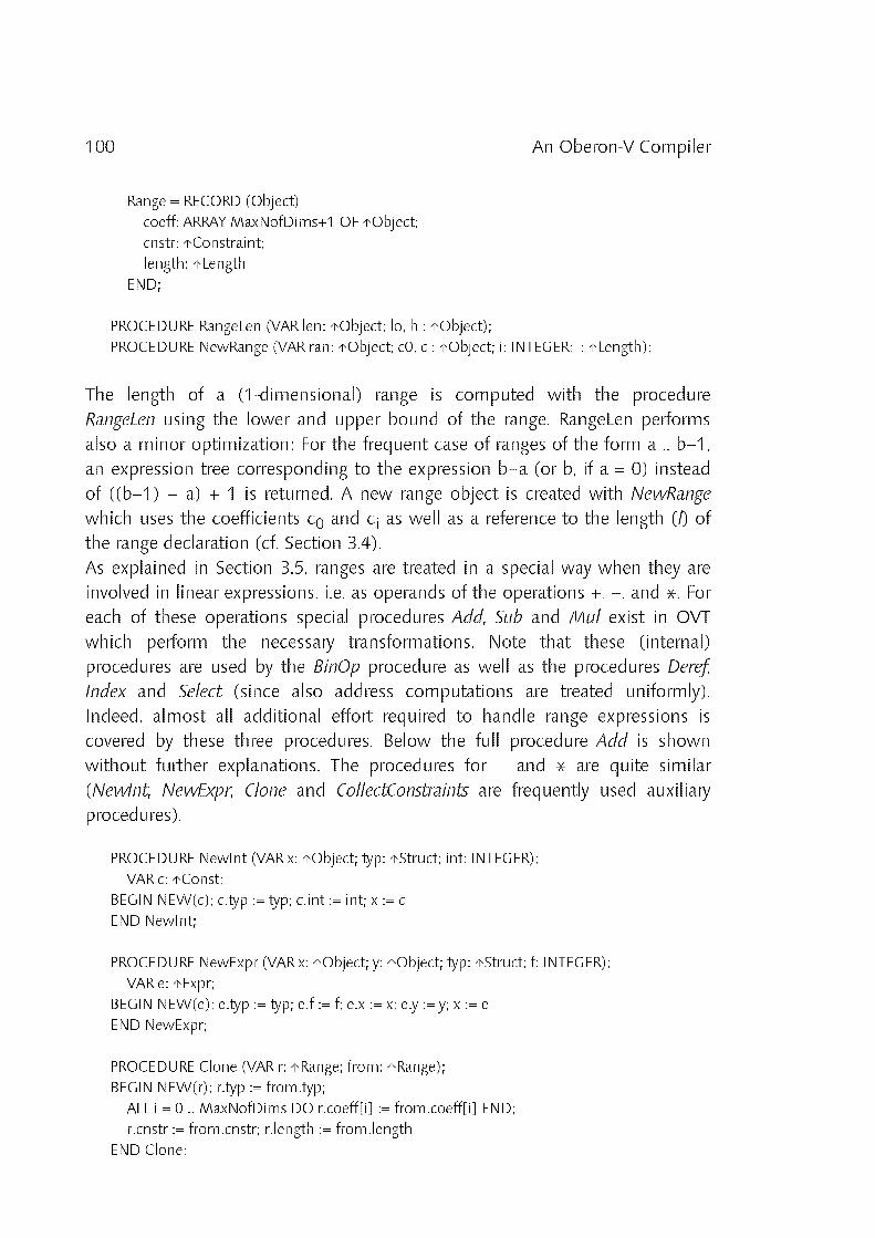
100 An Oberon_V Compiler
Range = RECORD (Object)
coeff: ARRAY MaxNofDims+1 OF ↑Object;
cnstr: ↑Constraint;
length: ↑Length
END;
PROCEDURE RangeLen (VAR len: ↑Object; lo, hi: ↑Object);
PROCEDURE NewRange (VAR ran: ↑Object; c0, ci: ↑Object; i: INTEGER; l: ↑Length);
The length of a (1_dimensional) range is computed with the procedureRangeLen using the lower and upper bound of the range. RangeLen performsalso a minor optimization: For the frequent case of ranges of the form a .. b−1,an expression tree corresponding to the expression b−a (or b, if a = 0) insteadof ((b−1) − a) + 1 is returned. A new range object is created with NewRange
which uses the coefficients c0 and ci as well as a reference to the length (l) ofthe range declaration (cf. Section 3.4).As explained in Section 3.5, ranges are treated in a special way when they areinvolved in linear expressions, i.e. as operands of the operations +, −, and *. Foreach of these operations special procedures Add, Sub and Mul exist in OVTwhich perform the necessary transformations. Note that these (internal)procedures are used by the BinOp procedure as well as the procedures Deref,Index and Select (since also address computations are treated uniformly).Indeed, almost all additional effort required to handle range expressions iscovered by these three procedures. Below the full procedure Add is shownwithout further explanations. The procedures for − and * are quite similar(NewInt, NewExpr, Clone and CollectConstraints are frequently used auxiliaryprocedures).
PROCEDURE NewInt (VAR x: ↑Object; typ: ↑Struct; int: INTEGER);
VAR c: ↑Const;
BEGIN NEW(c); c.typ := typ; c.int := int; x := c
END NewInt;
PROCEDURE NewExpr (VAR x: ↑Object; y: ↑Object; typ: ↑Struct; f: INTEGER);
VAR e: ↑Expr;
BEGIN NEW(e); e.typ := typ; e.f := f; e.x := x; e.y := y; x := e
END NewExpr;
PROCEDURE Clone (VAR r: ↑Range; from: ↑Range);
BEGIN NEW(r); r.typ := from.typ;
ALL i = 0 .. MaxNofDims DO r.coeff[i] := from.coeff[i] END;
r.cnstr := from.cnstr; r.length := from.length
END Clone;

101An Oberon_V Compiler
PROCEDURE CollectConstraints (VAR c: ↑Constraint; d: ↑Constraint);
VAR q: ↑Constraint;
BEGIN
WHILE d # NIL DO
NEW(q); q.next := c; c := q;
q.range := d.range; q.length := d.length;
d := d.next
END
END CollectConstraints;
PROCEDURE Add (VAR x: ↑Object; y: ↑Object);
VAR h: ↑Object; r, ry: ↑Range; i: INTEGER;
BEGIN
ASSERT((x.typ = y.typ) & ((x.typ = intTyp) | (x.typ = adrTyp)));
IF x IS Const THEN h := x; x := y; y := h END;
IF x IS Const THEN NewInt(x, x.typ, x{Const}.int + y{Const}.int)
ELSIF ˜(y IS Const) | (y{Const}.int # 0) THEN
IF x IS Range THEN h := x; x := y; y := h END;
IF x IS Range THEN
Clone(r, x{Range}); ry := y{Range}; i := ry.length.nofDims;
WHILE i >= 0 DO Add(r.coeff[i], ry.coeff[i]); DEC(i) END;
CollectConstraints(r.cnstr, ry.cnstr); x := r
ELSIF y IS Range THEN Clone(r, y{Range}); Add(x, r.coeff[0])
ELSE NewExpr(x, y, x.typ, add)
END
END
END Add;
Last but not least, two additional extensions of Objects are required in OVT:FuncCall and Address objects. While the former are used to represent functioncalls within expression trees (cf. Section 5.2.3), the latter represent machinespecific addresses and hence provide an interface to the compiler back_end.Address objects usually are extended in a back_end by machine specificattributes (e.g. register numbers or memory addresses). They are created by aback_end procedure to be installed in the global variable NewAddress.
TYPE
FuncCall = RECORD (Object)
proc: ↑Object;
args: ↑Assignment
END;
Address = RECORD (Object)
level: INTEGER;
leaf: BOOLEAN
END

102 An Oberon_V Compiler
VAR
NewAddress: PROCEDURE (level: INTEGER): Address;
The scope level of an address is stored in its level field; the level zero indicatesan address of a global variable (or procedure). If an address is used within anaddress computation or if it is referred to from within a nested scope, the leaf
field of the address object is set to FALSE. This information may be used by aback_end to decide whether a variable might be held in a register or whether itmust be held in memory.
5.2.2 Representation of Types
Each object is associated with a Struct node which describes the structure ofthe object's type. Like objects, different structures are best represented by typeextensions of the base type Struct. If a type has a name, the correspondingStruct node contains a reference to the associated identifier (id). The size of atype is the number of storage units required for variables of this type. This valueis inherently machine specific and hence is computed by means of theprocedure SetSize installed by the back_end. Arrays and records are structuredtypes and thus represented by extensions of the type Structured. This additionalextension level allows for convenient tests in the compiler (e.g. "IF typ ISStructured THEN ...") and for more expressiveness (e.g. a pointer's base typemust always be structured). Structured types also may have a type descriptor'saddress (desc) associated with them which is used to implement type guardsand type tests (cf. [Cohen 1991]).
TYPE
Struct = RECORD (Struct)
size: ↑Const;
id: ↑Object
END;
Structured = RECORD (Struct)
desc: ↑Address
END;
Array = RECORD (Structured)
length: ↑Const; (* length = NIL <=> open array *)
elemTyp: ↑Struct
END;

103An Oberon_V Compiler
Record = RECORD (Structured)
baseTyp: ↑Record;
scope: ↑Scope
END;
Pointer = RECORD (Struct)
pointeeTyp: ↑Structured
END;
Procedure = RECORD (Struct)
scope: ↑Scope;
resTyp: ↑Struct (* resTyp # NIL <=> function *)
END;
VAR
SetSize: PROCEDURE (typ: ↑Struct);
Arrays are determined by their length and the element type. Records aredescribed by their base type and their record fields, which are collected withinthe record scope. If a record type R1 is an extension of a record R, the prev fieldof the scope record associated with R1 points to the scope record associatedwith R (Figure 5.3). Thus, also record fields can be retrieved using the This
function mentioned in the beginning.
Example:
TYPE
R = RECORD
x: INTEGER
END;
R1 = RECORD (R)
a, b: REAL
END;
Scope
Scope Ident x
Scopenext
Ident R Ident R1
nextIdent a Ident b
Field Field
prev
prev
Field
Type Type
Record
Record
scope
scope
baseTyp
realTypintTyp
typ typ
typ
typ typ
Const 0
Const 0
Const 1
top scope
first
first
first
Figure 5.3 Representation of Records

104 An Oberon_V Compiler
All information used for a pointer type is its base type (pointeeTyp). Proceduretypes are determined by the procedure's parameter list and their result type, ifany. The procedure parameters as well as local variables are held in the samescope, the parameters beeing distinguished from local variables by the type ofthe representing object (Par instead of Var). Furthermore, parameters, if any, arealways at the beginning of an identifier list. The types of procedure objects(Proc) and the structure belonging to procedure types are represented in thesame way, namely by Struct nodes associated with a scope containing theprocedure parameters (Figure 5.4).
Example:
TYPE
P1 = PROCEDURE (x: REAL): REAL;
PROCEDURE P2 (x: REAL): REAL;
VAR a: INTEGER;
BEGIN
...
END P2;
Scope Ident ascope next
Ident xProced.
Par Var
Scopescope
Ident xProced.
Par
Scopenext
Ident P1 Ident P2
Type Proc
realTyp
resTyp
resTyp
prev
top scope
first
first
first
Figure 5.4 Representation of Procedures and Procedure Types
Finally, the module OVT provides a set of initialized global Struct variableswhich provide references to the Oberon_V basic types (cf. Appendix A.6.1) and afew internally used types (such as e.g. nilTyp or stringTyp):
VAR
undefTyp, adrTyp, nilTyp, stringTyp,
boolTyp, charTyp, setTyp, intTyp, realTyp, cmplxTyp: ↑Struct;
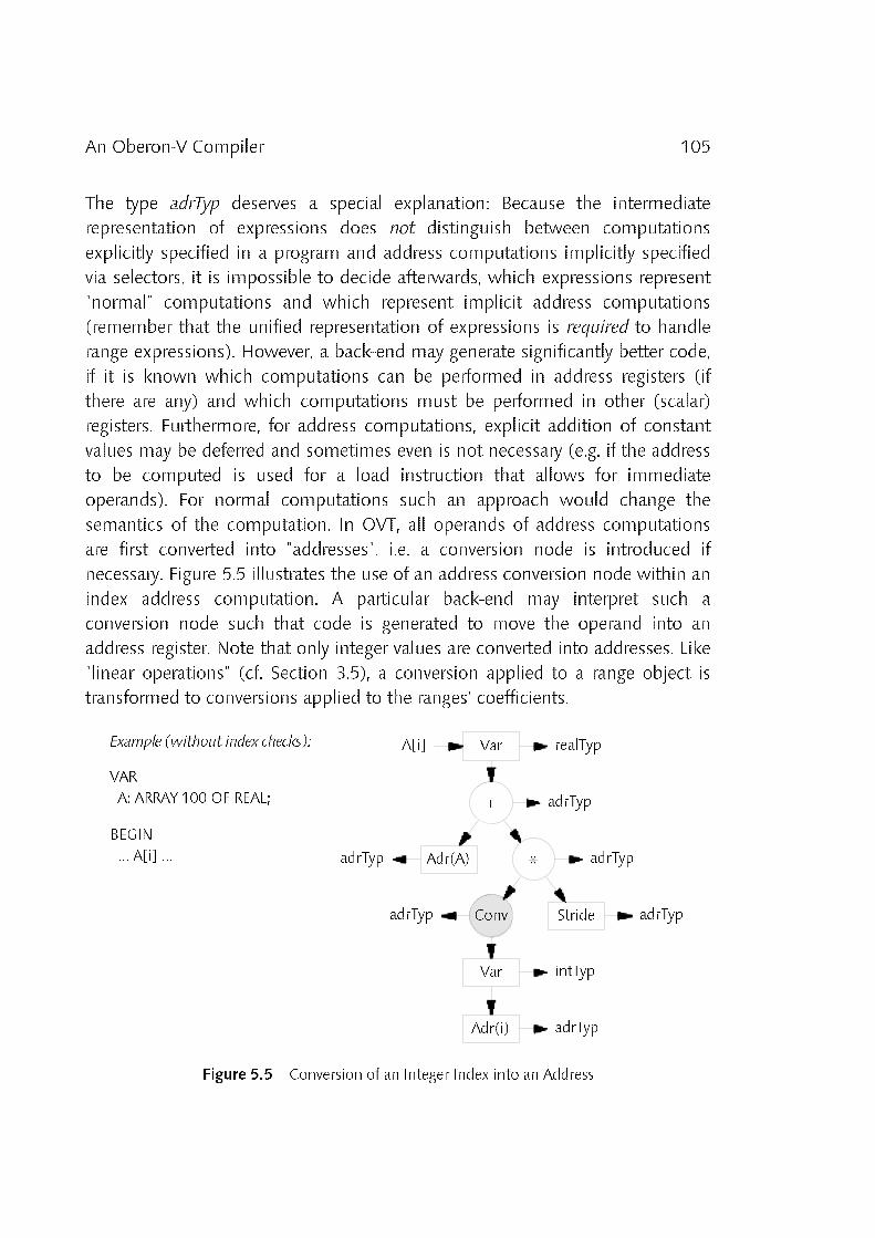
105An Oberon_V Compiler
The type adrTyp deserves a special explanation: Because the intermediaterepresentation of expressions does not distinguish between computationsexplicitly specified in a program and address computations implicitly specifiedvia selectors, it is impossible to decide afterwards, which expressions represent"normal" computations and which represent implicit address computations(remember that the unified representation of expressions is required to handlerange expressions). However, a back_end may generate significantly better code,if it is known which computations can be performed in address registers (ifthere are any) and which computations must be performed in other (scalar)registers. Furthermore, for address computations, explicit addition of constantvalues may be deferred and sometimes even is not necessary (e.g. if the addressto be computed is used for a load instruction that allows for immediateoperands). For normal computations such an approach would change thesemantics of the computation. In OVT, all operands of address computationsare first converted into "addresses", i.e. a conversion node is introduced ifnecessary. Figure 5.5 illustrates the use of an address conversion node within anindex address computation. A particular back_end may interpret such aconversion node such that code is generated to move the operand into anaddress register. Note that only integer values are converted into addresses. Like"linear operations" (cf. Section 3.5), a conversion applied to a range object istransformed to conversions applied to the ranges' coefficients.
Var
Var
+
*
Conv
A[i]
Stride
Adr(i)
Adr(A)
intTyp
adrTyp
adrTyp
adrTyp
adrTyp
adrTyp
adrTyp
realTypExample (without index checks):
VAR
A: ARRAY 100 OF REAL;
BEGIN
... A[i] ...
Figure 5.5 Conversion of an Integer Index into an Address

106 An Oberon_V Compiler
5.2.3 Representation of Statements
Procedures and modules may have bodies containing statement sequences.Statement sequences are represented as lists of extended Stat records (Figure5.6). For each statement, an appropriate record extension is used.
S1 S2 S3
next nextTYPE
Stat = RECORD
next: ↑Stat
END;
S1; S2; S3Stat Stat Stat
Figure 5.6 Representation of Statement Sequences
Assignments are represented by two expression trees, one for the left_hand sidedesignator and one for the right_hand side expression of the assignment (Figure5.7). An new assignment statement is generated using the procedure Assign
which checks whether the assignment is legal and which introduces additionalconversion nodes if necessary (e.g. to convert the result of an integer expressionto a real value). The same procedure is also used to generate parameter lists forprocedure calls (with param = TRUE, see below):
Assign.
dst src
TYPE
Assignment = RECORD (Stat)
dst, src: ↑Object
END;
PROCEDURE Assign (VAR stat: ↑Stat; dst, src: ↑Object; param: BOOLEAN);
Example:
d := e
Obj. d Obj. e
Figure 5.7 Representation of Assignments
Procedure calls are represented by ProcCall nodes, which contain a reference tothe called procedure object (which may be a procedure variable, too) as well asa list of assignments. Each assignment corresponds to a pair (parameter,argument). Figure 5.8 illustrates the data structure corresponding to a call of aprocedure P. The parameter objects are found in the scope of the calledprocedure.
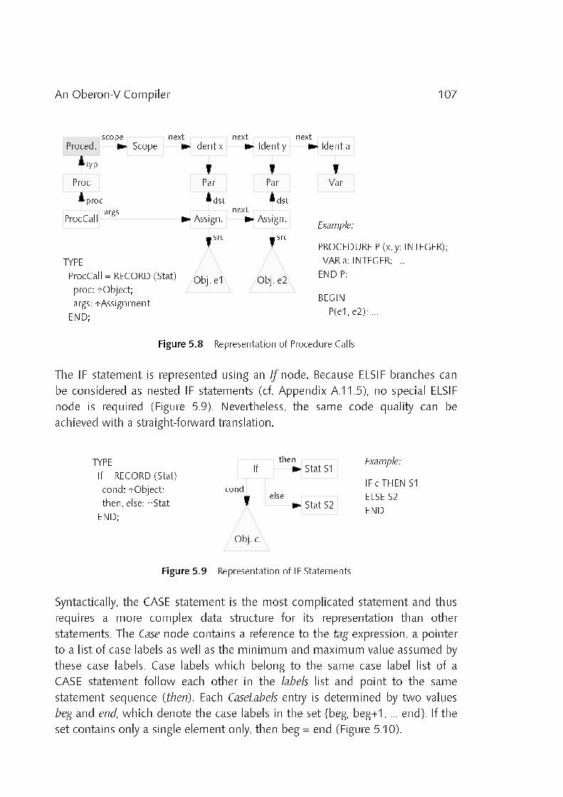
107An Oberon_V Compiler
nextScope
scope nextIdent xProced.
Par
Ident anext
VarPar
Ident y
Assign. Assign.args
Proc
ProcCall
proc
typ
next
src src
dst dst
TYPE
ProcCall = RECORD (Stat)
proc: ↑Object;
args: ↑Assignment
END;
Example:
PROCEDURE P (x, y: INTEGER);
VAR a: INTEGER; ...
END P;
BEGIN
P(e1, e2); ...
Obj. e1 Obj. e2
Figure 5.8 Representation of Procedure Calls
The IF statement is represented using an If node. Because ELSIF branches canbe considered as nested IF statements (cf. Appendix A.11.5), no special ELSIFnode is required (Figure 5.9). Nevertheless, the same code quality can beachieved with a straight_forward translation.
IfTYPE
If = RECORD (Stat)
cond: ↑Object;
then, else: ↑Stat
END;
cond
then
else
Stat S1
Stat S2
Obj. c
Example:
IF c THEN S1
ELSE S2
END
Figure 5.9 Representation of IF Statements
Syntactically, the CASE statement is the most complicated statement and thusrequires a more complex data structure for its representation than otherstatements. The Case node contains a reference to the tag expression, a pointerto a list of case labels as well as the minimum and maximum value assumed bythese case labels. Case labels which belong to the same case label list of aCASE statement follow each other in the labels list and point to the samestatement sequence (then). Each CaseLabels entry is determined by two valuesbeg and end, which denote the case labels in the set {beg, beg+1, ... end}. If theset contains only a single element only, then beg = end (Figure 5.10).
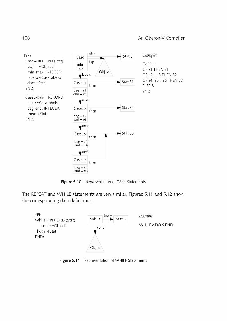
108 An Oberon_V Compiler
TYPE
Case = RECORD (Stat)
tag: ↑Object;
min, max: INTEGER;
labels: ↑CaseLabels;
else: ↑Stat
END;
CaseLabels = RECORD
next: ↑CaseLabels;
beg, end: INTEGER;
then: ↑Stat
END;
Example:
CASE e
OF e1 THEN S1
OF e2 .. e3 THEN S2
OF e4, e5 .. e6 THEN S3
ELSE S
END
Stat S1
Stat S2
Stat S3
beg = e1end = e1
beg = e2end = e3
beg = e4end = e4
beg = e5end = e6
Stat S
Obj. e
minmax
Case
CaseLb.
CaseLb.
CaseLb.
CaseLb.
next
next
next
labels
tag
else
then
then
then
then
Figure 5.10 Representation of CASE Statements
The REPEAT and WHILE statements are very similar; Figures 5.11 and 5.12 showthe corresponding data definitions.
While Stat S
Obj. c
Example:
WHILE c DO S ENDcond
bodyTYPE
While = RECORD (Stat)
cond: ↑Object;
body: ↑Stat
END;
Figure 5.11 Representation of WHILE Statements

109An Oberon_V Compiler
Stat S
Obj. c
Example:
REPEAT S UNTIL ccond
bodyTYPE
Repeat = RECORD (Stat)
cond: ↑Object;
body: ↑Stat
END;
Repeat
Figure 5.12 Representation of REPEAT Statements
The Return record type contains a reference to the returned object (val), if any. Aspecial Stat extension called BuiltIn is used to represent calls of predefinedprocedures such as NEW or HALT; such procedures are identified by aprocedure number (f) and they may have at most three arguments x, y, and z.BuiltIn statement nodes are created using the StdProcCall procedure, which alsoperforms the necessary checks.
TYPE
Return = RECORD (Stat)
val: ↑Object (* val = NIL <=> no return expression *)
END;
BuiltIn = RECORD (Stat)
f: INTEGER;
x, y, z: ↑Object
END;
PROCEDURE StdProcCall
(VAR stat: ↑Stat; proc: ↑StdProc; VAR args: ARRAY OF ↑Object; nofArgs: INTEGER);
Finally, a representation for ALL statements is required. As explained in Chapter3 (Section 3.7), an n_dimensional ALL statement is transformed into n nestedloops with corresponding prolog and epilog assignment sequences. Each loopneeds a counter variable and an initial value for this counter, namely the length
of the range declaration in this dimension. If the length of the innermost loop isshort, i.e. if the length of the n_th loop is constant and less than VLmax, noinnermost loop is required at all. This is signaled by a missing counter variablefor this loop (i.e. by counter[nofDims] = NIL). Furthermore, a list of constraints(cnstr) to be checked before executing the ALL statement is provided (cf.Section 3.9, Index Checks). The body field in the All record points to thestatement sequence corresponding to the transformed assignment sequenceenclosed by the ALL statement.

110 An Oberon_V Compiler
TYPE
All = RECORD (Stat)
prolog, epilog: ARRAY MaxNofDims+1 OF ↑Stat;
length: ARRAY MaxNofDims+1 OF ↑Object;
counter: ARRAY MaxNofDims+1 OF ↑Var;
nofDims: INTEGER;
cnstr: ↑Constraint;
body: ↑Stat
END;
PROCEDURE AllStat
(VAR stat: ↑Stat; lengths: ARRAY OF ↑Object; nofDims: INTEGER; scope: ↑Scope);
After compilation of the range declaration and the assignment sequence of ann_dimensional ALL statement, the assignment sequence (stat), the length of therange declaration, the number of dimensions (nofDims) as well as the currentscope are passed as arguments to AllStat. AllStat transforms the assignmentsequence as described in Section 3.7.2 and creates the necessary prolog andepilog statements. Auxiliary variables introduced during the transformation aswell as counter variables are simply appended in the current scope, usingidentifier names which cannot be used in a legal Oberon_V program. Thus, theyare invisible to the programmer but can be handled like other variables by thecompiler.
5.2.4 Representation of Entire Programs
Eventually one may have a look at the representation of entire programs. InOberon_V a compilation unit is a module. Modules are represented by Module
objects:
Type
Module = RECORD (Proc)
fingerprint: INTEGER
END;
From an operational view point, modules can be regarded as specialprocedures, and therefore they are represented by extensions of Proc objects (itis also convenient to do so, since code generation for modules and forprocedures is very much the same. Thus, this extension relation allows for asimilar treatment of procedures and modules in the back_end). The fingerprint
field is used for interface checks and is computed of the symbol file (seeSection 5.2.5). As with procedure objects, a module scope and a statement

111An Oberon_V Compiler
sequence are associated with a module object. The module scope contains alldeclarations, i.e. all globally declared identifiers which are used to refer to any(globally visible) object in the module. Note that also imported modules arecontained within this scope. Since local scopes and statement sequences ofprocedures are associated with the corresponding procedure objects, whichagain are referred to by its identifiers, a module identifier associated with amodule object may represent an entire program. This fact is also reflected bythe interface of the parser OVP (mid is the module identifier corresponding tothe compiled module):
MODULE OVP (OVT);
PROCEDURE Module (VAR mid: ↑OVT.Ident);
END OVP.
5.2.5 Import and Export
In an Oberon_V module, globally declared objects can be made available toother modules by means of exporting the corresponding identifiers. Vice versa,exported objects of other modules can be used by means of importing thecorresponding identifiers of these modules (cf. Appendix A, Sections A.4 andA.12). The collection of all exported objects constitutes a module's interface.Similar import/export mechanisms can be found in Modula_2 [Wirth 1885]and Oberon [Wirth 1988a].
In order to implement import and export safely, a compiler must know theinterfaces of imported modules. Usually this information is contained inso_called symbol files, which are generated as by_products of modulecompilations and which are read during the compilation of import lists.Roughly speaking, a symbol file contains a linearized description of a subset ofthe symbol table, namely the subset of all exported identifiers together withtheir associated object and type information. Thus, generating a symbol filemeans linearizing the symbol table, and reading a symbol file meansreconstructing parts of the symbol table from its linearized description.Although basic algorithms for the linearization of graphs and theirreconstruction are not difficult, their application to symbol files is significantlymore subtle, mostly because a single type can be imported several times throughdifferent modules. Thus, it is necessary to recognize whether two typesimported from different modules actually denote the same type or not. As afurther requirement, it is necessary that already compiled modules can easilydetect whether their imported modules have changed their interfaces. A simplesolution for this problem is to compute a (statistically) unique fingerprint, e.g.

112 An Oberon_V Compiler
an integer, from a symbol file and to use this fingerprint as an identification forthe whole interface. If the interface changes, also the fingerprint changes.
A new method for import and export based on a linearization algorithm forgeneral graphs has been developped. Since the problem is not directly relatedto the topic of this thesis, its implementation is not described here, but theinterested reader is referred to [Griesemer 1991]. The main advantage of thisalgorithm when compared with a solution currently used in Oberon compilers[Gutknecht 1985] is that recursive type definitions do not impose any problemsat all, whereas Gutknecht's solution requires a special treatment for recursivetype definitions via pointers (and would also for other forms of recursive typedefinitions, if they were allowed in current Oberon compilers). An elaboratetreatment of the import/export topic will be found in [Crelier 1993]. Also amechanism to extend a module interface afterwards without changing itsfingerprint will be described there.
5.3 Code Generation
After a compilation unit has been successfully parsed and the intermediate datastructure has been built, this data structure is passed to the back_end. Theback_end consists of four modules: The high_level code generator OVC, themodule OVE generating code patterns for expressions, the module OVV whichmanages the virtual code generated by OVE, and the low_level module OVO
which assembles the final Cray object file. In the following a rough survey ofthe modules OVC, OVE and OVV is given.
5.3.1 OVC: High Level Code Generation
The module OVC provides three services for code generation, namely theprocedures SetSize, AllocSpace and GenCode and thus corresponds to a similarmodule called OPV of the Oberon_2 compiler OP2 [Crelier 1990]:
MODULE OVC (OVT);
PROCEDURE SetSize (typ: ↑OVT.Struct);
PROCEDURE AllocSpace (pid: ↑OVT.Ident; VAR GSize: INTEGER);
PROCEDURE GenCode (pid: ↑OVT.Ident);
END OVC.
113An Oberon_V Compiler
SetSize computes the size required for variables of arbitrary type (typ); theprocedure is installed in the global variable OVT.SetSize (cf. Section 5.2.2) bythe command module OV. Before starting code generation via GenCode, theprocedure AllocSpace is called which computes the addresses of variables (andparameters) local to a procedure or module specified by their identifiers (pid).For each scope, all identifiers are sorted according to the value of their usage
field (cf. Section 5.2.1). Variables referred to by identifiers with high usage areprocessed first and hence register locations may be allocated for them, if theiraddresses are leaf. The address information for variables as well as additionaldata (such as the total size of all local variables, etc.) are held in extensions ofAddress objects associated with Var and Par (or Proc) objects; the extension isdefined in module OVE. The global data size (GSize) is also computed byAllocSpace. Note that no distinction is required between variables in localscopes and variables in module scopes, but address allocation is determinedonly by the exported and usage information of Ident nodes as well as the level
and leaf fields of Address objects (cf. Section 5.2.1). Thus, global variables thatare used only in the initialization statement sequence of a module may also beallocated in registers or on the run_time stack. Finally, GenCode is used totraverse the scope of a procedure or module (pid). GenCode is called recursivelyfor each local procedure. After traversing a procedure's scope, GenCodegenerates code for the syntax tree corresponding to the procedure's statementsequence.
Code generation can be regarded as a transformation of the syntax tree intoa linearized sequence of machine instructions. A systematic and efficientapproach is to map every node of the syntax tree into a semantically equivalentcode sequence, which then is appended to the code already generated. In theOberon_V compiler, a simple technique is used which proved to be successfulin a series of similar compilers [Wirth 1985a][Wirth 1992][Brandis et. al. 1992].In order to generate code for a node S, first, code is generated for all itsdescendant nodes S1, S2, ... Sn. Information about the code generated for anode Sk is returned in an attribute xk. The attributes x1, x2, ... xn are then usedto generate the code for S. The attribute x describing the code for S may in turnbe used by the parent of S, and so on. Thus, if the (well_understood) influenceof the symbol table is ignored, a context_free translation of nodes Sk isobtained. For a given node S, its code Code(S) is a function FS of the Code(Sk)generated for its descendant nodes Sk:
Code(S) = FS(Code(S1), Code(S2), ... Code(Sn))
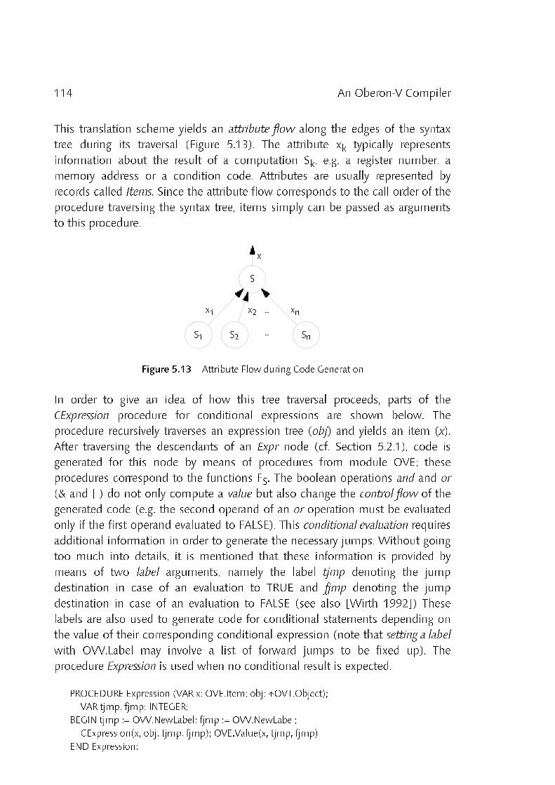
114 An Oberon_V Compiler
This translation scheme yields an attribute flow along the edges of the syntaxtree during its traversal (Figure 5.13). The attribute xk typically representsinformation about the result of a computation Sk, e.g. a register number, amemory address or a condition code. Attributes are usually represented byrecords called Items. Since the attribute flow corresponds to the call order of theprocedure traversing the syntax tree, items simply can be passed as argumentsto this procedure.
S
S S S1 2 n
x x x1 2 n
...
...
x
Figure 5.13 Attribute Flow during Code Generation
In order to give an idea of how this tree traversal proceeds, parts of theCExpression procedure for conditional expressions are shown below. Theprocedure recursively traverses an expression tree (obj) and yields an item (x).After traversing the descendants of an Expr node (cf. Section 5.2.1), code isgenerated for this node by means of procedures from module OVE; theseprocedures correspond to the functions FS. The boolean operations and and or
(& and | ) do not only compute a value but also change the control flow of thegenerated code (e.g. the second operand of an or operation must be evaluatedonly if the first operand evaluated to FALSE). This conditional evaluation requiresadditional information in order to generate the necessary jumps. Without goingtoo much into details, it is mentioned that these information is provided bymeans of two label arguments, namely the label tjmp denoting the jumpdestination in case of an evaluation to TRUE and fjmp denoting the jumpdestination in case of an evaluation to FALSE (see also [Wirth 1992]) Theselabels are also used to generate code for conditional statements depending onthe value of their corresponding conditional expression (note that setting a labelwith OVV.Label may involve a list of forward jumps to be fixed up). Theprocedure Expression is used when no conditional result is expected.
PROCEDURE Expression (VAR x: OVE.Item; obj: ↑OVT.Object);
VAR tjmp, fjmp: INTEGER;
BEGIN tjmp := OVV.NewLabel; fjmp := OVV.NewLabel;
CExpression(x, obj, tjmp, fjmp); OVE.Value(x, tjmp, fjmp)
END Expression;
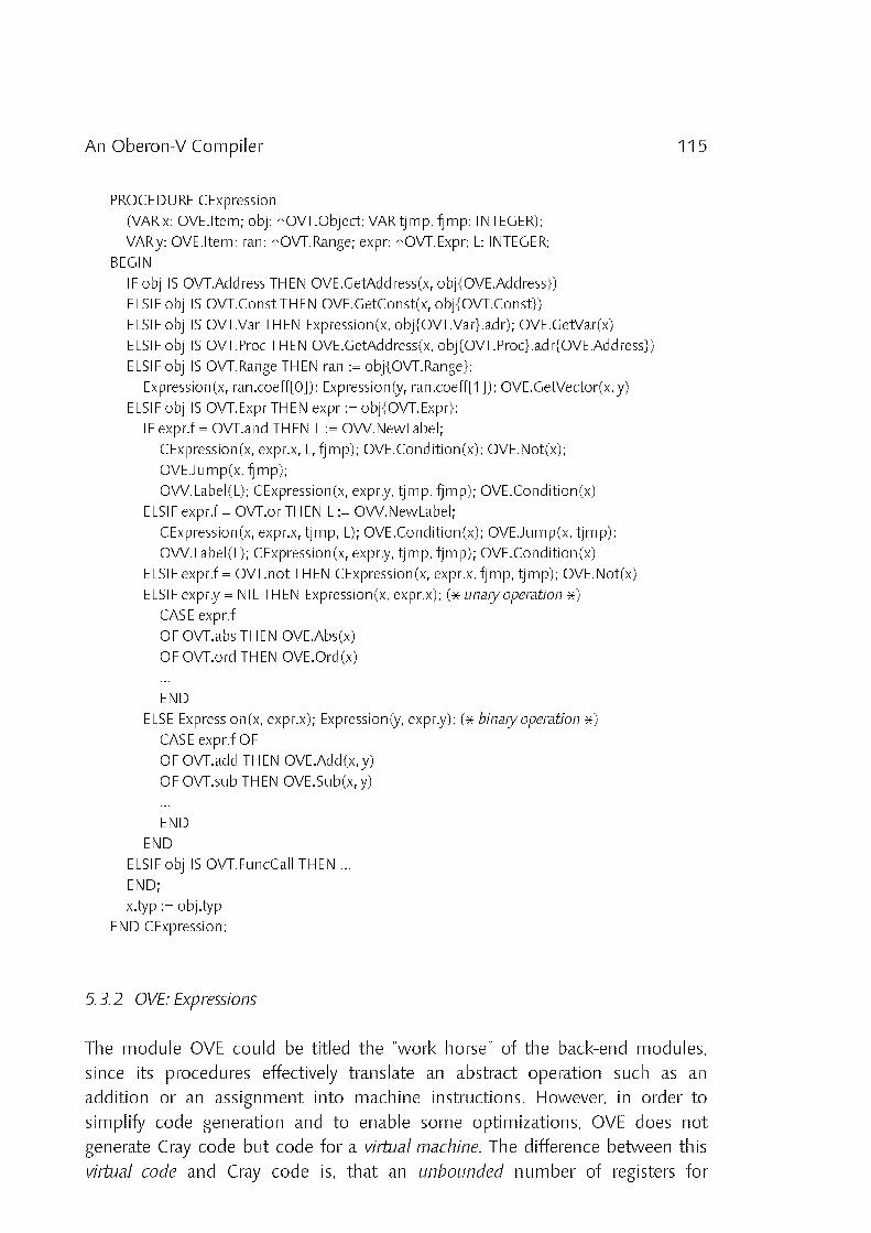
115An Oberon_V Compiler
PROCEDURE CExpression
(VAR x: OVE.Item; obj: ↑OVT.Object; VAR tjmp, fjmp: INTEGER);
VAR y: OVE.Item; ran: ↑OVT.Range; expr: ↑OVT.Expr; L: INTEGER;
BEGIN
IF obj IS OVT.Address THEN OVE.GetAddress(x, obj{OVE.Address})
ELSIF obj IS OVT.Const THEN OVE.GetConst(x, obj{OVT.Const})
ELSIF obj IS OVT.Var THEN Expression(x, obj{OVT.Var}.adr); OVE.GetVar(x)
ELSIF obj IS OVT.Proc THEN OVE.GetAddress(x, obj{OVT.Proc}.adr{OVE.Address})
ELSIF obj IS OVT.Range THEN ran := obj{OVT.Range};
Expression(x, ran.coeff[0]); Expression(y, ran.coeff[1]); OVE.GetVector(x, y)
ELSIF obj IS OVT.Expr THEN expr := obj{OVT.Expr};
IF expr.f = OVT.and THEN L := OVV.NewLabel;
CExpression(x, expr.x, L, fjmp); OVE.Condition(x); OVE.Not(x);
OVE.Jump(x, fjmp);
OVV.Label(L); CExpression(x, expr.y, tjmp, fjmp); OVE.Condition(x)
ELSIF expr.f = OVT.or THEN L := OVV.NewLabel;
CExpression(x, expr.x, tjmp, L); OVE.Condition(x); OVE.Jump(x, tjmp);
OVV.Label(L); CExpression(x, expr.y, tjmp, fjmp); OVE.Condition(x)
ELSIF expr.f = OVT.not THEN CExpression(x, expr.x, fjmp, tjmp); OVE.Not(x)
ELSIF expr.y = NIL THEN Expression(x, expr.x); (* unary operation *)
CASE expr.f
OF OVT.abs THEN OVE.Abs(x)
OF OVT.ord THEN OVE.Ord(x)
...
END
ELSE Expression(x, expr.x); Expression(y, expr.y); (* binary operation *)
CASE expr.f OF
OF OVT.add THEN OVE.Add(x, y)
OF OVT.sub THEN OVE.Sub(x, y)
...
END
END
ELSIF obj IS OVT.FuncCall THEN ...
END;
x.typ := obj.typ
END CExpression;
5.3.2 OVE: Expressions
The module OVE could be titled the "work horse" of the back_end modules,since its procedures effectively translate an abstract operation such as anaddition or an assignment into machine instructions. However, in order tosimplify code generation and to enable some optimizations, OVE does notgenerate Cray code but code for a virtual machine. The difference between thisvirtual code and Cray code is, that an unbounded number of registers for

116 An Oberon_V Compiler
expression evaluation is assumed. The instructions themselves are (nearly) thesame. As will be explained in the next section, this allows for some powerfuloptimizations. Furthermore, it relieves module OVE from handling registerallocation for temporary values (i.e. for expression results, etc.).
To provide the prerequisites for understanding the OVE data structures, abrief description of the Cray architecture is given. A Cray Y_MP processor offers5 different register files, namely 8 scalar address registers (A_registers) of 32 bitswidth, 8 scalar general_purpose registers (S_registers) of 64 bits width and 8vector registers (V_registers). Each vector register may hold at most 64 elementsof 64 bits width each, i.e. VLmax = 64. Additionally, there are two register fileswith 64 temporary registers each, called B_ and T_registers. B_registers have awidth of 32 bits, T_registers may hold 64_bit values. These temporary registersare used to hold local variables and to pass procedure arguments. Addresscomputations are performed using the A_registers; conventional scalararithmetics is done using the S_registers and vector instructions operate on theV_registers. The instruction set is very similar to the instruction set of thehypothetical machine introduced in Section 1.1. Note that for almost alloperations op three instruction variants exist:
Si := Sj op SkSi := Sj op VkSi := Vj op Vk
For a general description of the Cray architecture and its instruction set, thereader is referred to [Russel 1978], [Robbins 1987] and [Cray 1988]. In thefollowing, only a rough survey of the internals of the module OVE is given. Theonly data types exported are the type Address, an extension of OVT.Address, aswell as the Item data type (where only the typ field is exported):
Address = RECORD (OVT.Address)
mode, reg, adr, rel: INTEGER;
LSize, ... : INTEGER
END
Item = RECORD
typ: ↑OVT.Struct;
mode, reg, ireg, adr, rel, n: INTEGER
END
The mode, reg, adr and rel fields of an Address object specify the location of avariable or procedure: the mode field determines, which of the remaining fieldsis valid; reg corresponds to a register number; adr and rel specify a memory

117An Oberon_V Compiler
address and possible relocation information required to generate Cray objectfiles. The fields LSize, etc. are used for procedures (and modules) only andspecify the stack requirements and the number of local variables held inregisters.
The architecture of a code generator and thus also the module OVE isstrongly influenced by the addressing modes provided by the target machine.These addressing modes find their direct representation in the different modes
of items. An Item record specifies (the location of) a value. Figure 5.14 showsthe possible contents of item records and their interpretation. Note that usingtype extension to represent different item modes would be unpractical becauseitems frequently change their modes during their life times, and every modechange would require to allocate a new item.
VCond x cond vector mask
VectorI x stride M[(Areg) + i*(Aireg)]
Vector x stride (A/Sreg) + i*(A/Sireg)
VregI x x M[(Areg) + (Vireg[i])]
VregO x x x x (Areg) + (Vireg[i]) + adrrel
Vreg x (x) (Vreg[i])
Cond x cond condition
Sreg x (x) (Sreg)
AregI x x x M[(Areg) + adrrel]
AregO x x x (Areg) + adrrel
Areg x (Areg)
Treg x (Tn)
Breg x (Bn)
Const value constant
Proc * level label x adrrel
Mem * level x x (FPlevel) + adrrel
TregN * x Tn
BregN * x Bn
mode reg ireg n adr rel meaning
Figure 5.14 Item Modes and Interpretation
Modes which are marked (*) appear also as modes for address objects. A_, S_and V_register numbers (fields reg and ireg) specify virtual registers; they startwith the number 8. Register numbers smaller than 8 are interpreted asimmediate operands. Especially, the register number 0 denotes the value 0 (or0.0, depending on the item type) and the register number 1 the value 1 (or 1.0

118 An Oberon_V Compiler
respectively). This encoding is useful to improve code generation for operationson complex numbers and also to denote special vector strides (e.g. vectors withstride 1; they can be loaded with a special instruction).
Constant values (mode = Const) are always held in an item record itself(field n). A value held in a register is represented by an item with mode Areg,Sreg, Vreg, Breg or Treg; the register number is specified by the reg field. In caseof a complex number, i.e. where the item type is cmplxTyp, the ireg fieldspecifies the S_ or V_ register holding the imaginary part of the number or vector(which may also be a constant, namely 0.0 or 1.0, using the encoding schemeexplained before). Real and imaginary parts held in T_registers or in mainmemory are always stored consequtively, thus a single address suffices in thesecases. Variables held in memory are represented by items with modes AregI,Mem, VregI and VectorI. The relocation field rel is valid only if it contains apositive value.
The BregN, TregN, AregO, VregO and Vector modes deserve a specialexplanation: Since no distinction is made between conventional and addresscomputations by the front_end, and because addresses (which may be simpleregister numbers) appear also in expression trees, they consequently appear alsoas items. Here, these modes simply denote a B_ or T_register number, a (scalar)memory address, a vector of memory addresses or a vector address respectively.During traversal of an expression tree, each occurrence of a Var node implies acorresponding transition of the corresponding item mode from a modedenoting an address to a mode denoting a variable at this address. Theprocedure GetVar performs this transition:
PROCEDURE GetVar (VAR x: Item);
VAR v: INTEGER;
BEGIN
CASE x.mode OF
OF BregN THEN x.mode := Breg
OF TregN THEN x.mode := Treg
OF Breg, Treg, Areg, AregI, Sreg THEN LoadA(x); x.mode := AregI; x.adr := 0; x.rel := −1
OF AregO THEN x.mode := AregI
OF Vreg, VregI, VectorI THEN LoadV(x); x.mode := VregI; x.ireg := x.reg; x.reg := 0
OF VregO THEN v := x.ireg; x.mode := AregO; ToAreg(x); x.mode := VregI; x.ireg := v
OF Vector THEN x.mode := VectorI
END
END GetVar;
Figure 5.15 illustrates the OVE procedure calls, the transition of the item modesand the code generated for a simple addition of two variables. The (small)numbers 1, 2, ... 5 indicate the visiting order of each node.

119An Oberon_V Compiler
Var Var
Adr(a) Adr(b)
+
GetAddress(x, ...)x.mode = TregN
x.reg = 6
GetVar(x)x.mode = Treg
x.reg = 6
GetAddress(y, ...)y.mode = TregN
y.reg = 7
GetVar(y)y.mode = Treg
y.reg = 7
Add(x, y)x.mode = Sreg
x.reg = 24
a + b
1
2 4
3
5
Code generated at step 5:
S22 := T6
S23 := T7
S24 := S22 + S23
Figure 5.15 Transition of Item Modes for Scalar Addition
For each operation of the language Oberon_V, a procedure is provided bymodule OVE. Each of these procedures usually accepts one or two itemarguments x and y describing the (location of the) operands. After execution ofa particular procedure, the item x describes the computed value (the value of yis undefined).
PROCEDURE GetAddress (VAR x: Item; adr: ↑Address);
PROCEDURE GetConst (VAR x: Item; con: ↑OVT.Const);
PROCEDURE GetVar (VAR x: Item);
PROCEDURE GetVector (VAR x, stride: Item);
...
PROCEDURE Abs (VAR x: Item);
PROCEDURE Ord (VAR x: Item);
...
PROCEDURE Add (VAR x, y: Item);
PROCEDURE Sub (VAR x, y: Item);
...
Procedure GetVector constructs a vector item with mode = Vector from itsaddress (x, stride). The items for x and stride are directly obtained by evaluatingthe c0 and c1 coefficients of the corresponding range object (cf. previoussection, procedure CExpression). Note that at this stage of code generation, onlyrange objects with two coefficients occur. If an OVE procedure is called withvector items as arguments, the corresponding vector instructions are generatedinstead of scalar code. Fig. 5.16 shows the OVE procedure calls, the transition ofitem modes and the generated code for the addition of a vector and a scalarvalue.

120 An Oberon_V Compiler
+
Var
cc
Var
Var
Adr(c)
Const 1
Adr(v)GetAddress(x)x.mode = BregN
x.reg = 14
GetVar(x)x.mode = Breg
x.reg = 14
GetConst(x, ...)y.mode = Const
y.n = 1
GetAddress(y)y.mode = TregN
y.reg = 4
GetVar(y)y.mode = Treg
y.reg = 4
Add(x, y)x.mode = Vreg
x.reg = 46
GetVector(x, y)x.mode = Vector
x.reg = 43
x.ireg = 1
GetVar(x)x.mode = VectorI
x.reg = 43
x.ireg = 1
1
2 3
4
5
6
7
8
Code generated at step 4:
A43 := B14Code generated at step 8:
V44 := M[1, A43]
S45 := T4
V46 := S45 + V44
ALL r = 0 .. 63 DO
... v[r] + c ...
END
0 1
Figure 5.16 Transition of Item Modes for Vector Addition
Note the special interpretation of the constant stride in step 4: Since vectorswith stride 1 can be loaded with special vector load instructions which requireonly a single register argument (the start address), no A_register for the stride isintroduced. Instead, it is represented by the special register number 1 whichdenotes the immediate value 1.
5.3.3 OVV: The Virtual Machine Code
The module OVV contains data structures and procedures to store andoptimize virtual machine code. In the sequel two optimizations applied to thisvirtual code are described briefly. For clarity the instructions of the hypotheticalmachine introduced in Section 1.1 are used. The basic difference whencompared with the virtual instructions used for the Cray Y_MP is the restrictionto 2 register files (the S_ and V_registers) instead of 5 register files. Since theoptimizations described here can be applied both to scalar and vectorinstructions, it is concentrated on scalar instructions only.
Common Subexpression Elimination, or CSE for short, is the elimination ofredundant computations, i.e. the elimination of instructions which calculate anexpression that has been calculated before. CSE can be done on different levels

121An Oberon_V Compiler
during the compilation process but is most effective when applied to a programrepresentation which closely mirrors the available machine instructions. This isdue to the fact that translation itself may introduce new commonsubexpressions which were not apparent when CSE would be applied earlier(e.g. address computations for array elements). The CSE algorithm used inmodule OVV is based on a well_known technique called value numbering
[Cocke 1970]. As an example, let us consider the code generation for theexpression A[i+1, j] + A[i+1, k] where A is a 100 x 100 real array and i, j and kdenote integer variables. The algorithm works as follows: For every virtualinstruction computing a new value, a new destination register is allocated(which also explains the name value numbering). This preserves all previouslycomputed values and hence they can be accessed in any subsequentcomputation. For the first term A[i+1, j] the following code is generated:
; S0 address of A
; S1 variable i
; S2 variable j
; S3 variable k
;
S10 := 1 + S1 ; i+1
S11 := 100 * S10 ; (i+1)*100
S12 := S2 + S11 ; (i+1)*100 + j
S12 := M[S0 + S12] ; A[i+1, j]
Before generating a new instruction, the already generated instructions aresearched for an equivalent instruction. If such an instruction is found, no codeis emitted but the destination register of the already existing instruction is usedinstead. The following example illustrates the code generation for A[i+1, k]:
; S13 := 1 + S1 1+S1 has been computed already: use S10
; S13 := 100 * S10 100 * S10 has been computed already: use S11
;
S13 := S3 + S11 ; (i+1)*100 + k
S14 := M[S0 + S13] ; A[i+1, k]
S15 := S12 +F S14 ; A[i+1, j] + A[i+1, k]
In the example the expression i+1 must be computed to determine the arrayoffset for the second term. Scanning backwards in the instruction streamreveals that the same computation has been performed already, and that theresult is in register S10 (and must still be there because of the consecutiveregister numbering). Instead of generating an add instruction and introducing anew register, the value in register S10 is used. The same happens, when anattempt is made to compute (i+1) * 100. The value i+1 is in S10, thus a

122 An Oberon_V Compiler
multiply instruction 100*S10 should be generated. Scanning backwards revealsthat the result of 100 * S10 is held already in S11; thus no code must beemitted but S11 can be used instead. When continuing this way, all redundantinstructions will be eliminated and optimal code (as far as CSE is concerned)results.
Further improvement is achieved, by a special treatment of commutativeoperations: Obviously, an instruction S10 * S11 yields the same result as S11 *S10. It is a good idea to normalize instructions for commutative operations, e.g.such that the first register operand always has the smaller register number.Often, such a normalization is required anyway in order to have an immediateoperand at the right position in the instruction format.
In OVV, the virtual code is simply stored in an array. Each array elementcorresponds to a virtual instruction. The element index can be regarded asprogram counter and also corresponds to the destination register number, whichtherefore has not to be stored explicitly. Note that the CSE algorithm as it hasbeen presented here must be applied within extended basic blocks only, i.e. nolabel must occur within the code stretch to be optimized, except at its verybeginning. Furthermore, special precautions are required for load and storeinstructions; these topics are not discussed here. CSE would be relatively slowwithout optimizations: Before the i_th instruction can be generated, all i−1previous instructions in the basic block must be inspected and compared withthe new instruction in question. For a sequence of n redundancy freeinstructions, (n2−n)/2 comparisons are necessary in total; i.e. the algorithm hasa run_time complexity of O(n2). In OVV, all instructions denoting the sameoperation are chained in the instruction array. Thus, searching backwardsrequires only searching instructions denoting the same operation. In practice analmost linear run_time is achieved.
To give an idea of the implementation, the procedure Op2 and parts of therequired data structures are shown below. Op2 is responsible for binaryoperations op applied on two operands held in virtual registers j and k. Theresult of the computation is assigned to the virtual register i (corresponding tothe instruction index in the Code array). Op2 is used in module OVE whenever abinary operation has to be generated. The Root array contains the roots of allinstruction chains linking instructions with the same op field.
CONST
NofInstr = ... ; CodeSize = ... ;

123An Oberon_V Compiler
VAR
Root: ARRAY NofInstr OF INTEGER;
Code: ARRAY CodeSize OF RECORD
op, j, k, ... : INTEGER; (* instruction Sj op Sk *)
link: INTEGER; (* previous instruction with same op field; −1 denotes end of chain *)
...
END;
PROCEDURE Commutative (op: INTEGER): BOOLEAN; (* TRUE if op is commutative *)
PROCEDURE Insert (op: INTEGER; VAR i: INTEGER; j, k: INTEGER); (* inserts new instr. *)
PROCEDURE Op2 (op: INTEGER; VAR i: INTEGER; j, k: INTEGER);
BEGIN
IF (j > k) & Commutative(op) THEN i := j; j := k; k := i END; (* canonical form: j <= k *)
i := Root[op];
WHILE (i >= 0) & ((Code[i].j # j) OR (Code[i].k # k)) DO i := Code[i].link END;
IF i < 0 THEN (* no CSE found *) Insert(op, i, j, k) END
END Op2;
As a final example for CSE its application to extended basic blocks is shown:Since jumps do not invalidate the current contents of the virtual registers, theircontents may also be reused after a jump, i.e. across basic block boundaries.Thus, a statement sequence in a THEN branch may also profit from commonsubexpressions in the conditional expression of an IF statement. In the examplebelow, the code in the THEN branch is reduced to a single instruction only.Also redundant index checks are eliminated this way in OVV (not shown here).
IF A[i, j] < x THEN A[i, j] := x END
; S0 address of A
; S1 variable i
; S2 variable j
; S3 variable x
;
S10 := 100 * S1 ; i*100
S11 := S2 + S11 ; i*100 + j
S12 := M[S0 + S11] ; A[i, j]
S13 := S12 <F S3 ; A[i, j] < x
Jump End (˜S13) ; IF A[i, j] < x THEN
M[S0 + S11] := S13 ; A[i, j] := x
End ... ; END
The second optimization performed in OVV is Instruction Scheduling or IS forshort: In pipelined computers the execution of an instruction is divided intoseveral suboperations that are executed sequentially on several independent

124 An Oberon_V Compiler
units, called pipestages. With this organization, multiple instructions mayexecute concurrently and each instruction occupies a different pipestage (Figure5.17). At time t instruction a is in pipestage 1, at time t+1 instruction a is inpipestage 2 and b is in pipestage 1, etc.
t+1 t+2 t+3 t+4 t+5 t+6Time
t
1
2
3
Pipestage
a
a
a
b
b
b
c
c
c
d
d
delay
Instructions
Figure 5.17 Pipelined Execution of Instructions
An instruction depending on the result of a previous instruction must not beissued until the required result is available. That is, either the compiler ensuresthat the instruction is not issued too early or the processor delays theinstruction until its operands become available (pipeline interlock). In Figure5.17, instruction d is assumed to use an operand (a register) computed byinstruction b and thus cannot be issued at time t+3 but must wait untilinstruction b has terminated at t+4. Pipeline interlocks due to such timing
hazards may significantly decrease the performance of a program. On Craymachines (cf. [Robbins 1987]) and many popular RISC architectures (e.g. MIPS[Kane 1987] or SPARC [Sun 1987]) instructions are executed in a such apipelined fashion and hence a compiler should carefully avoid pipelineinterlocks imposed by the generated code. This is achieved by instruction
scheduling, i.e. the reordering of instructions such that interlocks are avoided butthe effect of the program is preserved. In the example it were possible to swapthe instructions a and b, assuming that a and b are independent. This wouldreduce the execution time of the four instructions a ... d by 1 clock cycle (Figure5.18).

125An Oberon_V Compiler
t+1 t+2 t+3 t+4 t+5 t+6Time
t
1
2
3
Pipestage
a
a
a
b
b
b
c
c
c
d
d
Figure 5.18 Pipelined Execution of Instructions after Scheduling
The IS problem is well_studied in the literature and approaches for its solutiongo back to methods originally developed for microcode compaction [Landskov1980]. A thorough survey of research can be found in [Gross 1983] or[Hennessy 1983]. Like many practical problems, IS is NP_complete (see e.g.[Gross 1983]) and hence only heuristic solutions are likely to be practicable.Register allocation may introduce additional dependences that can restrict thepossibilities for instruction reordering. On the other hand, IS may increaseregister pressure, i.e. the number of registers that are alive at a specific time, andhence complicates register allocation. Thus, register allocation and IS pursueconflicting goals. There are pre_ and postpass solutions: the former reorderinstructions before register allocation is done (e.g. [Auslander 1982], one of theapproaches described in [Gross 1993] or the solution used here), the latterperform IS after register allocation (e.g. [Gibbons 1986], [Davidson 1984] and[Davidson 1986]). Recent work tries to improve the situation by usinginformation of the scheduling phase to drive register allocation [Bradlee 1991].
The most common IS algorithms are variations of list scheduling ([Landskov1980], [Gibbons 1986], [Warren 1990]): A dependence graph is constructed foreach basic block. Nodes of the graph represent machine instructions and edgesdenote dependences; an edge from node a to node b indicates that a must beexecuted before b in order to preserve the overall effect of the basic block. Theset of all nodes that have no predecessor, i.e. the set of instructions that dependon no other instruction, is called the candidate set (Figure 5.19).

126 An Oberon_V Compiler
S10 := S0 + S1
S11 := 2 * S10
S12 := S4 − S3
S13 := 10 + S12
S14 := S11 * S13
S15 := S10 / S12
S16 := S5 * S11
S17 := S14 / S15
(S0 ... S5 are assumed to
be available already)
S10 := S0 + S1
S11 := 2 * S10
S12 := S4 − S3
S13 := 10 + S12
S14 := S11 * S13
S15 := S10 / S12
S16 := S5 * S11
S17 := S14 / S15
Candidate Set
Figure 5.19 Dependence Graph and Candidate Set for a Basic Block
The list scheduling algorithm corresponds to a topological sort of the graphnodes and proceeds as follows: While the candidate set and hence the graph isnot empty, a suitable instruction i of the candidate set is selected according tosome heuristics and its node is removed from the graph. Note that anyinstruction j that had instruction i as its single predecessor, has no predecessorafter removing i and then enters the candidate set. A simple framework for listscheduling can be formulated in Oberon_V:
PROCEDURE Schedule (G: Graph; Select: PROCEDURE (G: Graph): Node);
VAR n: Node;
BEGIN
WHILE ˜Empty(G) DO
n := Select(Candidates(G));
Remove(G, n);
Emit(n)
END
END Schedule;
The quality of a list scheduling algorithm depends on the selection heuristic.Although list scheduling has a worst_case run_time proportional to O(n2) wheren is the number of instructions, a linear behavior can be expected for practicalcases [Gibbons 1986].
List scheduling appears to be a relatively simple technique for instructionscheduling: basically, the dependence graph corresponds to the expression treedrawn upside down (see Figure 5.19). Nevertheless, a simpler method wasdeveloped for the Oberon_V compiler [Griesemer 1992]. The method profitsfrom the representation of virtual code by an array: For IS, instead of appending

127An Oberon_V Compiler
consecutive instructions, they are inserted in the code array at the earliestpossible location determined by data dependences and possible interlocks.Using the array representation mentioned for CSE, the program counter can betaken as the destination register number. Assuming that a new instruction isissued every clock cycle (without interlocks), the program counter may also beinterpreted as the current clock. This leads to a surprisingly simple method fordirectly placing an instruction while observing its dependences.
Let I(a, b) be an instruction depending on the contents of registers a and b(i.e. the results of the instructions a and b). When E(a) and E(b) are theexecution times of these instructions, a+E(a) and b+E(b) are the times wheneach result is available. Consequently, both results are available at Max(a+E(a),b+E(b)), which is the earliest possible location for I.
Let us assume an execution time of 2 cycles for addition and memory loadand 3 cycles for multiplication (there are much longer execution times for CrayY_MP instructions). In the array expression example, the computation 100 *S10 depends on S10 and the earliest issue time is 12 = Max(0, 10+2), since thetime used to compute S10 is 2 cycles and the operand 100 is availableimmediately. Instead of simply appending the instruction as before at position11, it is inserted at position 12. Note that the destination register number isautomatically determined by the instruction position and has not to be stored.The resulting free instruction slots at position 11 may be thought as being filledwith a no_op instruction. Continuing this way, the following instructionsequence for A[i+1, j] is obtained:
; S0 address of A
; S1 variable i
; S2 variable j
; S3 variable k
PC Execution time Result available
10 S10 := 1 + S1 ; i+1 2 12
11 no_op
12 S12 := 100 * S10 ; (i+1)*100 3 15
13 no_op
14 no_op
15 S15 := S2 + S12 ; (i+1)*100 + j 2 17
16 no_op
17 S17 := M[S0 + S15] ; A[i+1, j] 2 19
Hence, whenever a new instruction has to be inserted, its earliest issue time isdetermined due to its data dependences and the instruction is then inserted atthe calculated position. Inserting an instruction after the end of the currentcode block extends the block. When inserting an instruction in the middle of

128 An Oberon_V Compiler
the code block, the instruction replaces the next free instruction slot (possibly atthe end of the code block). Eventually, the following code for A[i+1, j] + A[i+1,k] is obtained:
; S0 address of A
; S1 variable i
; S2 variable j
; S3 variable k
PC Execution time Result available
10 S10 := 1 + S1 ; i+1 2 12
11 no_op
12 S12 := 100 * S10 ; (i+1)*100 3 15
13 no_op
14 no_op
15 S15 := S2 + S12 ; (i+1)*100 + j 2 17
16 S16 := S3 + S12 ; (i+1)*100 + k 2 18
17 S17 := M[S0 + S15] ; A[i+1, j] 2 19
18 S18 := M[S0 + S16] ; A[i+1, k] 2 20
19 no_op
20 S20 := S17 +F S18 ; A[i+1, j] + A[i+1, k]
The rules are a little bit more complex if store instructions are involved: Topreserve the effect of a code sequence, the relative ordering of consecutiveloads and stores must remain unchanged. These problems are not discussedhere.
After generating the virtual code for an extended basic block, it must betranslated into the target machine code. That is, for each virtual instruction one(or several) target machine instructions have to be selected and final registerallocation must be done. When register pressure is too high, spill code has to beinserted. In OVV this translation is done by an additional sweep over the virtualcode. A brief overview on this translation process is given in the sequel:
Target instruction selection: Since the virtual instructions differ from the targetmachine instructions only in the unbounded number of registers used, this partof the translation process is trivial: When the final register numbers are known,the final machine instructions can be generated directly.
Register allocation: At this level only registers for temporaries occurring duringexpression evaluation have to be allocated. In the OV compiler, the A_, S_ andV_registers are used for this purpose. During translation of the virtual code intofinal machine code, whenever a new result is computed, an appropriatephysical register is allocated from these register files using a simple round_robinalgorithm. The physical register number is remembered together with thecorresponding virtual register. Whenever the virtual register is referenced again,the physical register number is used instead. At some point, the virtual register
129An Oberon_V Compiler
is not referenced any more and the corresponding physical register should bereleased. To detect this situation, a simple technique which has been describedin [Freiburghouse 1974] is used. The key idea is to assign a reference counter toevery virtual register, i.e. instruction in the array representation. Duringgeneration of the virtual code, this reference counter is increased whenever thecorresponding register is referenced by another instruction. During target codegeneration, whenever a virtual register is referenced, the corresponding referencecounter is decreased. When it drops to zero, this was the last reference to thevirtual register and hence the corresponding physical register can be released.
Spill code generation: When straight_forward code is generated forexpressions (without CSE or IS), very few registers are usually required to holdtemporaries. However, CSE and IS significantly raise register pressure. Evenwhen reserving eight or more registers for expression evaluation, excessiveregister demand may require to spill currently unused registers to memory.When spilling to memory, reload instructions have to be inserted which mayimpose new interlocks.
In case of the Cray Y_MP, spilling is relatively cheap because a good portionof the temporary B_ and T_register files is reserved for this purpose. Load andstore accesses to temporary registers are executed in one cycle, therefore noadditional interlocks are introduced. Spilling to main memory would beimpractical due to the long latency of load instructions. Note that only local
spilling is necessary, i.e. within basic blocks. This is in contrast to simpleChaitin_like graph_coloring techniques for register allocation which globally (i.e.for an entire procedure) decide, which values have to reside in memory [Chaitin1982]. Nevertheless, the decision which register to spill is difficult and dependshighly on the context in which the register is used. As a simple heuristic, inOVV the physical register which has not been used for the longest time isspilled.
5.4 Hardware Support
Some problems related to code generation for the particular instruction set ofthe Cray Y_MP have not been discussed yet. In fact, this instruction set hassome deficiencies which make the generation of correct code cumbersome. It isinteresting that most of these deficiencies apply also to an older architecture,namely the CDC 6000 series (already pointed out in [Wirth 1972]). Thisrelationship may not surprise since Seymour Cray worked also on the design ofthe CDC 6600 and CDC 6700 machines. For the sake of brevity the details arenot discussed but the main trouble spots are summarized only:

130 An Oberon_V Compiler
1. No overflow check on integer arithmetic. For both, the 32 bit and 64 bitregisters, there is no hardware support to detect integer overflows. The price forguarding all integer operations is prohibitive.
2. No compare instructions. Conditional jumps depend on the comparison ofthe A0_ or S0_registers with zero. A general comparison of the form x rel y istransformed to (x−y) rel 0. If overflow occurs in the subtraction (which is notsimply detectable), the result of the relational expression is wrong.
4. No arithmetic shift instructions. Since also no instruction for sign extensionis available, an arithmetic shift right instruction must be emulated by a lengthysequence of logical and arithmetic operations.
5. No support for 64_bit integer multiplication/division. 64_bit integermultiplication and division is performed using floating point arithmetics. Sincefull 64_bit results would require subroutine calls or inlined code sequences ofup to 30 instructions for multiplication and even more instructions for division,currently only 46_bit multiplication and division are implemented in Oberon_V.
Besides these deficiencies, the Cray Y_MP is quite clean and orthogonal, thusmaking a clean and small code generator possible. Nevertheless, from theviewpoint of the compiler writer, we would like to propose a single major pointthat should be improved (increased), namely the number of general purpose
registers. Each of the three general_purpose register files (A_, S_ and V_registers)provides only 8 registers. Furthermore, the A0 and S0 registers can be read by afew instructions only, thus making them worthless for expression evaluation.When common subexpression elimination and instruction scheduling isperformed, register pressure is quite high and frequently spilling is required.Hence, it is difficult to allocate local variables in these register files. Currently,such variables are held in the two temporary register files (B_ and T_registers),thus requiring additional register_register moves if they are accessed. Largergeneral_purpose registers (and the omission of the temporary registers) wouldsimplify the code generator and probably also improve the execution speed ofthe generated code.

6 Measurements
Some empirical results on a small collection of typical subroutines andprograms are presented. All the measurements have been done on a Cray Y_MP[Cray 1988]. If not specified otherwise, the results are given in clock cycles, thecycle time is 6ns. Although only average values are presented here, the resultsmay not be very accurate: since the Cray Y_MP is a multi_processorshared_memory system, a running process may be delayed because of memorybank conflicts caused by other processors. The estimated relative error is5−10%.
6.1 BLA Subprograms
The Basic Linear Algebra Subprograms or BLAS for short [Lawson 1979] have beenvery successful and are used in a wide range of numerical software includingpackages such as Linpack (see Section 6.2). They have become a de factostandard for elementary vector operations. In the following a collection ofmeasurements made for four frequently used BLA procedures, namely sscal,saxpy, sasum and sdot is shown (cf. Appendix B.1). In Oberon_V theseprocedures reduce to simple "one_liners" which preferably are used directlyinstead of calling the subroutine.
Table 6.1 shows the measurements for these four BLA procedures, differentvector lengths (n) and different (combinations of) compiler options: /x meanswithout index checks, /i turns instruction scheduling (IS) off, /c disablescommon subexpression elimination (CSE) and /ic is without CSE and IS. Alltimes are given in clock cycles per element. The right_most column shows theresults obtained with the Cray Fortran compiler cft77. To obtain comparable
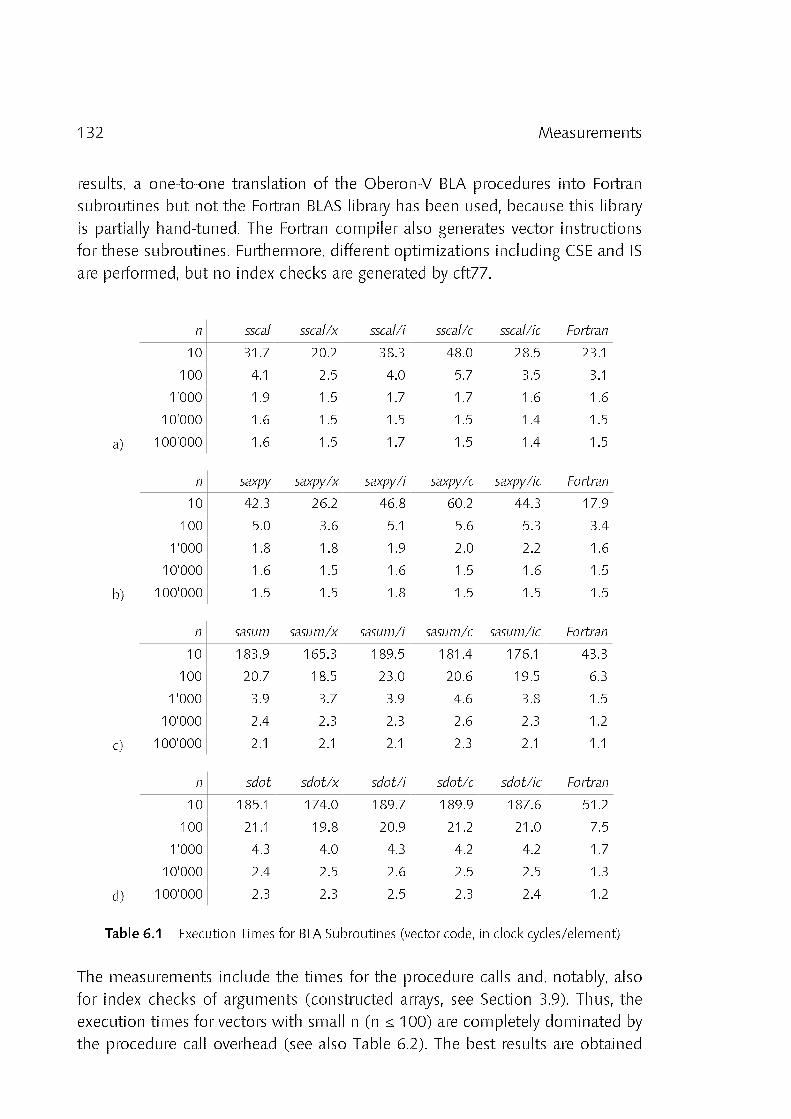
132 Measurements
results, a one_to_one translation of the Oberon_V BLA procedures into Fortransubroutines but not the Fortran BLAS library has been used, because this libraryis partially hand_tuned. The Fortran compiler also generates vector instructionsfor these subroutines. Furthermore, different optimizations including CSE and ISare performed, but no index checks are generated by cft77.
a) 100'000 1.6 1.5 1.7 1.5 1.4 1.5
10'000 1.6 1.5 1.5 1.5 1.4 1.5
1'000 1.9 1.5 1.7 1.7 1.6 1.6
100 4.1 2.5 4.0 5.7 3.5 3.1
10 31.7 20.2 38.3 48.0 28.5 23.1
n sscal sscal/x sscal/i sscal/c sscal/ic Fortran
b) 100'000 1.5 1.5 1.8 1.5 1.5 1.5
10'000 1.6 1.5 1.6 1.5 1.6 1.5
1'000 1.8 1.8 1.9 2.0 2.2 1.6
100 5.0 3.6 5.1 5.6 5.3 3.4
10 42.3 26.2 46.8 60.2 44.3 17.9
n saxpy saxpy/x saxpy/i saxpy/c saxpy/ic Fortran
c) 100'000 2.1 2.1 2.1 2.3 2.1 1.1
10'000 2.4 2.3 2.3 2.6 2.3 1.2
1'000 3.9 3.7 3.9 4.6 3.8 1.5
100 20.7 18.5 23.0 20.6 19.5 6.3
10 183.9 165.3 189.5 181.4 176.1 43.3
n sasum sasum/x sasum/i sasum/c sasum/ic Fortran
d) 100'000 2.3 2.3 2.5 2.3 2.4 1.2
10'000 2.4 2.5 2.6 2.5 2.5 1.3
1'000 4.3 4.0 4.3 4.2 4.2 1.7
100 21.1 19.8 20.9 21.2 21.0 7.5
10 185.1 174.0 189.7 189.9 187.6 51.2
n sdot sdot/x sdot/i sdot/c sdot/ic Fortran
Table 6.1 Execution Times for BLA Subroutines (vector code, in clock cycles/element)
The measurements include the times for the procedure calls and, notably, alsofor index checks of arguments (constructed arrays, see Section 3.9). Thus, theexecution times for vectors with small n (n # 100) are completely dominated bythe procedure call overhead (see also Table 6.2). The best results are obtained

133Measurements
when index_checks are disabled. However, because index checks are performedonly once before executing the ALL statement, for larger n no significantdifference is noticed anymore. Also the effect of the optimizations disappearsfor large n, which is a clear indication that they influence mostly the (scalar)code for procedure calls, index checks and loop initialization. When comparedwith Fortran, for n 3 1000 the same or even better results are obtained for sscaland saxpy (Table 6.1 a) and b). In case of sasum and sdot (Table 6.1 c) and d)however, only half the execution speed of the corresponding Fortran code isachieved. It seems that this difference is mainly due to a better but also morecomplicated code pattern for reduction loops generated by the Fortran compiler(the Fortran code proceeds in steps of 128 instead of 64 vector elements anduses two vector registers for the partial sums; see also Section 3.8.2).
Table 6.2 shows the timings for the same BLA procedures, when no vectorinstructions are used (compiler option /v) but scalar code is generated for theALL statements and the SUM function. The numbers in the right_most column(loops) have been measured for conventionally implemented BLA proceduresusing WHILE loops instead of ALL statements.
a) 100'000 40.5 40.4 56.2 42.4 60.1 74.3
10'000 40.3 40.4 56.2 42.4 60.2 74.3
1'000 40.5 40.7 56.6 42.8 60.4 74.6
100 43.0 43.1 58.9 45.3 63.1 77.4
10 68.3 66.1 84.1 67.0 88.9 104.1
n sscal/v sscal/vx sscal/vi sscal/vc sscal/vic loops
b) 100'000 49.1 49.6 80.4 52.0 85.3 99.3
10'000 49.2 50.0 80.4 52.0 85.4 99.4
1'000 49.5 50.5 80.6 52.4 85.8 99.6
100 52.6 56.1 83.6 55.5 89.3 102.6
10 83.9 116.3 115.2 87.4 123.8 130.4
n saxpy/v saxpy/vx saxpy/vi saxpy/vc saxpy/vic loops
c) 100'000 41.4 41.3 49.4 41.9 51.3 73.6
10'000 41.5 41.4 49.2 41.3 51.3 73.7
1'000 41.7 41.5 49.6 41.3 51.5 73.9
100 43.3 43.0 51.3 43.2 53.9 77.2
10 59.6 57.8 67.3 75.4 76.1 116.1
n sasum/v sasum/vx sasum/vi sasum/vc sasum/vic loops
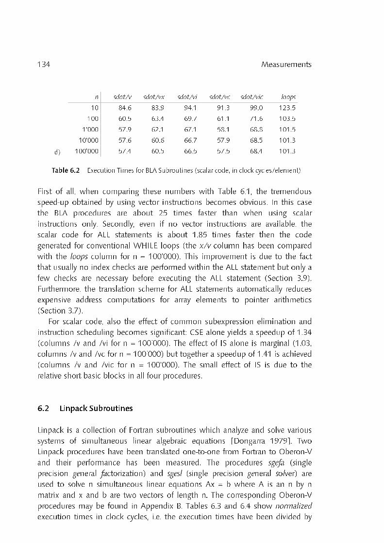
134 Measurements
d) 100'000 57.4 60.5 66.5 57.5 68.4 101.3
10'000 57.6 60.6 66.7 57.9 68.5 101.3
1'000 57.9 62.1 67.1 58.1 68.8 101.5
100 60.5 63.4 69.7 61.1 71.6 103.5
10 84.6 83.9 94.1 91.3 99.0 123.5
n sdot/v sdot/vx sdot/vi sdot/vc sdot/vic loops
Table 6.2 Execution Times for BLA Subroutines (scalar code, in clock cycles/element)
First of all, when comparing these numbers with Table 6.1, the tremendousspeed_up obtained by using vector instructions becomes obvious. In this casethe BLA procedures are about 25 times faster than when using scalarinstructions only. Secondly, even if no vector instructions are available, thescalar code for ALL statements is about 1.85 times faster then the codegenerated for conventional WHILE loops (the x/v column has been comparedwith the loops column for n = 100'000). This improvement is due to the factthat usually no index checks are performed within the ALL statement but only afew checks are necessary before executing the ALL statement (Section 3.9).Furthermore, the translation scheme for ALL statements automatically reducesexpensive address computations for array elements to pointer arithmetics(Section 3.7).
For scalar code, also the effect of common subexpression elimination andinstruction scheduling becomes significant: CSE alone yields a speedup of 1.34(columns /v and /vi for n = 100'000). The effect of IS alone is marginal (1.03,columns /v and /vc for n = 100'000) but together a speedup of 1.41 is achieved(columns /v and /vic for n = 100'000). The small effect of IS is due to therelative short basic blocks in all four procedures.
6.2 Linpack Subroutines
Linpack is a collection of Fortran subroutines which analyze and solve varioussystems of simultaneous linear algebraic equations [Dongarra 1979]. TwoLinpack procedures have been translated one_to_one from Fortran to Oberon_Vand their performance has been measured. The procedures sgefa (singleprecision general factorization) and sgesl (single precision general solver) areused to solve n simultaneous linear equations Ax = b where A is an n by nmatrix and x and b are two vectors of length n. The corresponding Oberon_Vprocedures may be found in Appendix B. Tables 6.3 and 6.4 show normalized
execution times in clock cycles, i.e. the execution times have been divided by

135Measurements
the following values:
for sgefa: n3/3for sgesl: n2
These values roughly estimate the number of "axpy_operations" executed bysgefa and sgesl, i.e. the number of assignment statements of the form y[i] :=a*x[i] + y[i]. For example, a value 1.8 indicates that 1.8 clock cycles have beenused on average for an axpy_operation.
1000 2.0 1.8 2.5 2.2
900 2.0 1.8 2.7 2.2
800 2.1 1.9 2.8 2.2
700 2.2 2.0 2.9 2.3
600 2.3 2.0 3.2 2.3
500 2.4 2.1 3.5 2.3
400 2.7 2.3 4.0 2.4
300 3.1 2.6 4.9 2.5
200 3.8 3.2 6.5 2.7
100 6.3 5.0 11.8 3.7
n sgefa sgefa/x sgefa/ic Fortran
Table 6.3 Execution Times of sgefa (in clock cycles/axpy_op)
If index checks are omitted (sgefa/x) an average speedup of 1.15 is achieved.Again, for larger n the effect of index checks becomes smaller. On the otherhand, the effect of CSE and IS is quite high: both optimizations yield an averagespeedup of almost 1.47 (for all n, columns sgefa and sgefa/ic). When comparedwith Fortran, the Oberon_V code (sgefa/x) is slower for small n (n < 300) butthe same or even better performance is achieved for larger n. In general, muchbetter scalar code is generated by the Fortran compiler. This also explains theleading position of Fortran for small n; an observation made before (Section6.1). However, a detailed investigation of these effects is beyond the scope ofthis thesis.

136 Measurements
1000 1.9 1.8 2.4 1.4
900 2.0 1.8 2.5 1.4
800 2.1 1.9 2.6 1.4
700 2.2 1.9 2.7 1.5
600 2.2 2.0 2.9 1.5
500 2.4 2.1 3.2 1.6
400 2.7 2.3 3.6 1.7
300 3.1 2.5 4.3 1.9
200 3.8 3.1 5.8 2.3
100 6.2 4.8 10.2 3.5
n sgesl sgesl/x sgesl/ic Fortran
Table 6.4 Execution Times of sgesl (in clock cycles/axpy_op)
In Table 6.4 essentially the same results as in Table 6.3 can be observed. Theimprovement obtained by omitting index checks decreases for large n and thespeedup gained by CSE and IS is 1.35 on average. For n = 1000, every 2 clockcycles an axpy operation containing two floating_point operations is performedby sgefa. For a cycle time of 6ns this corresponds to a performance of167MFlops. Together with sgefa, a system of 1000 simultaneous linearequations can be solved in approximately 4s.
In Fortran arrays are mapped to memory in column_major order, i.e.consecutive elements of a matrix column are mapped to consecutive memorywords. Thus, if an algorithm processes a matrix column_wise, usually the vectorstride is one. In Oberon_V arrays are mapped in row_major order and hence thestride of a column vector is usually greater than one. Accessing such vectorsmay lead to memory bank conflicts and hence to significant delays (for anintroduction into interleaved memory systems see for example [Hennessy1990]). Indeed, the Linpack subroutines essentially rely on the array mapping of
Fortran and they perform badly for certain values of n if they are translated toOberon_V in a one_to_one way. However, instead of rewriting all algorithmssuch that they process rows instead of columns, the same effect can beobtained easily in Oberon_V by transposing the matrix using an arrayconstructor:
PROCEDURE Work (VAR a: ARRAY OF ARRAY OF REAL, ...);
(* do anything with a *)
ENDWork;
BEGIN ...
Work([i, j = 0 .. LEN(a)−1: a[j, i]], ...); ...

137Measurements
If a certain array mapping is required within a procedure (e.g. column_majororder instead of row_major_order), the appropriate array is simply passed as aparameter. When the procedure is called, the desired mapping (e.g. atransposition) is performed using an array constructor. Note that this does notmean that the array is copied, but only that the array mapping is changed whichdoes not impose any additional run_time costs. Using this technique, variouskinds of memory mappings can be tested without changing an algorithm.
6.3 Compiler Data
Finally, a survey of the size and the compilation speed of the Oberon_Vcompiler OV is given. Table 6.5 illustrates the sizes of individual modules in(non_empty) lines of code (Lines) and in the number of statements (Stats). Thesize of the object code for the Ceres_2 workstation [Heeb 1988] containing aNS32532 CPU is given in KB. The right_most column shows the object codesizes of corresponding modules of the Oberon_2 compiler NOP2 for the samemachine [Mössenböck 1991][Crelier 1990]. Apparently, when ignoring moduleOVV, both compilers have the same size. In contrast, the size of the CrayFortran compiler cft77 is 4.7MB which is more than 50 times the size of theOberon_V compiler.
Total 5970 6010 90.2 74.5
OV User Interface 80 80 1.3 2.0 (NOP2)
OVC Tree Traversal 620 620 10.1 6.6 (NOPV)
OVE Expressions 1400 1400 18.7 17.4 (NOPC)
OVV Virtual Code 700 790 16.2 − −
OVO Object Files 430 470 7.7 8.8 (NOPL)
OVP Parser 770 850 9.3 11.4 (NOPP)
OVT Table Handler 1670 1470 23.6 24.9 (NOPT + NOPB)
OVS Scanner 300 330 3.3 3.4 (NOPS)
Module Functionality Lines Stats Code NOP2
Table 6.5 Size of the Oberon_V compiler OV (in KB)
In order to determine the compilation speed of the Oberon_V compiler,procedures of a longer module (containing a collection of Linpack procedures)have been removed step_by_step and the time for its compilation with respectto different compiler options has been measured (Table 6.6). Overall, thecompilation time is nearly linear in the program length for all options (the
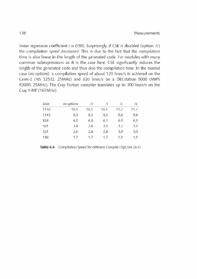
138 Measurements
linear regression coefficient r is 0.98). Surprisingly, if CSE is disabled (option /c)the compilation speed decreases! This is due to the fact that the compilationtime is also linear in the length of the generated code. For modules with manycommon subexpressions as it is the case here, CSE significantly reduces thelength of the generated code and thus also the compilation time. In the normalcase (no options), a compilation speed of about 120 lines/s is achieved on theCeres_2 (NS 32532, 25MHz) and 620 lines/s on a DECstation 5000 (MIPSR3000, 25MHz). The Cray Fortran compiler translates up to 300 lines/s on theCray Y_MP (167MHz).
186 1.7 1.7 1.7 1.9 1.9
321 2.6 2.6 2.6 3.0 3.0
501 3.8 3.8 3.9 4.3 4.4
828 6.0 6.0 6.1 6.9 6.9
1143 8.3 8.3 8.3 9.4 9.4
1146 10.1 10.1 10.1 11.7 11.7
Lines no options /v /i /c /ic
Table 6.6 Compilation Speed for different Compiler Options (in s)

7 Summary and Conclusions
Section 7.1 gives a brief survey of our achievements, whereas Section 7.2 pointsout some features that could be improved. Finally, conclusions are draw inSection 7.3
7.1 What has been achieved
We have introduced two language constructs, namely the ALL statement and anew form of array constructors, both oriented towards the programming ofnumerical applications for vector computers. The constructs have beenintegrated into a new programming language called Oberon_V, a descendant ofthe programming language Oberon [Wirth 1988a]. A possible implementationscheme has been described and an experimental Oberon_V compiler for theCray Y_MP vector computer has been constructed. We have implemented a fewtypical applications in Oberon_V and have compared their performance withcorresponding Fortran solutions.
The ALL statement allows to express directly independence of a sequence ofassignment statements and thus can always be translated into vectorinstructions, as long as no conditional expressions occur. Unfortunately, acompiler cannot check in general whether assignments enclosed in an ALLstatement are independent or not. Thus, it is the programmer's responsibility toprove its correct usage. In our experience, for practical cases the requiredindependence property is rather easy to show or even obvious. For difficultcases however a compiler will not be able to solve the problem instead. Wemay compare this situation with the use of a conventional loop where (in thegeneral case) also the programmer alone can ensure its termination.

140 Summary and Conclusions
The provability of programs cannot be measured objectively. However, thecorrectness of programs using ALL statements is easier to prove than thecorrectness of programs using corresponding loops, because overspecificationssuch as the execution order or additional statements for incrementinginduction variables can be avoided. Furthermore, since a programmer mayexplicitly state that parts of a program can be executed in parallel, a reader ofthe program is also directly informed about this fact and thus may gain adeeper insight into an algorithm.
The translation of ALL statements requires neither complicated analysistechniques nor time_consuming optimizations but is obtained by a simpletransformation of its internal representation and a second traversal of this datastructure for final code generation. For typical applications the execution speedof the generated code is comparable with the execution speed of the codegenerated by the Cray Fortran compiler. We have implemented additionaloptimizations on the instruction level, such as common subexpressionelimination and a simple instruction scheduling algorithm for scalarinstructions. Though the effect of these optimizations tends to be completelyovershadowed by the effect of vector instructions as long as only ALLstatements are considered. However, we must not conclude that suchoptimizations are worthless: if only one half of the executed code of a programcan be vectorized due to Amdahl's Law, a speedup of a factor two may beachieved in the best case, but only if the vectorized program portion wouldexecute in zero time. A reasonable scalar performance is therefore required toobtain good results.
Array constructors are a powerful and clean construct to specify arbitrarysubarrays as procedure arguments. Similar mechanisms exist in otherlanguages, but they usually do not offer the same flexibility or are inacceptablyinefficient for the aim pursued here (e.g. the call_by_name mechanism of Algol60 [Naur 1960]). The implementation of array constructors goes hand_in_handwith the implementation of ALL statements. Indeed, almost the entirecompiling machinery introduced for ALL statements has been reused toimplement array constructors. Since array constructors can only be used asarguments for open array parameters, they only impose additional costs if theextra flexibility is really needed.
The Oberon_V cross_compiler has been implemented in Oberon and runsunder the Oberon System [Wirth 1988b]. It consists of some 6000 lines ofcode or about 90KB object code for the Ceres_2 workstation [Heeb 1988]. Thecompilation speed is about 120 lines/s on the Ceres_2 (NS 32532, 25MHz) and620 lines/s on a DECstation 5000 (MIPS R3000, 25MHz). These figurescompare favorably with the Fortran_77 compiler on the Cray with about 4.7MB

141Summary and Conclusions
object code size and a compilation speed of 300 lines/s (Cray Y_MP, 167MHz).
7.2 What could be improved
1. An ALL statement describes a set of assignment sequences that must beindependent of each other, i.e. two different assignment sequences must notmodify the same variable. Thus, if in a particular sequence a temporary value iscomputed which is to be used later in the same sequence, an array with thesame dimensionality as the ALL statement must be introduced. If it werepossible to declare some kind of "local variables" within ALL statements, suchan array would be unnecessary. The following example illustrates a possiblesolution:
ALL r = a .. b WITH t: REAL DO
t := a[r] * b[r];
b[r] := t * c1;
c[r] := t + c2
END
The identifier t is visible within the scope of the ALL statement only. Fordifferent values of the range identifier r, different variables are denoted by t. Asimilar approach has been chosen in the FORALL statement in Vienna Fortran[Zima et. al. 1992], a Fortran extension oriented towards multiprocessorarchitectures with distributed memory.
2. We have described the translation of an ALL statement into a sequence ofvector or scalar instructions for a single_processor machine. It should not be toocomplicated to generate code for a multiprocessor machine (e.g. the Cray Y_MPcan be equipped with up to eight processors). The key idea is simple: for amachine with n processors, the index set specified by the range declaration ofan ALL statement is divided into n subsets, e.g. by dividing the outermost rangeinto n subranges. For example, an ALL statement of the form
ALL r = a .. b DO S(r) END
had to be divided into n ALL statements
ALL r1 = a1 .. b1 DO S(r1) END
ALL r2 = a2 .. b2 DO S(r2) END
...
ALL rn = an .. bn DO S(rn) END

142 Summary and Conclusions
with ak = bk−1 + 1 (2 # k # n), a1 = a and bn = b. Each of these ALL statementscould be executed on a different processor node. At the end, all processes haveto be synchronized and the main processor would take control again. Becauseno inter_process communication is required during the execution of the ALLstatements, a speedup almost proportional to the number of processors couldbe possible.
3. ALL statements allow only a restricted form of conditional assignments viathe predefined function SELECT. The point is, whether this offers sufficientflexibility for more complicated applications. However, more powerfulconstructs do require either a significantly more complicated translation orcannot be tailored to vector instructions at all.
7.3 Conclusions
Much effort spent today on advanced compiler technology goes into thedevelopment of techniques aiming at the improvement of the execution speedof generated code. These techniques may be roughly divided into twocategories: a) machine_specific techniques for the better use of limited resources(such as registers or functional units) of a particular target machine, and b)machine_independent analyzing techniques to reveal inherent properties of aparticular program (such as independence of statements), which are used laterto automatically rewrite the program so that it can be mapped on specialmachine architectures. In general, machine specific restrictions cannot becircumvented by suitable coding or by choosing a better programming language(it is neither desirable nor reasonably possible to ask the programmer toperform instruction scheduling). Thus, the classical optimization techniques ofcategory a) are justified if a reasonable ratio between cost and benefit isachieved. Techniques of category b) stand in strong contrast to category a): acompiler tries here to reveal program properties that the programmer has beeneven aware of (i.e. the compiler does reverse_engineering). If taking advantage ofsuch properties means a benefit in an order of magnitude, a programminglanguage must provide a means to explicitly specify this property. We wouldlike to quote here C. A. R. Hoare, who wrote 20 years ago in a similar context:"What a pity that the designers of these languages take such trouble to givesuch trouble to their users and to themselves." [Hoare 1974].
If we replace an ordinary loop by an ALL statement without changing theeffect of the program, we can observe two points: first of all, the programbecomes simpler because unnecessary specifications (such as an iterationorder) are removed. If it was a WHILE loop that had been replaced, the

143Summary and Conclusions
decrease of complexity is immediately noticable: termination of the loop is nota question any more. Secondly, as an immediate consequence of the first point,a compiler has more freedom in the translation of the statement as it mustobserve fewer constraints. Thus, it may use this freedom to generate better codebut it is not forced to do so, which is an important aspect. We have a similarsituation with Dijkstra's guarded commands: if several guards evaluate to true, itis not determined which statement sequence with a valid guard is going to beexecuted. Again, the absence of an explicitly specified order simplifiesreasoning about the program. A compiler accepting guarded commands maytake advantage of this additional freedom to generate more efficient code, but itmay also use the source text order to ease code generation. Futureprogramming languages should better exploit this relationship.


Bibliography
Abrams, P. S. [1970]. An APL Machine, PhD thesis, Computer ScienceDepartement, Stanford University, TR STAN−CS−70−158. Proposes a
two_processor implementation for an optimized execution of APL using mathematical
properties of APL expressions.
Aho, A. V. and J. D. Ullman [1977]. Principles of Compiler Design,Addison_Wesley.
Allen, R. and K. Kennedy [1987], "Automatic Translation of FORTRAN Programsto Vector Form", ACM Transactions on Programming Languages and Systems, 9:4(October), 491−542.
Auslander, M. and M. Hopkins [1982]. "An Overview of the PL.8 Compiler",Proceedings of the ACM SIGPLAN '82 Symposium on Compiler Construction,Boston (June), 22−31. Instruction scheduling is performed before final register
allocation in the PL.8 compiler.
Banerjee, U. [1988]. Dependence Analysis for Supercomputing, Kluwer AcademicPublishers, 1988. Gives a thourough introduction into the topic.
Basili, V. R. and J. C. Knight [1975]. "A Language for vector machines",Proceedings of a Conference on Programming Languages and Compilers for Parallel
and Vector Machines, ACM Sigplan 10:3 (March). Describes the programming
language SL/1 for CDC STAR_100 machines.
Berry, P. [1979]. Sharp APL Reference Manual, I. P. Sharp Associates.

146 Bibliography
Bradlee, D. G., S. J. Eggers and R. R. Henry [1991]. "Integrating RegisterAllocation and Instruction Scheduling for RISCs", Proceedings of the ACM
Conference on Architectural Support for Programming Languages and Operating
Systems, Santa Clara, (April), 122−131.
Brainerd, W. (ed.) [1978]. "Fortran 77", Communications of the ACM, 21:10(October), 806−820.
Brandis, M., R. Crelier, M. Franz and J. Templ [1992]. The Oberon System Family,Technical Report 174, Institut für Computersysteme, ETH Zürich.
Brandis, M. and H. Mössenböck [1993]. "Single_Pass Generation of Static SingleAssignment Form for Structured Languages", submitted to the ACM
SIGPLAN_SIGACT Symposium on Principles of Programming Languages (POPL)
1994. Not "well_structured" statements (such as loop and corresponding exit statements)
may introduce significant burdens for optimizing compilers using static single assignment
form.
Burke, M. and R. Cytron [1986]. "Interprocedural Dependence Analysis andParallelization", ACM SIGPLAN Symposium on Compiler Construction, 162−174.
Cardelli, L., J. Donahue, L. Glassman, M. Jordan, B. Kalsow and G. Nelson[1988]. Modula−3 Report (revised), DEC SRC Research Report 52, DECSystems Research Center, Palo Alto, CA (November).
Cardelli, L. [1989]. Typeful Programming, DEC SRC Research Report 45, DECSystems Research Center, Palo Alto, CA (May). Gives a list of relevant criteria on the
"usefulness" of a language.
Chaitin, G. J. [1982]. "Register Allocation and Spilling via Graph Coloring",Proceedings of the ACM SIGPLAN '82 Symposium on Compiler Construction,Boston (June), 98−105.
Chandy, K. M. and J. Misra [1988]. Parallel Program Design _ A Foundation,Addison_Wesley, Inc.
Cocke, J. and J. T. Schwartz [1970]. Programming Languages and Their Compilers −
Preliminary Notes, Second Revised Version, Courant Institute of MathematicalSciences, New York University, 320−334. Describes value numbering for basic block
optimization.

147Bibliography
Cohen, N. H. [1991]. "Type_Extension Type Tests Can Be Performed In ConstantTime", ACM Transactions on Programming Languages and Systems, 13:4(October), 626−629.
Crelier, R. [1990]. OP2: A Portable Oberon Compiler, Technical Report 125,Institut für Computersysteme, ETH Zürich.
Crelier, R. [1993]. Separate Compilation and Module Extension, PhD Thesis, to bepublished, ETH Zürich.
Cray [1986]. Fortran (CFT) Reference Manual, Cray Research, Inc., PublicationSR−0009.
Cray [1988]. CRAY Y_MP Computer Systems Functional Description Manual, CrayResearch, Inc., Publication HR−4001.
Davidson, J. W. and C. W. Fraser [1984]. "Register Allocation and ExhaustivePeephole Optimization", Software − Practice and Experience, 14:9(September).
Davidson, J. W. [1986]. "A Retargetable Instruction Reorganizer", Proceedings ofthe ACM SIGPLAN '86 Symposium on Compiler Construction, Palo Alto, (June),234−241.
Dijkstra, E. W. [1976]. A Discipline of Programming, Prentice Hall, EnglewoodCliffs.
Dongarra, J. J., C. B. Moler, J. R. Bunch and G. W. Stewart [1979]. LINPACK −
User's Guide, SIAM, Philadelphia.
Erickson, D. B. [1975]. "Array Processing on an Array Processor", Proceedings of aConference on Programming Languages and Compilers for Parallel and Vector
Machines, ACM Sigplan 10:3 (March). Describes the Fortran dialect IVTRAN for the
ILLIAC IV computer.
Freiburghouse, R. A. [1974]. "Register Allocation Via Usage Counts",Communications of the ACM, 17:11 (November), 638−642.
Gibbons, P. B. and S. S. Muchnick [1986]. "Efficient Instruction Scheduling for aPipelined Architecture", Proceedings of the ACM SIGPLAN '86 Symposium on
Compiler Construction, Palo Alto (June).
148 Bibliography
Gries, D. [1981]. The Science of Programming. Texts and Monographs inComputer Science, Springer.
Griesemer, R. [1991]. On the Linearization of Graphs and Writing Symbol Files,Technical Report 156, Institut für Computersysteme, ETH Zürich. Describes thesymbol file generation method used in the Oberon_V compiler.
Griesemer, R. [1992]. "Scheduling Instructions by Direct Placement", Proceedingsof the 4th International Conference on Compiler Construction. Lecture Notes inComputer Science 641, Springer, 229−235. Describes the instruction scheduling
method used in the Oberon_V compiler.
Gross, T. [1983]. Code Optimizations of Pipeline Constraints, Technical Report83−255, Computer Systems Laboratory, Stanford University. Gives a survey of
instruction scheduling and presents two scheduling approaches for MIPS.
Gutknecht, J. [1985]. Compilation of Data Structures: A New Approach to Efficient
Modula_2 Symbol Files, Technical Report 64, Institut für Computersysteme,ETH Zürich.
Heeb, B. [1988]. Design of the Processor_Board for the Ceres_2 Workstation,Technical Report 93, Institut für Computersysteme, ETH Zürich.
Hennessy, J. L. and T. Gross [1983]. "Postpass Code Optimization of PipelineConstraints", ACM Transactions on Programming Languages and Systems, 5:3(July), 422−448. A revised version of [Gross 1983].
Hennessy, J. L. and D. A. Patterson [1990]. Computer Architecture: A Quantitative
Approach, Morgan Kaufmann Publishers, Inc.
Hoare, C. A. R. [1969]. "An axiomatic basis for computer programming",Communications of the ACM, 12:10 (October), 576−580, 583.
Hoare, C. A. R. and N. Wirth [1973]. "An axiomatic definition of theprogramming language Pascal", Acta Informatica, 2:4, 335−355.
Hoare, C. A. R. [1974]. "Hints on programming_language design", Computer
Systems Reliability, State of the Art Report 20, 505−534.
Iverson, K. E. [1962]. A Programming Language, John Wiley and Sons, New York.Introduces APL as a concise mathematical notation.

149Bibliography
Kane, G. [1987]. MIPS R2000 RISC Architecture, Prentice Hall. A well_known pipelined
processor architecture.
Lamport, L. [1974]. "The Parallel Execution of DO Loops", Communications of the
ACM, 17:2 (February), 83−93.
Lampson, B. W., J. J. Horning, R. L. London, J. G. Mitchell and G. J. Popek[1977]. "Report On The Programming Language Euclid", ACM SIGPLAN
Notices, 12:2 (February). No side effects are allowed in Euclid functions.
Landskov, D., S. Davidson, B. Shriver and P. W. Mallett [1980]. "LocalMicrocode Compaction Techniques", ACM Computing Surveys, 12:3(September), 261−294. Some ideas (list scheduling) are used in an appropriate form
for instruction scheduling.
Lawrie D. H., T. Layman, D. Baer and J. M. Randal [1975]. "Glypnir − Aprogramming Language for Illiac IV", Communications of the ACM, 18:3(March).
Lawson, C., R. Hanson, D. Kincaid and F. Krogh [1979]. "Basic Linear AlgebraSubprograms for Fortran Usage", ACM Transactions on Mathematical Software,Vol. 5.
MathWorks [1987]. PRO−MATLAB for Sun Workstations, User Guide, TheMathWorks, Inc.
Metcalf, M. and J. Reid [1987]. Fortran 8x Explained, Oxford University Press.Explaines what now is called Fortran_90.
Millstein, R. E. and C. A. Muntz [1975]. "The ILLIAC IV Fortran Compiler",Proceedings of a Conference on Programming Languages and Compilers for Parallel
and Vector Machines, ACM Sigplan 10:3 (March).
Mössenböck, H. and N. Wirth [1991]. "The Programming Language Oberon_2",Structured Programming, 12:4.
Naur, P. (ed.) [1960]. Report on the Algorithmic Language Algol 60, TechnicalReport, Regnecentralen, Copenhagen.
NEC [1989]. NEC Supercomputer SX_3 Series − General Description, NECCorporation.

150 Bibliography
Perrott, R. H. [1979]. "A Language for Array and Vector Processors", ACM
Transactions on Programming Languages and Systems, 1:2, 177−195. Describes theprogramming language Actus, an offspring of Pascal.
Perrott, R. H., D. Crookes and P. Milligan [1983]. "The Programming LanguageACTUS", Software − Practice and Experience, Vol. 13, 305−322.
Reiser, M. and N. Wirth [1992]. Programming in Oberon − Steps beyond Pascal and
Modula, Addison Wesley.
Robbins, K. A. and S. Robbins [1987]. The Cray X_MP/Model 24 − A Case Study in
Pipelined Architecture and Vector Processing, Lecture Notes in ComputerScience 374, Springer.
Russel, R. M. [1978]. "The CRAY_1 Computer System", Communications of the
ACM, 21:1 (January), 63−72.
Stevens Jr., K. G. [1975]. "CFD − A Fortran−like Language for the ILLIAC IV",Proceedings of a Conference on Programming Languages and Compilers for Parallel
and Vector Machines, ACM Sigplan 10:3 (March). Describes the programming
language CFD for the ILLIAC IV computer.
Sun [1987]. The SPARC Architecture Manual, Sun Microsystems, Inc. A well_known
pipelined processor architecture.
Templ, J. [1989]. Private communication. J. Templ implemented the first version of the
symbol file browser for the Oberon System.
Warren, H. S., Jr. [1990]. "Instruction Scheduling for the IBM RISC System/6000Processor", IBM Journal of Research and Development, 34:1 (January), 85−92.
Winston, P. H. and B. K. P. Horn [1984]. Lisp, 2nd edition, Addison_Wesley.Contains a definition of the notion "side effect".
Wirth, N. [1971]. "The Programming Language Pascal", Acta Informatica, 1,35−63.
Wirth, N. [1972]. On "Pascal", Code Generation, and the CDC 6000 Computer,Technical Report STAN_CS_72_257, Computer Science Departement, StanfordUniversity.
Wirth, N. [1985a]. Programming in Modula_2, Springer, third corrected edition.

151Bibliography
Wirth, N. [1985b]. A Fast and Compact Compiler for Modula_2, Technical Report64, Institut für Computersysteme, ETH Zürich.
Wirth, N. [1988a]. "The Programming Language Oberon", Software − Practice and
Experience, 18:7 (July), 671−690.
Wirth N. and J. Gutknecht [1988b]. "The Oberon System", Software − Practice
and Experience, 19:9 (Sept.).
Wirth, N. [1990]. From Modula to Oberon, Technical Report 143, Institut fürComputersysteme, ETH Zürich.
Wirth, N. and J. Gutknecht [1992]. Project Oberon − The Design of an Operating
System and Compiler, Addison Wesley, New York, 332−455.
Zima, H., P. Brezany, B. Chapman, P. Mehrotra and A. Schwald [1992]. ViennaFortran − A Language Specification (Version 1.1), ICASE Interim Report 21,NASA Langley Research Center, Hampton, Virginia, NASA Contractor Report189629.


Appendix A:
The Programming Language Oberon_V
1 Introduction
Oberon_V is a general_purpose programming language in the tradition of theAlgol family. It evolved from Oberon and provides mainly the same capabilities;however, Oberon_V is simpler in some aspects. Its principal new features arethe possibility to express parallelism in assignments and a construct to specifysubarrays. The former allows for efficient translation into vector instructions(which also explains the name of the language), while the latter is an essentialprerequisite for the programming of numerical applications. Furthermore, theconcept of the side effect free function has been added.
This report defines Oberon_V. It serves as a reference manual forprogrammers and compiler writers but is not intended as a tutorial. Whatremains unspecified is mostly left so intentionally. Within the (informal)definition of new terms, references to terms defined elsewhere are enclosed inbrackets [1].
2 Syntax
A language is a set of finite sentences, namely the sentences that arewell_formed according to its defining grammar. In Oberon_V these sentences arecalled compilation units. Each unit is a sequence of words (lexical entities) froma vocabulary. The lexical entities are called symbols in Oberon_V. They arecomposed of sequences of characters.
The syntax of a language is defined by a set of productions; i.e. rules whichspecify how a syntactic entity is composed of other entities. The syntax of

154 Appendix A: The Programming Language Oberon_V
Oberon_V is described using an Extended Backus_Naur Formalism (EBNF):brackets [ and ] denote optionality of the enclosed sentential form, braces { and} denote its repetition (possibly zero times). Alternative forms are separated byvertical bars |. Syntactic entities (non_terminal symbols) are denoted by Englishwords starting with a capital letter (e.g. Statement). Symbols of the languagevocabulary (terminal symbols) are either denoted by English words starting witha small letter (e.g. number), or are written completely in capital letters (e.g.BEGIN), or are denoted by strings enclosed in double quotes (e.g. ":=").Productions are marked by a bold vertical bar at the left margin of a line.
3 Vocabulary and Representation
Each symbol is a well_formed sequence of characters from an alphabet which isa subset of the ASCII set. The following lexical rules must be observed: anynumber of blanks, new_line characters and comments can appear between twosymbols; they are required only when essential for the separation of twoconsecutive symbols. A comment is any sequence of characters enclosed in (*and *) brackets and may be nested. Comments do not affect the meaning of aprogram. Capital and small letters are considered as being distinct. There arethe following classes of symbols:
3.1 Identifiers
Identifiers are sequences of letters and digits. The first character must be aletter. Two identifiers are equal if they consist of the same sequence ofcharacters.
ident = letter {letter | digit}.letter = "A" ... "Z" | "a" ... "z".digit = "0" ... "9".
Examples:
pi x1 Node Matrix WriteReal

155Appendix A: The Programming Language Oberon_V
3.2 Numbers
Numbers are either integer, real or imaginary numbers. They are alwaysunsigned. Integers are sequences of digits and may be followed by a suffixletter. If no suffix is specified, the representation is decimal. The suffix Hindicates hexadecimal representation. Real numbers are sequences of digitscontaining a decimal point. Optionally they may also contain a decimal scalefactor. The letter E is then pronounced as "times ten to the power of". Imaginarynumbers are denoted by real numbers followed by the suffix letter i which ispronounced as "multiplied by the imaginary number i" (with i*i = −1). They areof type COMPLEX.
number = integer | real ["i"].integer = digit {digit} | digit {hexDigit} "H".real = digit {digit} "." {digit} [scaleFactor].scaleFactor = "E" ["−"] digit {digit}.
Examples:
Number Value Type
1993 1993 INTEGER0F7H 247 INTEGER17.4 17.4 REAL9.806665E−6 0.000009806665 REAL4.5E2i 0.0 + 450.0 * 1.0i COMPLEX
3.3 Character Constants
Character constants are either denoted by enclosing a character in single quotes(') or by the ordinal number of the character in hexadecimal notation followedby the letter X. The enclosed character must be in the range " " ... "˜" but mustnot be a single quote.
character = "'" char "'" | digit {hexDigit} "X".char = " " ... "˜".

156 Appendix A: The Programming Language Oberon_V
Examples:
'A' 'z' 0X 27X '˜'
3.4 Strings
Strings are sequences of characters enclosed in double quotes (") which cannotoccur within the string. A string is always terminated by an (invisible) 0Xcharacter. The number of characters (including the terminating 0X character) iscalled the length of the string. The length of the empty string "" is 1.
string = """ {char} """.
Examples:
"Oberon_V" "Don't panic!" ""
3.5 Operators and Delimiters
Operators and delimiters are the special characters, character pairs or reservedwords listed below. These reserved words consist exclusively of capital lettersand cannot be used in the role of identifiers.
+ = # ALL END RECORD− < >= ARRAY IF REPEAT* > <= BEGIN IN RETURN/ ( ) CASE IS THEN& [ ] CONST MOD TYPE| { } DIV MODULE UNTIL˜ : := DO NIL VAR% , ; ELSE OF WHILE↑ . .. ELSIF PROCEDURE
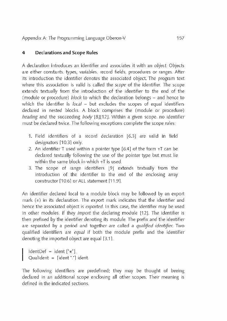
157Appendix A: The Programming Language Oberon_V
4 Declarations and Scope Rules
A declaration introduces an identifier and associates it with an object. Objectsare either constants, types, variables, record fields, procedures or ranges. Afterits introduction the identifier denotes the associated object. The program textwhere this association is valid is called the scope of the identifier. The scopeextends textually from the introduction of the identifier to the end of the(module or procedure) block to which the declaration belongs − and hence towhich the identifier is local − but excludes the scopes of equal identifiersdeclared in nested blocks. A block comprises the (module or procedure)heading and the succeeding body [8][12]. Within a given scope, no identifiermust be declared twice. The following exceptions complete the scope rules:
1. Field identifiers of a record declaration [6.3] are valid in fielddesignators [10.3] only.
2. An identifier T used within a pointer type [6.4] of the form ↑T can bedeclared textually following the use of the pointer type but must liewithin the same block in which ↑T is used.
3. The scope of range identifiers [9] extends textually from theintroduction of the identifier to the end of the enclosing arrayconstructor [10.6] or ALL statement [11.9].
An identifier declared local to a module block may be followed by an exportmark (*) in its declaration. The export mark indicates that the identifier andhence the associated object is exported. In this case, the identifier may be usedin other modules, if they import the declaring module [12]. The identifier isthen prefixed by the identifier denoting its module. The prefix and the identifierare separated by a period and together are called a qualified identifier. Twoqualified identifiers are equal if both the module prefix and the identifierdenoting the imported object are equal [3.1].
IdentDef = ident ["*"].QualIdent = [ident "."] ident.
The following identifiers are predefined; they may be thought of beeingdeclared in an additional scope enclosing all other scopes. Their meaning isdefined in the indicated sections.

158 Appendix A: The Programming Language Oberon_V
ABS [8.2] EXCL [8.2] NEW [6.4]ASL [8.2] FALSE [6.1] ODD [8.2]ASR [8.2] FLOOR [8.2] ORD [8.2]ASSERT [8.2] HALT [8.2] PROD [8.2]BOOLEAN [6.1] IM [8.2] RE [8.2]CEILING [8.2] INC [8.2] REAL [6.1]CHAR [6.1] INCL [8.2] SELECT [8.2]CHR [8.2] INTEGER [6.1] SET [6.1]COMPLEX [6.1] LEN [8.2] SUM [8.2]DEC [8.2] MAX [8.2] TRUE [6.1]EPS [8.2] MIN [8.2] TRUNC [8.2]
5 Constant Declarations
A constant declaration introduces an identifier and associates it with the valueof a constant expression. A constant expression is any expression whoseoperands consist only of literals, set constants, identifiers denoting constants,the predefined identifiers TRUE and FALSE as well as applications of predefinedfunctions to constant expressions.
ConstantDeclaration = IdentDef "=" ConstExpression.ConstExpression = Expression.
Examples:
M = 8N = M*MCR = 0DXpi = 3.14159265all = /{}
6 Type Declarations
A data type determines the set of values which variables of that type mayassume, and the operators that are applicable. A type declaration associates a(type) identifier with a type. There are unstructured and structured types.Unstructured types are either basic types denoted by predefined identifiers,pointer or procedure types. Structured types, namely arrays and records, define

159Appendix A: The Programming Language Oberon_V
also the structure of variables of this type, i.e. the types and possibly the namesof their components.
TypeDeclaration = IdentDef "=" Type.Type = QualIdent | ArrayType | RecordType | PointerType | ProcedureType.
If two (possibly qualified) type identifiers x and y are equal [4] or if they aredeclared to denote equal types in a type declaration of the form x = y, then thetypes T(x) and T(y) denoted by them are equal.
Examples:
Ident = ARRAY 16 OF CHARRealVector = ARRAY OF REALMatrix = ARRAY 100, 100 OF COMPLEXList = RECORD ENDPair = RECORD (List)car, cdr: ↑List
ENDSymbol = RECORDmark: INTEGER;left, right: ↑Symbol;name: ARRAY 32 OF CHAR;bound: ↑List
ENDFunction = PROCEDURE (x: REAL): REAL
6.1 Basic Types
There are 6 basic types in Oberon_V. The corresponding predefined identifiersand the values comprised by its associated types are the following:
BOOLEAN the truth values TRUE and FALSECHAR all characters between 0 and MAX(CHAR)SET all sets containing elements between 0 and MAX(SET)INTEGER all integers between MIN(INTEGER) and MAX(INTEGER)REAL all real numbers between MIN(REAL) and MAX(REAL)COMPLEX all complex numbers x + y * 1.0i with REAL x and y

160 Appendix A: The Programming Language Oberon_V
The last three types are called numeric types and they form a type hierarchy; i.e.values of the smaller type are included by the larger type.
INTEGER L REAL L COMPLEX
6.2 Array Types
An array is a structured type composed of a fixed number of elements which areall of the same type, called the element type. The element type must not be astructured type which is or contains the declared array itself. The number ofelements of an array is called its length. The elements are designated by indiceswhich are integers between 0 and the length minus 1. The number ofdimensions of an array is the number of dimensions of the element type plus 1.A type which is not an array has zero dimensions.
ArrayType = ARRAY [Length {"," Length}] OF Type.Length = ConstExpression.
A declaration of an (n_dimensional) array of the form
ARRAY L1, L2 ... Ln OF T
is an abbreviation of the declaration
ARRAY L1 OFARRAY L2 OF...ARRAY Ln OF T
Arrays declared without length are called open arrays. An open array must not bea component of a type which is not an open array.
Examples:
ARRAY OF CHARARRAY N−1 OF INTEGERARRAY 100, 100 OF COMPLEX

161Appendix A: The Programming Language Oberon_V
6.3 Record Types
A record is a structured type composed of a fixed number of components ofpossibly different types. The record type definition specifies for eachcomponent, called field, its type and an identifier which denotes the field.Within a record declaration, no field identifier must be declared twice. The typeof a field must not be a structured type which is or contains the declared recorditself. If a record type is exported [4], field identifiers that are to be visibleoutside the declaring module must be marked too. They are called public fields;the unmarked components are called private fields.
RecordType = RECORD ["(" BaseType ")"] [FieldList {";" FieldList}] END.BaseType = QualIdent.FieldList = IdentList ":" Type.IdentList = IdentDef {"," IdentDef}.
Record types are extensible, i.e. a record type T1 can be declared as a direct
extension of another record type T which is then called its direct base type. Theextended type T1 consists of the fields of its base type and of the fields whichare declared in T1. A field identifier declared in a (direct) extension must bedifferent from any identifier declared in any of the base type(s) of the record.
T = RECORD ... ENDT1 = RECORD (T) ... END
A record type T1 extends a type T, if it is equal to T or if it directly extends anextension of T. Conversely, a record type T is a base type of T1, if it is equal toT1 or if it is a direct base type of a base type of T1.
Examples:
RECORDhour, min, sec: INTEGER
ENDRECORDname: ARRAY 32 OF CHAR;exported: BOOLEAN;mode: INTEGER;value: REAL
END

162 Appendix A: The Programming Language Oberon_V
6.4 Pointer Types
The pointer type P = ↑T comprises the set of all pointers to variables of type T,and it includes the value NIL which points to no variable at all. The pointer typeis said to be bound to T, and T is called the pointer base type of P. T must be astructured type (i.e. an array or a record type). Two pointer types are equal, iftheir base types are equal.
PointerType = "↑" Type.
If p designates a variable of type ↑T, where T is not an open array type, then acall of the predefined procedure NEW(p) allocates a new variable of type T andthe pointer to it is assigned to p. If p designates a pointer variable bound to ann_dimensional open array, then the call NEW(p, e1, e2, ... en) allocates a newn_dimensional open array variable with lengths given by the values of theexpressions e1, e2, ... en, and the pointer to this array is assigned to p. A variableallocated by NEW is not local to any block.
6.5 Procedure Types
A procedure type P comprises the set of all procedures whose types are equalto P and it includes the value NIL which denotes no procedure at all.
Two procedures have equal types, if all corresponding parameters and theresult types, if any, are equal. Two parameters are equal if they are of the samekind [8.1], if they are denoted by equal identifiers and if they have equal types.
ProcedureType = PROCEDURE [ParameterList].
Examples (see also examples in [6]):
PROCEDUREPROCEDURE (p: ↑List)PROCEDURE (x: COMPLEX): REALPROCEDURE (VAR a: ARRAY OF INTEGER; scale: REAL)PROCEDURE (p: ↑Symbol; cmp: PROCEDURE (x, y: REAL): INTEGER)

163Appendix A: The Programming Language Oberon_V
7 Variable Declarations
Variable declarations introduce new variables by declaring an identifier and atype for them. All variables whose identifiers appear in the same identifier listhave equal types. The type of a variable (which is not a parameter) must not bean open array [6.2]. A structured variable is a variable which has a structuredtype [6]. It consists of component variables (i.e. array elements or record fields)as specified by its type.
VariableDeclaration = IdentList ":" Type.
Record variables have both a static and a dynamic type. The former is the typewith which they are declared and which is simply called their type; the latter isthe type which their values may assume at run_time. Variable parameters ofrecord type and record variables referred to by pointers may have a dynamictype which is an extension of their static type.
Examples (see also examples in [5] and [6]):
ch: CHARi, j, k: INTEGERx, y: REALu, v: COMPLEXok: BOOLEANs: SETf: FunctionA: Matrixp, q: ↑Pairroot: ↑Symbolindex: ARRAY 100 OF INTEGERa, b, c: ARRAY N OF REALid: Ident
8 Procedure Declarations
A procedure declaration consists of two parts, a procedure heading and a body.The heading specifies the procedure identifier and the procedure type(determined by the parameters and the result type, if any). The body containsdeclarations and statements that are executed, when the procedure is called.

164 Appendix A: The Programming Language Oberon_V
The procedure identifier must be repeated at the end of the proceduredeclaration.
ProcedureDeclaration = ProcedureHeading ";" Body END ident.ProcedureHeading = PROCEDURE IdentDef [ParameterList].ForwardDeclaration = PROCEDURE "↑" IdentDef [ParameterList].Body = DeclarationSequence [BEGIN StatementSequence].DeclarationSequence =[CONST {ConstDeclaration ";"}][TYPE {TypeDeclaration ";"}][VAR {VarDeclaration ";"}]{ProcedureDeclaration ";" | ForwardDeclaration ";"} .
All objects declared in a procedure body are local to it [4]. Values of localvariables are undefined upon entry to a procedure. Objects declared in theenvironment of the procedure are also visible within the procedure, with theexception of those objects that have equal identifiers as locally declared objects.The use of the procedure identifier in a call within its declaration impliesrecursive activation of the procedure.
Procedures are either proper procedures or function procedures. The formerrepresent an (abstract) action while the latter compute a value. The execution ofa function procedure must terminate with an explicit RETURN statement [11.9]which also denotes the value to be returned. The result type cannot be astructured type. Function procedures must produce no side effects; i.e. within afunction procedure the following restrictions apply:
1. no value must be assigned to a variable which is not local, and2. no proper procedure (except predefined ones) must be called.
A procedure identifier may be introduced by a forward declaration. In this case,the scope of the procedure identifier extends from its introduction to the end ofthe block to which the forward declaration belongs. The actual declarationcontaining the procedure body must follow later within the same block. Theprocedure types of both declarations must be equal [6.5].

165Appendix A: The Programming Language Oberon_V
8.1 Parameters
Parameters are identifiers declared in a parameter section of a procedureheading. They are local to the procedure block and they denote the argumentsspecified in the procedure call. The association between parameters andarguments is established, when the procedure is called.
There are two kinds of parameters, namely value and variable parameters,indicated in the parameter section by the absence or presence of the reservedword VAR. Value parameters denote local variables to which the value of theassociated argument is assigned as initial value. Variable parameters areassociated with arguments that must be variables and they denote thesenon_local variables (i.e. a variable parameter is a local identifier for a non_localvariable).
ParameterList = "(" [ParameterSection {";" ParameterSection}] ")" [":" Type].ParameterSection = [VAR] ident {"," ident} ":" Type.
The types of the parameters (i.e. the types of the variables denoted by theparameters) are specified in the parameter sections; all parameters whichappear in the same parameter section are of the same parameter kind and haveequal types. The type of value parameters cannot be a structured type.
Examples of procedure declarations (see also examples of [6]):
PROCEDURE ReadInt (VAR x: INTEGER);VAR n, s: INTEGER; ch: CHAR;
BEGIN s := 0; n := 0; Read(ch);WHILE ch < 80X DO INC(n, ASL(ORD(ch), s)); INC(s, 7); Read(ch) END;x := n + ASL(ORD(ch) − 192, s)
END ReadInt
PROCEDURE WriteInt (x: INTEGER);BEGINWHILE (x < −64) OR (x > 63) DOWrite(CHR(x MOD 128)); x := x DIV 128
END;Write(R, CHR(x + 192))
END WriteInt

166 Appendix A: The Programming Language Oberon_V
PROCEDURE saxpy (a: REAL; VAR x, y: RealVector);BEGIN ALL i = 0 .. LEN(x)−1 DO y[i] := a * x[i] + y[i] ENDEND saxpy
PROCEDURE Size (p: ↑Symbol): INTEGER;BEGINIF p = NIL THEN RETURN 0ELSE RETURN 1 + Size(p.left) + Size(p.right)END
END Size
8.2 Predefined Procedures
The following tables list the predefined procedures. Some of them are generic,i.e. they apply to several types of arguments. x, y and n stand for expressions, vstands for a variable and T for a type.
Function procedures:
Call Argument types Result type Function
ABS(x) INTEGER INTEGER absolute value of xREAL REALCOMPLEX REAL
ASL(x, n) x, n: INTEGER INTEGER x * 2n (n 3 0)ASR(x, n) x, n: INTEGER INTEGER x DIV 2n (n 3 0)ODD(x) INTEGER BOOLEAN x MOD 2 = 1ORD(x) CHAR INTEGER ordinal number of xCHR(x) INTEGER CHAR x = CHR(ORD(x))EPS(x) REAL REAL small. real e: x + e > xTRUNC(x) REAL INTEGER integer part of xFLOOR(x) REAL INTEGER largest integer i with i # xCEILING(x) REAL INTEGER small. integer i with i 3 xRE(x) COMPLEX REAL real part of xIM(x) COMPLEX REAL imaginary part of xLEN(v, n) v: array INTEGER length of v in dim. n
n: INTEGERLEN(v) v: array INTEGER LEN(v) = LEN(v, 0)MIN(T) CHAR CHAR 0X
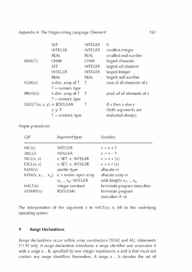
167Appendix A: The Programming Language Oberon_V
SET INTEGER 0INTEGER INTEGER smallest integerREAL REAL smallest real number
MAX(T) CHAR CHAR largest characterSET INTEGER largest set elementINTEGER INTEGER largest integerREAL REAL largest real number
SUM(x) n_dim. array of T T sum of all elements of vT = numeric type
PROD(x) n_dim. array of T T prod. of all elements of vT = numeric type
SELECT(n, x, y) n: BOOLEAN T if n then x else yx, y: T (both arguments areT = unstruct. type evaluated always)
Proper procedures:
Call Argument types Function
INC(v) INTEGER v := v + 1DEC(v) INTEGER v := v − 1INCL(v, x) v: SET; x: INTEGER v := v + {x}EXCL(v, x) v: SET; x: INTEGER v := v / {x}NEW(v) pointer type allocate v↑NEW(v, x1, ... xn) v: ↑ n_dim. open array allocate array v↑
x1, ... xn: INTEGER with lengths x1, ... xnHALT(n) integer constant terminate program executionASSERT(n) BOOLEAN terminate program
execution if ˜n
The interpretation of the argument x in HALT(x) is left to the underlyingoperating system.
9 Range Declarations
Range declarations occur within array constructors [10.6] and ALL statements[11.9] only. A range declaration introduces a range identifier and associates itwith a range a .. b, specified by two integer expressions a and b that must notcontain any range identifiers themselves. A range a .. b denotes the set of
168 Appendix A: The Programming Language Oberon_V
integers between a and b (inclusive). The number of integers denoted by arange is called its length. A range declaration that introduces n range identifiersis called n_dimensional. A range identifier may be used within an expression[10.3].
RangeDeclaration = RangeList {"," RangeList}.RangeList = ident {"," ident} "=" Range.Range = Expression ".." Expression.
An (n_dimensional) range declaration of the form
r1, r2, ... rn = a .. b
is an abbreviation of the declaration
r1 = a .. b, r2 = a .. b, ... rn = a .. b
Examples:
r = M .. Ni, j, k = 0 .. LEN(A)−1i = 1 .. M, j = 1 .. Ni, j = −10 .. 10
10 Expressions
An expression specifies the computation of a value; it consists of operands andoperators. The value of the expression is determined by applying the operatorsaccording to their precedences to the values of the operands. Operands areeither literals, sets, designators, function calls or expressions.
10.1 Literals
Literals are numbers, character constants, strings and the value NIL. The value ofa literal is the value it represents.
Literal = number | character | string | NIL.

169Appendix A: The Programming Language Oberon_V
10.2 Sets
A set represents a value of type SET by listing its elements between braces. Theelements must be integer values. The notation a .. b is an abbreviation for theelements a, a+1, .. b. A set constant is a set where all elements are denoted byconstant expressions.
Set = "{" [Element {"," Element}] "}".Element = Expression [".." Expression].
Examples:
{0, 4, 10} {i} {0 .. i} {i .. i+4, 42}
10.3 Designators
A designator is a qualified identifier [4] possibly followed by selectors or typeguards. The value of a designator denoting a constant is the value of theconstant. The value of a designator denoting a type or procedure is the denotedtype or procedure. A designator denoting a variable stands for this variable.Within an array constructor [10.6] or an ALL statement [11.9], a range identifierdenotes any integer value within the associated range.
Designator = QualIdent {"[" ExpressionList "]" | "." | "↑" | "{" QualIdent "}"}.ExpressionList = Expression {"," Expression}.
If A designates an array variable, then A[e] denotes the element of A whoseindex is the current value of the expression e. A designator of the formA[e1][e2] ... [en] may be abbreviated to A[e1, e2, ... en]. IF p designates a pointervariable, then p↑ denotes the variable which is referenced by p. If r designates arecord variable, then r.f denotes the field f of r. Designators of the forms p↑.fand p↑[e] may be abbreviated to p.f and p[e] respectively.
If the variable v is of record type [6.3], the type guard v{T} asserts that thedynamic type of v is an extension of T. If v is a pointer type [6.4], v{T} assertsthat the dynamic type of v↑ is an extension of T. The static type of thedesignator v{T} is then T (or ↑T respectively). If the assertion fails, the programexecution is aborted. The type guard is applicable, if

170 Appendix A: The Programming Language Oberon_V
1. v is a record variable parameter or v is a pointer (v 9 NIL), and if2. the record type T is an extension of the static type of v (or v↑
respectively).
Examples (see also examples in [7]):
Designator Type
i INTEGERA[i, 10] COMPLEXp.car↑ Listq.cdr{Pair} ↑Pairroot.name[k] CHARf Function
10.4 Function Calls
A function call activates a function procedure [8]. The value of a function call isthe value returned by the function procedure. The call consists of a designatordenoting a function procedure followed by a possibly empty list of arguments[10.5].
FunctionCall = Designator "(" [ArgumentList] ")".
Examples (see also examples in [7]):
f(x*pi)Size(root)TRUNC(x*x + y*y)
10.5 Arguments
Within a procedure, the arguments are denoted by their correspondingparameters specified in the procedure declaration. The correspondence isdetermined by the positions of the arguments and parameters within theargument and parameter list.

171Appendix A: The Programming Language Oberon_V
ArgumentList = Argument {"," Argument}.Argument = Expression | ArrayConstructor .
There are two kinds of parameters, namely value and variable parameters [8.1].In case of a value parameter, the corresponding argument must be anexpression. This expression is evaluated prior to the procedure call and theresulting value is assigned to the value parameter. Argument and parametermust observe the rules for assignments.
In case of a variable parameter, the corresponding argument must be adesignator or an array constructor [10.6] both denoting a variable, or a string(since value parameters cannot have a structured type [8.1]). The parameter andthe argument type must be equal, except for record and open array parameters,where the following rules apply:
1. If the type of the parameter is a record [6.3], the type of the argumentmust be an extension of the parameter's type. After procedureactivation, the dynamic type of the parameter corresponds to thedynamic type of the argument.
2. If the type of the parameter is an open ARRAY OF T [6.2], the type ofthe argument may be any array with element type T1, where T and T1are equal or the types T and T1 themselves observe this rule (with T asparameter type and T1 as argument type).
3. If the type of the parameter is ARRAY OF CHAR, the argument may bea string. The string is copied into an (anonymous) array variable whichis passed as argument instead.
10.6 Array Constructors
An array constructor is a range declaration [9] followed by an expression. Anarray constructor consisting of an n_dimensional range declaration specifies anarray [6.2] with at least n dimensions. The range identifiers correspond to thedimensions of the array in the order of their occurence in the range declaration.The array lengths in each dimension are the lengths of the correspondingranges.
ArrayConstructor = "[" RangeDeclaration ":" Expression "]".

172 Appendix A: The Programming Language Oberon_V
An array constructor of the form
[r1 = ..., r2 = ..., ... rn = ... : E(r1, r2, ... rn)]
denotes an array of type ARRAY l1, l2, ... ln OF T, where the lk's are the lengths ofthe ranges associated with the range identifiers rk (1 # k # n) and T is the typeof the expression E. The array element denoted by the indices i1, i2, ... in is theelement E(i1, i2, ... in), i.e. the value of the expression E(i1, i2, ... in) which isobtained when all range identifiers rk are substituted by ik (1 # k # n). Thenumber of dimensions of the constructed array is n plus the number ofdimensions of the element type T.
If E(r1, r2, ... rn) is a designator denoting a variable, then the array constructordenotes an array variable. Array variables may be used as arguments for openarray parameters [10.5]. The following restrictions apply to designators E(r1, r2,... rn) of array variable constructors:
1. Only a restricted form of designators is allowed, namely designatorsobserving the following syntactic production:
ArrayDesignator = QualIIdent {"[" ExpressionList "]" | "."}
2. An expression in the expression list of such a designator must eithercontain no range identifier at all, or it must be transformable into theform r*x + y where r is a range identifier and x and y contain no rangeidentifiers (i.e. the expression must be linear in r).
3. None of the index expressions containing a range identifier r mustdenote the same (constant) value for all values of r (i.e. x must not bezero in the expression r*x + y; cf. rule 2).
4. All range identifiers introduced by the preceeding range declarationmust be used at least once in the designator.
If E(r1, r2, ... rn) is an expression denoting a value, then the array constructordenotes an array value. Array values may be used as arguments for thepredefined procedures SUM and PROD only.
Examples (see also examples in [7]):
Array constructor Denoted Array
[i = 0 .. 3: id[2*i + 1]] elements id[1], id[3], id[5], id[7] (variable)

173Appendix A: The Programming Language Oberon_V
[j = 0 .. LEN(A)−1: A[j, j]] diagonal of A (variable)[k = 0 .. N−1: a[k] * b[k]] elementwise product of a and b (value)
10.7 Operators
Operators are special characters, character pairs or reserved words [3.5]denoting unary and binary operations. The operation denoted by an operatormay depend on the type(s) of its operand(s). There are 4 different precedenceclasses for operators. The operator ˜ has the highest precedence, followed bythe multiplication operators, the addition operators and the relations. Operatorsof the same precedence associate from left to right; e.g. x−y−z is anabbreviation for (x−y)−z.
Expression = SimpleExpression [Relation SimpleExpression].Relation = "=" | "#" | "<" | "<=" | ">" | ">=" | IN | IS.SimpleExpression = ["−"] Term {AddOperator Term}.AddOperator = "+" | "−" | "%" | "|".Term = ["/"] Factor {MulOperator Factor}.MulOperator = "*" | "/" | DIV | MOD | "&".Factor =Literal | Set | Designator | FunctionCall | "˜" Factor | "(" Expression ")".
10.7.1 Arithmetic Operators
The operators +, −, * and / apply to operands of numeric types [6.1]. The resulttype is the smallest type which includes the types of both operands, except fordivision (/), where the result type includes the type REAL too. The expression0−e may be abbreviated to −e.
Symbol Result
+ sum− difference* product/ quotientDIV integer quotientMOD modulus

174 Appendix A: The Programming Language Oberon_V
The operators DIV and MOD apply to integer operands only. For any dividend xand positive divisor y the following relationships hold:
x : (x DIV y) * y + x MOD y0 # x MOD y < y
10.7.2 Logical Operators
Logical operators apply to boolean operands [6.1] and yield a boolean result.The evaluation of the operands of & and | proceeds from left to right and onlyas many operands are evaluated as necessary for the determination of theresult.
Symbol Result Description
| disjunction p | q : if p then TRUE else q& conjunction p & q : if p then q else FALSE˜ negation ˜p : not p
10.7.3 Set Operators
Set operators apply to operands of type SET [6.1] and yield a result of this type.A set expression of the form {0 .. MAX(SET)} / x may be abbreviated to /x. Notethat x / y : x * (/y).
Symbol Result Description
+ union x IN s + t : (x IN s) | (x IN t)* intersection x IN s * t : (x IN s) & (x IN t)/ difference x IN s / t : (x IN s) & ˜(x IN t)% symmetric difference x IN s % t : (x IN s) # (x IN t)

175Appendix A: The Programming Language Oberon_V
10.7.4 Relations
Relations yield a boolean result [6.1]. The ordering relations <, <=, > and >=apply to operands of type CHAR, INTEGER and REAL [6.1] as well as tocharacter arrays [6.2] and strings [3.4]. The relations = and # apply to allunstructured types [6] (including the value NIL) as well as to character arraysand strings. x IN s tests whether x is an element of s. x must be of typeINTEGER and s of type SET.
Symbol Relation
= equal# unequal< less<= less or equal> greater>= greater or equalIN element testIS type test
If the variable v is of record type [6.3], the type test v IS T holds if the dynamictype of v is an extension of T. If v is a pointer type [6.4], v IS T holds if thedynamic type of v↑ is an extension of T. The type test is applicable, if
1. v is a record variable parameter or v is a pointer (v 9 NIL), and if2. the record type T is an extension of the static type of v (or v↑
respectively).
Examples (see also examples in [7]):
Expression Type
ch CHAR1993 INTEGERi + j DIV 2 INTEGERs / {0 .. 9, k} SETi + j / k REALx * (−y) + k REALf(i * x + 1.0E−3) REAL(u + v) * 1.0i COMPLEX

176 Appendix A: The Programming Language Oberon_V
2*(u + RE(v)) COMPLEX˜ok | (i # j) BOOLEAN('a' <= ch) & (ch <= 'z') BOOLEANroot.name < "lambda" BOOLEANk IN {i .. j−1} BOOLEANp.car IS Pair BOOLEAN
11 Statements
A statement denotes an action. Executing a statement means performing thedenoted action. There are elementary statements and structured statements. Theformer are not composed of any parts that are themselves statements. They arethe assignment, the procedure call and the return statement. Structuredstatements are composed of parts that are themselves statements; they areused to express conditional, repetitive or parallel execution of its componentstatements.
Let P and Q be predicates denoting the program states before and after theexecution of a statement S; i.e. P denotes a precondition of S and Q denotes apostcondition. Then the predicate {P} S {Q} holds, if P holds before theexecution of S, S terminates and Q holds after the execution of S. An axiom of astructured statement S specifies rules for its component statements Si and thepredicates P and Q, such that {P} S {Q} holds.
Statement =Assignment | ProcedureCall | ReturnStatement |IfStatement | CaseStatement |WhileStatement | RepeatStatement | AllStatement.
11.1 Statement Sequences
A statement sequence denotes sequential execution of the componentstatements. Any two textually consecutive statements must be separated by asemicolon; the statement before the semicolon is executed before thestatement following the semicolon. An empty statement sequence denotes noaction at all.
StatementSequence = [Statement {";" Statement}].

177Appendix A: The Programming Language Oberon_V
Axiom of statement sequences:
{P} S1; S2; ... Sn {Q}
holds if there exist conditions Pi and Qi such that
R i : 1 # i # n : {P i} Si {Qi}R i : 1 < i # n : Qi−1 ↑ PiP ↑ P1Qn↑ Q
11.2 Assignments
The execution of an assignment replaces the current value of a variable [7] bythe value of the specified expression [10].
Assignment = Designator ":=" Expression.
The type T(v) of the variable v in an assignment of the form v := e must be anunstructured type [6] or a character array [6.2], and one of the followingconditions must hold for T(v) and the type of the expression T(e):
1. T(v) and T(e) are equal; or2. T(v) and T(e) are numerical types and T(v) includes T(e); or3. T(v) and T(e) are pointer types and the pointer base type of T(e) is an
extension of the pointer base type of T(v), or4. T(v) is a pointer or procedure type and e is NIL, or5. T(v) is a character array and T(e) is a character array or e is a string.
Then, e is copied to v and, if necessary, e is shortened to the length ofv. The character sequence in v is always terminated by the character0X.
Examples (see also examples in [7]):
ch := CRi := 0x := RE(u)y := 1 + x*pik := Size(root)

178 Appendix A: The Programming Language Oberon_V
u := u / ABS(u)ok := (i < j) & (k IN {i .. j})A[i, j] := A[i, k] * vp := NILq := q.cdr{Pair}root.left.name[0] := 0X
11.3 Procedure Calls
The execution of a procedure call activates the designated procedure. The callconsists of a designator denoting a proper procedure [8] possibly followed by alist of arguments [10.5].
ProcedureCall = Designator ["(" ArgumentList ")"].
Examples (see also examples in [7] and [8]):
ReadInt(i)WriteInt(ORD(ch))saxpy(x, [i = 10 .. 20: a[i]], [i = 10 .. 20: b[i]])INC(root.mark)EXCL(s, 0)
11.4 RETURN Statement
A RETURN statement consists of the symbol RETURN, possibly followed by anexpression. It indicates the termination of a procedure, and the expressionspecifies the result of a function procedure. Its type must be equal to the resulttype specified in the procedure heading. The expression and the result typemust observe the rules for assignments.
ReturnStatement = RETURN [Expression].
Function procedures require the presence of a RETURN statement indicating theresult value. There may be several, although only one will be executed. Inproper procedures, a RETURN statement is implied by the end of the procedurebody. An explicit RETURN statement therefore appears as an additional(probably exceptional) termination point.

179Appendix A: The Programming Language Oberon_V
11.5 IF Statement
The IF statement specifies the conditional execution of guarded statements. Thestatement sequence following the symbol THEN is executed if the precedingboolean expression (guard) evaluates to true, otherwise the statement sequencefollowing the symbol ELSE is executed, if there is one.
IfStatement =IF Expression THEN StatementSequence{ELSIF Expression THEN StatementSequence}[ELSE StatementSequence]END.
An IF statement of the form
IF B1 THEN S1ELSIF B2 THEN S2...ELSIF Bn THEN SnELSE S0END
is an abbreviation for
IF B1 THEN S1ELSEIF B2 THEN S2ELSE...
ELSE Bn THEN SnELSE S0END
...END
END

180 Appendix A: The Programming Language Oberon_V
Axiom of the IF statement:
{P} IF B THEN S1 ELSE S2 END {Q}
holds if there exist conditions P1 and P2 such that
{P1} S1 {Q}{P2} S2 {Q}P Y B ↑ P1P Y XB ↑ P2
Example:
IF ('0' <= ch) & (ch <= '9') THEN d := ORD(ch) − ORD('0')ELSIF ('A' <= ch) & (ch <= 'F') THEN d := ORD(ch) − ORD('A')ELSE Error; d := 0END
11.6 CASE Statement
A CASE statement specifies the conditional execution of a statement sequenceselected by the value of an expression. After evaluation of the expression, thestatement sequence is executed, whose case label list contains the obtainedvalue. The case expression and all case labels must be of the same type whichmust be CHAR or INTEGER. Case labels must be constant expressions and novalue must occur more than once. If the value of the case expression does notoccur as a label of any case, the statement sequence following the symbol ELSEis executed, if there is one. Otherwise the program is aborted.
CaseStatement =CASE Expression{OF CaseLabelList THEN StatementSequence}[ELSE StatementSequence]END.
CaseLabelList = CaseLabels {"," CaseLabels}.CaseLabels = ConstExpression [".." ConstExpression].

181Appendix A: The Programming Language Oberon_V
Axiom of the CASE statement (each ki stands for a single case label):
{P}CASE kOF k1 THEN S1OF k2 THEN S2...OF kn THEN SnELSE S0END{Q}
holds, if there exist conditions Pi such that
R i : 0 # i # n : {P i} Si {Q}R i : 0 < i # n : P Y (k = k i) ↑ PiR i : 0 < i # n : P Y (k 9 k i) ↑ P0
Example:
CASE chOF '(' THEN sym := lparenOF 27X THEN sym := quoteOF ')' THEN sym := rparenOF '.' THEN sym := periodOF '0' .. '9' THEN NumberOF 'A' .. 'Z', 'a' .. 'z' THEN IdentifierELSE sym := nullEND
11.7 WHILE Statement
A WHILE statement specifies the repeated execution of a statement sequenceas long as the preceding boolean expression (guard) evaluates to true. Thestatement sequence may not be executed at all.
WhileStatement = WHILE Expression DO StatementSequence END.

182 Appendix A: The Programming Language Oberon_V
Axiom of the WHILE statement:
{P} WHILE B DO S END {Q}
holds if an invariant H exists such that
P ↑ H{H Y B} S {H}H Y XB ↑ Q
Examples:
WHILE x > 0 DOIF ODD(x) THEN INC(i) END;x := x DIV 2
END
WHILE (q # NIL) & (q.name # name) DO p := q; q := q.next END
11.8 REPEAT Statement
The REPEAT statement specifies the repeated execution of a statementsequence until a condition is satisfied. The statement sequence is executed atleast once.
RepeatStatement = REPEAT StatementSequence UNTIL Expression.
Axiom of the REPEAT statement:
{P} REPEAT S UNTIL B {Q}
holds if there exists an invariant H such that
{P} S {H}{H Y XB} S {H}H Y B ↑ Q

183Appendix A: The Programming Language Oberon_V
Example:
REPEATd[i] := ORD(x MOD 10 + ORD('0'));x := x DIV 10; INC(i)
UNTIL x = 0
11.9 ALL Statement
The ALL statement specifies the potentially parallel execution of a set ofassignment sequences determined by an n_dimensional range declaration [9]which preceds the assignments. For each element of the set R = {(i1, i2, ... in) :(ik N ran(rk)) Y (1 # k # n)} where ran(rk) is the range associated with the rangeidentifier rk, the assignment sequence is executed exactly once. For a particularassignment sequence, the range identifier rk stands for the value ik of theelement (i1, i2, ... in) corresponding to that assignment sequence.
AllStatement = ALL RangeDeclaration DO AssignmentSequence END.AssignmentSequence = [Assignment {";" Assignment}].
Let i denote (i1, i2, ... in) for short. If S(i) denotes a particular assignmentsequence (i.e. the assignment sequence corresponding to the element (i1, i2, ...in) N R), then S(i) must be independent of any other assignment sequence S(j)with i 9 j; i.e. the order in which a range identifier rk assumes a value within itsassociated range ran(rk) is unspecified. To be precise, let in(i) be the set ofvariables accessed by S(i) and out(i) be the set of variables to which valueshave been assigned to by S(i). Then, for any two different elements i, j N R thefollowing must hold:
1. in(i) G out(j) must be the empty set, and2. out(i) G out(j) must be the empty set.
Axiom of the ALL statement:
{P} ALL i N R DO S(i) END {Q}
holds if conditions Pi and Qi exist such that

184 Appendix A: The Programming Language Oberon_V
P ↑ (R i : i N R : Pi)R i : i N R : {Pi} S(i) {Qi}(R i : i N R : Qi) ↑ Q
and
R i, j : i, j N R, i 9 j : (in(i) G out(j) = F) Y (out(i) G out(j) = F)
with in(i) : set of variables that have been accessed by S(i)and out(i) : set of variables to which values have been assigned to by S(i)
Examples (see also examples in [7]):
ALL i = 0 .. LEN(c)−1 DO c[i*2] := i * pi ENDALL i = j .. k DO a[j] := SELECT(a[j] > 0, a[j], 0) * b[j] ENDALL i, j = 0 .. LEN(A)−1 DO A[i, j] := 1/(i+j+1) ENDALL r = 10 .. 20 DO a[r] := a[index[r]]; a[index[r]] := 0 END
12 Modules
A module is a collection of declarations of objects and a sequence ofstatements for the purpose of assigning initial values to variables. A moduleconstitutes a text that is compilable as a unit.
A module consists of a module heading and a body. The heading defines themodule identifier and possibly imported modules. The body containsdeclarations and statements that are executed, when the module is added to asystem (loaded). The module identifier must be repeated at the end of themodule specification.
Module = ModuleHeading ";" Body END ident ".".ModuleHeading = MODULE ident [ImportList].ImportList = "(" Import {"," Import} ")".Import = Ident [":=" ident].
The import list specifies the modules which are imported and hence of whichthe importing module is a client. If an identifier x is exported [4] by a moduleM, and M appears in a module's import list, then x is referred to as M.x withinthe importing module. An import of the form M1 := M may be used to (locally)substitute the module identifier M by M1. An identifier x exported by the

185Appendix A: The Programming Language Oberon_V
module M is then referred to as M1.x within the importing module.The values of global variables are undefined upon loading of the module.
The statements in bodies of imported modules are executed before anystatement of the importing module is executed.
Example:
MODULE Out (Unix);
CONST maxLen = 80;VAR len: INTEGER;
PROCEDURE Ln*;BEGIN Unix.Put(0AX); Unix.Flush; len := 0END Ln;
PROCEDURE Char* (x: CHAR);BEGINIF len = maxLen THEN Ln END;Unix.Put(ch); INC(len)
END Char;
PROCEDURE String* (VAR s: ARRAY OF CHAR);VAR i: INTEGER;
BEGIN i := 0;WHILE (i < LEN(s)) & (s[i] # 0X) DO Char(s[i]); INC(i) END
END String;
PROCEDURE Int* (x: INTEGER);VAR i: INTEGER; d: ARRAY 16 OF CHAR;
BEGIN i := 0;IF x < 0 THEN x := −x; Char('−') END;REPEAT d[i] := CHR(x MOD 10 + 30H); x := x DIV 10; INC(i)UNTIL x = 0;REPEAT DEC(i); Char(d[i]) UNTIL i = 0
END Int;

186 Appendix A: The Programming Language Oberon_V
PROCEDURE Set* (s: SET);VAR i, j: INTEGER;
BEGINChar('{'); j := 0;WHILE s # {} DOIF j IN s THEN i := j;REPEAT EXCL(s, j); INC(j) UNTIL (s = {}) | ˜(j IN s);Int(i);IF i+2 = j THEN String(", "); Int(j−1)ELSIF i+2 < j THEN String(" .. "); Int(j−1)END;IF s # {} THEN String(", ") END
END;INC(j)
END;Char('}')
END Set;
BEGIN Unix.Init; len := 0END Out.
12.1 The Module SYSTEM
The module SYSTEM provides procedures that are necessary to program certainlow level operations and to circumvent the type system of Oberon_V. A moduleimporting SYSTEM must be considered to be inherently unsafe andnon_portable; therefore SYSTEM should be used very restrictively. Although theoperations provided by it are machine specific and hence may vary frommachine to machine, the following procedures are assumed to be found inevery SYSTEM implementation. x, y and n stand for expressions, v stands for avariable and T for a type.
Function procedures:
Call Argument types Result type Function
ADR(v) any type INTEGER address of variable vLSL(x, n) INTEGER INTEGER logical shift left by n bitsLSR(x, n) INTEGER INTEGER logical shift right by n bits

187Appendix A: The Programming Language Oberon_V
SIZE(T) any type INTEGER space required by TVAL(T, x) any type type of T x interpreted as of type T
Proper procedures:
Call Argument types Function
GET(a, v) a: INTEGER; v := Mem[a]v: any unstructured type
PUT(a, x) a: INTEGER; Mem[a] := xv: any unstructured type
MOVE (x, y, n) INTEGER ALL i = 0 .. n−1 DOMem[y+i] := Mem[x+i]
ENDNEW(v, n) v: any pointer type allocate storage block of n
n: integer type words and assign itsaddress to v


Appendix B:
Program Examples
The following program examples shall demonstrate the usage of ALLstatements and of array constructors. The BLA routines as well as the Linpackprocedures have been adapted from [Dongarra 1979].
1 BLAS
Module OVBlas contains five of the most frequently used BLA subroutines. Thismodule has been used for the measurements in Section 6.1.
MODULE OVBlas;
TYPE
RealVector* = ARRAY OF REAL;
PROCEDURE isamax* (VAR x: RealVector): INTEGER;
VAR i, j: INTEGER; max: REAL;
BEGIN max := ABS(x[0]); i := 0; j := 1;
WHILE j < LEN(x) DO
IF ABS(x[j]) > max THEN max := ABS(x[j]); i := j END;
INC(j)
END;
RETURN i
END isamax;
PROCEDURE sscal* (a: REAL; VAR x: RealVector);
BEGIN ALL i = 0 .. LEN(x)−1 DO x[i] := a * x[i] END
END sscal;

190 Appendix B: Program Examples
PROCEDURE saxpy* (a: REAL; VAR x, y: RealVector);
BEGIN
ASSERT(LEN(x) = LEN(y));
ALL i = 0 .. LEN(x)−1 DO y[i] := a * x[i] + y[i] END
END saxpy;
PROCEDURE sasum* (VAR x: RealVector): REAL;
BEGIN RETURN SUM([i = 0 .. LEN(x) − 1: ABS(x[i])])
END sasum;
PROCEDURE sdot* (VAR x, y: RealVector): REAL;
BEGIN RETURN SUM([i = 0 .. LEN(x) −1: x[i] * y[i]])
END sdot;
END OVBlas.
2 Linpack
Module OVLinpack1 contains a one_to_one translation of the Linpackprocedures sgefa and sgesl. They are used to solve general systems ofsimultaneous linear algebraic equations. For a detailed discussion of thealgorithms the reader is referred to [Dongarra 1979].
MODULE OVLinpack1 (Blas := OVBlas);
TYPE
IntVector* = ARRAY OF INTEGER;
RealVector* = Blas.RealVector;
RealMatrix* = ARRAY OF RealVector;
PROCEDURE sgefa* (VAR a: RealMatrix; VAR ipvt: IntVector; VAR info: INTEGER);
VAR
j, k, kp1, l, n, nm1: INTEGER;
t: REAL;
BEGIN
info := −1; n := LEN(a); nm1 := n−1;
IF nm1 >= 1 THEN k := 0;
WHILE k < nm1 DO kp1 := k+1;
(* find l = pivot index *)
l := Blas.isamax([i = k .. nm1: a[i, k]]) + k;
ipvt[k] := l;
(* zero pivot implies this column already triangularized *)
IF a[l, k] # 0 THEN
(* interchange if necessary *)
IF l # k THEN t := a[l, k]; a[l, k] := a[k, k]; a[k, k] := t END;

191Appendix B: Program Examples
(* compute multipliers *)
t := −1/a[k, k];
Blas.sscal(t, [i = kp1 .. nm1: a[i, k]]);
(* row elimination with column indexing *)
j := kp1;
WHILE j < n DO t := a[l, j];
IF l # k THEN a[l, j] := a[k, j]; a[k, j] := t END;
Blas.saxpy(t, [i = kp1 .. nm1: a[i, k]], [i = kp1 .. nm1: a[i, j]]);
INC(j)
END
ELSE info := kp1
END;
k := kp1
END
END;
ipvt[nm1] := nm1;
IF a[nm1, nm1] = 0 THEN info := n END
END sgefa;
PROCEDURE sgesl*
(VAR a: RealMatrix; VAR ipvt: IntVector; VAR b: RealVector; job: INTEGER);
VAR
n, k, kb, l, nm1: INTEGER;
t: REAL;
BEGIN
n := LEN(a); nm1 := n−1;
IF job = 0 THEN
(* solve a * x = b; first solve l * y = b *)
IF nm1 >= 1 THEN k := 0;
WHILE k < nm1 DO
l := ipvt[k]; t := b[l];
IF l # k THEN b[l] := b[k]; b[k] := t END;
Blas.saxpy(t, [i = 1 .. n−k−1: a[k+i, k]], [i = 1 .. n−k−1: b[k+i]]);
INC(k)
END
END;
(* now solve u * x = y *)
kb := 0;
WHILE kb < n DO
k := n − 1 − kb;
b[k] := b[k] / a[k, k];
t := −b[k];
Blas.saxpy(t, [i = 0 .. k−1: a[i, k]], [i = 0 .. k−1: b[i]]);
INC(kb)
END
ELSE
(* solve trans(u) * x = b; first solve trans(u) * y = b *)
k := 0;

192 Appendix B: Program Examples
WHILE k < n DO
t := Blas.sdot([i = 0 .. k−1: a[i, k]], [i = 0 .. k−1: b[i]]);
b[k] := (b[k] − t) / a[k, k];
INC(k)
END;
(* now solve trans(l) * x = y *)
IF nm1 >= 1 THEN kb := 0;
WHILE kb < nm1 DO
k := n − 1 − kb;
b[k] := Blas.sdot([i = 1 .. n−k−1: a[k+i, k]], [i = 1 .. n−k−1: b[k+i]]) + b[k];
l := ipvt[k];
IF l # k THEN t := b[l]; b[l] := b[k]; b[k] := t END;
INC(kb)
END
END
END
END sgesl;
END OVLinpack1.
Module OVLinpack2 contains the same procedures as OVLinpack1, but with"inlined" ALL statements instead of the BLAS calls. Because the BLA proceduresreduce to simple "one_liners" when using ALL statements, this leads to a betterreadable program (only the procedure sgefa is shown). This module has beenused for the measurements in Section 6.2.
MODULE OVLinpack2 (Blas := OVBlas);
TYPE
IntVector* = ARRAY OF INTEGER;
RealVector* = Blas.RealVector;
RealMatrix* = ARRAY OF RealVector;
PROCEDURE sgefa* (VAR a: RealMatrix; VAR ipvt: IntVector; VAR info: INTEGER);
VAR j, k, l, n: INTEGER; t: REAL;
BEGIN
info := −1; n := LEN(a);
IF n > 1 THEN k := 0;
WHILE k < n−1 DO;
(* find l = pivot index *)
l := Blas.isamax([i = k .. n−1: a[i, k]]) + k ;
ipvt[k] := l;
(* zero pivot implies this column already triangularized *)
IF a[l, k] # 0 THEN
(* interchange if necessary *)
IF l # k THEN t := a[l, k]; a[l, k] := a[k, k]; a[k, k] := t; END;

193Appendix B: Program Examples
(* compute multipliers *)
t := −1/a[k, k];
ALL i = k+1 .. n−1 DO a[i, k] := t*a[i, k] END;
(* row elimination with column indexing *)
j := k+1;
WHILE j < n DO t := a[l, j];
IF l # k THEN a[l, j] := a[k, j]; a[k, j] := t END;
ALL i = k+1 .. n−1 DO a[i, j] := a[i, j] + t*a[i, k] END;
INC(j)
END
ELSE info := k
END;
INC(k)
END
END;
ipvt[n−1] := n−1;
IF a[n−1, n−1] = 0 THEN info := n−1 END
END sgefa;
END OVLinpack2.
3 Factorial
Module Factorial computes all digits of n factorial (n!). The result is stored inan array X of length L. X contains digits to the base B (1000000), i.e. the valueof X is:
X[L−1]*BL−1 + X[L−2]*BL−2 + ... + X[1]*B1 + X[0]*B0
The result is obtained by multiplying the value of X with n, n−1, ... 2, startingwith X[0] = 1 and L = 1 (procedure BigFact). A special multiply step (procedureMultiplyStep) is used, which computes result digits and carrys separately. Thissubdivision allows for using the ALL statement. In order to obtain betterperformance on the Cray Y_MP, real arithmetic is used instead of integerarithmetic. The operations DIV and MOD are "emulated" using the followingrelationships:
x DIV y = TRUNC((x + 0.5) / y) (for x 3 0 and y > 0)x MOD y = x − y * TRUNC((x + 0.5) / y) (for x 3 0 and y > 0)

194 Appendix B: Program Examples
Since machine division (/) is not exact, a correction value is required (0.5). Theresult is correct, if e < 1 / 2y ,where e is the absolute error of the machinedivision x/y (without proof). The same method is used by the Oberon_Vcompiler to implement the integer operations DIV and MOD.
MODULE Factorial (Out, Timer);
CONST B = 1000000; logB = 6;
VAR
X, C1, C2, H: ARRAY 100000 OF REAL;
L: INTEGER;
PROCEDURE MultiplyStep (Y: INTEGER);
BEGIN
(* independant digit multiply *)
C2[0] := 0;
ALL i = 0 .. L−1 DO
H[i] := (X[i] + C1[i]) * Y;
C2[i+1] := TRUNC((H[i] + 0.5) / B); (* real DIV *)
X[i] := H[i] − B * C2[i+1] (* real MOD *)
END;
IF C2[L] > 0 THEN X[L] := 0; L := L+1 END;
(* independant carry reduction *)
C1[0] := 0;
ALL i = 0 .. L−1 DO
H[i] := X[i] + C2[i];
C1[i+1] := TRUNC((H[i] + 0.5) / B); (* real DIV *)
X[i] := H[i] − B * C1[i+1] (* real MOD *)
END;
IF C1[L] > 0 THEN X[L] := 0; L := L+1 END
END MultiplyStep;
PROCEDURE CleanUp;
VAR i: INTEGER; h, c: REAL;
BEGIN i := 0; c := 0;
WHILE i < L DO
h := X[i] + C1[i] + c;
c := TRUNC((h + 0.5) / B); (* real DIV *)
X[i] := h − B*c; (* real MOD *)
i := i+1
END;
IF c > 0 THEN X[L] := c; L := L+1 END
END CleanUp;
PROCEDURE BigFact (n: INTEGER);
BEGIN L := 1; X[0] := 1; C1[0] := 0;
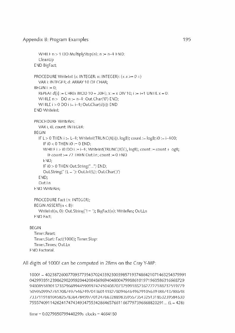
195Appendix B: Program Examples
WHILE n > 1 DO MultiplyStep(n); n := n−1 END;
CleanUp
END BigFact;
PROCEDURE WriteInt (x: INTEGER; n: INTEGER); (* x >= 0 *)
VAR i: INTEGER; d: ARRAY 10 OF CHAR;
BEGIN i := 0;
REPEAT d[i] := CHR(x MOD 10 + 30H); x := x DIV 10; i := i+1 UNTIL x = 0;
WHILE n > i DO n := n−1; Out.Char('0') END;
WHILE i > 0 DO i := i−1; Out.Char(d[i]) END
ENDWriteInt;
PROCEDURE WriteRes;
VAR i, i0, count: INTEGER;
BEGIN
IF L > 0 THEN i := L−1; WriteInt(TRUNC(X[i]), logB); count := logB; i0 := i−100;
IF i0 < 0 THEN i0 := 0 END;
WHILE i > i0 DO i := i−1; WriteInt(TRUNC(X[i]), logB); count := count + logB;
IF count >= 72 THEN Out.Ln; count := 0 END
END;
IF i0 > 0 THEN Out.String("...") END;
Out.String(" (L = "); Out.Int(L); Out.Char(')')
END;
Out.Ln
ENDWriteRes;
PROCEDURE Fact (n: INTEGER);
BEGIN ASSERT(n < B);
WriteInt(n, 0); Out.String("! = "); BigFact(n); WriteRes; Out.Ln
END Fact;
BEGIN
Timer.Reset;
Timer.Start; Fact(1000); Timer.Stop;
Timer.Times; Out.Ln
END Factorial.
All digits of 1000! can be computed in 28ms on the Cray Y_MP:
1000! = 40238726007709377354370243392300398571937486421071463254379991
04299385123986290205920442084869694048004799886101971960586316668729
94808558901323829669944590997424504087073759918823627727188732519779
50595099527612087497546249704360141827809464649629105639388743788648
73371191810458257836478499770124766328898359557354325131853239584630
75557409114262417474349347553428646576611667797396668820291... (L = 428)
time = 0.0279850799440299s clocks = 4664180
![Vector Computers · 2019. 9. 12. · r15 Vector Registers v0 v15 [0] [1] [2] [VLRMAX-1] Vector Length Register VLR v1 Vector Load and Store Instructions VLD v1, r1, r2 Base, r1 Stride,](https://img.pdfslide.us/doc/110x75/6147d90aa830d0442101b391/vector-computers-2019-9-12-r15-vector-registers-v0-v15-0-1-2-vlrmax-1.jpg)