A Primer on Direct Numerical Simulation of Turbulence –Methods, Procedures and Guidelines

Gary N. Coleman and Richard D. Sandberg

Aerodynamics & Flight Mechanics Research GroupSchool of Engineering Sciences, University of Southampton, SO17 1BJ, UK

Technical Report AFM-09/01a (March 2010)

1. INTRODUCTION

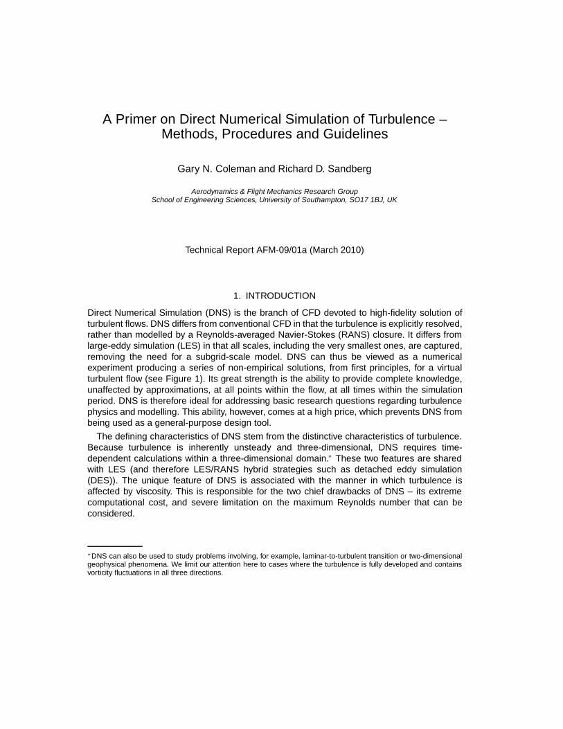
Direct Numerical Simulation (DNS) is the branch of CFD devoted to high-fidelity solution ofturbulent flows. DNS differs from conventional CFD in that the turbulence is explicitly resolved,rather than modelled by a Reynolds-averaged Navier-Stokes (RANS) closure. It differs fromlarge-eddy simulation (LES) in that all scales, including the very smallest ones, are captured,removing the need for a subgrid-scale model. DNS can thus be viewed as a numericalexperiment producing a series of non-empirical solutions, from first principles, for a virtualturbulent flow (see Figure 1). Its great strength is the ability to provide complete knowledge,unaffected by approximations, at all points within the flow, at all times within the simulationperiod. DNS is therefore ideal for addressing basic research questions regarding turbulencephysics and modelling. This ability, however, comes at a high price, which prevents DNS frombeing used as a general-purpose design tool.

The defining characteristics of DNS stem from the distinctive characteristics of turbulence.Because turbulence is inherently unsteady and three-dimensional, DNS requires time-dependent calculations within a three-dimensional domain.∗ These two features are sharedwith LES (and therefore LES/RANS hybrid strategies such as detached eddy simulation(DES)). The unique feature of DNS is associated with the manner in which turbulence isaffected by viscosity. This is responsible for the two chief drawbacks of DNS – its extremecomputational cost, and severe limitation on the maximum Reynolds number that can beconsidered.

∗DNS can also be used to study problems involving, for example, laminar-to-turbulent transition or two-dimensionalgeophysical phenomena. We limit our attention here to cases where the turbulence is fully developed and containsvorticity fluctuations in all three directions.

2 Coleman & Sandberg

Figure 1. Vorticity magnitude contours from spectral Ekman-layer DNS at two Reynolds numbersReE (Spalart et al. 2008). Vertical planes shown are normal to the free-stream velocity, and coverthe same area measured in local boundary-layer thickness. Reynolds number of right-hand-side flow(ReE = 2828) is twice that of left-hand-side flow (ReE = 1414). Courtesy of Dr. R. Johnstone, University

of Southampton.

2. THE REYNOLDS NUMBER CONSTRAINT

Turbulence contains eddies with a wide range of sizes. These eddies interact with eachother in a non-linear fashion through their induced velocity fields, changing the orientationand shape of their neighbours. As first described by Richardson (1922) and quantifiedby Kolmogorov (1941), the net effect of this change-of-shape (i.e. straining) process is to‘cascade’ kinetic energy from the largest to the smallest scales of the turbulence. As a result,the largest eddies are the most energetic, and their size, shape and speed are set by thedetails of the flow configuration, and not directly affected by the viscosity of the fluid. The sizeof the smallest eddies, on the other hand, is determined both by how much energy enters thecascade at the large scales and by the viscosity. The primary role of viscosity is to define thescale at which the energy is dissipated. The Reynolds number of the flow thus determineshow small the smallest scales are, relative to the largest eddies.

This behaviour, known as Reynolds-number similarity,† can be observed in Figure 1, whichpresents DNS results from the same boundary-layer flow at two Reynolds numbers that differby a factor of two. This illustrates the challenge faced by DNS, which must use a domain largeenough to comfortably include the largest naturally-occurring eddies while using a grid fineenough to fully resolve the dissipation scales. Using today’s most capable computers, this canonly be done for Reynolds numbers orders of magnitude smaller than found, for example, infull-scale aeronautical flows.

The manner in which the cost of a DNS scales with Reynolds number can be preciselydetermined for the case of homogeneous isotropic turbulence, for which the size and thespeed of the largest eddies can be characterised by a single length and time scale, �LE andtLE , respectively. Because the largest contribution to the turbulence kinetic energy (per unit

†Reynolds-number similarity is the reason film makers can use small-scale-model special effects, since they yieldturbulent flows whose largest eddies are roughly correct. That these special effects do not look quite right – at leastto the discerning fluid-dynamicist! – compared to the full-scale flow, is a symptom of the truncated range of scales inthe scale-model flow, associated with the vastly different Reynolds numbers.

A PRIMER ON DNS 3

mass) kT = 12q

2 is made by the largest eddies, their characteristic velocity is proportionalto q =

√2kT , and the rate (i.e. flux) of energy eLE leaving the largest eddies scales with

q2/tLE. And since, for this flow, eLE is proportional to ε, the rate at which energy is currentlybeing dissipated at the smallest scales, it is reasonable to assume that tLE goes like q2/ε,and thus (since q ∼ �LE/tLE) that �LE is proportional to q3/ε. Consequently, the intrinsicReynolds number of the turbulence ReT = q�/ν is q4/νε. Following Kolmogorov, assumingthe smallest scales of turbulence are universal and isotropic, and thus depend solely on εand the kinematic viscosity ν, leads on dimensional grounds to definition of the turbulencemicroscale η = (ν3/ε)1/4. The number of grid points N in each direction required for DNSof homogeneous isotropic turbulence will then be of the order �LE/η = (q3/ε)(ε1/4/ν3/4) =(q4/νε)3/4 = Re3/4

T . The total number of grid points, N3 ∼ O[(�LE/η)3], will then scale withRe9/4

T . Factoring in the change in timestep (required for example to maintain the same CFLnumber), the total computational effort isO[Re3T ]. When viewed in terms of operations per gridpoint, the picture becomes slightly worse: if an algorithm requiring N logN operations in eachspatial direction were used (a reasonable estimate for an efficient spectral method), the totaloperational count would be O[Re3

T (34 log ReT )3]. Therefore, doubling the Reynolds number

from a currently attainable value would increase the computational cost (i.e. CPU time,memory) by roughly a factor of 11! Assuming that the current trend of doubling computingpower every 18 months continues and numerical algorithms scale perfectly for even largergrid counts, this implies that for this flow the Reynolds number can be doubled only everyfive to six years. Although the exact Reynolds-number scaling of the cost will vary from flowto flow, and will not always be as stringent as for homogeneous isotropic turbulence,‡ thegeneral point still holds that we are currently far away, and will remain so for the foreseeablefuture, from being able to perform DNS for Reynolds numbers typical of full-scale engineeringand especially geophysical applications.

3. NUMERICAL CONSIDERATIONS

The obligation of having to resolve all spatial and temporal scales of the turbulence requiresthat numerical errors be monitored and controlled. As a result, DNS has historically notused commercial CFD packages, but specially-written codes, optimised for the flow-typesof interest. We now consider the issues that must be addressed by authors and users of DNScodes. The need for DNS algorithms to be efficient – that is, to have a high ratio of accuracyto computational cost – is particularly important.

3.1. Spatial Discretisation

Central to the success of any DNS is the ability to faithfully reproduce all spatial variations ofthe dependent variables. There are a number of strategies that DNS codes have employedto do this, including finite-volume, finite-element, discrete-vortex and B-spline methods.However, for reasons that shall soon be clear, DNS has to this point been dominated by

‡For example, for a boundary-layer simulation only a fraction of the flow will be turbulent and thus adhere to theReynolds-number scaling. An increase in Reynolds number would not affect the resolution in the freestream region.

4 Coleman & Sandberg

spectral and finite-difference schemes. We shall briefly consider each in turn.

3.1.1. Spectral Methods The Reynolds-number constraint and the need to minimisenumerical errors using the available high-performance computing (HPC) resources naturallyled the first practitioners of DNS (e.g. Orszag & Patterson 1972; Kim et al. 1987) to chosespectral methods to account for spatial variations (see Gottlieb & Orszag 1977, Hussaini &Zang 1987, or Canuto et al. 1988 for an overview). Results from a recent spectral DNS areshown in Figure 1. Spectral methods approximate the flow variables as linear combinations(‘expansions’) of global basis functions that involve complex-exponential or orthogonal-polynomial eigensolutions φn(x) (n = 0, 1, 2, . . .) of an appropriate Sturm-Liouville problemover the interval x1 ≤ x ≤ x2. They thus satisfy the orthogonality relationship∫ x2

x1

w(x)φn(x)φm(x)dx = Anδnm, (1)

where An is a positive n-dependent coefficient and δnm is the Kronecker delta (i.e. unitywhen n = m and zero otherwise). The weight function w(x) ≥ 0 defines the resolutioncharacteristics of the basis functions, since in regions where w(x) is largest, φn(x) musthave more zero crossings in order for the weighted product of φn(x) and φm(x) to integrate tozero. The spatial-discretisation procedure will be demonstrated here as if the Navier-Stokesequations L(u) = 0 involve only time t and one spatial direction x, which might be a cartesianor spherical/polar coordinate. ∗ Each dependent variable u(x) is replaced, over the domainx1 ≤ x ≤ x2, by

u(x)← uM (x, t) =M−1∑n=0

αn(t)ψn(x), (2)

where αn are the M expansion coefficients, and, for example, ψn(x) = g(x)φn(x) orh(x)dφn/dx, where g(x) and h(x) might be low-order polynomials that ensure each ψn(x)satisfies the appropriate boundary conditions at x = x1 and x2. When u(x) can be assumedto vary periodically over the distance Λ, it is natural to use a Fourier-series representation,with ψn(x) = φn(x) = exp(iknx), such that

uM (x, t) =+M/2∑

n=−M/2

αn(t) eiknx, (3)

where i =√−1, kn = 2πn/Λ and the weight function w(x) = 1 (indicating uniformly

spaced resolution over Λ = x2 − x1). † For other (wall-bounded) flows, φn(x) might beChebyshev or Jacobi polynomials, which posses w(x) weightings that concentrate resolutioncapability towards the x = x1 and/or x = x2 boundaries, with ψn(x) defined (via g(x) andh(x)) to e.g. automatically satisfy the boundary conditions and (for incompressible flows) thedivergence-free condition (cf. Spalart et al. 1991).

∗The generalisation to three dimensions is straightforward, involving expansions of expansion coefficients.†Since αM/2 = α−M/2 (Press et al. 1986), equation (3) is shown with M + 1, rather than M , coefficients, in orderto make explicit for later use that the magnitude of the maximum wavenumber kmax = |kM/2| = π

/(Λ/M).

A PRIMER ON DNS 5

Replacing u(x) with uM (x) in L(u) = 0, introduces the nonzero residual RM = L(uM ). Tominimise the error, the product of the residual and each of the basis functions is set to zero,such that ∫ x2

x1

w(x)ψ�mRMdx = 0 for m = 0, 1, 2, . . .M − 1, (4)

where ψ�m is the complex-conjugate of ψm(x). The result is the semi-discrete M × M

system of coupled first-order ordinary differential equations in the dependent variable �α(t) =[α0(t), α1(t), . . . , αM−1(t)]T , with

Ad�αdt

= B�α+ �f, (5)

and where A and B are narrow-banded M × M matrices, ‡ whose elements (which areindependent of time) are defined by (1) and w(x). The quantity �f in (5) accounts for thenonlinear (e.g. convection) terms in L. To improve efficiency, these are evaluated usinga collocation/pseudo-spectral approximation (Gottlieb & Orszag 1977). The process ofevaluating the nonlinear terms in this manner opens the calculation to errors introduced bythe numerical quadrature. Since they consist of products of expansions in φn up to order M ,the nonlinear terms will effectively involve an expansion up to order 2M . Consequently, if thenumber of collocation points N within x1 ≤ x ≤ x2 is not larger than the number of expansioncoefficients M , the quadrature will not be exact, leading to aliasing errors.§ The algorithm iscompleted by applying a time-marching scheme to (5), to yield �α(t) and therefore uM (x, t) atdiscrete times (see section 3.2).

Spectral methods have a number of significant advantages. Chief among these is thefact that when the basis-function variations correctly ‘fit’ the dependent-variable variations(in terms of smoothness, boundary conditions, and regions of most rapid spatial change)the magnitude of the expansion coefficients αn goes to zero as M → ∞, and do so suchthat the error decreases faster than any power of 1/M (Gottlieb & Orszag 1977). Therefore,in contrast to a pth-order finite-difference approximation, whose error is proportional to(Δx)p ∝ (1/M)p, a spectral method converges with exponential or ‘infinite-order’ accuracy.The spatial accuracy of spectral DNS can thus be easily determined by confirming that themagnitude of the expansion coefficients |αn| → 0 as n→M , which provides a quality-controlcheck that is only available to non-spectral methods via a grid-refinement study. The qualityof the domain size can also be deduced from the low-n variation of αn. Another attractivefeature of Fourier- and Chebyshev-based methods is the ability to employ fast transformswhen computing uM from αn, and when using the collocation/pseudo-spectral procedure tocalculate �f in (5), both of which must be done at each time step.

‡The banded nature of A and B allows the time advancement to be effected quite efficiently. When the basisfunctions are built from orthogonal polynomials (e.g. Chebyshev or Jacobi), the matrix inversion involved in solving(5) is often able to use the Thomas algorithm for a tri- or penta-diagonal system. When the basis functions arecomplex exponentials, A and B are diagonal, the Fourier coefficients are completely decoupled, and the time-advance procedure is trivial.§For incompressible flows, aliasing errors will be avoided if N ≥ 3M/2 (Spalart et al. 1991). For compressible-flowDNS, for which the Navier-Stokes equations involve triple products of dependent variables, a straightforward remedyis not available, and the only recourse is to make N/M as large as possible. Some incompressible-flow algorithms(e.g. Kim et al. 1987) are also not able to remove aliasing errors in all directions, because e.g. they use linearcombinations of the M expansion coefficients to enforce the no-slip boundary conditions.

6 Coleman & Sandberg

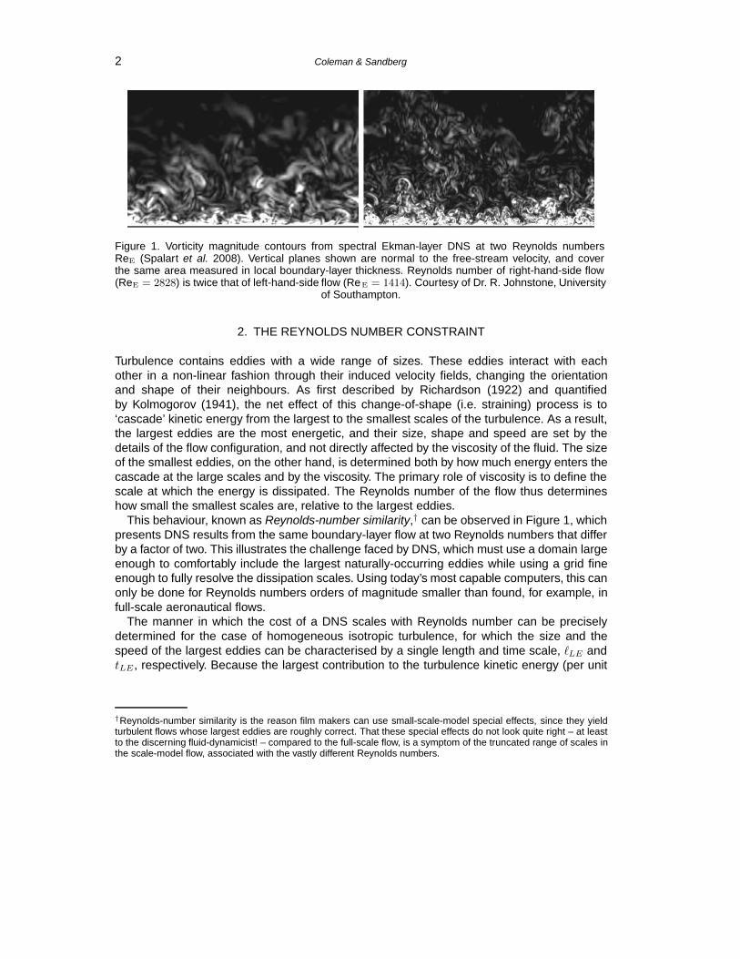
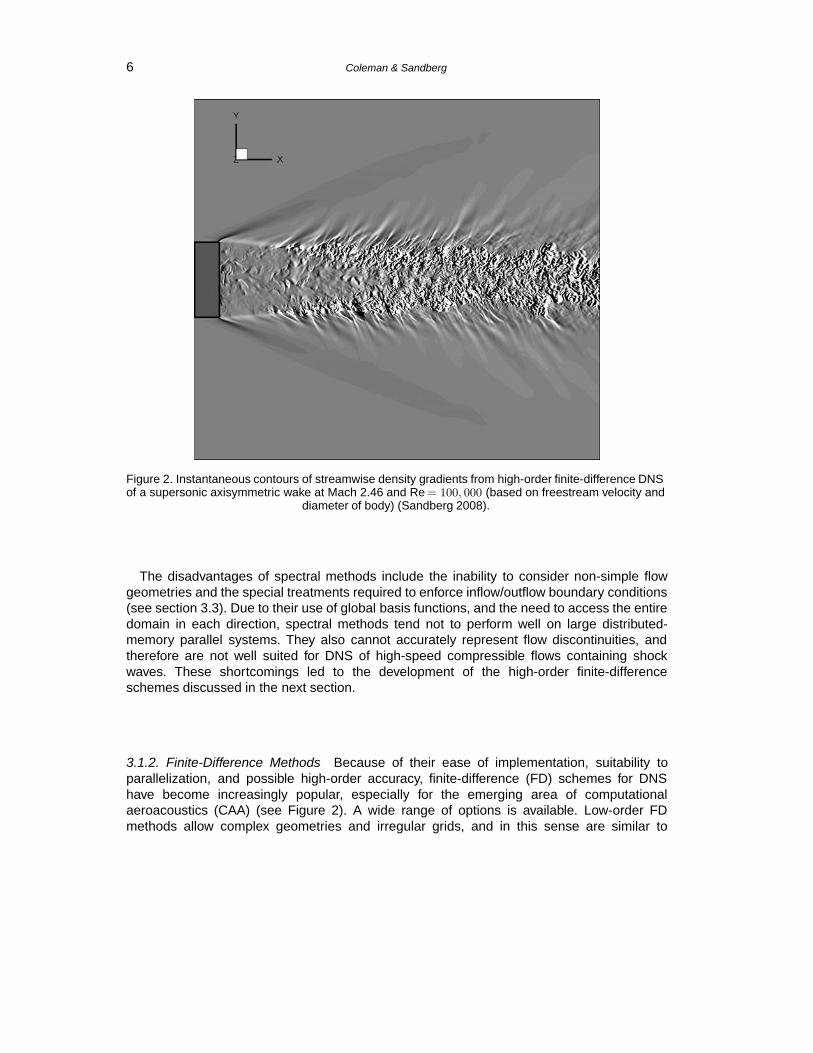
Figure 2. Instantaneous contours of streamwise density gradients from high-order finite-difference DNSof a supersonic axisymmetric wake at Mach 2.46 and Re = 100, 000 (based on freestream velocity and

diameter of body) (Sandberg 2008).

The disadvantages of spectral methods include the inability to consider non-simple flowgeometries and the special treatments required to enforce inflow/outflow boundary conditions(see section 3.3). Due to their use of global basis functions, and the need to access the entiredomain in each direction, spectral methods tend not to perform well on large distributed-memory parallel systems. They also cannot accurately represent flow discontinuities, andtherefore are not well suited for DNS of high-speed compressible flows containing shockwaves. These shortcomings led to the development of the high-order finite-differenceschemes discussed in the next section.

3.1.2. Finite-Difference Methods Because of their ease of implementation, suitability toparallelization, and possible high-order accuracy, finite-difference (FD) schemes for DNShave become increasingly popular, especially for the emerging area of computationalaeroacoustics (CAA) (see Figure 2). A wide range of options is available. Low-order FDmethods allow complex geometries and irregular grids, and in this sense are similar to

A PRIMER ON DNS 7

finite-volume methods.¶ The computational efficiency of low-order (especially upwind) FDapproximations (FDA) is often unacceptable, requiring many more grid points than a spectralmethod to achieve the same accuracy. This can be demonstrated by applying a low-order FDAon a uniform grid with constant spacing Δx = Λ/N for j = 0, 1, . . .N to a periodic function

u(x) =+kmax∑

k=−kmax

u(k)eikxj , (6)

where kmax = π/Δx (see (3)) is taken to be large enough to capture all spatial variations inu(x). At xj = jΔx, the function is given by uj = u(xj) =

∑k u(k) eikxj (the implicit ±kmax

limits on the k summation will hereinafter be suppressed). We consider the accuracy of theone-sided backward-difference approximation at xj ,

ΔuΔx

∣∣∣∣xj

=uj − uj−1

Δx, (7)

by applying it to the periodic function at xj , resulting in

ΔuΔx

∣∣∣∣xj

=∑

k

1Δx

[1− e−ikΔx

]u(k) eikxj . (8)

By analogy to the exact result, du/dx =∑

k iku(k) eikx, equation (8) can be written

ΔuΔx

∣∣∣∣xj

=∑

k

ik′u(k)eikxj , (9)

where k′ is the modified wavenumber , which for this one-sided FDA is

k′(k) = sin(kΔx)/Δx+ i[cos(kΔx)− 1]/Δx. (10)

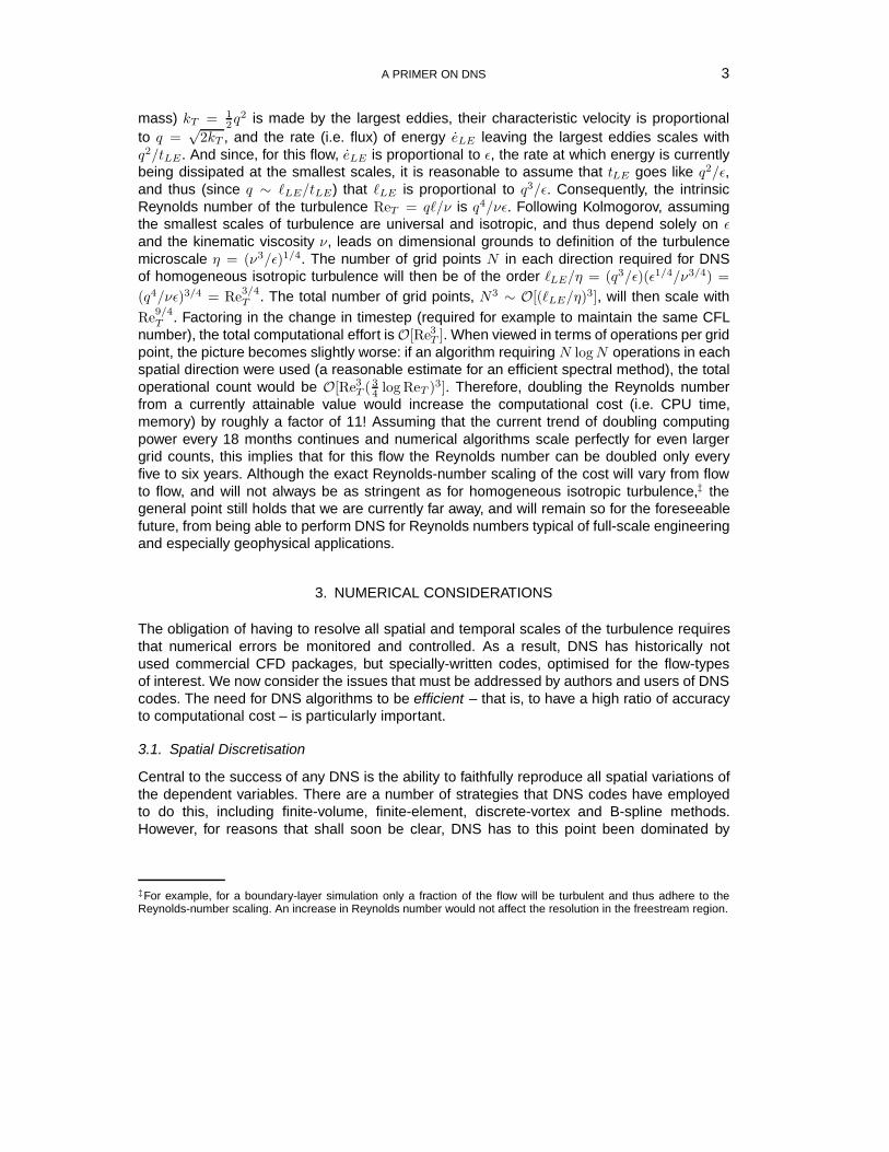
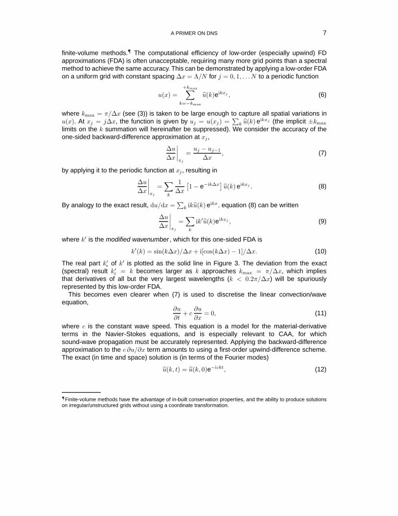
The real part k′r of k′ is plotted as the solid line in Figure 3. The deviation from the exact(spectral) result k′r = k becomes larger as k approaches kmax = π/Δx, which impliesthat derivatives of all but the very largest wavelengths (k < 0.2π/Δx) will be spuriouslyrepresented by this low-order FDA.

This becomes even clearer when (7) is used to discretise the linear convection/waveequation,

∂u

∂t+ c

∂u

∂x= 0, (11)

where c is the constant wave speed. This equation is a model for the material-derivativeterms in the Navier-Stokes equations, and is especially relevant to CAA, for whichsound-wave propagation must be accurately represented. Applying the backward-differenceapproximation to the c ∂u/∂x term amounts to using a first-order upwind-difference scheme.The exact (in time and space) solution is (in terms of the Fourier modes)

u(k, t) = u(k, 0)e−ickt, (12)

¶Finite-volume methods have the advantage of in-built conservation properties, and the ability to produce solutionson irregular/unstructured grids without using a coordinate transformation.

8 Coleman & Sandberg

0 0.5 10

0.5

1

k/kmax

k′ r/km

ax

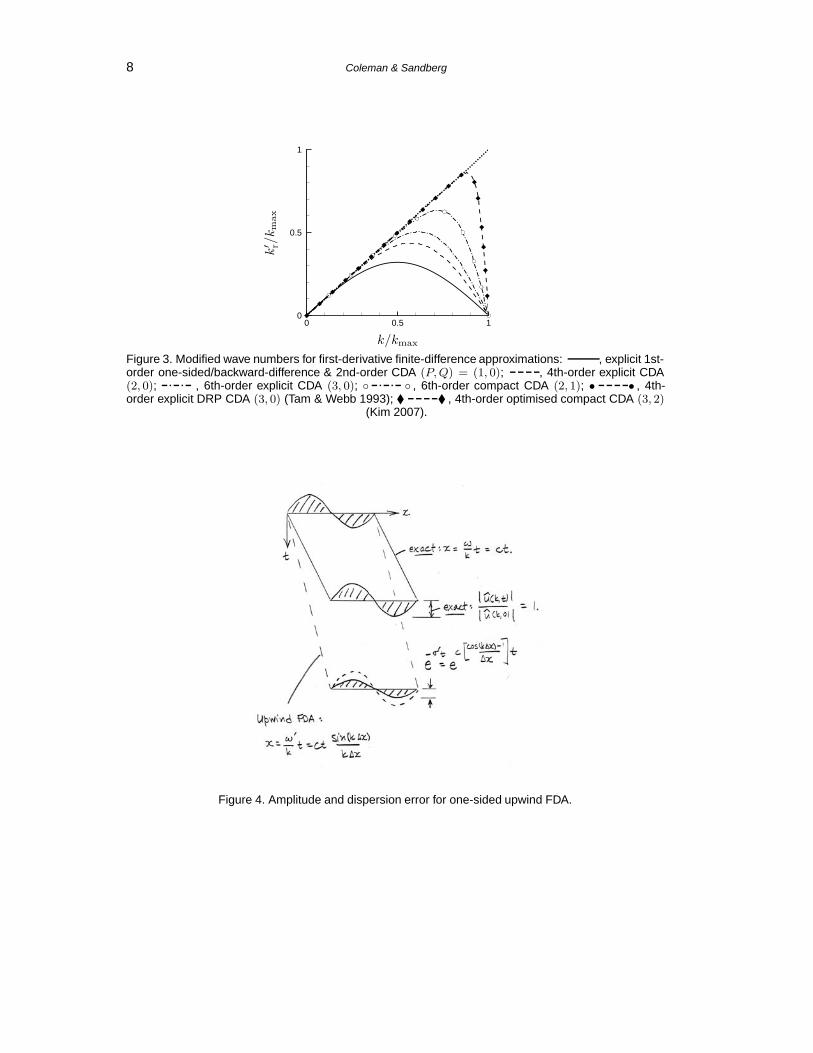
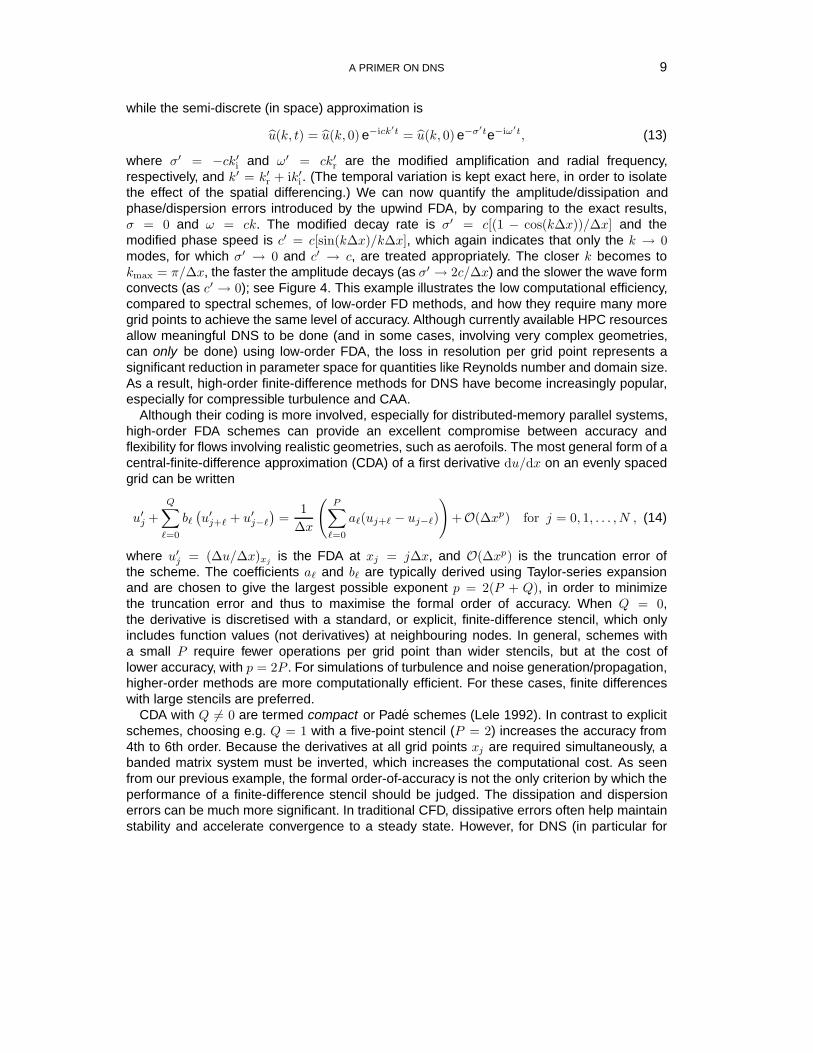
Figure 3. Modified wave numbers for first-derivative finite-difference approximations: , explicit 1st-order one-sided/backward-difference & 2nd-order CDA (P, Q) = (1, 0); , 4th-order explicit CDA(2, 0); , 6th-order explicit CDA (3, 0); ◦ ◦ , 6th-order compact CDA (2, 1); • • , 4th-order explicit DRP CDA (3, 0) (Tam & Webb 1993); � � , 4th-order optimised compact CDA (3, 2)

(Kim 2007).

Figure 4. Amplitude and dispersion error for one-sided upwind FDA.

A PRIMER ON DNS 9

while the semi-discrete (in space) approximation is

u(k, t) = u(k, 0) e−ick′t = u(k, 0) e−σ′te−iω′t, (13)

where σ′ = −ck′i and ω′ = ck′r are the modified amplification and radial frequency,respectively, and k′ = k′r + ik′i . (The temporal variation is kept exact here, in order to isolatethe effect of the spatial differencing.) We can now quantify the amplitude/dissipation andphase/dispersion errors introduced by the upwind FDA, by comparing to the exact results,σ = 0 and ω = ck. The modified decay rate is σ′ = c[(1 − cos(kΔx))/Δx] and themodified phase speed is c′ = c[sin(kΔx)/kΔx], which again indicates that only the k → 0modes, for which σ′ → 0 and c′ → c, are treated appropriately. The closer k becomes tokmax = π/Δx, the faster the amplitude decays (as σ′ → 2c/Δx) and the slower the wave formconvects (as c′ → 0); see Figure 4. This example illustrates the low computational efficiency,compared to spectral schemes, of low-order FD methods, and how they require many moregrid points to achieve the same level of accuracy. Although currently available HPC resourcesallow meaningful DNS to be done (and in some cases, involving very complex geometries,can only be done) using low-order FDA, the loss in resolution per grid point represents asignificant reduction in parameter space for quantities like Reynolds number and domain size.As a result, high-order finite-difference methods for DNS have become increasingly popular,especially for compressible turbulence and CAA.

Although their coding is more involved, especially for distributed-memory parallel systems,high-order FDA schemes can provide an excellent compromise between accuracy andflexibility for flows involving realistic geometries, such as aerofoils. The most general form of acentral-finite-difference approximation (CDA) of a first derivative du/dx on an evenly spacedgrid can be written

u′j +Q∑

�=0

b�(u′j+� + u′j−�

)=

1Δx

(P∑

�=0

a�(uj+� − uj−�)

)+O(Δxp) for j = 0, 1, . . . , N , (14)

where u′j = (Δu/Δx)xj is the FDA at xj = jΔx, and O(Δxp) is the truncation error ofthe scheme. The coefficients a� and b� are typically derived using Taylor-series expansionand are chosen to give the largest possible exponent p = 2(P + Q), in order to minimizethe truncation error and thus to maximise the formal order of accuracy. When Q = 0,the derivative is discretised with a standard, or explicit, finite-difference stencil, which onlyincludes function values (not derivatives) at neighbouring nodes. In general, schemes witha small P require fewer operations per grid point than wider stencils, but at the cost oflower accuracy, with p = 2P . For simulations of turbulence and noise generation/propagation,higher-order methods are more computationally efficient. For these cases, finite differenceswith large stencils are preferred.

CDA with Q = 0 are termed compact or Pade schemes (Lele 1992). In contrast to explicitschemes, choosing e.g. Q = 1 with a five-point stencil (P = 2) increases the accuracy from4th to 6th order. Because the derivatives at all grid points xj are required simultaneously, abanded matrix system must be inverted, which increases the computational cost. As seenfrom our previous example, the formal order-of-accuracy is not the only criterion by which theperformance of a finite-difference stencil should be judged. The dissipation and dispersionerrors can be much more significant. In traditional CFD, dissipative errors often help maintainstability and accelerate convergence to a steady state. However, for DNS (in particular for

10 Coleman & Sandberg

compressible turbulence and especially CAA applications), dissipation must be minimisedto avoid, for example, attenuation of acoustic waves that propagate over long distances.‖

Dispersion errors are also of crucial importance, because of their potential for introducingunphysical behaviour in the acoustic field (for CAA) or the evolution of the vortical structure ofthe turbulence.

We have already seen, for the first-order upwind scheme discussed earlier, how dissipationand dispersion errors are determined by the modified wavenumber profile k′(k) of the FDAin question, and the transport equation that the FDA is used to discretise. The modifiedwavenumber for an arbitrary first-derivative CDA scheme can be determined by substitutingu′j =

∑k ik′u(k) eikxj into (14), and using the trigonometric relations eiθ + e−iθ = 2 cos θ and

eiθ − e−iθ = 2i sin θ, to find

k′ =

(1

Δx

)∑P�=0 2a� sin(�kΔx)

1 +∑Q

�=0 2b� cos(�kΔx). (15)

Note that since it has no imaginary component, ∗∗ k′ will introduce no dissipation/amplitudeerror when applied to the convective term of the linear wave equation (11); significantdispersion errors, however, are possible, since the modified frequency ω′ = ck′(k) associatedwith (15) approaches zero as kΔx→ π.

The modified wavenumbers for several CDA schemes, both explicit and compact, areincluded in Figure 3. Although the 2nd-order CDA does not spuriously introduce an imaginarywavenumber, its real component k′r(k) is (and therefore its wave-equation dispersioncharacteristics are) identical to that of the first-order FDA considered above (solid line inFigure 3). Increasing the width of the stencil has a noticeable positive effect on the resolutionof the explicit schemes, as evidenced by the upward shift of the maximum k′ as the orderincreases, from 2nd to 4th to 6th. Note that a compact scheme with the same formal orderof accuracy performs significantly better in terms of wavenumber resolution characteristics,albeit at a higher computational cost (compare the dash-dot curves with and without opensymbols).

Given that the formal order of accuracy is not necessarily the most important feature of aFD scheme, it is logical to use the coefficients a� and b� in (14) to optimise the wavenumberresolution characteristics, rather than minimise the truncation error. Noteworthy examplesof this exercise are shown in Figure 3, which involve sacrificing formal order of accuracyin order to push the maximum k′ towards the exact kmax = π/Δx limit. This can be donefor both explicit (Q = 0) and compact (Q ≥ 1) schemes. An example of both is shown inFigure 3 (solid symbols). The optimised k′(k) profile for the 4th-order compact scheme isparticularly impressive. Because an increase in maximum k′ allows a grid to be coarsenedby the same factor to resolve the same flow features, these modified schemes represent asignificant increase in computational efficiency, compared to a standard/explicit CDA usingthe same resolution, which can outweigh the additional cost of the more complex algorithm.

The discussion so far has been restricted to central interior schemes on uniform grids.FDA are also needed for the boundaries. Typically, boundary stencils are one-sided, so

‖Minimising dissipation is crucial for CAA, since the energy of the acoustic field is typically orders of magnitudesmaller, and occurs at much different wavelengths, than that of the hydrodynamic field.∗∗A property unique to central-difference schemes on uniform grids.

A PRIMER ON DNS 11

maintaining good wavenumber resolution characteristics is difficult (see Kim 2007 for adiscussion of available options). Furthermore, finite-difference methods require generalcurvilinear coordinates when they are applied to complex geometries. This introduces metricterms to map from (a uniformly spaced grid in) computational space to physical space. Gridstretching is also routinely used, in particular for wall-bounded flows and/or for aeroacousticproblems where the acoustic wavelength is much larger than the hydrodynamic scales inthe turbulent source region, which permits considerable coarsening of the grid towards thefar field. The above Fourier-based modified wavenumber analysis cannot be directly appliedto these cases, since the grid metrics introduce non-constant coefficients in the governingequations. For more details and analysis of the wavenumber resolution characteristics onnon-uniform and curvilinear meshes, the reader is referred to Colonius & Lele (2004).

3.2. Temporal Discretisation

Two general methods of time discretisation can be distinguished: (i) explicit methods, whereall spatial derivatives needed to advance the solution in time are evaluated at earlier timesteps; (ii) implicit schemes, where the spatial derivatives are approximated using informationat the new time step. In addition, a combination of the two approaches have been used forreasons that will become apparent soon, with, for example, an explicit method applied tothe convective terms and an implicit method to the viscous terms. Whichever time-marchingscheme is chosen, it needs to be both accurate (i.e. possess good frequency resolutioncharacteristics, similar to the wavenumber equivalent for spatial schemes) and stable.

Accuracy of the temporal discretisation is paramount because the wide range of lengthscales found in turbulence is associated with a similarly wide range of timescales. In analogyto the length scales from section 2, the time scales of the largest and smallest eddies tLE

and tη are respectively proportional to q2/ε and (ν/ε)1/2 (Kolmogorov 1941). The turbulenceReynolds number ReT = q4/νε is therefore proportional to (tLE/tη)2 which demonstratesthat the Reynolds-number constraint previously discussed also applies to the time-integrationof the Navier–Stokes equations. A system of differential equations yielding solutions withhighly disparate time scales is termed numerically stiff.∗ When dealing with stiff systems,both accuracy and stability considerations require that the product of the timestep and thelargest eigenvalue of the semi-discrete system produced by the spatial discretisation must bekept below a certain threshold. This threshold depends on the details of both the spatial andtime-marching scheme used.

Accuracy and stability are tightly connected, making it impossible to treat either requirementindividually. Generally, explicit time-integration schemes can be devised with p-th order ofaccuracy, and similar to optimization of spatial FD schemes for improved wavenumberaccuracy, time-advancement schemes can also be optimized for frequency resolution ratherthan the highest possible order of accuracy. However, as will be shown with an examplebelow, the allowable timesteps for explicit methods must be below a certain value to ensurenumerical stability. It is often the case that the maximum permitted timestep is well belowthe accuracy threshold required to resolve all physical turbulence scales. For these flows,

∗Formally, numerically stiff systems are those whose largest and smallest eigenvalues of the discretised system havevery different magnitudes.

12 Coleman & Sandberg

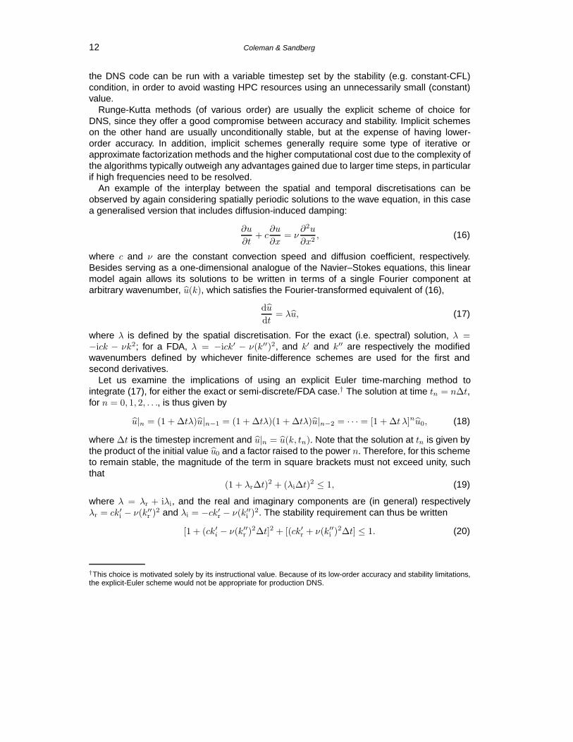
the DNS code can be run with a variable timestep set by the stability (e.g. constant-CFL)condition, in order to avoid wasting HPC resources using an unnecessarily small (constant)value.

Runge-Kutta methods (of various order) are usually the explicit scheme of choice forDNS, since they offer a good compromise between accuracy and stability. Implicit schemeson the other hand are usually unconditionally stable, but at the expense of having lower-order accuracy. In addition, implicit schemes generally require some type of iterative orapproximate factorization methods and the higher computational cost due to the complexity ofthe algorithms typically outweigh any advantages gained due to larger time steps, in particularif high frequencies need to be resolved.

An example of the interplay between the spatial and temporal discretisations can beobserved by again considering spatially periodic solutions to the wave equation, in this casea generalised version that includes diffusion-induced damping:

∂u

∂t+ c

∂u

∂x= ν

∂2u

∂x2, (16)

where c and ν are the constant convection speed and diffusion coefficient, respectively.Besides serving as a one-dimensional analogue of the Navier–Stokes equations, this linearmodel again allows its solutions to be written in terms of a single Fourier component atarbitrary wavenumber, u(k), which satisfies the Fourier-transformed equivalent of (16),

dudt

= λu, (17)

where λ is defined by the spatial discretisation. For the exact (i.e. spectral) solution, λ =−ick − νk2; for a FDA, λ = −ick′ − ν(k′′)2, and k′ and k′′ are respectively the modifiedwavenumbers defined by whichever finite-difference schemes are used for the first andsecond derivatives.

Let us examine the implications of using an explicit Euler time-marching method tointegrate (17), for either the exact or semi-discrete/FDA case.† The solution at time tn = nΔt,for n = 0, 1, 2, . . ., is thus given by

u|n = (1 + Δtλ)u|n−1 = (1 + Δtλ)(1 + Δtλ)u|n−2 = · · · = [1 + Δt λ]nu0, (18)

where Δt is the timestep increment and u|n = u(k, tn). Note that the solution at tn is given bythe product of the initial value u0 and a factor raised to the power n. Therefore, for this schemeto remain stable, the magnitude of the term in square brackets must not exceed unity, suchthat

(1 + λrΔt)2 + (λiΔt)2 ≤ 1, (19)

where λ = λr + iλi, and the real and imaginary components are (in general) respectivelyλr = ck′i − ν(k′′r )2 and λi = −ck′r − ν(k′′i )2. The stability requirement can thus be written

[1 + (ck′i − ν(k′′r )2Δt]2 + [(ck′r + ν(k′′i )2Δt] ≤ 1. (20)

†This choice is motivated solely by its instructional value. Because of its low-order accuracy and stability limitations,the explicit-Euler scheme would not be appropriate for production DNS.

A PRIMER ON DNS 13

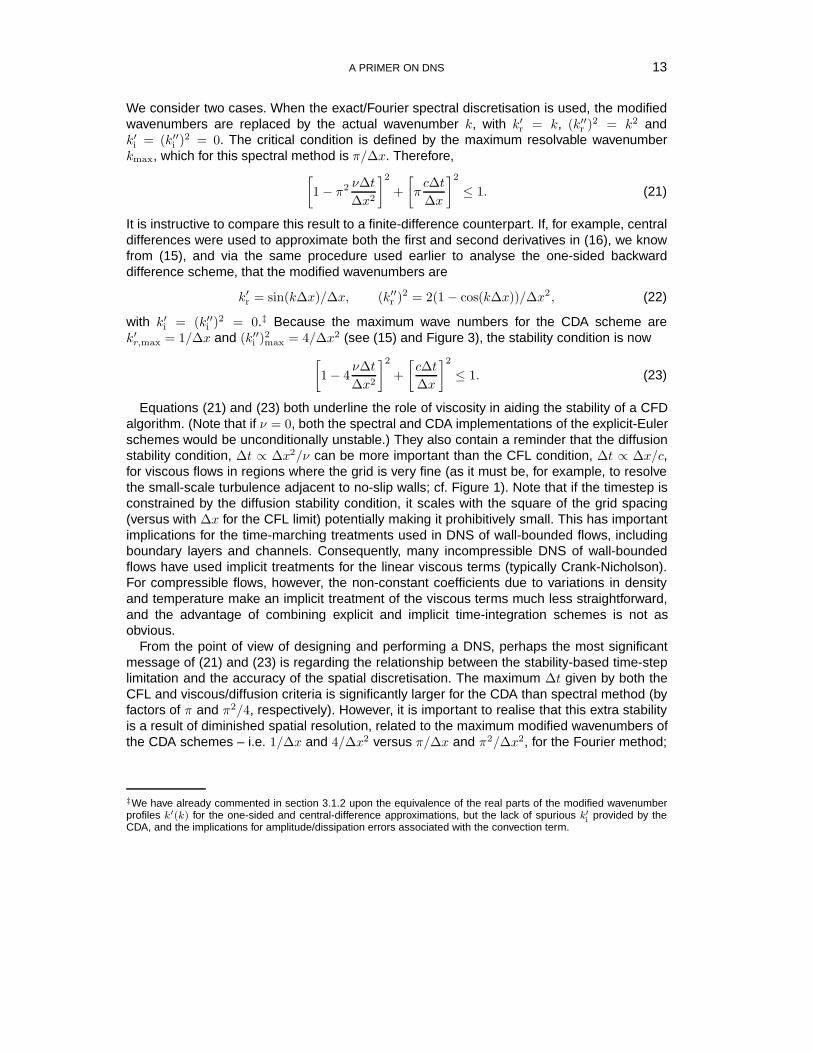
We consider two cases. When the exact/Fourier spectral discretisation is used, the modifiedwavenumbers are replaced by the actual wavenumber k, with k′r = k, (k′′r )2 = k2 andk′i = (k′′i )2 = 0. The critical condition is defined by the maximum resolvable wavenumberkmax, which for this spectral method is π/Δx. Therefore,[

1− π2 νΔtΔx2

]2+[πcΔtΔx

]2≤ 1. (21)

It is instructive to compare this result to a finite-difference counterpart. If, for example, centraldifferences were used to approximate both the first and second derivatives in (16), we knowfrom (15), and via the same procedure used earlier to analyse the one-sided backwarddifference scheme, that the modified wavenumbers are

k′r = sin(kΔx)/Δx, (k′′r )2 = 2(1− cos(kΔx))/Δx2, (22)

with k′i = (k′′i )2 = 0.‡ Because the maximum wave numbers for the CDA scheme arek′r,max = 1/Δx and (k′′i )2max = 4/Δx2 (see (15) and Figure 3), the stability condition is now[

1− 4νΔtΔx2

]2+[cΔtΔx

]2≤ 1. (23)

Equations (21) and (23) both underline the role of viscosity in aiding the stability of a CFDalgorithm. (Note that if ν = 0, both the spectral and CDA implementations of the explicit-Eulerschemes would be unconditionally unstable.) They also contain a reminder that the diffusionstability condition, Δt ∝ Δx2/ν can be more important than the CFL condition, Δt ∝ Δx/c,for viscous flows in regions where the grid is very fine (as it must be, for example, to resolvethe small-scale turbulence adjacent to no-slip walls; cf. Figure 1). Note that if the timestep isconstrained by the diffusion stability condition, it scales with the square of the grid spacing(versus with Δx for the CFL limit) potentially making it prohibitively small. This has importantimplications for the time-marching treatments used in DNS of wall-bounded flows, includingboundary layers and channels. Consequently, many incompressible DNS of wall-boundedflows have used implicit treatments for the linear viscous terms (typically Crank-Nicholson).For compressible flows, however, the non-constant coefficients due to variations in densityand temperature make an implicit treatment of the viscous terms much less straightforward,and the advantage of combining explicit and implicit time-integration schemes is not asobvious.

From the point of view of designing and performing a DNS, perhaps the most significantmessage of (21) and (23) is regarding the relationship between the stability-based time-steplimitation and the accuracy of the spatial discretisation. The maximum Δt given by both theCFL and viscous/diffusion criteria is significantly larger for the CDA than spectral method (byfactors of π and π2/4, respectively). However, it is important to realise that this extra stabilityis a result of diminished spatial resolution, related to the maximum modified wavenumbers ofthe CDA schemes – i.e. 1/Δx and 4/Δx2 versus π/Δx and π2/Δx2, for the Fourier method;

‡We have already commented in section 3.1.2 upon the equivalence of the real parts of the modified wavenumberprofiles k′(k) for the one-sided and central-difference approximations, but the lack of spurious k′i provided by theCDA, and the implications for amplitude/dissipation errors associated with the convection term.

14 Coleman & Sandberg

see (22). In other words, the FD algorithm is able to take larger times steps because it is notfaithfully representing the k → kmax wavenumbers. One should be aware of the potential fora spatial scheme to unphysically enhance a DNS code’s stability characteristics.

The stability criteria obtained from one-dimensional linear model problems usually providea reliable estimate of what is required in practice for nonlinear and multi-dimensionalsimulations. In many cases however, in particular when applying optimized methods andhigh-order-accurate schemes, spurious oscillations in the high wavenumber range can occur.In addition to insufficient grid resolution, several factors can cause this undesired behaviour.First, a mismatch between interior and boundary FD schemes can make the overall algorithmunstable. This is in particular true for compact FD schemes combined with non-compactboundary schemes. To ensure stability of the entire scheme, a stability analysis needsto be performed of the overall method and not just the scheme used for the interiorderivatives. Second, nonlinearities can cause a method that was stable for a linear equationto be unstable. Several approaches have been proposed to treat the nonlinear terms toensure long-time stability, such as entropy splitting (Sandham et al. 2002), higher-entropyconservation (Honein & Moin 2004), skew-symmetric splitting (Kennedy & Gruber 2008), orexplicit filtering (Visbal & Gaitonde 2001).

3.3. Boundary & Initial Conditions

The unsteady three-dimensional nature of turbulence leads to some special problems whenit comes to defining and enforcing appropriate boundary conditions for DNS. Given that themost appropriate boundary conditions are Navier-Stokes solutions, the problem is especiallychallenging for spatially developing flows, such as boundary layers, that are fully turbulent atthe inflow boundary of the domain, since these require complete, physically realistic, turbulenthistories for each of the dependent variables to be prescribed at each point on the inflowplane. (Flows for which the turbulence does not convect across the domain boundaries canhave other boundary-condition complications; see below.) One of the most attractive featuresof Fourier spectral methods is their ability to sidestep this problem: applying them in directionsin which the turbulence is statistically homogeneous, for which it is natural to assume spatialperiodicity (provided the domain is large enough), automatically produces conditions whosehistory and spatial structure fully satisfy the governing equations. This is true both when thehomogeneous direction does and does not coincide with the direction of the net mean flow (forexample, in both the longitudinal and lateral directions of plane-channel/Poiseuille or Couetteflow). As a result, the early (Fourier/spectral) DNS work focused on parallel flows, the first ofwhich where statistically stationary (e.g. fully developed plane-channel flow) and realisablein the laboratory. Later, the parallel-flow geometry was used for DNS of time-developinganalogues of spatially developing cases (boundary layers, plane mixing layers, wakes, etc).For these time-developing flows, the task of defining a sequence of physical turbulent inflowconditions is replaced by specifying a single turbulent-field initial condition (revealing anotheradvantage of using the time-developing parallel-flow analogue).

There are a number of strategies currently available for generating the required turbulentinflow conditions for non-parallel flows. Fourier schemes can be altered to accommodatespatial flows by adding non-physical terms to the governing equations that are active onlyin fringe or sponge regions at the downstream end of the periodic domain. These termsartificially ‘process’ the turbulence so that it ‘forgets’ the outflow state, and re-enters the

A PRIMER ON DNS 15

upstream domain suited to the local flow conditions (see Spalart & Watmuff 1993 for details).§

However, for the many flows for which Fourier methods are not viable (due for example tocomplex geometries or rapid streamwise variations), other discretisation approaches, such asfinite-difference or finite-volume methods, must be used, and the inflow boundary conditionsmust be explicitly specified. One option is to let the flow transition to turbulence within theflow domain, by specifying a relevant base flow at the inlet (e.g. a laminar profile) superposedwith suitable perturbations (either low-amplitude disturbances that feed linear instabilities,or larger-amplitude fluctuations tuned to efficiently trigger nonlinear bypass transition.¶) Allof these approaches involve sacrificing a fraction of the domain to allow the turbulence toreach the desired fully physical state. In contrast, one can use a companion/precursor DNSto obtain the turbulent inflow data, or employ a self-contained ‘recycling’ technique, wherebyturbulent results from within the domain are extracted, rescaled and specified at the inflowplane at each time step (Lund et al. 1998). Each of these approaches represents differentcompromises between minimising, on the one hand, the non-physical region of the domainused to achieve a fully developed state, and, on the other, the computational cost.

Outflow and far-field boundary conditions can also require some care, especially forexternal flows. (There is usually no ambiguity about the boundary conditions for internal, wall-bounded/duct flows, which typically involve a combination of no-slip or transpiration conditionsat walls, and zero-derivative or periodic conditions at outflows.‖) For most external flows, theactual physical domain will be much larger than the largest affordable computational domain.The challenge is to devise boundary conditions that allow for flow disturbances (vorticity,acoustic or entropy waves) to cross the finite/truncated-domain boundaries without generatingexcessive spurious waves that are reflected back to the region of interest. The quality ofDNS for CAA in particular is tied to an ability to meet this requirement. Various so-callednon-reflecting boundary conditions have been derived using characteristics-based boundaryconditions (Thompson 1987). In applications where these boundary conditions are unable tosufficiently attenuate spurious reflections, additional fringe/sponge layers, involving filtering,grid-stretching, additional convection terms, or combinations thereof, can be employed.

The quality of the initial conditions needed by a DNS varies widely. For stationary flows,the only benefit of specifying a fully physical turbulent initial condition is to minimise the timeit takes to overcome an initial transient; because the long-time flow statistics do not dependon the initial condition, totally unphysical conditions (e.g. random velocity fluctuations) can bespecified. ∗∗

§In addition to representing spatially developing flows, Fourier schemes can also be adapted to exactly represent acompact region of turbulence in an unbounded/infinite domain (see Corral & Jim‘enez 1995).¶These larger-amplitude disturbances could be, for example, based on a synthetic/analytic time-dependent modelof near-wall turbulence structures (Sandham et al. 2003), or the result of applying digital filters to unsteady randomperturbations in order to impose the desired length- and time-scales at the inflow (Xie & Castro 2008).‖Very complex surface geometries, such as roughness elements, can be approximated using immersed boundarymethods (Goldstein et al. 1993).∗∗A key requirement is to determine when the flow reaches the beginning of its statistically steady state, after whichtime-averaging of data should begin. This can be achieved by monitoring higher-order statistics and histories ofglobal quantities, such as plane-averaged shear stress, bulk mass flux, or integrated turbulence kinetic energy. Toavoid unnecessary computational cost, it is usually wise to accelerate the arrival of the stationary state by beginningthe simulation on a spatial grid that is significantly coarser than that required to resolve the flow in question. Thiscould be done in a number of steps, increasing the resolution after the under-resolved flow has equilibrated, as

16 Coleman & Sandberg

For flows where it is important to impose physical fully turbulent initial conditions (such asthe parallel-flow time-developing analogues of spatial flows mentioned earlier; cf. Colemanet al. 2003), they can be obtained using counterparts of the turbulence inflow generationstrategies (except the recycling techniques) mentioned above.

3.4. Code Validation & Resolution Guidelines

The fundamental requirement of any DNS is to produce results that can be trusted.Consequently, especially in light of the computational costs involved, it is essential that everyDNS code must be properly validated before it enters ‘production’ and then used appropriatelythereafter. In this section (adapted from the recommendations given by Sandham (2005)) weoffer suggestions about how this might be done.

• A newly developed or modified code must be able to reproduce analytic solutions andasymptotic limits. For example, laminar channel, pipe or boundary-layer flows can becomputed and compared to the exact results. A more challenging (and therefore morevaluable) test is prediction of growth rates and phase speeds of small disturbances in anappropriate background flow. For fully turbulent cases, rapid-distortion theory (for whichonly the linear terms in the governing equations are active) often provides a usefulbenchmark, in terms of closed-form predictions of histories of turbulence statistics.Another powerful method, whose utility does not seem to have been fully appreciated, isto prescribe analytic unsteady, three-dimensional test functions∗ for all variables, and tomodify the governing equations so that they are exactly satisfied by these test functions.This involves adding forcing terms† that cause the left- and right-hand sides to formallyagree. The difference between the code results and the test functions, at each point inthe domain at each time, can then be monitored, and quantified in terms of the sizes ofthe grid spacing and time step.

• When assessing the sufficiency of the spatial and temporal resolution for DNS,one cannot follow the standard CFD practice of demonstrating grid and time-stepindependence by converging towards the same point-wise solution history usingdifferent grids and different time-step sizes. This is because of the well-knowncharacteristic of turbulence (often referred to as extreme sensitivity to initial conditions)that small differences between two realisations of turbulence quickly lead to divergenceof the individual histories (measured say by velocity fluctuations at the same point) ofthe two flows. As a result, we must examine the effect of the numerical parameters ontime-, plane-, volume- or ensemble-averaged statistics.

• A valuable a posteriori check of spatial accuracy of a production DNS is providedby each dependent variable’s (space/time/etc-averaged) wavenumber spectra. Theseshould exhibit decay over several orders of magnitude, with negligible energy in thesmallest-scale modes. Spatial spectra are readily available in all directions for fullyspectral codes (via the variation of the expansion coefficients versus mode/expansion-

defined by the above criteria.∗The test functions must satisfy the appropriate boundary conditions, and, for incompressible-flow codes, should bedivergence free.†Symbolic equation software is recommended for building the forcing terms from the test functions.

A PRIMER ON DNS 17

index number, mentioned in section 3.1.1). They can also be obtained in homogeneousdirections for finite-difference/finite-volume discretisations that use a uniform grid,‡ byFourier transforming results from an instantaneous realisation, and averaging themappropriately. (Recall however that there may be a significant difference between themaximum wavenumber associated with the grid (π/Δx) and the maximum wavenumbercaptured by the finite-difference approximation; see section 3.1.2.)

• Frequency spectra can also be used to assess the validity of the choice of timestep (byexamining the relative magnitude of the energy captured by the time-marching scheme’shighest resolvable frequency§). Generally, when explicit time-marching schemes areused (as with most compressible-flow codes), the timesteps defined by the stabilitycriteria (section 3.2), are sufficiently small to resolve the smallest time scales of theturbulence. In the case of implicit time-marching schemes, for which numerical stabilitycan be maintained with much larger timesteps, the validity of the time-step must beestablished on other grounds (see below).

• For both spectral and finite-difference schemes, it is illuminating to compare both thelocal grid spacing Δxi with the local Kolmogorov length scale η = (ν3ε)1/4, and the timestep Δt with the Kolmogorov time scale tη = (ν/ε)1/2, where ε is computed from theDNS data (i.e. from the products of the spatial derivatives of the velocity fluctuationsfound in the instantaneous DNS fields.The ratios Δxi/η and Δt/tη should not be largerthan order one.

• For wall-bounded flows, near-wall similarity can be invoked, allowing the resolution tobe based on wall units Δx+

i , which are obtained by normalizing the grid spacing Δxi

with the kinematic viscosity ν and the friction velocity uτ = (τw/ρ)1/2, where τw is thelocal wall shear stress, with Δx+

i = Δxiuτ/ν. It has been found from spectral DNS offully developed wall-bounded turbulence (Kim et al. 1987; Spalart 1988) that the full-resolution threshold¶ requires that the streamwise and spanwise grids (i.e. distancebetween the evenly spaced Fourier collocation/quadrature points) respectively satisfythe conditions Δx+ < 15 and Δz+ < 8. The wall-normal grid spacing should expandwith distance from the wall, with the requirement that the first point be at y+ < 1 andthe first ten points within y+ < 10. Note however, that these estimates were obtainedfrom fully spectral methods and thus will in general not be sufficient for finite-differenceschemes, with their inferior wavenumber-resolution characteristics (see section 3.1.2).

• Systematic studies of the size of the computational domain should be performed toverify that all relevant flow features are captured. Two-point correlations tending tozero within the domain give an indication that the domain is large enough. (Thelow-wavenumber behaviour of the energy spectra multiplied by the wavenumber –specifically, whether or not this quantity approaches zero as the wavenumber does –is another, sometime more revealing, way to determine the relationship between thelargest turbulence scales and the domain size.) If the minimum two-point correlations (at

‡Or by interpolating non-uniform grid results onto a uniform grid.§If the constant-CFL condition is used to set the variable timestep, this would require the constant-Δt data to beinterpolated from the variable-Δt results.¶Based on reasonable convergence of low-order statistics; see Figure 2 of Spalart (1998) and compare Spalart etal. 2008/9.

18 Coleman & Sandberg

maximum separation) are not zero within the domain, all scales larger than the domainsize are effectively treated as if they were infinitely long.

• Budgets of statistical quantities can be computed and should balance. This is anespecially important check, because it reflects the overall quality of the results, asaffected by the spatial and temporal resolution, and also the state of convergence ofthe turbulence statistics (i.e. whether or not enough data has entered the averagingsample). Regarding the resolution implications, a demonstration that the temporaland/or convective changes of, say, turbulence kinetic energy are in good agreement withthe sum of the production, dissipation and transport terms that have been computedfrom the DNS fields, represents fairly compelling evidence that the temporal andespecially spatial resolution are sufficient. (Given the uncertainty that can accompanylow-order finite-difference/finite-volume codes, this type of diagnostic can go a long wayto instil confidence in the results they produce.) The budgets are also a good way toquantify time-discretisation errors, which can appear, for example, in the turbulencekinetic energy budget as either extra dissipation or production, depending upon thescheme’s stability characteristics: methods such as the Runge-Kutta algorithm, whichlinear theory predicts will damp the smallest scales, can introduce numerical dissipationwhose magnitude is proportional to the size of the time step (Coleman et al. 1992);methods such as the Adams-Bashforth scheme, which tend to energise the smallestscales, can be expected to contribute a non-physical/numerical production to the energybalance. The quality of the statistical sample is also demonstrated by the budgets. Therate at which various statistics converge varies, with higher-order quantities (such asthird-order correlations) and those dominated by very-large-scale structures (such astwo-point correlations at large separation or spectra at low wavenumber – which involvefewer ‘eddy samples’ within a given finite domain) tending to converge most slowly. Froma practical point of view, an inadequate statistical sample is just as serious a problem asinadequate spatial or temporal resolution, and can seriously limit the utility of the DNSresults. The only remedy for poorly converged statistics is to expend the computationalresources needed to gather more samples, by either increasing the averaging periodfor a time average, or the number of experiments entering the ensemble average.

• If unexpected results are encountered, they should be reproduced with a differentnumerical scheme and/or code.

4. OUTLOOK: APPLICATIONS & CHALLENGES

We expect that as HPC capability continues to increase so will the reach of DNS, both in termsof parameter space (especially Reynolds number) and flow complexity. However, if currenttrends continue, researchers must continue for the foreseeable future to appeal to Reynolds-number similarity when considering the relevance of DNS results to full-scale applications.On the other hand, the ability to perform fundamental studies of ‘clean’ flows unaffectedby numerical, modelling and measurement errors, will continue to make it an attractivecomplement to other research strategies. The complete control of the initial and boundaryconditions, and each term in the governing equations, also leads to profound advantagesover laboratory and field studies. While new single, stand-alone, DNS of canonical building-block flows are apt to occur, it is likely that most future work will involve case studies of a

A PRIMER ON DNS 19

series of physical and non-physical simulations. The latter – which might include artificial initialand/or boundary conditions, unrealistic parameter combinations (e.g. zero gravity, extremestratification), or extra or missing terms from the governing equations – should be especiallypowerful, since they can be used to answer basic questions of physics and modelling in astraightforward manner.

Recent advances in HPC hardware have led to additional challenges for DNS algorithms,such as the need to parallelize numerical schemes efficiently to fully exploit systems with alarge number of processors. Parallelization is particularly difficult for spectral- and compact-finite-difference methods, for which matrix systems need to be inverted. As a result, despitetheir inferior resolution characteristics, explicit finite-difference schemes are often employed,since they can be applied much more efficiently using very large numbers (> 1, 000) ofprocessors. However, because attainable clock-speeds of CPUs have most likely peakedin the last few years, due to thermal and power consumption constraints, further increasesin computing power will only be achieved by further massive increases in the number ofcomputing cores, leading to HPC systems with > 100, 000 cores. Because of the very highclock-speeds of current CPUs, and the size of a typical large-scale DNS, memory accessnow often defines the total performance, rather than the total number of operations to beperformed. This issue will presumably become even more critical in the future. Furthermore,entirely new computing architectures (graphics processing units, cell processors) are beingconsidered for scientific HPC. These developments will undoubtedly pose new challenges forthe maintenance of current codes and the development of new efficient numerical methodsfor DNS.

Another challenge associated with improving HPC performance involves the sheer amountof data that can now be produced.‖ The issues raised by the need to transfer and store thismuch data are not trivial. We expect that dedicated post-processing and flow-visualizationsystems will be required to take full advantage of the results of future DNS studies.

REFERENCES

Canuto C, Hussaini MY, Quarteroni A & Zang TA. Spectral Methods in Fluid Dynamics.Springer-Verlag: 1988.

Coleman GN, Ferziger JH & Spalart PR. Direct simulation of the stably stratified turbulentEkman layer. J Fluid Mech. 1992; 244:677–712 (Corrigendum: J. Fluid Mech. 252:721.)

Coleman GN, Kim J a& Spalart PR. Direct numerical simulation of a decelerated wall-bounded turbulent shear flow. J Fluid Mech. 2003; 495:1–18.

Colonius T & Lele SK. Computational aeroacoustics: progress on nonlinear problems ofsound generation. Prog Aerospace Sci. 2004; 40:345–416.

Corral R & Jimenez J. Fourier/Chebyshev methods for the incompressible Navier-Stokesequations in infinite domains. J Comp. Phys. 1995; 121:261–270.

‖The turbulent channel DNS of Hoyas & Jimenez (2006), which required O(10 10) grid points, created 25 Tb of rawdata.

20 Coleman & Sandberg

Goldstein D, Handler R & Sirovich L. Modeling a no-slip flow boundary with an external forcefield. J Comp. Phys. 1993; 105:354–366.

Gottlieb D & Orszag SA. Numerical Analysis of Spectral Methods: Theory and Applications.Society for Industrial and Applied Mathematics, 1977.

Honein AE & Moin P. Higher entropy conservation and numerical stability of compressibleturbulence simulations. J Comp. Phys. 2004; 201:531–545.

Hussaini MY & Zang TA. Spectral methods in fluid dynamics. Annu. Rev. Fluid Mech. 1987;19:339–367.

Kennedy CA & Gruber A. Reduced aliasing formulations of the convective terms within theNavier-Stokes equations for a compressible fluid. J Comp. Phys. 2008; 227:1676–1700.

Kim J, Moin P & Moser RD. Turbulence statistics in fully developed channel flow at lowReynolds number. J Fluid Mech. 1987; 177:133–166.

Kim JW. Optimised boundary compact finite difference schemes for computationalaeroacoustics. J Comp. Phys. 2007; 225:995–1019.

Kolmogorov AN. The local structure of turbulence in incompressible viscous fluid for verylarge Reynolds numbers. Dolk. Akad. Nauk SSSR 1941; 30:299–303 (reprinted in Proc.R. Soc. Lond. A; 1991; 434:9–13).

Lele SK. Compact finite difference schemes with spectral-like resolution. J Comp. Phys. 1992;103:16–42.

Lund TS, Wu X & Squires KD. Generation of turbulent inflow data for spatially-developingboundary layer simulations. J Comp. Phys. 1998; 140:233–258.

Orszag SA & Patterson GS. Numerical simulation of three-dimensional homogeneousisotropic turbulence. Phys. Rev. Lett. 1972; 28:76–79.

Press WH, Flannery BP, Teukolsky SA & Vetterling WT. Numerical Recipes: The Art ofScientific Computing. Cambridge: 1986.

Richardson LF. Weather Prediction by Numerical Process. Cambridge: 1922.

Sandberg RD. Development of a new compressible Navier-Stokes solver for numericalsimulations of flows in turbomachinery. Progress report for HPC Europa++ TransnationalAccess Project 1264; 2008.

Sandham ND. Turbulence simulation. In Prediction of Turbulent Flows, Hewitt GF, VassilicosJC (eds). Cambridge: 2005; 207–235.

Sandham ND, Li Q & Yee HC. Entropy splitting for high-order numerical simulation ofcompressible turbulence. J Comp. Phys. 2002; 178:307–322.

Sandham PR, Yao YF & Lawal AA. Large-eddy simulation of transonic flow over a bump. Int.J Heat Fluid Flow 2003; 24:584–595.

Spalart PR. Direct simulation of a turbulent boundary layer up to Rθ = 1410. J Fluid Mech.1988; 187:61–98.

Spalart PR, Coleman GN & Johnstone R. Direct numerical simulation of the Ekman layer: astep in Reynolds number, and cautious support for a log law with a shifted origin. Phys.Fluids 2008; 20:101507. (See also Retraction in Phys. Fluids 2009; 21:109901.)

A PRIMER ON DNS 21

Spalart PR, Moser RD & Rogers MM. Spectral methods for the Navier-Stokes equations withone infinite and two periodic directions. J Comp. Phys. 1991; 96:297–324.

Spalart PR & Watmuff JH. Experimental and numerical study of a turbulent boundary layerwith pressure gradients. J Fluid Mech. 1993; 249:337–371.

Tam CKW & Webb JC. Dispersion-relation-preserving finite difference schemes forcomputational acoustics. J Comp. Phys. 1993; 107:262–281.

Thompson KW. Time dependent boundary conditions for hyperbolic systems. J Comp. Phys.1987; 68:1–24.

Visbal MR & Gaitonde DV. Very high-order spatially implicit schemes for computationalacoustics on curvilinear meshes. J Comp. Acoustics 2001; 9:1259–1286.

Xie ZT & Castro IP. Efficient generation of inflow conditions for large-eddy simulation of street-scale flows. Flow Turbulence Combust. 2008; 81:449–470.

FURTHER READING

Fletcher CAJ. Computational Galerkin Methods. Springer-Verlag: 1984.

Gatski TB, Hussaini MY & Lumley JL (eds). Simulation and Modeling of Turbulent Flows.Oxford: 1996.

Lomax H, Pulliam TH & Zingg DW. Fundamentals of Computational Fluid Dynamics. Springer:2001.

Moin P. Fundamentals of Engineering Numerical Analysis. Cambridge: 2001.

Moin P & Kim J. Tackling turbulence with supercomputers. Sci. American 1997; 276(1):62–68.

Moin P & Mahesh K. Direct numerical simulation: a tool in turbulence research. Annu. Rev.Fluid Mech. 1998; 30:539–578.