CHAPTER ONE • 1

A Primer of Population GeneticsAnswers to Chapter-End Problems

Author’s Note: Most of the solutions are given to more significant digits than are justified by thedata. This has been done for two reasons. First, so that you can reproduce the calculations and bereassured that you are doing them correctly. Second, to minimize the effects of round-off errorswhen dealing with intermediate results. I have performed all of the calculations using a standardspreadsheet program carrying 9 significant digits in the intermediate results.

CHAPTER 1

1.1. RFLPs are detected by the use of a labeled probe that hybridizes with homologousDNA sequences present in the sample. A difference in the distance along the DNAbetween the site of hybridization with the probe and flanking restriction sitesdetermines the size of the labeled restriction fragment, and thus its mobility in thegel. Hence, assuming a unique site of hybridization in the genome, RFLP markersare codominant, which means that heterozygous genotypes produce two bandswhereas homozygous genotypes produce only one. The gel data indicate threegenotypes—say AA, Aa, and aa—occurring in the numbers 88, 130, and 32,respectively. [It is completely arbitrary whether the larger (top) or smaller (bottom)band is labeled “A.”] The allele frequencies are estimated as p = (2 × 88 + 130)/(2 ×250) = 0.6120 and q = (130 + 2 × 32)/(2 × 250) = 0.3880. The expected numbers are(0.6120)2 × 250 = 93.636, 2(0.6120)(0.3880) × 250 = 118.728, and (0.3880)2 × 250 =37.636. The X2 is therefore [(93.636 – 88)2/93.636] + [(118.728 – 130)2/118.728] +[(37.636 – 32)2/37.636] = 2.25, which has 1 degree of freedom. The P value is P =0.134, which gives no reason to reject the null hypothesis of HWE.

1.2. RAPD fragments are detected by PCR of a genomic region. Generally speaking,RAPD markers are dominant, which means that genotypes that are homozygous orheterozygous for the allele supporting amplification are detected by presence of aband, whereas genotypes that are homozygous for the allele not supportingamplification are detected by absence of a band. This problems posits two RAPDs,call the alleles A+, A– and B+, B–, so that the lane with two bands is the A+/– B+/–double heterozygote and the lane with no bands is the A– A– B–B– double recessive

CHAPTER ONE • 2

homozygote. Let A+ represent the allele supporting amplification of the smallerfragment (bottom) and B+ the allele supporting amplification of the larger fragment(top).a. For A, the genotype frequency of A– A– is (14 + 101)/(6 + 101 + 39 + 14) = 0.7188.

For B, the genotype frequency of B– B– is (14 + 6)/(6 + 101 + 39 + 14) = 0.1250.The estimated allele frequencies are therefore q1 = 0 7188. = 0.8478 for A– andq2 = 0 1250. = 0.3536 for B–.

b. The proportion of heterozygous genotypes among all genotypes whose DNAsupports amplification is 2pq/(p2 + 2p q ). For the A gene, this quantity is2(0.8478)(0.1522)/[(0.1522)2 + 2(0.8478)(0.1522)] = 0.8363. For B, it is 0.2222.

c. Solve 2pq/(p2 + 2pq) = 1/2, from which q = 1/3.d. The expected numbers from left-to-right across the gel are (1 – q1

2)(q22) × 250,

(q12)(1 – q2

2) × 250, (1 – q12)(1 – q2

2) × 250, and (q22)(q2

2) × 250, which work out to5.62, 100.62, 39.38, and 14.38. The X2 = 0.04 with 1 degree of freedom, and P =0.841. The fit is very good.

1.3. Let A1, A 2, and A 3 represent the alleles yielding the three bands, from smallest(bottom) to largest (top), and let the allele frequencies be p1, p2, and p3, respectively.The total number of individuals is the sum of the numbers across the top of the gel,which equals 700, representing 1400 alleles sampled. The estimates of allelefrequency are p1 = [41 + 99 + (2 × 6)]/1400 = 0.1086, p2 = [(2 × 297) + 99 + 208]/1400= 0.6436, and p3 = [41 + (2 × 49) + 208]/1400 = 0.2478. With HWE the expectedproportions of the phenotypes, from left to right across the gel, are p2

2, 2p1p3, p32,

2p1p2, p12, and 2p2p3, yielding the expected numbers 289.93, 37.67, 43.00, 97.82, 8.25,

and 223.32. The X2 = 2.98 with 3 degrees of freedom (6 classes of data – 1 – 2parameters estimated from the data). The P value = 0.395, which gives no reason toreject HWE.

1.4. Assuming HWE, q = ( / , )1 10 000 = 0.01. The frequency of heterozygous (“carrier”)genotypes is 2pq = 2(1 – q)q = 0.0198, or about 1 in 50 people.

1.5. Assuming HWE, q = ( . )1 0 87− = 0.3606, and so p = 1 – q = 0.6394. The frequency ofmelanics that are heterozygous equals 2pq/(p2 + 2pq) = 0.53, or more than half.

1.6. “A if and only if B” means that A implies B and B implies A, where in this case Astands for HWE and B stands for the statement Q2 = 4PR. First assume A, whichimplies that P = p2, Q = 2pq, and R = q2; the statement Q2 = 4PR followsimmediately. Next assume that Q2 = 4PR. Note that p = P + Q/2 and q = R + Q/2 bydefinition; hence P = p – Q/2 and R = q – Q/2. Substituting for PR we obtain Q2 =4(p – Q/2)(q – Q/2) = 4pq – 2(p + q)Q + Q2, or 2(p + q)Q = 4pq, which implies that Q =2pq. It follows from the definitions of the allele frequencies that P = p2 and R = q2.

CHAPTER ONE • 3

1.7. Let the allele frequencies be pA, pB, and pO. With HWE the expected frequencies ofthe blood group phenotypes are pA

2 + 2pApO for A, pB2 + 2pBpO for B, pO

2 for O, and2pApB for AB, which work out to 0.4395, 0.0586, 0.4800, and 0.0219, yielding theexpected numbers 710.70, 94.82, 776.11, and 35.37. The X2 = 9.58 with 1 degree offreedom, and the P value = 0.0020. Since a deviation as large or larger than thatobserved would be expected by chance in only 0.002 samples (1 in 500), there is verygood reason to think that this population is not in HWE for this gene. The reason forthe discrepancy is not known. One possibility is migration into the population ofindividuals with allele frequencies significantly different from those among theBasques.

1.8. In this population, the IB allele is either nonexistent or so rare that it can be ignored.The best estimate of the allele frequency of IO is [ /( )]563 37 563+ = 0.9687. WithHWE the genotype frequencies of IAIA, IAIO, and IOIO are therefore expected to be(1 – 0.9687)2, 2(0.9687)(1 – 0.9687), and (0.9687)2, or 0.0010, 0.0607, and 0.9383.

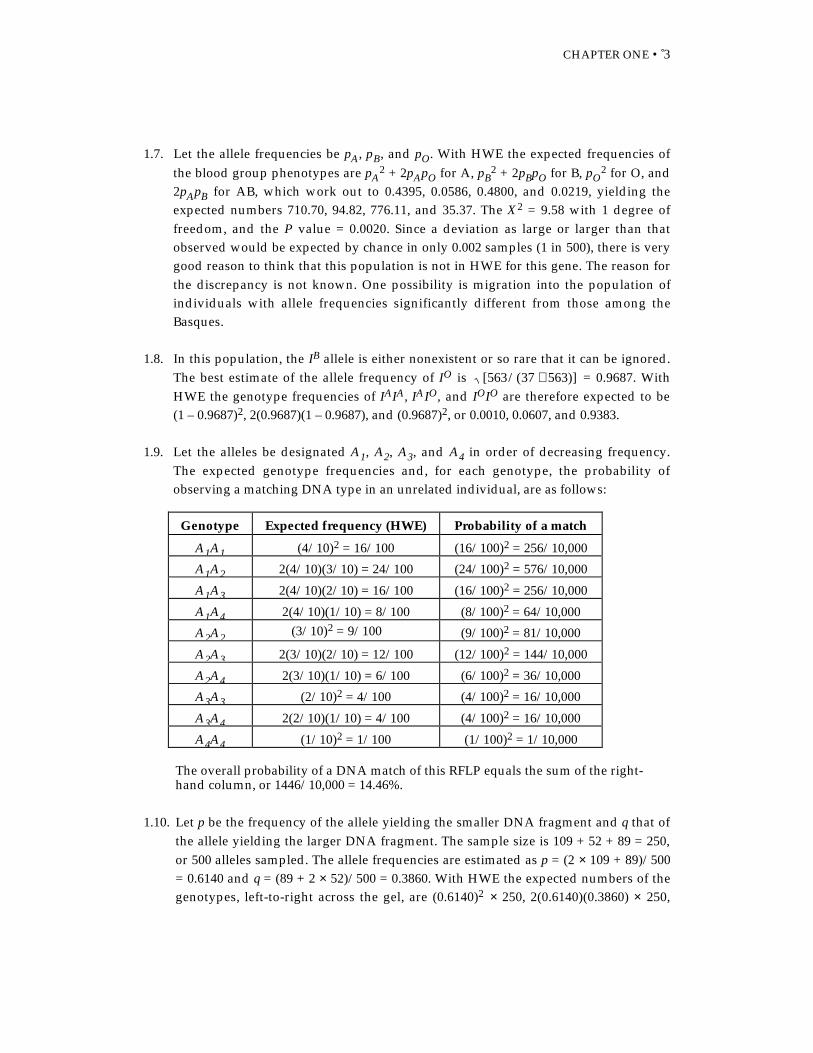
1.9. Let the alleles be designated A1, A2, A3, and A4 in order of decreasing frequency.The expected genotype frequencies and, for each genotype, the probability ofobserving a matching DNA type in an unrelated individual, are as follows:

Genotype Expected frequency (HWE) Probability of a match

A1A1 (4/10)2 = 16/100 (16/100)2 = 256/10,000

A1A2 2(4/10)(3/10) = 24/100 (24/100)2 = 576/10,000

A1A3 2(4/10)(2/10) = 16/100 (16/100)2 = 256/10,000

A1A4 2(4/10)(1/10) = 8/100 (8/100)2 = 64/10,000

A2A2 (3/10)2 = 9/100 (9/100)2 = 81/10,000

A2A3 2(3/10)(2/10) = 12/100 (12/100)2 = 144/10,000

A2A4 2(3/10)(1/10) = 6/100 (6/100)2 = 36/10,000

A3A3 (2/10)2 = 4/100 (4/100)2 = 16/10,000

A3A4 2(2/10)(1/10) = 4/100 (4/100)2 = 16/10,000

A4A4 (1/10)2 = 1/100 (1/100)2 = 1/10,000

The overall probability of a DNA match of this RFLP equals the sum of the right-hand column, or 1446/10,000 = 14.46%.

1.10. Let p be the frequency of the allele yielding the smaller DNA fragment and q that ofthe allele yielding the larger DNA fragment. The sample size is 109 + 52 + 89 = 250,or 500 alleles sampled. The allele frequencies are estimated as p = (2 × 109 + 89)/500= 0.6140 and q = (89 + 2 × 52)/500 = 0.3860. With HWE the expected numbers of thegenotypes, left-to-right across the gel, are (0.6140)2 × 250, 2(0.6140)(0.3860) × 250,

CHAPTER ONE • 4

and (0.3860)2 × 250, or 94.25, 37.25, and 118.50. The X2 = 15.50 with 1 degree offreedom, for which P = 0.000083. The null hypothesis of HWE must clearly berejected. The main reason for the poor fit is that there are too few observedheterozygous genotypes, relative to the number expected with HWE. A deficiencyof heterozygous genotypes might well be expected from inbreeding, and would beconsistent with some degree of self-fertilization. To estimate F, set 2pq(1 – F) × 250 =89, or 118.50(1 – F) = 89, yielding F = 0.2490. With this value of F, the expectednumbers agree perfectly with the observed, so there is no opportunity to do a chi-square test. The reason for the perfect fit is that both degrees of freedom wereconsumed in estimating p and F.

1.11. The RADP marker is X-linked, so (assuming HWE) the female genotype frequenciesare p2, 2pq, and q2 whereas the male genotype frequencies are p and q. In females qis estimated as [ /( )]102 967 102+ = 0.3089, and in males q is estimated as 346/(667+ 346) = 0.3416. The average of these is q = 0.3252. The expected numbers in femalesare 955.93 RAPD+ and 113.07 RAPD–; in males they are 683.54 RAPD+ and 329.46RAPD–. The X2 is 2.53 with 1 degree of freedom, and P = 0.112. There is no reasonto reject the null hypothesis of HWE for this X-linked DNA polymorphism.

1.12. Let A1 (allele frequency p1) and A2 (allele frequency p2) be, respectively, the alleleseither supporting or not supporting PCR amplification of the smaller band(bottom), and B1 (allele frequency q1) and B2 (allele frequency q2) be the alleleseither supporting or not supporting PCR amplification of the larger band (top). Thetotal number of haploid gametophytes sampled is 142 + 611 + 474 + 773 = 2000.a. The gametic frequencies are estimated as 142/2000 = 0.0710 for A1 B2, 611/2000

= 0.3055 for A2 B1, 474/2000 = 0.2370 for A1 B1, and 773/2000 = 0.3865 for A2 B2.Hence p1 = 0.0710 + 0.2370 = 0.3080 and p2 = 0.6920, and q1 = 0.0710 + 0.3055 =0.5425 and q2 = 0.4575. With LE the expected gametophyte frequencies, left-to-right across the gel, are p1q2 = 0.1409, p2q1= 0.3754, p1q1= 0.1671, and p2q2=0.3166, yielding the expected numbers 281.82, 750.82, 334.18, and 633.18. The X2

= 184.78 with 1 degree of freedom, and P≈0. The null hypothesis of LE issoundly rejected.

An alternative method of calculating X2 makes use of Equations 1.12 and1.13. Here D = (0.2370)(0.3865) – (0.0710)(0.3055) = 0.0699, hence the value ofρ = 0.0699/ [( . )( . )( . )( . )]0 3080 0 6920 0 5425 0 4575 = 0.3040. Then X2 = ρ2 × 2000 =184.78, confirming the previous value.

b. Since D = 0.0699 is positive, we want to compare it with Dmax, which is thesmaller of p1q2 and p2q1, which is to say the smaller of 0.1409 and 0.3754, whichequals 0.1409. Then D/Dmax = 0.0699/0.1409 = 0.50, or 50% of its maximumpossible value.

CHAPTER ONE • 5

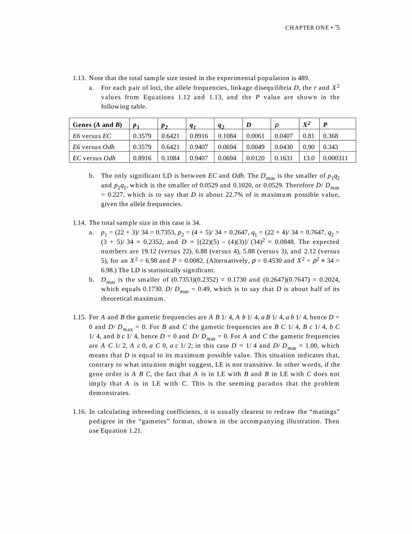
1.13. Note that the total sample size tested in the experimental population is 489.a. For each pair of loci, the allele frequencies, linkage disequilibria D, the r and X2

values from Equations 1.12 and 1.13, and the P value are shown in thefollowing table.

Genes (A and B) p1 p2 q1 q2 D ρ X2 P

E6 versus EC 0.3579 0.6421 0.8916 0.1084 0.0061 0.0407 0.81 0.368

E6 versus Odh 0.3579 0.6421 0.9407 0.0694 0.0049 0.0430 0.90 0.343

EC versus Odh 0.8916 0.1084 0.9407 0.0694 0.0120 0.1631 13.0 0.000311

b. The only significant LD is between EC and Odh. The Dmax is the smaller of p1q2and p2q1, which is the smaller of 0.0529 and 0.1020, or 0.0529. Therefore D/Dmax= 0.227, which is to say that D is about 22.7% of is maximum possible value,given the allele frequencies.

1.14. The total sample size in this case is 34.a. p1 = (22 + 3)/34 = 0.7353, p2 = (4 + 5)/34 = 0.2647, q1 = (22 + 4)/34 = 0.7647, q2 =

(3 + 5)/34 = 0.2352, and D = [(22)(5) – (4)(3)]/(34)2 = 0.0848. The expectednumbers are 19.12 (versus 22), 6.88 (versus 4), 5.88 (versus 3), and 2.12 (versus5), for an X2 = 6.98 and P = 0.0082. (Alternatively, ρ = 0.4530 and X2 = ρ2 × 34 =6.98.) The LD is statistically significant.

b. Dmax is the smaller of (0.7353)(0.2352) = 0.1730 and (0.2647)(0.7647) = 0.2024,which equals 0.1730. D/Dmax = 0.49, which is to say that D is about half of itstheoretical maximum.

1.15. For A and B the gametic frequencies are A B 1/4, A b 1/4, a B 1/4, a b 1/4, hence D =0 and D/Dmax = 0. For B and C the gametic frequencies are B C 1/4, B c 1/4, b C1/4, and b c 1/4, hence D = 0 and D/Dmax = 0. For A and C the gametic frequenciesare A C 1/2, A c 0, a C 0, a c 1/2; in this case D = 1/4 and D/Dmax = 1.00, whichmeans that D is equal to its maximum possible value. This situation indicates that,contrary to what intuition might suggest, LE is not transitive. In other words, if thegene order is A B C, the fact that A is in LE with B and B in LE with C does notimply that A is in LE with C . This is the seeming paradox that the problemdemonstrates.

1.16. In calculating inbreeding coefficients, it is usually clearest to redraw the “matings”pedigree in the “gametes” format, shown in the accompanying illustration. Thenuse Equation 1.21.

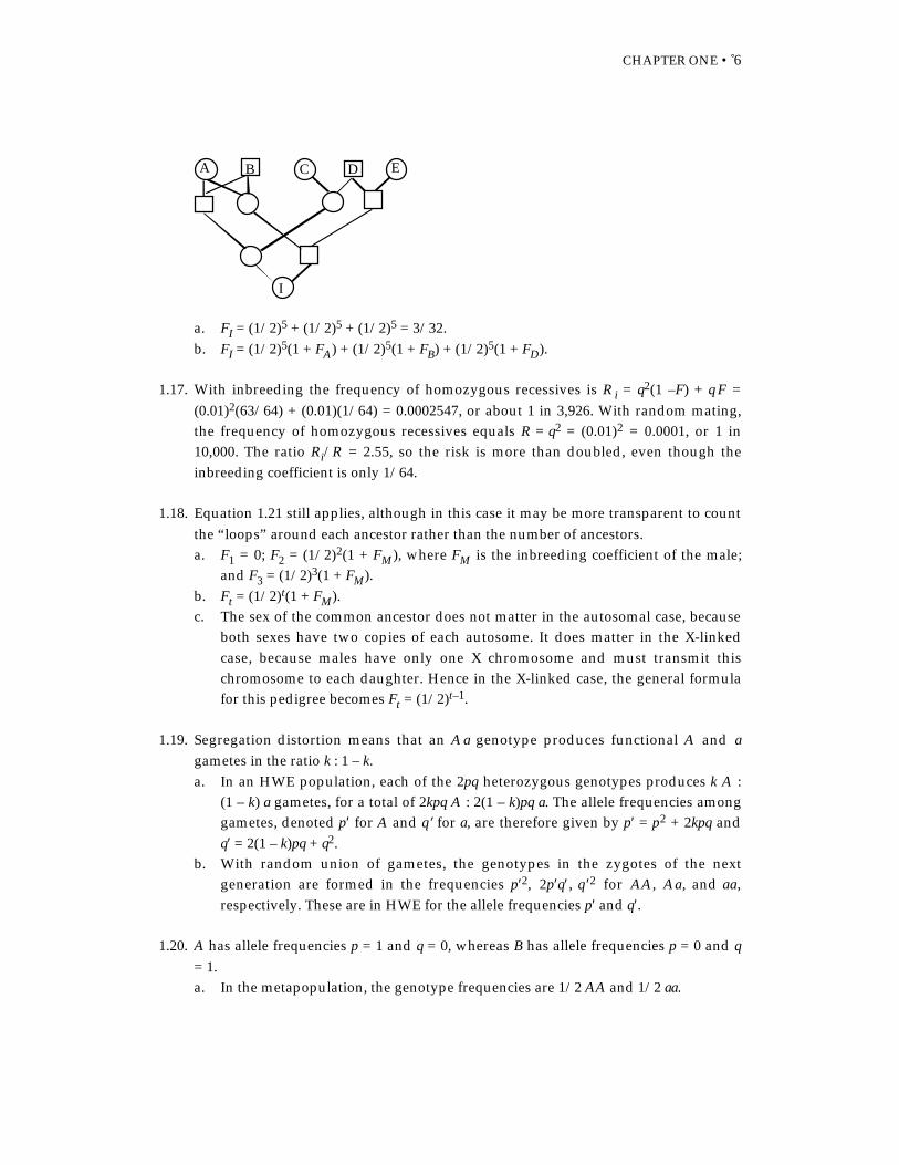
CHAPTER ONE • 6

A B C D E

I

a. FI = (1/2)5 + (1/2)5 + (1/2)5 = 3/32.b. FI = (1/2)5(1 + FA) + (1/2)5(1 + FB) + (1/2)5(1 + FD).

1.17. With inbreeding the frequency of homozygous recessives is R i = q2(1 –F) + q F =(0.01)2(63/64) + (0.01)(1/64) = 0.0002547, or about 1 in 3,926. With random mating,the frequency of homozygous recessives equals R = q2 = (0.01)2 = 0.0001, or 1 in10,000. The ratio Ri/R = 2.55, so the risk is more than doubled, even though theinbreeding coefficient is only 1/64.

1.18. Equation 1.21 still applies, although in this case it may be more transparent to countthe “loops” around each ancestor rather than the number of ancestors.a. F1 = 0; F2 = (1/2)2(1 + FM), where FM is the inbreeding coefficient of the male;

and F3 = (1/2)3(1 + FM).b. Ft = (1/2)t(1 + FM).c. The sex of the common ancestor does not matter in the autosomal case, because

both sexes have two copies of each autosome. It does matter in the X-linkedcase, because males have only one X chromosome and must transmit thischromosome to each daughter. Hence in the X-linked case, the general formulafor this pedigree becomes Ft = (1/2)t–1.

1.19. Segregation distortion means that an Aa genotype produces functional A and agametes in the ratio k : 1 – k.a. In an HWE population, each of the 2pq heterozygous genotypes produces k A :

(1 – k) a gametes, for a total of 2kpq A : 2(1 – k)pq a. The allele frequencies amonggametes, denoted p′ for A and q′ for a, are therefore given by p′ = p2 + 2kpq andq′ = 2(1 – k)pq + q2.

b. With random union of gametes, the genotypes in the zygotes of the nextgeneration are formed in the frequencies p′2, 2p′q′ , q ′2 for AA, Aa, and aa,respectively. These are in HWE for the allele frequencies p′ and q′.

1.20. A has allele frequencies p = 1 and q = 0, whereas B has allele frequencies p = 0 and q= 1.a. In the metapopulation, the genotype frequencies are 1/2 AA and 1/2 aa.

CHAPTER ONE • 7

b. After one (or more) generations of random mating, the genotype frequenciesare 1/4 AA, 1/2 Aa, and 1/4 aa.

c. There is a deficiency of heterozygous genotypes in the admixedmetapopulation, relative to the frequency expected with HWE.

d. Let A have allele frequencies p1 and q1 and B have allele frequencies p2 and q2.Then the metapopulation has a frequency of heterozygous genotypes equal toH = (2p1q1 + 2p2q2)/2. After one (or more) generations of random mating thefrequency of heterozygous genotypes equals H0 = 2[(p1 + p 2)/2][(q1 + q2)/2].Now calculate H – H0 = (p1q1 + p2q2) – [(p1 + p2)(q1 + q2)/2] = [(1 – q1)q1 + (1 –q2)q2] – [(2 – q1 – q2)(q1 + q2)/2] = q1 – q1

2 + q2 – q22 – q1 – q2 + q1

2/2 – 2q1q2/2 +q2

2/2 = –q12/2 – q2

2/2 + q1q2 = –(1/2)(q1 – q2)2. This must be negative unless q1= q2. In the next chapter we shall see that H0 – H equals the variance in allelefrequency among A and B.

CHAPTER TWO • 8

CHAPTER 2

2.1. Excision of the target sequence is an irreversible mutation process; hence Equation2.1 applies, with p0 = 1 for the initial frequency of the target sequence and µ = 0.01.The required answer is the smallest value of t for which qt

2 ≥ 0.05 because of HWE.Hence qt ≥ 0.2236 or p t ≤ 0.7764, which means that (1 – µ)t ≤ 0.7764 or t ≥[ln(0.7764)/ln(0.99)] = 25.18. Hence t = 26 generations is the required answer. Aquick check for verification shows that q25

2= 0.0493 whereas q262 = 0.0529.

2.2. The recombinational switch is formally equivalent to reversible mutation. ApplyEquation 2.5 with µ /(µ + ν) = 0.8453 and 1 – µ – ν = 0.9944. For initial p0 = 0, p30 =0.1302 (versus observed 0.16) and p700 = 0.8283 (versus observed 0.85). For initial p0= 1, p388 = 0.8631 (versus observed 0.88) and p700 = 0.8484 (versus observed 0.86).The fit to the observed values is very good. The predicted equilibrium frequency ofA is given by Equation 2.6 as 0.8453.

2.3. Haploid selection with constant fitnesses follows pt/qt = (p0/q0)(1 – s)–t (Equation2.27), where 1 – s is the fitness of the strain whose frequency is denoted q relative tothe fitness of the strain whose frequency is denoted p. In this problem, we are givenp0 and p35 and required to solve for 1 – s. The solution can be obtained from ln(1 – s)= [ln(p0/q0) – ln(pt/qt)]/t. For the gluconate data, ln(1 – s) = [ln(0.455/0.545) –ln(0.898/0.102)]/35 = –0.0673, or 1 – s = 0.9349, which indicates very strongselection favoring the strain with the allele gnd(RM43A). For the ribose data, ln(1 –s) = [ln(0.594/0.406) – ln(0.587/0.413)]/35 = 0.000827, or 1 – s = 1.00083, which iswithin experimental error from a relative fitness of 1.000.

2.4. Let the relative fitnesses of Cy/Cy, Cy/+, and +/+ be denoted w11, w12, and w22,respectively, where w22 = 1 and w11 = 0 is implied by the lethality of Cy/Cy. Theinitial frequency of the Cy allele, p = 0.168, is given. The frequency of the Cy allele inthe next generation is given by Equation 2.29.a. Here w1 2 = 1 and p′ = [(0.168)2(0)+(0.168)(0.832)(1)]/[(0.168)2(0) +

2(0.168)(0.832)(1) + (0.832)2(1)] = 0.1438.b. Here w12 = 0.5 and p′ = [(0.168)2(0)+(0.168)(0.832)(0.5)]/[(0.168)2(0) +

2(0.168)(0.832)(0.5) + (0.832)2(1)] = 0.0840.

2.5. Melanic moths result from a dominant allele. Therefore, with HWE, the frequencyof the recessive allele can be estimated as the square root of the proportion of

CHAPTER TWO • 9

nonmelanics. The data given are that t = 50 generations (1898–1850), q0 = ( . )1 0 01−= 0.9950, and q50 = ( . )1 0 95− = 0.2236.a. The change in frequency for a favored dominant allele is given by Equation

2.33, hence st = ln(pt/qt) + (1/qt) – ln(p0/q0) – (1/q0) = ln(0.7764/0.2236) +(1/0.2236) – ln(0.9950/0.0050) – ln(1/0.0050) = 10.0027, yielding s = 0.200.

b. If the melanic allele were recessive, we would have p0 = 0 01. = 0.1000 and pt =0 95. = 0.9747; s = 0.200 is given as the same selection coefficient as above. The

change in frequency of a favored recessive allele is given by Equation 2.35, sowe can write st = ln(pt/qt) – (1/pt) – ln(p0/q0) + (1/p0) = ln(0.9747/0.0253) –(1/0.9747) – ln(0.1000/0.9000) + (1/0.1000) = 14.8217. Therefore, t = 74.109generations.

2.6. A favored additive allele changes according to Equation 2.34, which with slightrearrangement reads ln(p0/q0) = ln(pt/qt) – st/2. In this application we set themutant allele frequency as q, and we are given that qt = 0.008 in 1965. To solve theproblem we must infer the initial frequency q0 from the frequency in 1965. For aninitial year 1950, which corresponds to t = 0, 1965 corresponds to t = 15 because weare told that that there is one generation per year. We also know that s = 0.20.Consequently, ln(p0/q0) = ln(0.9920/0.0080) – (0.20)(15)/2 = 3.3203, from which itfollows that q0 = 0.0349. (The observed value in 1950 was 0.037.) The initial year1940 makes t = 25, hence ln(p0/q0) = 2.3203, from which q0 = 0.0895. (The observedvalue in 1940 was 0.111).

2.7. Let the ST inversion be represented as A, and its “allele,” the AR inversion, berepresented as a. The relative fitnesses of AA, Aa, and aa are given as 0.47, 1.00, and0.62 (or wAA = 0.53 and w aa = 0.38, using the symbols in Equation 2.36). Theexpected equilibrium frequency of A is = 0.38/(0.53 + 0.38) = 0.4176, and theaverage fitness in the population at equilibrium is given by Equation 2.30 as(0.4176)2(0.47) + 2(0.4176)(0.5824)(1) + (0.5824)2(0.62) = 0.7787.

2.8 a. In the presence of warfarin the relative fitnesses of SS, SR, and RR are 0.68, 1.00,and 0.37. When written as 1 – wSS, 1.00, 1 – wRR, then wSS = 0.32 and wRR = 0.63.The stable equilibrium with overdominance is given by Equation 2.36 as p =wRR/(wSS + wRR) = 0.6632, which is the frequency of the S allele. The frequencyof the R allele is therefore 0.3368.

b. In the absence of warfarin the fitnesses of SS, SR, and RR are given by 1.00, 0.77,and 0.46, which with additive selection are written as 1.00, 1 – s/2, and 1 – s.The fitness of the heterozygous genotype yields s/2 = 0.23 or s = 0.46, whereasthe fitness of the homozygous R genotype yields s = 0.54. This is a reasonableapproximation of additive selection when s is taken as the mean, or s = (0.46 +0.54)/2 = 0.50, which yields relative fitnesses of 1.00, 0.75, and 0.50. The change

CHAPTER TWO • 10

in frequency of an additive allele is given by Equation 2.34; hence t =[ln(pt/qt) –ln(p0/q0)]/(s/2) = [ln(0.99/0.01) – ln(0.6632/0.3368)]/(0.25) = 15.67 generations.

2.9 a. At equilibrium for a complete recessive, q = µ /s = ( )/ .5 10 1 006× − =0.002236.

b. At equilibrium for a partial dominant, q = µ/hs = (5 × 10–6)/(0.025 × 1.00) =0.00020. Even though the relative fitness of the heterozygous genotype is 0.975,the partial dominance reduces the equilibrium allele frequency by a factor ofmore than 11.

2.10. Use Equation 2.9 with F0 = 0. For 1 – FST = 0.88, t is given by 0.88 = [1 – (1/2N)]t, or t= ln(0.88)/ln[1 – (1/2N)]. When N = 20, t = 5.0 generations, and when N = 100, t =25.5 generations.

2.11. Equation 2.9 with F0 = 0 applies again. The solution for N can readily be obtainedby rearranging the equation to read ln[1 – (1/2N)] = (1/t)ln( 1 – FST). We are given t= 45 and three values of FST. For Hawaii FST = 0.056 and N = 390.68; for AustraliaFST = 0.063 and N = 346.02; and for the combined data FST = 0.059 and N = 370.24.These estimates have relatively large sampling errors. Easteal (1985) has estimatedthe 95% confidence intervals as (119, 812), (104, 719), and (112, 770), respectively.

2.12. Use the harmonic mean 1/Ne = (1/t)∑(1/Ni) as in Equation 2.48. The estimated Ne =1/0.000254 = 3937.

2.13. Apply Equation 2.49 with Nm = 2 and Nf = 200. In this case Ne = 7.92, or only 3.9% ofthe actual population size.

2.14. Let qW , qC, and qE be the average frequency of the blue-color allele in the West,Central, and East regions, respectively, and qT be the overall average allelefrequency, weighting each population equally. Then qW = 3.092/6 = 0.5153, qC =0.254/11 = 0.0231, qE = 0.755/4 = 0.1888, and qT = 4.101/21 = 0.1953.a. The average subpopulation heterozygosity is the weighted average of the

regional heterozygosities, where the weight for each region equals the numberof subpopulations in the region. In effect, we treat the number of individuals ineach region as proportional to the number of subpopulationssampled. Therefore, HS = [6 × 2(0.5153)(1 – 0.5153) + 11 × 2(0.0231)(1 – 0.0231) +4 × 2(0.1888)(1 – 0.1888)]/21 = 0.2247. The total heterozygosity is the hetero-zygosity that would be expected were the population one large unit in HWE, orHT = 2(0.1953)(0.8047) = 0.3143.

b. FST = (HT – H S)/HT = 0.2851, which means that the population substructuredecreases the average frequency of heterozygous genotypes by almost 30% as

CHAPTER TWO • 11

compared with a single population in HWE.

2.15. For a deleterious recessive allele the average fitness at equilibrium equals 1 – q2swhere q = µ /s ; hence the reduction in average fitness from its value in theabsence of the mutation equals q2s = µ . For a partially dominant deleterious allelethe average fitness at equilibrium equals 1 – 2pqhs – q2s where q = µ/hs. To a verygood approximation p ≈ 1 and q2 ≈ 0 at equilibrium, hence the reduction in averagefitness from its value in the absence of the mutation equals approximately 2qhs = 2µ.

2.16. Equation 2.27 suggests how to proceed.a. Since pt/qt = (pt–1/qt–1)(1/wt–1), the method of successive substitutions yields

pt/qt = (p t–2/qt–2)(1/wt–1)(1/wt–2) = … = (p0/q0)(1/wt–1)(1/wt–2) … (1/w0) =p0/(q0w0w1 … wt–1).

b. Set wt = w0w1 … wt–1, from which it follows that w = (w0w1 … wt–1)1/t. This kindof average is called the geometric mean.

2.17. For a recessive lethal allele a, wAA = 1, w Aa = 1, and waa = 0. Then p′ is given byp′ = (p2 + pq)/(p2 + 2pq) = 1/(1 + q). Replacing p′ by 1 – q′ we obtain q′ = 1 – 1/(1 + q)= q/(1 + q). Writing qt for q′ and qt–1 for q yields qt = qt–1/(1 + qt–1) or 1/qt = 1 +1/qt–1. Since the relation between qt–1 and qt–2 is the same as that between qt andqt–1, it follows that 1/qt = 2 + 1/qt–2. Continuing in this manner we obtain 1/qt = t +1/q0 or, reinverting, qt = q0/(1 + tq0).

2.18. From Equation 2.29, p′ = [p2 + pq(1 – s)]/[p2 + 2pq(1 – s) + q2(1 – s)2] = p[p + q(1 –s)]/[p + q(1 – s)]2 = p/[p + q ( 1 – s)], and therefore q′ = q(1 – s)/[p + q (1 – s)]. Itfollows that p′/q′ = p/q(1 – s), which is identical to Equation 2.27 for a haploid withrelative fitnesses 1 : 1 – s.

2.19. Set 1 – 0.125 = 2(0.75 – 1)w12/(1 – 2w12) and solve for w12, which evaluates to 0.700.

2.20. At equilibrium ∂φ(x, t)/∂t = 0 because the function φ(x, t) no longer changes withtime. Therefore we need to show that φ(x) solves –dM(x)φ(x) / d x +(1/2)d2V(x)φ(x)/dx2 = 0. Here is the spirit of how Sewall Wright did it in 1938(Wright 1938). For compactness we will write φ, M, and V instead of φ(x), M(x), andV(x), and use prime (′) and double prime (′′ ) to denote first and second derivativeswith respect to x. In what follows C1, C2, C3, and C4 are constants of integration.

The argument is that, if φ solves –(Mφ)′ + (1/2)(Vφ)′′ = 0, then (1/2)(Vφ)′′ =(Mφ)′ or, integrating both sides over x, (1/2)(Vφ)′ + C1 = Mφ + C2. But C1 = 0 and C2= 0 because φ(x) = 0 for x = 0 and x = 1. Now divide both sides by Vφ, yielding(1/2)(Vφ)′/Vφ = M/V, then multiply both sides by 2 to obtain (Vφ)′/Vφ = 2M/V.But (Vφ)′/Vφ is the derivative of ln(Vφ); hence, integrating over both sides leads to

CHAPTER TWO • 12

ln(Vφ ) + C3 = C4 + 2∫(M/V)dx, or ln(Vφ ) = (C4 – C3) + 2∫(M/V)dx, from which wehave Vφ = C × exp[2∫(M/V)dx], where exp means “e raised to the power of” and C,which equals exp(C4 – C3), is a constant of integration chosen so that ∫φ(x)dx = 1.Therefore φ = (C/V) × exp[2∫(M/V)dx]. In this specific application, M/V = [(1 – x)ν –xµ]/[x(1 – x)/2N] and hence integrating 2∫(M/V)dx = ∫{(4Nν/x) – [4Nµ/(1 – x)]}dx =4Nν ln(x) + 4Nµ ln(1 – x). Therefore exp[2∫(M/V)dx] = x4Nν(1 – x)4Nµ, and finally,φ(x) = (C/V) × exp[2∫(M/V)dx] = C x4Nν–1 (1 – x)4Nµ–1.

Alternatively, one can start with the solution and do the differentiations bybrute force to show that –(M φ)′ + (1/2)(Vφ)′′ = 0. This approach is perfectlylegitimate, but not as elegant as Wright′s. (Incidentally, the value of the constant isC = Γ(4Nµ + 4Nν )/[Γ(4Nµ ) Γ(4Nν )] where Γ(·) is the gamma function.)

CHAPTER THREE • 13

CHAPTER 3

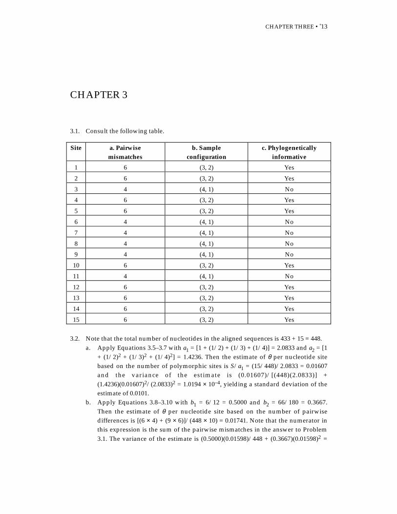
3.1. Consult the following table.

Site a. Pairwisemismatches

b. Sampleconfiguration

c. Phylogeneticallyinformative

1 6 (3, 2) Yes

2 6 (3, 2) Yes

3 4 (4, 1) No

4 6 (3, 2) Yes

5 6 (3, 2) Yes

6 4 (4, 1) No

7 4 (4, 1) No

8 4 (4, 1) No

9 4 (4, 1) No

10 6 (3, 2) Yes

11 4 (4, 1) No

12 6 (3, 2) Yes

13 6 (3, 2) Yes

14 6 (3, 2) Yes

15 6 (3, 2) Yes

3.2. Note that the total number of nucleotides in the aligned sequences is 433 + 15 = 448.a. Apply Equations 3.5–3.7 with a1 = [1 + (1/2) + (1/3) + (1/4)] = 2.0833 and a2 = [1

+ (1/2)2 + (1/3)2 + (1/4)2] = 1.4236. Then the estimate of θ per nucleotide sitebased on the number of polymorphic sites is S/a1 = (15/448)/2.0833 = 0.01607and the variance of the estimate is (0.01607)/[(448)(2.0833)] +(1.4236)(0.01607)2/(2.0833)2 = 1.0194 × 10–4, yielding a standard deviation of theestimate of 0.0101.

b. Apply Equations 3.8–3.10 with b1 = 6/12 = 0.5000 and b2 = 66/180 = 0.3667.Then the estimate of θ per nucleotide site based on the number of pairwisedifferences is [(6 × 4) + (9 × 6)]/(448 × 10) = 0.01741. Note that the numerator inthis expression is the sum of the pairwise mismatches in the answer to Problem3.1. The variance of the estimate is (0.5000)(0.01598)/448 + (0.3667)(0.01598)2 =

CHAPTER THREE • 14

1.3058 × 10–4, yielding a standard deviation of the estimate of 0.0114.

3.3. Use Equations 3.11–3.12 with c1 = 0.5000/2.0833 – 1/(2.0833)2 = 0.009600 and c2 =1/[(2.0833)2 + (1.4236)] × [(0.3667) – 7/[(2.0833)(5)] + (1.4236)/(2.0833)2] = 0.003933.The numerator in Equation 3.11 equals π – S/a1 = 0.01741 – 0.01607 = 0.001339 (seeProblem 3.2) and the denominator is the long radical shown in the next line

{( . )( / ) ( . )( / )[( / ) ( / )]}0 009600 15 448 0 003933 15 448 15 448 1 448+ − ,which equals 0.01804. Therefore Tajima’s D = 0.0742, which is very small andindicates no significant difference between the estimates of θ based on S/a1 orbased on π . (The data set is too small to make much of, in any case.) The fact that Dis positive indicates a slight excess of pairwise differences, suggesting that thepolymorphic nucleotides are a little more equally frequent than expected. Of coursethis is merely an illustrative example, and the excess is well within the range ofexperimental error.

3.4. For 12 sequences there are (12 × 11)/2 = 66 pairwise comparisons per alignednucleotide site.a. The minimum number of pairwise mismatches equals 11/66 when the

configuration is (11, 1); the maximum number of pairwise mismatches equals36/66 when the configuration is (6, 6).

b. Minimum 21/66 with configuration (10, 1, 1); maximum 48/66 withconfiguration (4, 4, 4).

c. Minimum 30/66 with configuration (9, 1, 1, 1); maximum 54/66 withconfiguration (3, 3, 3, 3).

3.5. The sequences of 18 aligned amino acids differ at 10 amino acid sites, hence D inEquation 3.27 is given by D = 10/18 = 0.5556, and therefore the corrected number ofreplacements per amino acid site is estimated as Ka = –ln(1 – D ) = 0.8109. Theestimated rate of amino acid replacement per amino acid site per year equals Ka/(2× 80 × 106) = 5.068 × 10–9. (The divergence time is doubled because an evolutionarybranch of 80 × 106 years extends to each species.) The standard deviation of Ka isgiven in Equation 3.27 as [ . /( . )]0 5556 0 4444 18× = 0.2635.

3.6. The separation of kangaroos and dogs took place 135 MYA. We are given the valueλ = 1 × 10–9 amino acid replacements per amino acid site per year. The proportionof amino acid sites in α-globin that are expected to differ is given by Equation 3.26as Dt = 1 – e–2λt = 0.2366. (The observed proportion is 0.234, so the fit to prediction isexcellent.)

3.7 a. The corrected amount of nucleotide divergence is given by Equation 3.28 as Kn= –(3/4)ln[1 – (4/3)D] where D = 9/60 = 0.1500 is the proportion of differences,

CHAPTER THREE • 15

hence Kn = 0.1674. The variance of Kn is given by (0.1500)(0.8500)/[(60)(1 –4D/3)2] = 0.003320, which yields a standard deviation of 0.05762. For aminoacids, the corrected divergence is given by Equation 3.27 as Ka = –ln(1 – D ),where D = 2/20 = 0.1000; hence Ka = 0.1053. The standard deviation is given by

[ /( ( )]D D20 1× − = 0.07453.b. Estimate λ from λ = K/2t where t is the divergence time, in this case 80 MY. For

nucleotide substitutions the estimated rate is λ = Kn/2t = 0.1674/(160 × 106) =1.0460 × 10–9 substitutions per nucleotide site per year. For amino acidreplacements the estimated rate is λ = Ka/2t = 0.1053/(160 × 106) = 0.6585 × 10–9

replacements per amino acid site per year.

3.8 a. The degeneracies are tabulated below. The amino acid sequence is given onlyfor E. coli ; the asterisks denote where it differs from that of S. typhimurium.Differences in the nucleotide sequences are underlined.

K12: V* A P I F I C P P N A D D D L L R Q I* AK12: GTCGCACCTATCTTCATCTGCCCGCCAAATGCCGATGACGACCTGCTGCGCCAGATAGCCLT2: ATCGCGCCGATCTTCATCTGCCCGCCAAATGCGGATGACGATCTTCTGCGCCAGGTCGCA 004004004002002002002004004002004002002002204004204002002004 N----S--S-----------------------S--------S--S---------N-N--S

b. Altogether there are 38 nonsynonymous sites, 12 twofold degenerate sites, and10 fourfold degenerate sites. The number of synonymous sites is calculated asthe number of fourfold degenerate sites plus 1/3 the number of twofolddegenerate sites, or 10 + (1/3)(12) = 14. The number of nonsynonymous sites isdefined as the number of nondegenerate sites plus 2/3 the number of twofolddegenerate sites, or 38 + (2/3)(12) = 46. The nucleotide substitutions areclassified as synonymous (S) or nonsynonymous (N) according to the criteriagiven in the problem in the line below the degeneracy assignments. There are 3nonsynonymous substitutions (even though there are only 2 amino acidreplacements) and 6 synonymous substitutions.

c. The 3 nonsynonymous substitutions yield Dn = 3/46 = 0.06522, and the 6synonymous substitutions yield Ds = 6/14 = 0.42857. Using Equation 3.28,which is appropriate for nucleotide data, the estimates are Kn = 0.0682nonsynonymous substitutions per nonsynonymous site and Ks = 0.6355synonymous substitutions per synonymous site. (It should be noted that thereis some loss of reliability when the correction for multiple hits is as large as it isin this example for synonymous sites.)

3.9. The problem specifies that the rate of divergence 2λ = 5–10 × 10–9 nucleotidesubstitutions per site per year, and that the average number of differences betweenmtDNA molecules is D = 0.0018. Equation 3.28 yields K = 0.001802 (the correction is

CHAPTER THREE • 16

actually unnecessary because D is so small), and because 2λt = K, the estimates oftime are t = 0.001802/(10 × 10–9) ≈ 180,000 years ago to 0.001802/(5 × 10–9) ≈ 360,000years ago. That is, the present mtDNA genetic diversity in this sample ofindividuals could have originated from a single mitochondrion present in a femaleas recently as 9,000–18,000 generations ago, assuming 20 years per generation.

One possible explanation of this finding is that the human population mighthave undergone a bottleneck in population size at about this time. In the popularpress, this conclusion has been interpreted as evidence for the existence of “Eve”(and, by implication, “Adam”). However, Equation 2.45 indicates that, amongneutral alleles destined to be fixed, the average time to fixation equals 4Negenerations. Assuming that a single mitochondrial genome became fixed in9,000–18,000 generations, and assuming that these values bracket the average, thecorresponding range of estimates of Ne for mitochondrial DNA (and therefore theNe of females) is 2250–4500, which is not unreasonable for small societies of the sortthat have characterized most of human evolution. Moreover, the average effectivesize of human populations in regard to mtDNA may not be representative of theaverage effective size in regard to nuclear DNA.

3.10 a. With Y = 1 – 0.20, w = 0.96852.b. (0.004/Z) = (1/0.96852) – (0.130/1.00) – 0.866 = 0.03650, hence Z = 0.10959 hence

1 – Z = 0.89041. This means that the β-galactosidase activity has to be reducedby 89% to produce the same fitness as that produced by a 20% decrease inpermease acivity.

c. The double mutant has a relative fitness of w = 0.93897. If the fitness reductionsof the single mutants (0.031477) were exactly additive, the fitness of the doublemutant would be expected to be 0.93706, which is quite close to the calculatedvalue.

3.11 a. There are 4146 nucleotides in the aligned region and 34 indels. The estimaterequired is K = –ln[1 – (34/4146)] = 0.008234 indels per nucleotide site.

b. For t = 34 MY, the rate of incorporation of indels equals λ = K/2t = 0.12110 ×10–9 indel substitutions per nucleotide site per year.

c. A rate of nucleotide sequence divergence of 1% per 2.2 MY corresponds to λ =0.01/(2.2 × 106) = 4.5455 × 10–9 substitutions per nucleotide site per year, whichis about 38-fold higher than the rate of indel substitution.

3.12. D is given as 0.15–0.20 which, from Equation 3.28 corresponds to K = 0.16736 –0.23262, and 2λt = K, where λ is the rate of sequence evolution given as λ = 5 × 10–9

per site per year. Hence the range of t values implied is t = 0.16736/(2 × 5 × 10–9) ≈16.7 MY to t = 0.23262/(2 × 5 × 10–9) = 23.3 MY.

CHAPTER THREE • 17

3.13 a. For IS1, the distribution in Equation 3.29 is given by p0 = 1/5 and p i =(4/5)(1/6)(5/6)i–1 for i ≥ 1. Hence the expected proportions are p0 = 0.2000, p1 =0.1333, p2 = 0.0111, p3 = 0.0926, p4 = 0.0772, and p≥5 = 1 – p0 – p1 – p2 – p3 – p4 =0.3858, yielding the expected number for 71 strains of 14.20, 9.47, 7.89, 6.57, 5.48,and 27.39, respectively. The X2 = 3.58 with 3 degrees of freedom and P = 0.311,so the fit is acceptable.

b. For IS2, p0 = 2/5 and pi = (3/5)(1/3)(2/3)i–1 for i ≥ 1. The expected numbersfrom 0 copies to ≥5 copies are 28.40, 14.20, 9.47, 6.31, 4.21, and 8.41, respectively.The X2 = 6.31 and P = 0.097, which is also acceptable.

c. For IS4, the distribution is given by p0 = 2/3 and pi = (1/3)(1/4)(3/4)i–1 for i ≥ 1.The expected numbers from 0 copies to ≥5 copies are 47.33, 5.92, 4.44, 3.33, 2.50,and 7.49, respectively. The X2 = 4.00 and P = 0.261, which is, once again,acceptable.

3.14. The X2 statistic for the chi-square test for independence (“homogeneity”) in a 2 × 2table with top-row entries a and b and bottom-row entries c and d can be shownfrom Equation 1.13 in Chapter 1 to equal (ad – b c)2N/[(a + b)(c + d)(a + c)(b + d)],where N = a + b + c + d. Alternatively, the expected values can be worked out fromthe marginal totals and the X2 calculated as ∑(observed – expected)2/expected in theusual way.a. Here a = 71, b = 106, c = 8, and d = 13, and X2 = 0.032 with 1 degree of freedom

for P = 0.858. In these data the ratio of amino acid fixations to amino acidpolymorphisms is not significantly different from the ratio of synonymousfixations to synonymous polymorphisms.

b. In this case, a = 60, b = 75, c = 20, and d = 44, yielding X2 = 3.14 and P = 0.076.Based on these data there is no reason to suggest that the ratio of synonymous-site fixations to polymorphisms is any different between boss and Adh.

3.15 a. The relevant quantity from the PRF model with s = 0 is the ratio of (4, 1) to (3, 2)configurations. Recall that the (4, 1) configuration includes both 4 ancestral : 1mutant and 4 mutant : 1 ancestral, because without additional information onecannot identify which nucleotide is “mutant” and which “ancestral.” Similarly,the (3, 2) configuration includes both 3 ancestral : 2 mutant and 2 mutant : 3ancestral. Hence the overall expected ratio of (4, 1) to (3, 2) is given by (1.00 +0.25) : (0.50 + 0.33) or 1.25 : 0.83. This implies that, among all polymorphicnucleotide sites in 5 aligned sequences, the expected proportion with the (4, 1)configuration is 0.6010 and that with the (3, 2) configuration 0.3990, assuming s= 0. For 27 polymorphisms, the expected numbers are 16.23 of (4, 1) and 10.77 of(3, 2), compared with the observed 17 and 10, respectively. The X2 = 0.093 with1 degree of freedom, and P = 0.760. The synonymous polymorphisms in thiscase do fit a model with no selection (s = 0), but it must be emphasized that the

CHAPTER THREE • 18

sample size is small.b. This can be solved by trial and error with the expected numbers 16.23 : 10.77.

Significance at the 5% level requires X2 > 3.841, which means that a fit withobserved numbers 11 : 16 or worse, as well as 22 : 5 or worse, will yield asignificant X2.

3.16 a. For Θ = 1, Pr{K2 = i} is given by (1/2)i+1 for i = 0, 1…. Hence, Pr{K2 = 0} = 1/2,Pr{K2 = 1} = (1/2)2 = 1/4, Pr{K2 = 2} = (1/2)3 = 1/8, and so forth.

b. The probability that two randomly chosen sequences are identical is Pr{K2 = 0}= 1/(1 + Θ).

c. The probability that two randomly chosen sequences differ at one of more sitesis Pr{K2 ≥ 1} = 1 – Pr{K2 = 0} = Θ/(1 + Θ). Equation 2.12 states that theequilibrium heterozygosity in the infinite-alleles model is given by theexpression H = θ/(1 + θ). The results are completely consistent because theinfinite-alleles model assumes that each mutation in a gene is unique, whereasthe infinite-sites model assumes that each mutation in a sequence ofnonrecombining nucleotides occurs at a different site.

d. Recombination increases the probability of one or more mismatches, since itincreases the numbers of ways in which two randomly chosen sequences candiffer. This can be appreciated by considering the case of free recombination.Suppose the sequence consists of n nucleotides and that the mutation rate persite is µ in a population of effective size N. Then the probability of identitybetweeen two random sequences at any one nucleotide is 1/(1 + 4Nµ), andtherefore with independence the probability of identity betweeen two randomsequences at all nucleotides is [1/(1 + 4Nµ)]n. Now (1 + 4Nµ)n = 1 + 4Nnµ + [n(n– 1)/2](4Nµ)2 + … ≥ 1 + 4NU, where U = nµ is the aggregate mutation rateacross all nucleotides. Since (1 + 4Nµ)n ≥ 1 + 4NU, it follows that [1/(1 + 4Nµ)]n

≤ 1/(1 + 4N U). This means that recombination decreases the probability ofidentity between randomly chosen pairs sequences, which implies that itincreases the probability of one or more mismatches.

3.17. Equation 3.3 states that Ti = 4N/[(i(i – 1)] (the overbar on Ti has been dropped fortypographical convenience).a. ∑Ti for i = 2 to 2N equals 4N{1/(1 × 2) + 1/(2 × 3) + 1/(3 × 4) + … + 1/[(2N – 1)

× 2N]} = 4N{1/2 + 1/6 + 1/12 + … + 1/[(2N – 1) × 2N]}.b. If there are 2N allele lineages in the population, then there are 2N coalescences

tracing all alleles back to a single common ancestral allele.c. The sum 1/2 + 1/6 + 1/12 + 1/20 + 1/30 + 1/42 + … goes to 1 as 2N becomes

large. For N = 50 it already equals 99/100, and for N = 500 it is 999/1000. [Thegeneral formula for the sum is (2N – 1)/2N].

CHAPTER FOUR • 19

CHAPTER 4

4.1. The mean µ = 100 and σ = 15. Note that µ + 2σ = 130. Since 95% of a normaldistribution is within the range µ ± 2σ, and since the normal distribution issymmetrical, 2.5% have phenotypic values ≤ µ – 2σ and 2.5% have phenotypicvalues ≥ µ + 2σ. Hence 2.5% have phenotypic values ≥ 130. Note that 85 is µ ± 1σ.Since 68% of the phenotypic values lie in the range µ ± 1σ, because of symmetry16% are ≤ µ – 1σ = 85. Hence 100% – 16% = 84% of the phenotypic values are ≥ 85.

4.2. The variance in the genetically heterogeneous population equals σg2 + σe

2 = 40,whereas that of the inbred lines is theoretically σe

2 = 10.a. The genotypic variance σg

2 is estimated as (σg2 + σe

2) – σe2 = 40 – 10 = 30, hence

the environmental variance is estimated as σe2 = 10. The broad-sense

heritability H2 is therefore estimated as H2 = 30/40 = 75%.b. The F1 from a cross of inbred lines is also genetically homogeneous, hence its

variance is theoretically σe2 = 10. In fact, the variance of the F1 tends to yield a

better estimate of σe2 than the variance of inbred lines, since inbred lines tend to

have a somewhat inflated variance due to the absence of heterozygosity.

4.3 a. The F1 generation yields an estimate of σe2.

b. The F2 generation yields and estimate of σg2 + σe

2.

4.4. The estimated σe2 = 1.46 and the estimated σg

2 = 5.97 – 1.46 = 4.51. The estimated H2

= 4.51/5.97 = 75.5%

4.5. From Equations 4.9 and 4.6, the additive genetic variance σa2 = 2pqα2 = 2pq[a + (q –

p)d]2. To apply this formula directly we must express the relative fitnesses ofST/ST, ST/AR, and AR/AR as +a, +d, and –a, respectively. It will be convenient todo this more generally, so let the relative fitnesses be written as wAA, wAa, and waa,in the same order as above. The quantity a equals the deviation of the phenotypicvalue of AA from the mean of that of the homozygous genotypes, hence a = wAA –(wAA + waa)/2 = (wAA – waa)/2. Similarly, –a is the deviation of the phenotypic valueof aa from the mean of that of the homozygous genotypes, or –a = waa – (wAA +waa)/2 = –(wAA –waa)/2. Likewise, d is the deviation of the phenotypic value of theheterozygous genotype from the mean of that of the homozygous genotypes, or d =wAa – (wAA + waa)/2 = (2wAa – wAA – waa)/2. In this specific case, wAA = 0.47, wAa =1.0, and waa = 0.62; hence a = –0.075 (it is all right for a to be negative and –a

CHAPTER FOUR • 20

positive) and d = 0.455.a. or p = 0 and p = 1, σa

2 = 2pqα2 = 0.b. For p = 0.2, σa

2 = 2(0.2)(0.8)[–0.075 + (0.8 – 0.2)(0.455)]2 = 0.012545, and for p =0.8, σa

2 = 0.038753.c. For p = 0.38/(0.53 + 0.38) = 0.41758242, σa

2 = 0.d. What is special about p = 0.38/(0.53 + 0.38) is that it is the stable equilibrium

with overdominance given by Equation 2.36 in Chapter 2, namely, p = (wAa –waa)/[(wAa – wAA) + (wAa – waa)] = 0.38/(0.53 + 0.38). What the result means isthat, at a genetic equilibrium, the genotypic variance can be ≠ 0 while theadditive variance can = 0. In fact, if the additive variance were ≠ 0 at anequilibrium, the point would not be an equilibrium, because the allelefrequencies would change due to natural selection.

4.6. The values of a and d are found as explained in the answer to Problem 4.5.a. For the proportions, a = 0.87 – (0.87 + 0.44)/2 = 0.435 and d = 0.44 – (0.87 +

0.44)/2 = 0.005, and the degree of dominance equals d/a = 0.01149; hence thealleles are nearly additive.

b. For the arcsin x transformation, a = 34.435, d = 7.115, and d/a = 0.20662. Onthis scale the cr pigmentation allele is partially dominant. Which scale ofmeasurement is the one to use? Whichever one yields a normal distribution ofthe phenotypic values.

4.7. With this distribution, the phenotypic values 0–8 occur with probabilities0.00390625, 0.0313, 0.1094, 0.2188, 0.2734, 0.2188, 0.1094, 0.03125, and 0.00391,respectively.a. The mean equals (0.00391)(0) + (0.0313)(1) + … = 4. The direct calculation is

unnecessary because the mean of a binomial distribution of n elements withrespective probabilities p and 1 – p equals np = (8)(1/2) = 4. The variance equals(0.00391 – 2)2(0) + (0.0313 – 2)2(1) + … = 2. No direct calculation is necessaryhere, either, because the variance of a binomial distribution of n elements withrespective probabilities p and 1 – p equals np(1 – p) = (8)(1/2)(1/2) = 2.

b. Among individuals with phenotypic values of 6, 7, or 8, the relative proportionsare 0.1094 : 0.03125 : 0.00391. These must be normalized to equal 1 by dividingby their total (0.14453), yielding the probabilities 0.7568 (phenotypic value 6),0.21622 (phenotypic value 7), and 0.02703 (phenotypic value 8), which now sumto 1. The mean of this group equals (0.7568)(6) + (0.21622)(7) + (0.02703)(8) =6.27027; hence the selection differential S = µS – µ = 6.27027 – 2.00000 = 4.27027.

c. With a narrow-sense heritability of h2 = 50%, the expected response to selectionR is given by R = µ′ – µ = h2S = (0.50)(4.27027) = 2.13514; hence the expectedvalue of µ′ = 4.13514.

CHAPTER FOUR • 21

4.8 a. Compare R = h2S with R = iσph2, from which it is clear that iσp = S or i = S/σp.Hence i equals the selection differential S expressed in multiples of thephenotypic standard deviation σp.

b. Any normal distribution can be transformed into a “standard” normaldistribution with mean 0 and variance 1 by means of the transformation y = (x –µ)/σ. A truncation point of T in the original distribution is transformed into thetruncation point t = (T – µ)/σ in the standard normal distribution. However, theproportion of the population saved for breeding, B, remains the same under thetransformation. Hence S = (µS – µ)/σp depends only on B.

4.9. The relevant means are µ = 19.304 of the G1 generation, µS = 22.727 of the selectedparents, and µ′ = 20.149 of the G2 generation. Therefore, S = 22.727 – 19.304 = 3.4229is the selection differential and R = 20.149 – 19.304 = 0.8442 is the response, yieldinga realized heritability of h2 = R/S = 0.2466.

4.10 a. The mean of the variances of the parental inbred lines equals (0.00142 +0.00053)/2 = 0.000975, which is an estimate of σe

2, hence an estimate of σg2 =

0.00303 – 0.000975 = 0.002055. The difference between the means of the inbredlines is D = 0.609, and so the Wright-Castle index is n = D2/(8σg

2) = 22.56.b. Estimating σe

2 as the F1 variance yields σe2 = 0.0003, from which σg

2 isestimated as 0.00273. In this case, n = 16.98.

4.11. This principle can be demonstrated by the method of successive substitutions usingµ′ – µ = Sh2. Because we are dealing with a population across multiple generations,it is best to use generational subscripts rather than µ′ and µ. The initial generationhas mean µ0 and the selection differential in this generation is S0; hence µ1 – µ0 =S0h2. By the same logic µ2 – µ1 = S1h2. Adding these two equations yields µ2 – µ0 =(S0 + S1)h2. Note that the µ1 terms have cancelled. Now µ3 – µ2 = S2h2, and addingthis to the previous equation yields µ3 – µ0 = (S0 + S1 + S2)h2, where now the µ2terms have cancelled. Continuing in this manner yields the desired formula µn – µ0= (S0 + S1 + … + Sn–1)h2. This equation does not hold if h2 changes during thecourse of the selection, because then we would have µn – µ0 = S0h0

2 + S1h12 + … +

Sn–1hn–12.

4.12. Use the formula given in Problem 4.11. We are given µ76 = 18.8% and µ0 = 4.8%. Thestatement that the cumulative selection differential increased by an approximatelyconstant amount of 1.1 per generation implies that S0 ≈ 1.1, S1 ≈ 1.1, S2 ≈ 1.1, and soforth. After 76 generations of selection the cumulative selection differential equals76 × 1.1 = 83.6 and the total response equals 18.8 – 4.8 = 14.0. The realizedheritability across 76 generations is therefore h2 = 14.0/83.6 = 16.75%. It should benoted that the selection was for entire ears, not individual kernels, based on the

CHAPTER FOUR • 22

average oil content of the kernels in each ear. Since kernels on the same ear arerelated as half-siblings (because they have the same mother plant but differentpollen donors), the realized heritability is actually the realized heritability of half-sib family means.

4.13. This kind of problem is well-suited to calculations using any standard spreadsheetprogram, as the calculations are rather tedious when carried out by hand. Thevalues needed are the variance of midparent values, which equals 8.17993 mm2,and the covariance between midparent values and offspring means, which equals5.18310 mm2. The narrow-sense heritability h2 is estimated as the regressioncoefficient b = 5.18310/8.17993 = 0.634, or 63.4%. There is some loss of accuracyfrom grouping the data into categories. The regression coefficient for theungrouped data is b = 0.70. It should also be noted that there is substantialassortative mating for shell breadth, which inflates the estimate of the narrow-senseheritability.

4.14 a. w = p2wAA + 2pqwAa + q2waa and so dw /dp = 2pwAA – 2pwAa + qwAa – 2qwaa =2[p(wAA – wAa) + q(wAa – waa)]. The numerator in Equation 2.31 is pq[p(wAA –wAa) + q(wAa – waa)]. Using the chain rule given in the problem, dw /dt = dw /dp× dp/dt = 2pq[p(wAA – wAa) + q(wAa – waa)]

2.b. See the answer to Problem 4.5, where it is shown that a = wAA – (wAA + waa)/2 =

(wAA – waa)/2 and d = wAa – (wAA + waa)/2 = (2wAa – wAA – waa)/2.c. α = a + (q – p)d = [(p + q)(wAA + wAa)/2] – [(q – p)(2wAa – wAA – waa)/2] = p(wAA

– wAa) + q(wAa – waa).d. dw /dt = 2pqα2, which says that the increase in average fitness in the population

at any time equals the additive genetic variance in fitness at that time. This isFisher′s principle of the “fundamental theorem of natural selection.”

4.15. For a recessive allele, d = a, so α = a + (q – p)a = 2qa. Therefore σa2 = 2pqα2 = 8pq3a2

and σd2 = (2pqd)2 = 4p2q2a2. Then set h2 = σ a

2/(σa2 + σd

2), which reduces to theexpression 2q/(1 + q).

4.16. In this case, d = –a. Then σa2 = 8p3qa2 and σd

2 = (2pqd)2 = 4p2q2a2. Then set h2 =σa

2/(σa2 + σd

2), which reduces to 2(1 – q)/(2 – q).

4.17. The narrow-sense heritability depends on the parent-offspring correlation and noton the sibling correlation (see Table 4.4). For a trait determined by a rare recessiveallele, the parent-offspring correlation goes to 0 as q goes to 0, because parent andoffspring will not both be affected. This is because affected offspring will come onlyfrom heterozygous × heterozygous matings. For a trait determined by a raredominant allele, on the other hand, the parent-offspring correlation increases to a

CHAPTER FOUR • 23

maximum as q goes to 0, because all affected offspring will have one affectedparent.

4.18. Table 4.2 gives the deviations from the population mean of AA , AA ′ , and A ′A′genotypes as 2qα – 2q2d, (q – p)α + 2pqd, and –2pα – 2p2d, respectively. These are they values in the regression. The corresponding x values are 2, 1, and 0, respectively,and the frequencies of the pairs are p2, 2pq, and q2; hence the x population mean is2p2 + 2pq = 2p and the deviations of the x values are 2 – 2p = 2q, 1 – 2p = (q – p), and0 − 2p = –2p, respectively. The covariance between x and y equals p2(2q)(2qα – 2q2d)+ 2pq(q – p)[(q – p)α + 2pqd] + q2(–2p)(–2pα – 2p2d).

This is best approached term by term. The coefficient of the α term is 4p2q2 +2pq(q – p)2 + 4p2q2 = 2pq(2pq + q2 – 2pq + p2 + 2pq) = 2pq(p + q)2 = 2pq. The coefficientof the d term is –4p2q3 + 4p2q2(q – p) + 4p3q2 = 4p2q2(–q + q – p + p) = 0. Hence thecovariance equals 2pqα. The variance of the x values is p2(2q)2 + 2pq(q – p)2 +q2(–2p)2 = 2pq (2pq + q2 – 2pq + p2 + 2pq) = 2pq. Hence the regression coefficient ofphenotype on number of A alleles equals 2pqα/2pq = α.

4.19. The calculations can be organized systematically by means of the following table.

Mother Frequency Deviation Sons Frequency Deviation

AA p2 2qα – 2q2d A 1 2qa

AA′ 2pq (q – p)α + 2pqd A 1/2 2qa

A′ 1/2 –2pa

A′A′ q2 –2pα – 2p2d A′ 1 –2pa

In this table, the deviations for the females are those in Table 4.2. The deviations inthe sons are derived from the fact that the mean phenotypic value among sonsequals p2a + pqa + pq(–a) + q2(–a) = (p – q)a; hence the deviation for A males is a – (q –p)a = 2qa and that for A ′ males is –a – (q – p )a = –2pa. The mother-son covarianceequals p2(2qα – 2q2d)(2qa) + pq[(q – p)α + 2pqd](2qa) + pq[(q – p)α + 2pqd](–2p) +q2(–2pα – 2p2d)(–2p), which it is best to work out term by term. The results are thatthe coefficient of aα is 2p2q2 while that of ad is 0. Hence the covariance betweenmothers and their sons for an X-linked gene equals 2p2q2aα.

4.20. The mean parental phenotype equals p1 + p2, so the deviations of the parents in theparent-offspring pairs are, from top to bottom, 1 – (p1 + p2), 1 – (p1 + p2), –(p1 + p2),and –(p1 + p2). Note that p1 + p2 = b, the proportion of affected individuals in the

CHAPTER FOUR • 24

population. In terms of b the deviations can be written as 1 – b, 1 – b, –b, and –b,respectively, so the variance among the parents equals p1(1 – b)2 + p2(1 – b)2 +p3(–b)2 + p4(–b)2 = b(1 – b)2 + (1 – b)b2 = b – b2. The offspring mean equals p1 + p3,which also equals b, and the deviations, from top to bottom, are 1 – b, –b, 1 – b, and–b. The parent-offspring covariance is therefore equal to p1(1 – b)(1 – b) + p2(1 –b)(–b) + p3(–b)(1 – b) + p4(–b)(–b) = p1 – b(2p1 + p2 + p3) + b2 = p1 – b2 (because 2p1 + p2+ p3 = 2b). The regression coefficient is therefore (p1 – b2)/(b – b2), which if b2 ≈ 0becomes p1/b. In terms of conditional probabilities, p1 = Pr{O|P}Pr{P} = Pr{O|P}b;hence the regression coefficient in terms of conditional probabilities equals Pr{O|P},which is the “trait heritability.” It is a very different thing than the heritability ofliability.

4.21. The log10(BR) = log10(0.025) = –1.60206 and log10(BG) = log10(0.004) = –2.39794.Equation 4.36, after some rearrangement, yields a quadratic formula in the variableh2, which has two solutions, h2 ≈ –1.272987, which is biologically impossible, and h2

= 0.456501, which is the estimate of narrow-sense heritability of liability.a. For brothers or sisters of affected individuals, use Equation 4.36 with h2 =

0.456501; hence log10(BR) = –1.60206 or BR = 0.02500, or about 1 in 40.b. For nephews or nieces of affected individuals, use Equation 4.36 with h2 =

0.456501/2; hence log10(BR) = –1.97205 or BR = 0.01066, or about 1 in 94.c. For cousins of affected individuals, use Equation 4.36 with h2 = 0.456501/4;

hence log10(BR) = –2.17735 or BR = 0.00665, or about 1 in 150.