i

İSTANBUL TECHNICAL UNIVERSITY ���� INSTITUTE OF SCIENCE AND TECHNOLOGY

A PRICE-SENSITIVE QUANTITY-FLEXIBLE

SUPPLY CHAIN CONTRACT MODEL

AS A SUPPLY CHAIN PERFORMANCE DRIVER

Ph.D. Thesis by

Murat ÖZMIZRAK, M.Sc.

(507802018)

Supervisor (Chairman): Prof. Dr. Semra BİRGÜN

Members of the Examining Committee Assoc. Prof. Dr. Mehmet TANYAŞ

Assoc. Prof. Dr. Tijen ERTAY

Prof. Dr. Sami ERCAN (İTİCÜ)

Prof. Dr. Alpaslan FIĞLALI (KÜ)

Date of submission: 30 January 2006

Date of defence examination: 30 June 2006

JUNE 2006

ii

İSTANBUL TECHNICAL UNIVERSITY ���� INSTITUTE OF SCIENCE AND TECHNOLOGY

FİYATA DUYARLI VE MİKTAR ESNEKLİĞİ OLAN BİR

TEDARİK ZİNCİRİ SÖZLEŞME MODELİNİN

TEDARİK ZİNCİRİ PERFORMANS GELİŞTİRİCİSİ OLARAK KULLANIMI

DOKTORA TEZİ

Murat ÖZMIZRAK, M.Sc.

(507802018)

Tez Danışmanı: Prof. Dr. Semra BİRGÜN

Diğer Jüri Üyeleri Doç. Dr. Mehmet TANYAŞ

Doç. Dr. Tijen ERTAY

Prof. Dr. Sami ERCAN (İTİCÜ)

Prof. Dr. Alpaslan FIĞLALI (KÜ)

Tezin Enstitüye Verildiği Tarih: 30 Ocak 2006

Tezin Savunulduğu Tarih: 30 Haziran 2006

HAZİRAN 2006

iii

ACKNOWLEDGEMENTS

One of the great pleasures of writing a dissertation is acknowledging the efforts of

many people whose cooperation and understanding were crucial.

I would first like to express my sincere gratitude to my supervisor Prof. Dr. Semra

Birgün for her guidance and support throughout my graduate studies. Her insight,

encouragement, and direction provided an exceptional foundation for this

dissertation. I was certainly fortunate to have her as my supervisor.

I would also like to thank the members of my committee, Prof. Dr. Sami Ercan,

Prof. Dr. Alpaslan Fığlalı, Assoc. Prof. Dr. Mehmet Tanyaş, and Assoc. Prof. Dr.

Tijen Ertay for their valuable input during all stages of this dissertation. Their help is

gratefully acknowledged.

Several other faculty and institute members enhanced my experience at İstanbul

Technical University. I shall not attempt to thank all of them by name as I would

surely miss someone, but their support is certainly appreciated.

To my parents Emel and İlhan Özmızrak and my brother Suat Özmızrak, whose

lifetime love are unshakeable, I owe a deep dept of gratitude. The same goes to my

other parents and brother, İhsan and Jale Kesen and Dr. Yavuz Kesen, and my late

aunt Esma Deniz whose support and perseverance were truly outstanding.

Finally, I would like to thank my best friend and wife Dr. Fatma Nur Özmızrak for her

exceptional encouragement and lifetime love and support, and my wonderful

daughter Feriha Pınar Özmızrak for giving me every reason to smile every day.

I love you all.

June 2006 Murat Özmızrak

iv

TABLE OF CONTENTS

ABBREVIATIONS vii

LIST OF TABLES viii

LIST OF FIGURES ix

LIST OF SYMBOLS x

SUMMARY xi

TÜRKÇE ÖZET xiii

CHAPTER 1. INTRODUCTION 1

1.1 Supply Chain Contracts and Committed Delivery Strategies 2 1.2 Overview 2

CHAPTER 2. LITERATURE REVIEW 5

CHAPTER 3. SUPPLY CHAIN MANAGEMENT 12

3.1 Decision Phases in a Supply Chain 13 3.1.1 Supply Chain Strategy 13 3.1.2 Supply Chain Planning 13 3.1.3 Supply Chain Operation 14

3.2 Process View of a Supply Chain 14 3.2.1 Cycle View 14

3.2.1.1 Customer Order Cycle 15 3.2.1.2 Replenishment Cycle 16 3.2.1.3 Manufacturing Cycle 17 3.2.1.4 Procurement Cycle 18

3.2.2 Push/Pull View 19 3.3 How to Implement Supply Chain Management 19

CHAPTER 4. SUPPLY CHAIN PERFORMANCE 22

4.1 Competitive and Supply Chain Strategies 22 4.2 Strategic Fit 22

4.2.1 Understanding the Customer 23 4.2.2 Understanding the Supply Chain 24 4.2.3 Achieving Strategic Fit 26

4.2.3.1 Multiple Products and Customer Segments 28 4.2.3.2 Product Life Cycle 28 4.2.3.3 Competitive Changes over Time 29

4.3 Expanding Strategic Scope 29 4.3.1 Intracompany Intraoperation Scope: The Minimize Local Cost View 30 4.3.2 Intracompany Intrafunctional Scope: The Minimize Functional Cost View 31 4.3.3 Intracompany Interfunctional Scope: The Maximize Company Profit View 31

v

4.3.4 Intercompany Interfunctional Scope: The Maximize Supply Chain Surplus View 32 4.3.5 Flexible Intercompany Interfunctional Scope 32

4.4 Demand Driven Supply Chain 32 4.5 Supply Chain Performance Drivers 35

4.5.1 Inventory 36 4.5.1.1 Role in the Supply Chain 36 4.5.1.2 Role in the Competitive Strategy 37 4.5.1.3 Components of Inventory Decisions 37

4.5.2 Transportation 38 4.5.2.1 Role in the Supply Chain 38 4.5.2.2 Role in the Competitive Strategy 38 4.5.2.3 Components of Transportation Decisions 39

4.5.3 Facilities 39 4.5.3.1 Role in the Supply Chain 40 4.5.3.2 Role in the Competitive Strategy 40 4.5.3.3 Components of Facilities Decisions 40

4.5.4 Information 41 4.5.4.1 Role in the Supply Chain 41 4.5.4.2 Role in the Competitive Strategy 42 4.5.4.3 Components of Information Decisions 42

4.6 Obstacles to Achieving Strategic Fit 43 4.6.1 Increasing Variety of Products 43 4.6.2 Decreasing Product Life Cycles 44 4.6.3 Increasingly Demanding Customers 44 4.6.4 Fragmentation of Supply Chain Ownership 44 4.6.5 Globalization 44 4.6.6 Difficulty in Executing New Strategies 45

4.7 Managing Predictable Variability 45 4.7.1 Managing Supply 46 4.7.2 Managing Demand 46

4.8 Implications of Supply Chain Management in Agile Manufacturing 47

CHAPTER 5. INFORMATION TECHNOLOGY STRUCTURE AND SUPPLY CHAIN CONTRACTS 49

5.1 Information Networks 49 5.1.1 Information System Functionality 49 5.1.2 Communication Systems 50

5.2 Enterprise Resource Planning (ERP) and Execution Systems 51 5.2.1 Rationale for ERP Implementation 52 5.2.2 Enterprise Execution Systems 53

5.2.2.1 Customer Relationship Management (CRM) 53 5.2.2.2 Transportation Management System (TMS) 53 5.2.2.3 Warehouse Management System (WMS) 54

5.3 Advanced Planning and Scheduling (APS) 54 5.3.1 Rationale for Advanced Planning and Scheduling 55

5.3.1.1 Planning Horizon Recognition 55 5.3.1.2 Supply Chain Visibility 56 5.3.1.3 Simultaneous Resource Consideration 56 5.3.1.4 Resource Utilization 57

5.3.2 Supply Chain APS Applications 57 5.3.2.1 Demand Planning 57 5.3.2.2 Production Planning 58 5.3.2.3 Requirements Planning 59 5.3.2.4 Transportation Planning 59

vi

5.3.3 APS System Components 59 5.3.3.1 Demand Management 60 5.3.3.2 Resource Management 60 5.3.3.3 Resource Optimization 61 5.3.3.4 Resource Allocation 62

5.3.4 Collaborative Planning, Forecasting, and Replenishment (CPFR) 62 5.3.5 APS Benefits and Considerations within the Supply Chain Contracts Context 64

CHAPTER 6. SUPPLY CONTRACTS AND COMMITTED DELIVERY STRATEGIES 66

6.1 Retailer Profit without Commitment Opportunity with Demand as a Function of the Selling Price 67 6.2 Retailer Profit with Commitment Opportunity with Demand as a Function of the Selling Price 71

6.2.1 Pricing and Profit Implications of Committed Delivery Strategies 72 6.3 Retailer Profit without Commitment Opportunity with Normally Distributed Demand 73

6.3.1 Expected Profit from an Order 74 6.3.2 Expected Overstock from an Order 75 6.3.3 Expected Understock from an Order 75

6.4 Supply Chain Surplus 75 6.5 Buyback Contracts 76 6.6 Quantity Flexibility Contracts 78

CHAPTER 7. PROPOSED SUPPLY CHAIN CONTRACT MODEL 81

7.1 Profit Sharing while Maximizing the Supply Chain Surplus 81 7.1.1 Profit Sharing with β as a Parameter 83 7.1.2 Profit Sharing with Wholesale Price as a Parameter 84

7.2 Committed Deliveries using Quantity Flexibility Contracts to Maximize Supply Chain Surplus with Demand as Function of the Selling Price 86 7.3 Computer Program to Find Optimum Contract Parameters 94

7.3.1 Simulate_p 94 7.3.2 Simulate_alpha 96 7.3.3 Simulate_p_alpha 97 7.3.4 Simulate_c and Simulate_beta 97

7.4 Model Comparison 99

CHAPTER 8. CONCLUSION AND DIRECTIONS FOR FUTURE RESEARCH 101

8.1 Future Work 102

BIBLIOGRAPHY 103

APPENDIX A. EXCEL CALCULATIONS 118

VITA 121

APPENDIX B. VBA COMPUTER PROGRAMS CD

vii

ABBREVIATIONS

APS : Advanced Planning and Scheduling ATP : Available To Promise CPFR : Collaborative Planning, Forecasting, and Replenishment CRM : Customer Relationship Management CTP : Capable To Promise EDI : Electronic Data Interchange ERP : Enterprise Resource Planning GSCM : Global Supply Chain Management ISCM : Integrated Supply Chain Management IT : Information Technology JIT : Just-In-Time MRP : Material Requirements Planning MRP II : Manufacturing Resource Planning SCIS : Supply Chain Information Systems SCM : Supply Chain Management SKU : Stock Keeping Unit TMS : Transportation Management System VAS : Value Added Services VBA : Visual Basic for Applications VMI : Vendor Managed Inventories WMS : Warehouse Management System XML : Extensible Markup Language

viii

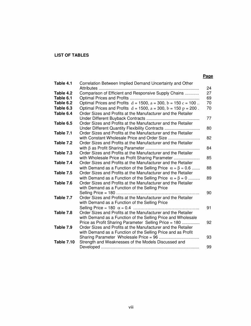
LIST OF TABLES

Page

Table 4.1 Correlation Between Implied Demand Uncertainty and Other Attributes ..................................................................................... 24

Table 4.2 Comparison of Efficient and Responsive Supply Chains ............ 27 Table 6.1 Optimal Prices and Profits ........................................................... 69 Table 6.2 Optimal Prices and Profits d = 1500, a = 300, b = 150 c = 100 .. 70 Table 6.3 Optimal Prices and Profits d = 1500, a = 300, b = 150 p = 200 . 70 Table 6.4 Order Sizes and Profits at the Manufacturer and the Retailer

Under Different Buyback Contracts ............................................. 77 Table 6.5 Order Sizes and Profits at the Manufacturer and the Retailer

Under Different Quantity Flexibility Contracts .............................. 80 Table 7.1 Order Sizes and Profits at the Manufacturer and the Retailer

with Constant Wholesale Price and Order Size ........................... 82 Table 7.2 Order Sizes and Profits at the Manufacturer and the Retailer

with β as Profit Sharing Parameter .............................................. 84 Table 7.3 Order Sizes and Profits at the Manufacturer and the Retailer

with Wholesale Price as Profit Sharing Parameter ...................... 85 Table 7.4 Order Sizes and Profits at the Manufacturer and the Retailer

with Demand as a Function of the Selling Price α = β = 0.6 ....... 88 Table 7.5 Order Sizes and Profits at the Manufacturer and the Retailer

with Demand as a Function of the Selling Price α = β = 0 .......... 89 Table 7.6 Order Sizes and Profits at the Manufacturer and the Retailer

with Demand as a Function of the Selling Price Selling Price = 180 ………………………………………………….. 90

Table 7.7 Order Sizes and Profits at the Manufacturer and the Retailer with Demand as a Function of the Selling Price Selling Price = 180 α = 0.4 ……………………………………….. 91

Table 7.8 Order Sizes and Profits at the Manufacturer and the Retailer with Demand as a Function of the Selling Price and Wholesale Price as Profit Sharing Parameter Selling Price = 180 ............... 92

Table 7.9 Order Sizes and Profits at the Manufacturer and the Retailer with Demand as a Function of the Selling Price and as Profit Sharing Parameter Wholesale Price = 96 .................................. 93

Table 7.10 Strength and Weaknesses of the Models Discussed and Developed ................................................................................... 99

ix

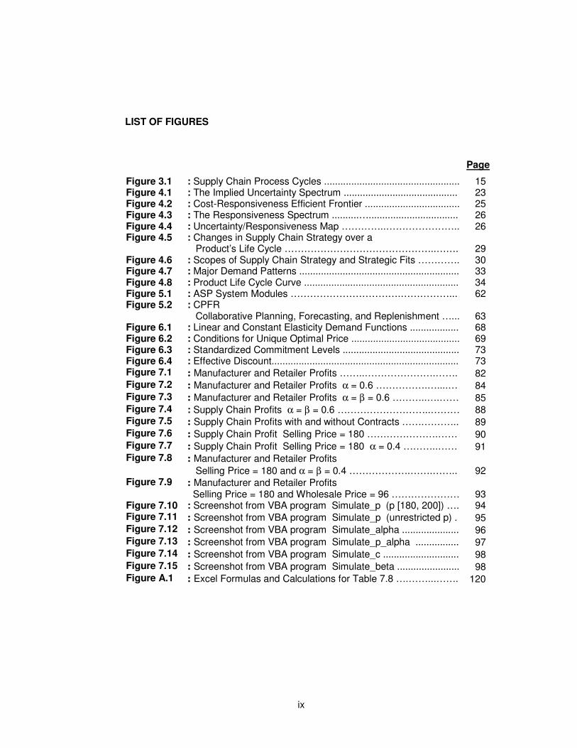
LIST OF FIGURES

Page

Figure 3.1 : Supply Chain Process Cycles .................................................. 15 Figure 4.1 : The Implied Uncertainty Spectrum .......................................... 23 Figure 4.2 : Cost-Responsiveness Efficient Frontier ................................... 25 Figure 4.3 : The Responsiveness Spectrum ..........…................................. 26 Figure 4.4 : Uncertainty/Responsiveness Map …………..………………….. 26 Figure 4.5 : Changes in Supply Chain Strategy over a

Product’s Life Cycle ………………………………………..……. 29 Figure 4.6 : Scopes of Supply Chain Strategy and Strategic Fits …………. 30 Figure 4.7 : Major Demand Patterns ........................................................... 33 Figure 4.8 Figure 5.1 Figure 5.2

: Product Life Cycle Curve ......................................................... : ASP System Modules …………………………….……………... : CPFR Collaborative Planning, Forecasting, and Replenishment …...

34 62 63

Figure 6.1 : Linear and Constant Elasticity Demand Functions .................. 68 Figure 6.2 : Conditions for Unique Optimal Price ........................................ 69 Figure 6.3 : Standardized Commitment Levels ........................................... 73 Figure 6.4 : Effective Discount..................................................................... 73 Figure 7.1 : Manufacturer and Retailer Profits ……..………………….……. 82 Figure 7.2 : Manufacturer and Retailer Profits α = 0.6 …………….…....… 84 Figure 7.3 : Manufacturer and Retailer Profits α = β = 0.6 ………..….…… 85 Figure 7.4 : Supply Chain Profits α = β = 0.6 ………………………..……… 88 Figure 7.5 : Supply Chain Profits with and without Contracts …….……….. 89 Figure 7.6 : Supply Chain Profit Selling Price = 180 ………………….…… 90 Figure 7.7 : Supply Chain Profit Selling Price = 180 α = 0.4 ………..…… 91 Figure 7.8 : Manufacturer and Retailer Profits

Selling Price = 180 and α = β = 0.4 ……………….…….…….. 92 Figure 7.9 : Manufacturer and Retailer Profits

Selling Price = 180 and Wholesale Price = 96 ………………… 93 Figure 7.10 : Screenshot from VBA program Simulate_p (p [180, 200]) …. 94 Figure 7.11 : Screenshot from VBA program Simulate_p (unrestricted p) . 95 Figure 7.12 : Screenshot from VBA program Simulate_alpha ..................... 96 Figure 7.13 : Screenshot from VBA program Simulate_p_alpha ................ 97 Figure 7.14 : Screenshot from VBA program Simulate_c ............................ 98 Figure 7.15 : Screenshot from VBA program Simulate_beta ....................... 98 Figure A.1 : Excel Formulas and Calculations for Table 7.8 ….……...……. 120

x

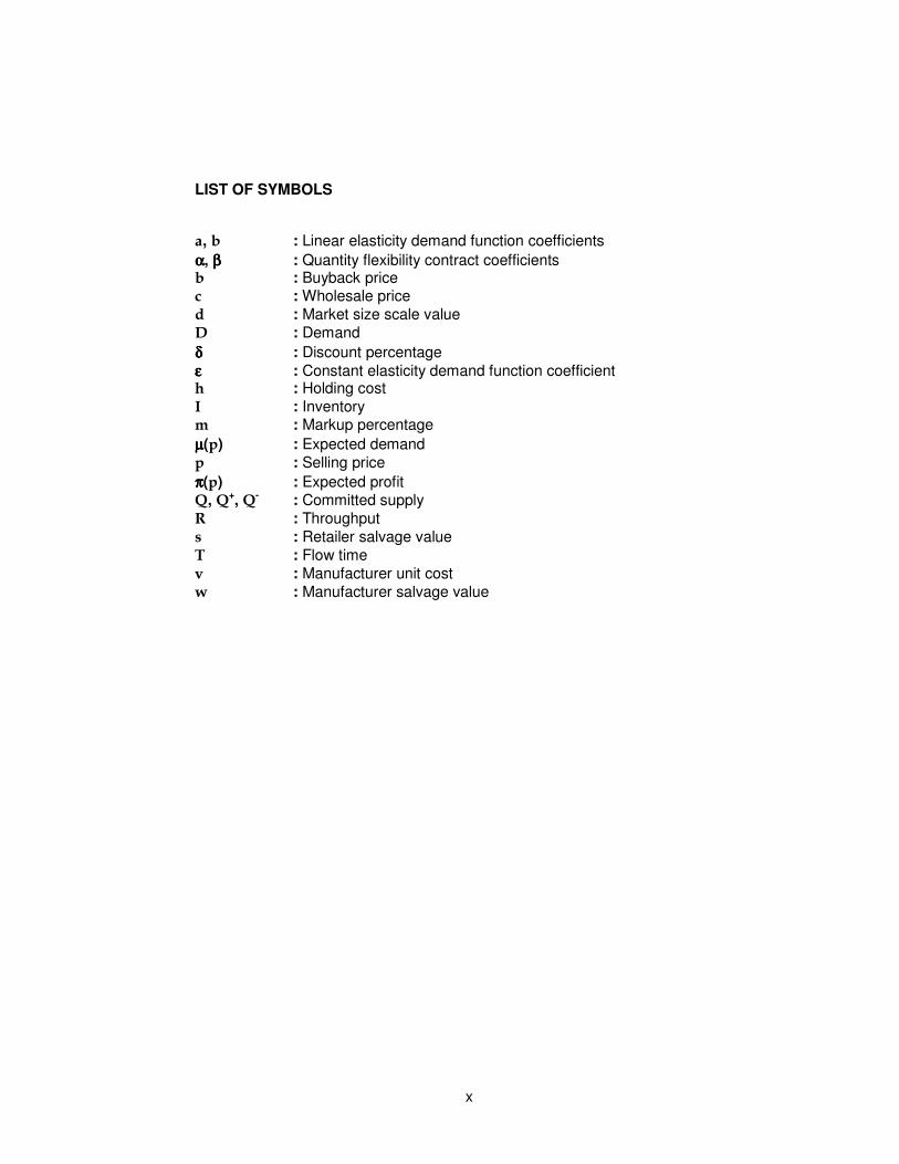
LIST OF SYMBOLS

a, b : Linear elasticity demand function coefficients αααα, ββββ : Quantity flexibility contract coefficients b : Buyback price c : Wholesale price d : Market size scale value D : Demand δδδδ : Discount percentage εεεε : Constant elasticity demand function coefficient h : Holding cost I : Inventory m : Markup percentage µµµµ(p) : Expected demand p : Selling price ππππ(p) : Expected profit Q, Q+, Q- : Committed supply R : Throughput s : Retailer salvage value T : Flow time v : Manufacturer unit cost w : Manufacturer salvage value

xi

A PRICE-SENSITIVE QUANTITY-FLEXIBLE SUPPLY CHAIN CONTRACT

MODEL AS A SUPPLY CHAIN PERFORMANCE DRIVER

SUMMARY

A supply chain consists of all stages involved, directly or indirectly, in fulfilling a

customer request. The objective of every supply chain is to maximize the overall

value generated. The value a supply chain generates is the difference between what

the final product is worth to the customer and the effort the supply chain expends in

filling the customer’s request. For most commercial supply chains, this value will be

strongly correlated with supply chain profitability, the difference between the

revenue generated from the customer and the overall cost across the supply chain.

The objective of maximizing this supply chain surplus can be achieved by improving

the supply chain performance in terms of efficiency and responsiveness using the

four supply chain drivers: inventory, transportation, facilities, and information.

In this dissertation, we discussed these four drivers and introduced supply chain

contracts as another driver to maximize supply chain profitability. Of particular

interest here are contracts that specify the parameters within which a buyer places

orders and a supplier fulfills them in order to maximize the total supply chain

surplus.

We discussed two supply chain contract models. First, where a retailer facing price

sensitive demand may obtain a discount by committing a fixed quantity over a finite

horizon, and second where a manufacturer offering buyback or quantity flexibility

contracts may increase the total supply chain profit.

We concluded that the first model incorporates demand as a function of the selling

price but does not address the crucial issue of total supply chain surplus

maximization. On the other hand, the second model, although it increases the total

supply chain surplus, does not incorporate the demand elasticity.

We then developed a model to address the individual weaknesses of the models

discussed by incorporating the price sensitive demand into quantity flexibility

contracts by determining the optimal level of product availability, as a function of the

xii

selling price, which maximizes the total supply chain profit. We also proposed two

solutions to the issue of profit sharing related to the distribution of the additional

supply chain profit generated by using the contracts. We then showed, through

numerical experiments, that our model maximizes total supply chain surplus by

incorporating demand elasticity and profit sharing into quantity flexibility contracts.

It is our belief that the supply chain contract model developed in this dissertation can

be an integral part of any Advanced Planning and Scheduling (APS) system.

xiii

FİYATA DUYARLI VE MİKTAR ESNEKLİĞİ OLAN BİR TEDARİK ZİNCİRİ

SÖZLEŞMESİ MODELİNİN TEDARİK ZİNCİRİ PERFORMANS GELİŞTİRİCİSİ

OLARAK KULLANIMI

ÖZET

Tedarik zinciri, bir ürünün tasarım aşamasından son müşterinin eline ulaşıncaya

kadar geçireceği ve gerekli olan tüm aşamaları kapsar. Her tedarik zincirinin amacı

kattığı değeri en üst düzeye çıkartmaktır. Bu değer tüketiciye ulaşan en son ürünün

getirisiyle tedarik zincirinin bu ürünü müşteriye ulaştırıncaya kadar harcadığı tüm

emeklerin arasındaki farktır. Genelde bütün ticari tedarik zincirlerinde bu katma

değer, tedarik zincirinin tüketiciden elde ettiği getiri ile ürünün toplam maliyeti

arasındaki farka eşittir. Bu katma değeri en üst düzeye çıkartma amacı tedarik

zincirinin etkinliğini arttırmakla, diğer bir deyişle, en az masraf ile tüketici

beklentilerini en üst düzeyde karşılamakla sağlanır. Bunun için de tedarik zincirinin

bilinen dört performans geliştiricisi: stok, nakliyat, tesisler, ve bilgi sistemleri

kullanılır.

Çalışmamızda, yukarıdaki dört performans geliştiricisi bu yönden incelenmiş ve

tedarik zinciri sözleşmelerinin bir diğer performans geliştiricisi olarak nasıl tedarik

zinciri katma değerini en üst düzeye çıkartmada kullanılabileceği araştırılmıştır.

Özellikle, tedarik zinciri içindeki bir üretici ve satıcı arasında tedarik zinciri katma

değerini en üst düzeye çıkaran fiyat ve miktarları belirleyen sözleşmeler

incelenmiştir.

İki tedarik zinciri sözleşmesi modeli incelenmiştir. İlk sözleşme tipi olarak, ürüne olan

talebin satış fiyatı ile bağlantılı olduğu bir ortamda, üreticinin satıcıya belli bir

miktarda ürün alma garantisi karşılığı önerdiği indirimler incelenmiştir. İkinci

sözleşme tipi olarak ise, üreticinin toplam tedarik zinciri katma değerini arttırmak için

satıcıya önerdiği satılamayan ürünü geri alma veya satın almada miktar esnekliği

sağlama sözleşmeleri ele alınmıştır.

Birinci modelde, görüleceği üzere, her ne kadar talep satış fiyatı ile bağlantılı ise de,

sonuç yalnız satıcı açısından değerlendirildiğinden, modelin tedarik zinciri toplam

xiv

katma değeri üzerindeki etkisi belirsizdir. Diğer yandan, ikinci model tedarik

zincirinin toplam katma değerini arttırdığı halde, talebin fiyat duyarlılığı göz önüne

alınmamıştır.

Çalışmamızda, bu modellerin zayıf noktalarına cevap veren ve talebin fiyata duyarlı

olduğu bir ortamda üretici-satıcı arasında miktar esnekliği sağlayarak tedarik zinciri

katma değerini en üst düzeye çıkaran bir model geliştirdik ve sözleşmeden

kaynaklanan bu ek katma değer artışının her iki tarafın da kazanması için nasıl

paylaştırılabileceğini gösteren iki yöntem belirledik. Ayrıca, geliştirdiğimiz fiyata

duyarlı olan ve ek katma değer artışının paylaşımını sağlayan miktar esnekliği

modelinin tedarik zinciri katma değerini en üst düzeye çıkarardığını sayısal

örneklerle gösterdik.

İnancımız, bu çalışmada geliştirilen tedarik zinciri sözleşme modellerinin bütün APS

(Advanced Planning and Scheduling / İleri Planlama ve Çizelgeleme) sistemlerinde

kullanılabileceğidir.

1

CHAPTER 1. INTRODUCTION

APICS, The Educational Society for Resource Management, dictionary defines the

term supply chain as the processes from the initial raw materials to the ultimate

consumption of the finished product linking across supplier-user companies [1, p: 3].

A supply chain consists of all stages involved, directly or indirectly, in fulfilling a

customer request. Over the last three decades, information technology resources,

such as Electronic Data Interchange (EDI), the Internet, Enterprise Resource

Planning (ERP), and Supply Chain Management (SCM) software have reshaped

how firms manage the production and distribution of goods and services by sharing

and analyzing the information in the supply chain. Competitive pressures have

forced the companies to streamline supply chain operations to increase their

efficiency while improving their responsiveness.

The supply chain performance in terms of efficiency and responsiveness can be

improved using the four supply chain drivers: inventory, transportation, facilities, and

information [2, p: 50]. The supply chain not only includes the manufacturer and

suppliers, but also transporters, warehouses, retailers, and customers themselves.

The forecast of future customer demand and its unavoidable variability form the

basis for all strategic and planning decisions in a supply chain in terms of production

and distribution.

In this dissertation, we present a series of models to redistribute the absorption of

variability using contracts and show that effective use of contracts as a supply chain

driver can substantially increase the overall supply chain profitability and its

competitive advantage by forcing companies to evaluate every action in the context

of the entire supply chain. A company’s partners in the supply chain may well

determine the company’s success, as the company is intimately tied to its supply

chain partners. This broad intercompany scope increases the size of the surplus to

be shared among all stages of the supply chain.

2

1.1 Supply Chain Contracts and Committed Delivery Strategies

A contract specifies the parameters within which a buyer places orders and a

supplier fulfills them. It may contain specifications regarding quantity, price, time,

and quality. At one extreme, a contract may require the buyer to specify the precise

quantity required, with a very long lead time. In this case, the buyer bears the risk of

overstocking and understocking, and the supplier has exact order information well

advance of delivery. At the other extreme, buyers may not be required to commit to

the precise purchase quantity until they are certain of their demand, with the supply

arriving with a short lead time. In this case, the supplier has little advance

information, and the buyer can wait until demand is known before ordering. As a

result, the supplier must build inventory in advance and bear most of the risk of

overstocking and understocking. As contracts change, the risk different stages of the

supply chain bear changes, which affects the retailer’s and supplier’s decisions and

the supply chain profitability.

In this dissertation, we will analyze three specific types of contracts:

• Committed deliveries where by committing to periodic deliveries of a specific

quantity, a retailer facing price-sensitive demand absorbs some of the

supply chain variability in exchange of a discount on committed deliveries.

• Buyback contracts where the manufacturer specifies a wholesale price

along with a buyback price at which the retailer can return any unsold units.

• Quantity flexibility contracts where the manufacturer allows the retailer to

change the quantity ordered after observing demand.

1.2 Overview

This dissertation examines several supply chain contracts. In Chapter 2, we review

relevant literature. In Chapter 3, we look at various supply chain stages, decision

phases, cycles, and supply chain implementation with the objective of maximizing

the overall value generated by the supply chain. In Chapter 4, we review the supply

chain performance in terms of a strategic fit to match supply chain’s responsiveness

with demand uncertainty along with major demand patterns, and the need of an

Intercompany Interfunctional scope to maximize total supply chain surplus. We also

look at various supply chain drivers to achieve the balance between efficiency and

3

responsiveness, and obstacles to achieve this strategic fit as well as the implications

of supply chain management in agile manufacturing.

In Chapter 5, we look at the impact of information technology structure upon the

development and rapid expansion of supply chain collaboration as we review

various enterprise execution systems. Particularly, In Section 5.3 we look at how

Advanced Planning and Scheduling (APS) systems seek to integrate information

and coordinate overall supply chain decisions while recognizing the dynamics

between functions and processes. In a sense, supply chain contracts we developed

also seek the same objective while recognizing the dynamics between supply chain

partners. Using Collaborative Planning, Forecasting, and Replenishment (CPFR)

processes, the necessary coordination can be achieved.

In Chapter 6, we present various contract models and then develop our own model.

Sections 6.1 and Section 6.2 describe Retailer Profit without and with Commitment

Opportunity, respectively, with Demand as a Function of the Selling Price. The

strength of the model is the inclusion of demand as a function of the selling price.

However, the model is restricted with the intracompany scope maximizing only the

retailer’s profit without taking into account the total supply chain profit. The same is

true for Retailer Profit without Commitment Opportunity with Normally Distributed

Demand described in Section 6.3.

Section 6.4 addresses the weakness of intracompany approach by introducing the

total supply chain surplus with the intercompany view, which requires that both the

manufacturer and the retailer evaluate their actions in the context of the entire

supply chain. Section 6.5 and Section 6.6 describe how to maximize the total supply

chain surplus using Buyback Contracts and Quantity Flexibility Contracts,

respectively, with Normally Distributed Demand. Both buyback and quantity flexibility

contracts help maximize the total supply chain profit. However, there are two issues

that need to be addressed. The first one is related to profit sharing, i.e., how to

share the additional supply chain surplus thus generated. The second issue, the

main weakness of the contracts discussed, is the fact that demand has not been

correlated to the selling price.

In Chapter 7, we introduce our proposed model. First, in Section 7.1, we analyze

and then evaluate two solutions to address the issue of profit sharing for quantity

flexibility contracts. Then in Section 7.2, we develop a model to address the

individual weaknesses of the models discussed by incorporating the price-sensitive

demand into quantity flexibility contracts to maximize the total supply chain profit:

4

Committed Deliveries using Quantity Flexibility Contracts to Maximize Supply Chain

Surplus with Demand as a Function of the Selling Price. In Section 7.3, we develop

a computer program to help simulate the system to find optimum contract

parameters. Finally, in Section 7.4, we compare the models and emphasize the

benefits of using supply chain contracts with a price-sensitive demand function and

profit sharing.

In Chapter 8, we summarize our findings and discuss areas for future research.

5

CHAPTER 2. LITERATURE REVIEW

There has been much research addressing coordination among stages in the supply

chain [3]. The literature covering supply chain management is vast and well

developed. However, In spite of their prevalence in industry over the last thirty

years, little has appeared in Operations Research or Management Science literature

discussing supply chain contracts. Historically, the business literature has extolled

the virtues of using multiple suppliers as a means of improving negotiating position.

Heide [4] provides a review of existing theories of relationship management from a

marketing channel perspective. Ellinger [5] and Hagy [6] emphasize the importance

of integration and point to the need of a strong and significant relationship within the

supply chain.

Noordewier, John, and Nevin [7] set forth a theory that stronger interorganizational

ties result in greater adaptive capabilities, thus firms with closer ties are better able

to react to variability. Buvik and John [8] expand this theory to include the

implications of asset specificity. Cashon and Fisher [9] support the notion of all

players working as a unit focused on the requirements of product development and

the value of shared information.

Chandra and Kumar [10] analyze various issues important to supply chain

management and provide broader awareness of supply chain principles and

concepts. Balloe, Gilbert, and Mukherjee [11] discuss the new managerial

challenges from supply chain opportunities. Motwani, Larsin, and Ahuja [12] present

a survey of the global supply chain management (GSCM) literature with specific

emphasis on the application of the process, services and products used by

organizations to achieve competitive advantage and market position.

Fox, Chionglo, and Barbuceanu [13] describe the goals and architecture of the

Integrated Supply Chain Management System (ISCM). They consider the supply

chain as a system which can be managed by a set of intelligent software agents,

each responsible for one or more activities in the supply chain, and each interacting

with other agents in the planning and execution of their responsibilities.

6

Sengupta and Turnbull [14] review the general ideas of supply chain, the key point

being to keep all units synchronized and to solve the entire business problem by

manoeuvring through upstream and downstream information. Success of the supply

chain depends on several primary factors, including early visibility to changes in

demand all along the supply chain and a single set of plans that drives the supply

chain and integrates information.

Humphreys, Shiu, and Chan [15] present the initial findings from the responses of

large companies in Hong Kong and show the trend in supply chain relationships

moving towards a more collaborative approach. Tracey and Tan [16] discuss a

confirmatory factor analysis and path analysis to examine empirically the

relationships among supply chain partners, and Masella and Rangone [17] propose

different vendor selection systems based on the cooperative relationships. Liu, Ding,

and Lall [18] demonstrate an application of data envelopment analysis in evaluating

the relationships on the overall performance of suppliers in a manufacturing firm.

Weber, Current, and Desai [19] present a similar approach using data envelopment

analysis and multi objective programming.

Lambert, Cooper, and Pagh [20] provide several approaches to define supply chain

and its complexity. Trent and Monczka [21] discuss the complexity of external

organizational systems and difficulties in fostering close partnerships and integration

across the supply chain. Milgate [22] presents a conceptual model to identify basic

dimensions of the complexity involved. Spina and Zotteri [23] explore strategic and

structural contingencies surrounding partnerships in a global survey and analyze

collaborative practices along the operations integration and co-design dimensions.

Anupindi and Akella [24] develop optimal ordering policies for a single buyer with

multiple vendors. They present an optimal ordering policy that orders nothing when

the inventory level is above an upper bound, orders from one vendor when the

inventory level is between bounds, and orders from both vendors when the inventory

level is below the lower bound.

Kohli and Park [25] investigate joint ordering policies as a method to reduce costs

between a single vendor and a group of buyers. They present expressions for

optimal joint order quantities assuming all products are ordered in each joint order.

Their model calculates the savings in fixed order costs, but does not explicitly model

transportation costs. Furthermore, the requirement that every product is included in

each order is limiting.

7

He et. al. [26] examine the effect of order crossing in a system with stochastic lead

times. They show that the common single cycle analysis approach overestimates

both cost and optimal order quantity.

Weng [27-29] addresses a two-echelon, infinite horizon model with quantity

discounts and price-sensitive demand. His work focuses on using quantity discount

schedules as a mechanism for channel coordination. Rau, Wu, and Wee [30]

present an integrated inventory model under a multi-echelon supply chain

environment.

Building on a work of Ernst and Pyke [31] and Yano and Gerchak [32], Henig et. al.

[33] study a two-echelon system where a discount is offered for transportation

capacity commitment. For an infinite horizon, stationary demand system, they show

that for a given level of contracted transportation capacity, the optimal ordering

policy is characterized by two critical numbers such that when on-hand inventory

falls within a certain range, exactly the contracted capacity is used.

Bassok and Anupindi [34] develop optimal inventory policies for a firm that has

made a quantity commitment over some finite horizon. In their model, the

committing firm is free to order any quantity in any period, as long as the total

contracted quantity is purchased by the end of the horizon.

Anupindi and Bassok [35] develop approximations for an inventory system with

multiple items and a discount for a total volume commitment. The supplier extends

the discount to a certain fraction above the commitment level. In numerical studies,

they observe that increased demand variability leads to increased commitment, and

increased flexibility offered by the supplier leads to decreased commitment.

Bassok et. al. [36] study a finite horizon, stochastic demand inventory system with a

supply contract frequently used in the electronic component industry. The contract

requires the buyer to commit to order quantities in each of T periods. In the current

period, the buyer must order a quantity within a fixed percentage α of the committed

quantity. The buyer may also update future period commitments within a fixed

percentage β.

Eppen and Iyer [37, 38] examine a two-stage stochastic inventory model. Their

model is motivated by backup agreements common to the fashion industry. Under

such an agreement, a buyer chooses an order quantity, and the vendor holds back a

fraction of the commitment. After observing initial demand, the buyer can acquire up

8

to the remainder of their commitment at the original price, paying a penalty cost for

committed units not purchased.

Tsay [39] models a manufacturer-retailer chain where the retailer gives a point

estimate of demand. The two parties then agree on a minimum purchase

commitment, a maximum quantity guaranteed to be available, and a transfer price.

He shows that without such contract structure, inefficiencies may result.

Vargas and Metters [40] present a dual-buffer approach designed to improve the

cost and fill rate performance of a production system. They apply basic lot-sizing

techniques to demand forecasts and use stochastic inventory theory to set safety

stock levels. Their approach attempts to avoid scheduling a replenishment order

merely to replenish safety stock.

Smith and Zhang [41] study infinite horizon production planning with convex

production and inventory costs and time varying, deterministic demand. They show

that the optimal production levels for the infinite horizon problem can be obtained by

solving a series of finite horizon problems. They also derive expressions for the

minimum horizon length.

DeCroix and Arreola-Risa [42] examine an inventory system where the likelihood

that demand is lost rather than backlogged can be influenced by an economic

incentive. They assume a backorder response function to describe the probability

that customers will agree to backorder as a function of a monetary incentive offered.

Optimal control parameters and backorder incentives can be found efficiently when

the decision to offer the incentive can be made when a shortage occurs.

Glasserman and Tayur [43] present a computational method for estimating inventory

cost sensitivity with respect to centralized system parameters for a capacitated

serial inventory system. Lee and Whang [44] reconsidered the same serial inventory

system where operational decisions are made locally. The incentive scheme

proposed requires all stages to share both demand distribution and cost parameters

information. Ganeshan, Boone, and Stenger [45] study the impact of inventory and

flow planning parameters on supply chain performance.

Kapuscinksi and Tayur [46] study a capacitated production-inventory model with

seasonal demand. They establish that the optimal policy takes the form of a

modified order-up-to system where the producer builds up to the order-up-to level,

or as close to this level as possible if bounded by capacity. Excess demand is

9

backlogged. Results from numerical experimentation indicate that increased mean

demand, increased demand variability, and decreased capacity all lead to increased

order-up-to levels. Zipkin [47] addresses the uncapacitated version of this problem.

Moon, Kim, and Hur [48] study an integrated process planning and scheduling to

minimize total tardiness in a multi-plants supply chain and Tipme and Kallrath [49]

present an optimal planning in large multi-site production networks. Vergara,

Khouja, and Michalewicz [50] discuss an algorithm optimizing material flow order

release and Chan et. al. [51] develop a simulation model to assess order release

mechanisms. Syarif, Yun, and Gen [52] also study a multi-stage logistics chain

network and present a spanning tree-based generic algorithm.

Doran [53] discusses a case study examining the characteristics of synchronous

manufacturing within an automotive context and concludes that the nature of buyer-

supplier relationships moves toward a modular supply model. Min and Guo [54]

develop a cooperative competition strategy in line with the modular supply model

and Han et. al. [55] present a similar model for supply chain integration in

developing countries.

Masters [56] examines multi-echelon distribution inventories and develops a model

determining near optimal stock levels. Sox and Muckstadt [57] study a multi-item,

multi-period production planning problem with stochastic demand. They develop a

Lagrangian relaxation algorithm that performs quite well in numerical experiments.

Moinzadeh and Nahmias [58] develop a continuous review, stochastic demand

inventory with two supply modes. Lead times are deterministic. One of the modes

has a shorter lead time and is more expensive either in fixed order cost, variable

cost, or both. This faster mode is used as an emergency mode. The form of the

policy they analyze is a generalization of the well known (Q, R) policy, where an

order Q1 units is placed via the slower mode when on-hand inventory drops to R1. If

on-hand inventory drops to R2, and an order placed via the fast method will arrive

before the outstanding order for Q1 arrives, an order for Q2 is placed. Numerical

experiments indicate that substantial savings can be obtained by using two modes.

Gurnani [59] studies a stochastic demand, finite horizon, periodic review inventory

system where the probability that the supplier offers a discounted price in any time

period is some constant β. In each period, the distributor chooses an order quantity

at the regular price before learning if there will be a discount offered. The optimal

10

policy is defined by three regions. If inventory is above a high threshold value, order

nothing, even if a discount is offered. If inventory is below the high threshold but

above a lower one, it is optimal to order if a discount is offered. If inventory is below

the low threshold value, it is optimal to order even at full price.

Zheng [60] analyzes a continuous review model with stochastic demand and

discount opportunities arriving according to a Poisson process. The author

establishes that a two-tiered reorder point model (s, c, S) is optimal. That is, when

on-hand inventory drops to s, order up to S. When a discount opportunity arrives, if

inventory is below c, order up to S.

Moinzadeh [61] studies a continuous review, deterministic demand model with

discount opportunities that arrive according to a Poisson process. The optimal policy

takes on a two-tiered form, similar to that in Zheng [60].

Ritchken and Tapiero [62] consider a risk management approach using negotiated

option contracts for hedging against quality and price uncertainty in the procurement

of inventory. They design an optimal mesh of contingent claims with purchasing

commitments that will best meet the risk-reward preferences of the decision maker.

Kohli and Park [63] take a game theoretical approach to the problem of deterministic

inventory acquisition. They consider quantity discounts, which are offered by a

monopolistic supplier in the context of a bargaining problem where the buyer and

supplier negotiate over the average unit price and the order quantity. They consider

both incremental and block discounts in the model and show that the outcome of the

negotiations maximizes the joint efficiency gain between the buyer and the supplier.

Gallego and Moon [64] analyze the newsvendor problem with normally distributed

price-sensitive demand. Numerous extensions to the newsvendor problem have

been proposed in the academic literature.

Lau and Lau [65] introduce a price-sensitive demand model under two objectives:

maximize expected profit, and maximize the probability of achieving a target level of

profit.

Khouja [66] examines a newsvendor model where a fixed proportion of excess

demand can be satisfied from an emergency supply option. Two objective functions

are examined: maximize expected profit and maximize probability of achieving a

target profit.

11

Thomas [67] develops a model for a distributor facing price-sensitive demand and

given the opportunity to receive a discount on fixed quantity committed deliveries.

He also analyzes the pricing and profit implications of committed delivery strategies

and extends his model to committed deliveries with flexible quantities. Using

computational experiments, he shows that the value of flexibility in commitments is

significant, especially when the commitment discount is relatively large compared to

the holding cost. Using a constant elasticity expected demand function, simple

expressions capturing price and profit sensitivity are developed.

Barnes-Schuster [68] discusses how the long term contracts influence the activities

of a buyer-supplier relationship. The author shows that system safety stocks should

not be split between a buyer and supplier and derives conditions indicating when the

supplier or the buyer(s) should keep the system safety stock based on system cost

parameters, production lead times, and demand distributions.

12

CHAPTER 3. SUPPLY CHAIN MANAGEMENT

A supply chain consists of all stages involved, directly or indirectly, in fulfilling a

customer request. The supply chain not only includes the manufacturer and

suppliers, but also transporters, warehouses, retailers, and customers themselves.

Within each organization, such as a manufacturer, the supply chain includes all

functions involved in filling a customer request. These functions include, but not

limited to, new product development, marketing, operations, distribution, finance,

and customer service [2, p: 3-15].

A supply chain is dynamic and involves the constant flow of information, product,

and funds between different stages. Each stage of the supply chain performs

different processes and interacts with other stages of the supply chain. The primary

purpose for the existence of any supply chain is to satisfy customer needs, in the

process generating profits for itself. Supply chain activities begin with a customer

order and end when a satisfied customer has paid for the purchase. It is important to

visualize information, product, and funds flows along both directions of this chain

and it may be more accurate to use the terms supply network or supply web to

describe the structure of a supply chain [69-73].

Although each stage need not be present, a typical supply chain includes:

• Suppliers

• Manufacturers

• Distributors

• Retailers

• Customers

The objective of every supply chain is to maximize the overall value generated. The

value a supply chain generates is the difference between what the final product is

worth to the customer and the effort the supply chain expends in filling the

customer’s request. For most commercial supply chains, value will be strongly

correlated with supply chain profitability, the difference between the revenue

generated from the customer and the overall cost across the supply chain.

13

All flows of information, product, and funds generate costs within the supply chain.

Supply Chain Management (SCM) involves the management of flows between and

among stages in a supply chain to maximize total profitability.

3.1 Decision Phases in a Supply Chain

Successful supply chain management requires several decisions relating to the flow

of information, product, and funds. These decisions fall into three categories or

phases, depending on the frequency of each decision and the time frame over which

a decision phase has an impact: strategy, planning, and operation phases.

3.1.1 Supply Chain Strategy

During this phase, a company decides how to structure the supply chain. It decides

what the chain’s configuration will be and what processes each stage will perform.

Strategic decisions made by companies include the location and capacities of

production and warehousing facilities, products to be manufactured or stored at

various locations, modes of transportation to be made available along different

shipping legs, and type of information system to be utilized. A company must ensure

that the supply chain configuration supports its strategic objectives during this

phase. Strategic supply chain decisions are typically made for the long term and are

very expensive to alter on short notice. Consequently, when companies make these

decisions, they must take into account uncertainty in anticipated market conditions

over the next few years.

3.1.2 Supply Chain Planning

During this phase, companies define a set of operating policies that govern short

term operations based on the supply chain’s configuration determined in the

strategic phase that establishes constraints within which planning must be done.

Typically, companies start the planning phase with a forecast for the coming year of

demand in different markets. Planning includes decisions regarding which markets

will be supplied from which locations, the planned build-up of inventories, the

subcontracting of manufacturing, the replenishment and inventory policies to be

followed, the policies that will be enacted regarding backup locations in case of a

stockout, and the timing and size of marketing promotions. Planning establishes

parameters within which a supply chain will function over a specified period of time.

14

In the planning phase, companies must include uncertainty in demand, exchange

rates where applicable, and competition over the time horizon in their decisions.

3.1.3 Supply Chain Operation

During this phase where the time horizon is weekly or daily, companies make

decisions regarding individual customer orders. At the operational level, supply

chain configuration is considered fixed and planning policies defined. The goal of

supply chain operations is to implement the operating policies in the best possible

manner. The companies allocate individual orders to inventory or production, set a

date that an order is to be filled, generate pick lists at a warehouse, allocate an

order to a particular shipping mode and shipment, set delivery schedules, and place

replenishment orders. Because operational decisions are being made in the short

term, there is less uncertainty about demand information. The goal during this phase

is to exploit the reduction of uncertainty and optimize performance within the

constraints established by the configuration and planning policies.

3.2 Process View of a Supply Chain

A supply chain is a sequence of processes and flows that take place within and

between different supply chain stages and combine to fill a customer need for a

product. There are two different ways to view the processes performed in a supply

chain: Cycle view and Push/Pull view.

3.2.1 Cycle View

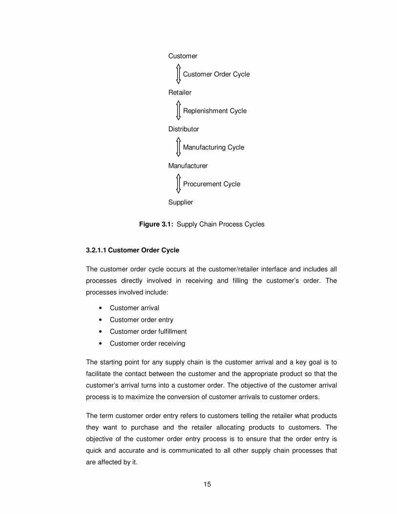
The processes in a supply chain are divided into a series of cycles, each performed

at the interface between two successive stages of a supply chain. Given the five

stages of a supply chain, all supply chain processes can be broken down into four

process cycles as shown in Figure 3.1 [2, p: 8].

15

3.2.1.1 Customer Order Cycle

The customer order cycle occurs at the customer/retailer interface and includes all

processes directly involved in receiving and filling the customer’s order. The

processes involved include:

• Customer arrival

• Customer order entry

• Customer order fulfillment

• Customer order receiving

The starting point for any supply chain is the customer arrival and a key goal is to

facilitate the contact between the customer and the appropriate product so that the

customer’s arrival turns into a customer order. The objective of the customer arrival

process is to maximize the conversion of customer arrivals to customer orders.

The term customer order entry refers to customers telling the retailer what products

they want to purchase and the retailer allocating products to customers. The

objective of the customer order entry process is to ensure that the order entry is

quick and accurate and is communicated to all other supply chain processes that

are affected by it.

Customer

Retailer

Distributor

Manufacturer

Supplier

Customer Order Cycle

Replenishment Cycle

Manufacturing Cycle

Procurement Cycle

Figure 3.1: Supply Chain Process Cycles

16

During the customer order fulfillment process, the customer’s order is filled and sent

to the customer. All inventories will need to be updated, which may result in the

initiation of the replenishment cycle. In general, customer order fulfillment takes

place from retailer inventory. In a build-to-order scenario, in contrast, order

fulfillment takes place directly from the manufacturer’s production line. The objective

of the customer order fulfillment process is to get the correct and complete orders to

customers by the promised due dates and at the lowest possible cost.

During the customer order receiving process, the customer receives the order and

takes the ownership. Records of this receipt may be updated and payment initiated.

3.2.1.2 Replenishment Cycle

The replenishment cycle occurs at the retailer/distributor interface and includes all

processes involved in replenishing retailer inventory. It is initiated when a retailer

places an order to replenish inventories to meet future demand. The replenishment

cycle is similar to the customer order cycle except that the retailer is now the

customer. The objective of the replenishment cycle is to replenish inventories at the

retailer at minimum cost while providing the necessary product availability to the

customer. The processes involved include:

• Retail order trigger

• Retail order entry

• Retail order fulfillment

• Retail order receiving

As the retailer fills customer demand, inventory is depleted and must be replenished

to meet future demand. A key activity the retailer performs during replenishment

cycle is to devise replenishment or ordering policy that triggers an order. The

objective when setting replenishment order triggers is to maximize profitability by

balancing product availability and cost. The outcome of the retail order trigger

process is that a replenishment order is generated.

The retail order entry process is similar to customer order entry at the retailer. The

only difference is that the retailer is now the customer placing the order with the

distributor or manufacturer. The objective of the retail order entry process is that an

order be entered accurately and conveyed quickly to all supply chain processes

affected by the order.

17

The retail order fulfillment process is very similar to customer order fulfillment except

that it takes place either at the distributor or the manufacturer. A key difference is

the size of each order. Customer orders tend to be much smaller than replenishment

orders. The objective of the retail order fulfillment is to get the replenishment order

to the retailer on time while minimizing costs.

Once the replenishment order arrives at a retailer, the retailer must receive it

physically, update all inventory records, and settle all payable accounts. The

process involves product flow from the distributor or the manufacturer to the retailer

as well as information and financial flows. The objective of the retail order process is

to update inventories and displays quickly and accurately at the lowest possible

cost.

3.2.1.3 Manufacturing Cycle

The manufacturing cycle typically occurs at the distributor/manufacturer (or retailer/

manufacturer) interface and includes all processes involved in replenishing

distributor (or retailer) inventory. The manufacturing cycle is triggered by customer

orders, replenishment orders from a retailer or distributor, or by the forecast of

customer demand and current product availability in the manufacturer’s finished

product warehouse. In general, a manufacturer produces several products and fills

demand from several sources. The manufacturing cycle can be reacting to customer

demand (referred to as a pull process) or anticipating customer demand (referred to

as a push process). The processes involved in the manufacturing cycle include:

• Order arrival from the distributor, retailer, or customer

• Production scheduling

• Manufacturing and shipping

• Receiving at the distributor, retailer, or customer

During the order arrival process, a distributor sets a replenishment order trigger

based on the forecast of future demand and current product inventories. The

resulting order is then conveyed to the manufacturer. In some cases, the customer

or the retailer may be ordering directly from the manufacturer. In other cases, a

manufacturer may be producing to stock a finished product warehouse. In the latter

situation, the order is triggered based on product availability and a forecast of future

demand. This process is similar to the retail order trigger process in the

replenishment cycle.

18

The production scheduling process is similar to the order entry process in the

replenishment cycle where inventory is allocated to an order. During the production

scheduling process, orders are allocated to a production plan or schedule. Given the

desired production quantities, the manufacturer must decide on the precise

production sequence. The manufacturer must also decide which products to allocate

each line if there are multiple production lines. The objective of the production

scheduling process is to maximize the proportion of orders filled on time while

keeping costs down.

The manufacturing and shipping process is equivalent to the order fulfillment

process in the replenishment cycle. During the manufacturing phase of the process,

the manufacturer produces to the production schedule while meeting quality

requirements. During the shipping phase of this process, the product is shipped to

the customer, retailer, distributor, or finished product warehouse. The objective of

the manufacturing and shipping process is to ship the product by the promised due

date while meeting quality requirements and keeping costs down.

In the receiving process, the product is received at the distributor, finished goods

warehouse, retailer, or customer, and inventory records are updated. Other

processes related to storage and fund transfers also take place.

3.2.1.4 Procurement Cycle

The procurement cycle occurs at the manufacturer/supplier interface and includes

all processes necessary to ensure that materials are available for manufacturing to

occur according to schedule. During the procurement cycle, the manufacturer orders

components from suppliers that replenish the component inventories. The

relationship is quite similar to that between a distributor and manufacturer, with one

significant difference: whereas retailer/distributor orders are triggered by uncertain

customer demand, component orders can be determined precisely once the

manufacturer has decided what the production schedule will be. Component orders

are dependent on the production schedule. Thus, it is important that suppliers be

linked to the manufacturer’s production schedule. However, if a supplier’s lead times

are long, the supplier has to produce to forecast because the manufacturer’s

production schedule may not be fixed that far in advance.

In practice, there may be several tiers of suppliers, each producing a component for

the next tier. A similar cycle would then flow back one stage to the next.

19

As a summary, the cycle view of the supply chain clearly defines the processes

involved and the owners of each process. This view is very useful when considering

operational decisions because it specifies the roles and responsibilities of each

member of the supply chain and the desired outcome for each process.

3.2.2 Push/Pull View

All processes in a supply chain fall into one of two categories, depending on the

timing of their execution relative to customer demand. In pull processes, execution is

initiated in response to a customer order. Push processes are those that are

executed in anticipation of customer orders. At the time of execution of a pull

process, demand is known with certainty. At the time of execution of a push

process, demand is not known and must be forecast. Pull processes may also be

referred to as reactive processes because they react to customer demand. Push

processes may also be referred to as speculative processes because they respond

to forecast rather than actual demand. The push/pull boundary in a supply chain

separates push processes from pull processes.

A push/pull view of the supply chain is very useful when considering strategic

decisions relating to supply chain design. This view forces a more global

consideration of supply chain processes as they relate to a customer order. Such a

view may result in responsibility for certain processes being passed on to a different

stage of the supply chain if making this transfer allows a push process to become a

pull process. Supply chain contracts help achieve these transfers.

3.3 How to Implement Supply Chain Management

The power of supply chain management is its potential to include the customer as a

partner in supplying the goods or services provided by a supply chain. Integration

improves the flow of information throughout the supply chain. Customer information

is more than data. It is data that has been analyzed in some manner so that there is

insight into the needs of the customer. In the typical supply chain the further the

members of a chain are from the end customer, the less understanding these

members have of the needs of the customer. This increases the supply chain

member’s uncertainty and complicates the planning. Firms respond to uncertainty

differently. Some firms may increase inventory while others may increase lead

times. Either action reduces their ability to respond to their customers. As

20

uncertainty is reduced because they have more information, firms are able to

develop plans with shorter lead times. By improving the information flow in the

supply chain, firms throughout the chain have less uncertainty to resolve during the

planning process. This, in turn, allows the chain to increase its responsiveness to

their customers [1, p: 5-10].

Another advantage of integrating the customer into the supply chain is that it

integrates the product development function with the other functions in the firm. This

integration allows the product development staff to communicate more with the

customer both internally and externally to the firm, which increases the firm’s

responsiveness to the customer’s needs.

Some firms use the concept of internal customer to remind their employees that

each employee performs just one step in a supply chain whose purpose is to

provide a good or service to the end customer. The purpose of the internal customer

logic is to keep each employee focused on the needs of the end customer. This

helps employees to recognize that not only is their firm just one link of a larger

supply chain, but that the firm itself can be viewed as a chain of processes each of

which is a customer of the preceding process.

Supply chain management requires an unprecedented level of cooperation between

the members of the supply chain. It requires an open sharing of information so that

all members know they are receiving their full share of the profits. Since many of the

firms in a supply chain may not have a history of cooperation, achieving the trust

necessary for supply chain management is a crucial task.

A firm in the supply chain must initiate the attempt to form partnerships and actively

manage the supply chain. Often a firm that has a large amount of market power in

the chain will become the leader of the supply chain.

This leader firm needs to justify the effort to manage the supply chain by explaining

the benefits that will accrue to each member in the supply chain and to itself. To do

this, the supply chain leader must show the partners where the improvements in the

supply chain will arise, and then how these improvements will lead to a gain for

everyone involved. To establish trust among the members of the supply chain, the

lead firm must also suggest how communication can be opened up and how every

member will be ensured that it is receiving its fair share of profits.

21

Managing a supply chain is more complex and difficult than managing an individual

firm. But, the principles of management used to integrate a firm’s own internal

functions also apply to managing the entire supply chain. For example, a well

understood phenomenon in the management of a firm is that there is always a

bottleneck that constrains sales. This bottleneck may be internal to the firm (a

process that cannot produce enough to meet demands) or it may be external to the

firm (market demand that is less than the capacity of the firm). This principle applies

to the entire supply chain. While the supply chain is driven by customer demand, it is

constrained by its own internal resources. One difference is that these resources

may not be owned by the same firm. It is possible for the output of an entire supply

chain to be limited because one firm does not have the capacity to meet the surging

demand. It is also possible for every firm in the supply chain to be operating at a low

utilization because there is not enough demand in the market for the products from

the supply chain. There are bottlenecks inside the supply chain just as there are

bottlenecks inside firms. To properly manage the supply chain, its members must be

aware of the location of their bottlenecks internally and also of the bottlenecks in the

entire supply chain.

22

CHAPTER 4. SUPPLY CHAIN PERFORMACE

Creating a strategic fit between a company’s competitive strategy and its supply

chain strategy affects performance. The intercompany scope of strategic fit requires

firms to evaluate every action in the context of the entire supply chain. This broad

scope increases the size of the surplus to be shared among all stages of the supply

chain. Achieving strategic fit is critical to a company’s overall success [2, p: 25-46].

4.1 Competitive and Supply Chain Strategies

A company’s competitive strategy defines the set of customer needs that it seeks to

satisfy through its products and services. To execute a company’s competitive

strategy, all the functions in its value chain play a role, and each must develop its

own strategy. In an organization, the value chain consists of new product

development, marketing and sales, operations, distribution, and service. It

emphasizes the close relationship between all the functional strategies within a

company. Each function is crucial if a company is to be profitably satisfying

customer needs. Therefore, the various functional strategies cannot be formulated in

isolation. They are closely intertwined and must fit and support each other if a

company is to succeed. A company’s competitive strategy and its supply chain

strategy must fit together.

4.2 Strategic Fit

Strategic fit means that both the competitive and supply chain strategies have the

same goal. It refers to consistency between the customer priorities that the

competitive strategy is designed to satisfy and the supply chain capabilities that the

supply chain strategy aims to build. There are three basic steps to achieving this

strategic fit: understanding the customer, understanding the supply chain, and

achieving strategic fit [2, 74-78].

23

4.2.1 Understanding the Customer

To understand the customer, a company must identify the needs of the customer

segment being served. In general, customer demand from different segments may

vary along several attributes:

• The quantity of the product needed in each lot

• The response time that customers are willing to tolerate

• The variety of products needed

• The service level required

• The price of the product

• The desired rate of innovation in the product

Each customer in a particular segment will tend to have similar needs, whereas

customers in different segments can have very different needs. In a very

fundamental sense, each customer need can be translated into the metric of implied

demand uncertainty, the uncertainty that exists due to the portion of demand that the

supply chain is required to meet. This is different than the demand uncertainty,

which reflects the uncertainty of customer demand for a product. For example, a firm

supplying only emergency orders for a product will face a higher implied demand

uncertainty than a firm that supplies the same product with a long lead time. Another

illustration of the need for this distinction is the impact of service level. As a supply

chain raises its service level, it must be able to meet a higher and higher percentage

of actual demand, forcing it to prepare for rare surges in demand. Thus, raising the

service level increases the implied demand uncertainty even though the product’s

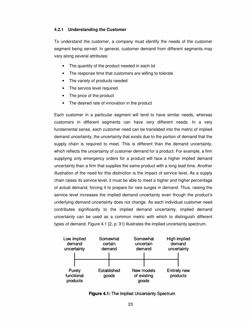
underlying demand uncertainty does not change. As each individual customer need

contributes significantly to the implied demand uncertainty, implied demand

uncertainty can be used as a common metric with which to distinguish different

types of demand. Figure 4.1 [2, p: 31] illustrates the implied uncertainty spectrum.

Figure 4.1: The Implied Uncertainty Spectrum

Low implieddemand

uncertainty

Somewhatcertain

demand

Somewhatuncertaindemand

High implieddemand

uncertainty

Purelyfunctionalproducts

Establishedgoods

New modelsof existing

goods

Entirely newproducts

Figure 4.1: The Implied Uncertainty Spectrum

Low implieddemand

uncertainty

Somewhatcertain

demand

Somewhatuncertaindemand

High implieddemand

uncertainty

Purelyfunctionalproducts

Establishedgoods

New modelsof existing

goods

Entirely newproducts

24

The first step in achieving strategic fit is to understand customers by mapping where

their demand is located on the implied uncertainty spectrum.

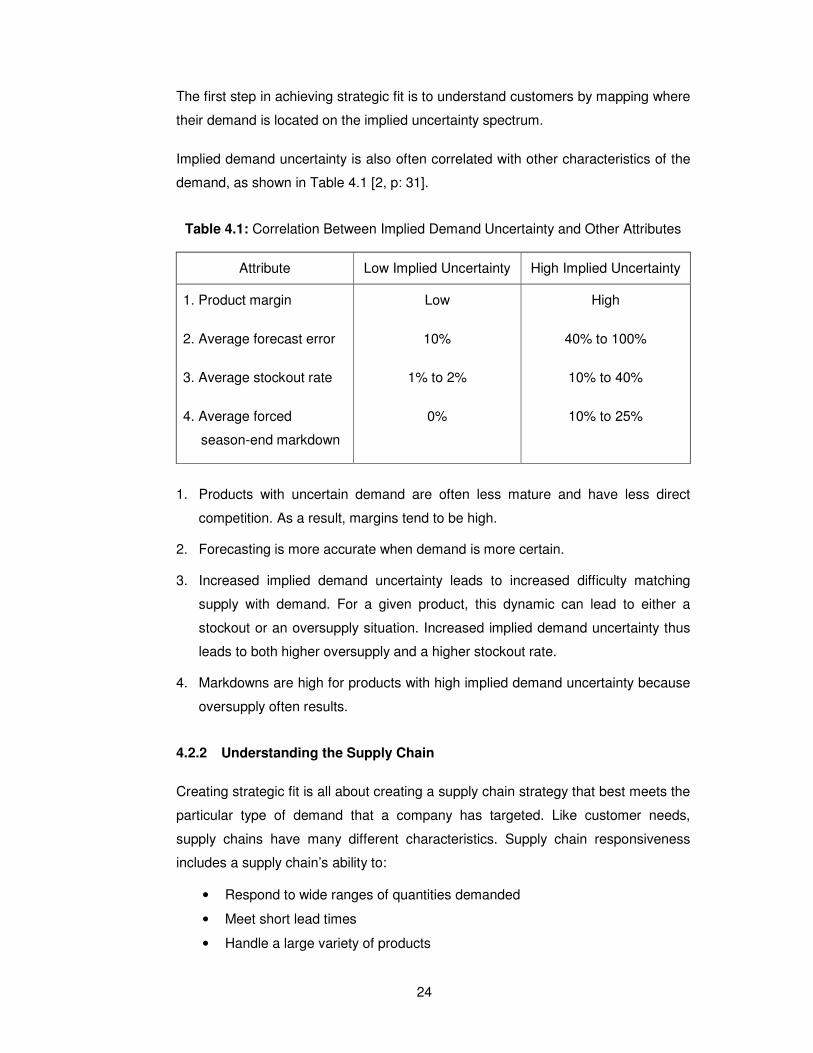
Implied demand uncertainty is also often correlated with other characteristics of the

demand, as shown in Table 4.1 [2, p: 31].

Table 4.1: Correlation Between Implied Demand Uncertainty and Other Attributes

Attribute Low Implied Uncertainty High Implied Uncertainty

1. Product margin

2. Average forecast error

3. Average stockout rate

4. Average forced

season-end markdown

Low

10%

1% to 2%

0%

High

40% to 100%

10% to 40%

10% to 25%

1. Products with uncertain demand are often less mature and have less direct

competition. As a result, margins tend to be high.

2. Forecasting is more accurate when demand is more certain.

3. Increased implied demand uncertainty leads to increased difficulty matching

supply with demand. For a given product, this dynamic can lead to either a

stockout or an oversupply situation. Increased implied demand uncertainty thus

leads to both higher oversupply and a higher stockout rate.

4. Markdowns are high for products with high implied demand uncertainty because

oversupply often results.

4.2.2 Understanding the Supply Chain

Creating strategic fit is all about creating a supply chain strategy that best meets the

particular type of demand that a company has targeted. Like customer needs,

supply chains have many different characteristics. Supply chain responsiveness

includes a supply chain’s ability to:

• Respond to wide ranges of quantities demanded

• Meet short lead times

• Handle a large variety of products

25

• Build highly innovative products

• Meet a very high service level

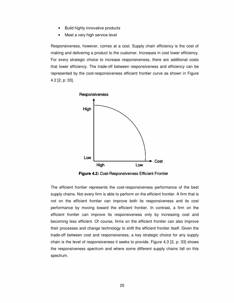
Responsiveness, however, comes at a cost. Supply chain efficiency is the cost of

making and delivering a product to the customer. Increases in cost lower efficiency.

For every strategic choice to increase responsiveness, there are additional costs

that lower efficiency. The trade-off between responsiveness and efficiency can be

represented by the cost-responsiveness efficient frontier curve as shown in Figure

4.2 [2, p: 33].

The efficient frontier represents the cost-responsiveness performance of the best

supply chains. Not every firm is able to perform on the efficient frontier. A firm that is

not on the efficient frontier can improve both its responsiveness and its cost

performance by moving toward the efficient frontier. In contrast, a firm on the

efficient frontier can improve its responsiveness only by increasing cost and

becoming less efficient. Of course, firms on the efficient frontier can also improve

their processes and change technology to shift the efficient frontier itself. Given the

trade-off between cost and responsiveness, a key strategic choice for any supply

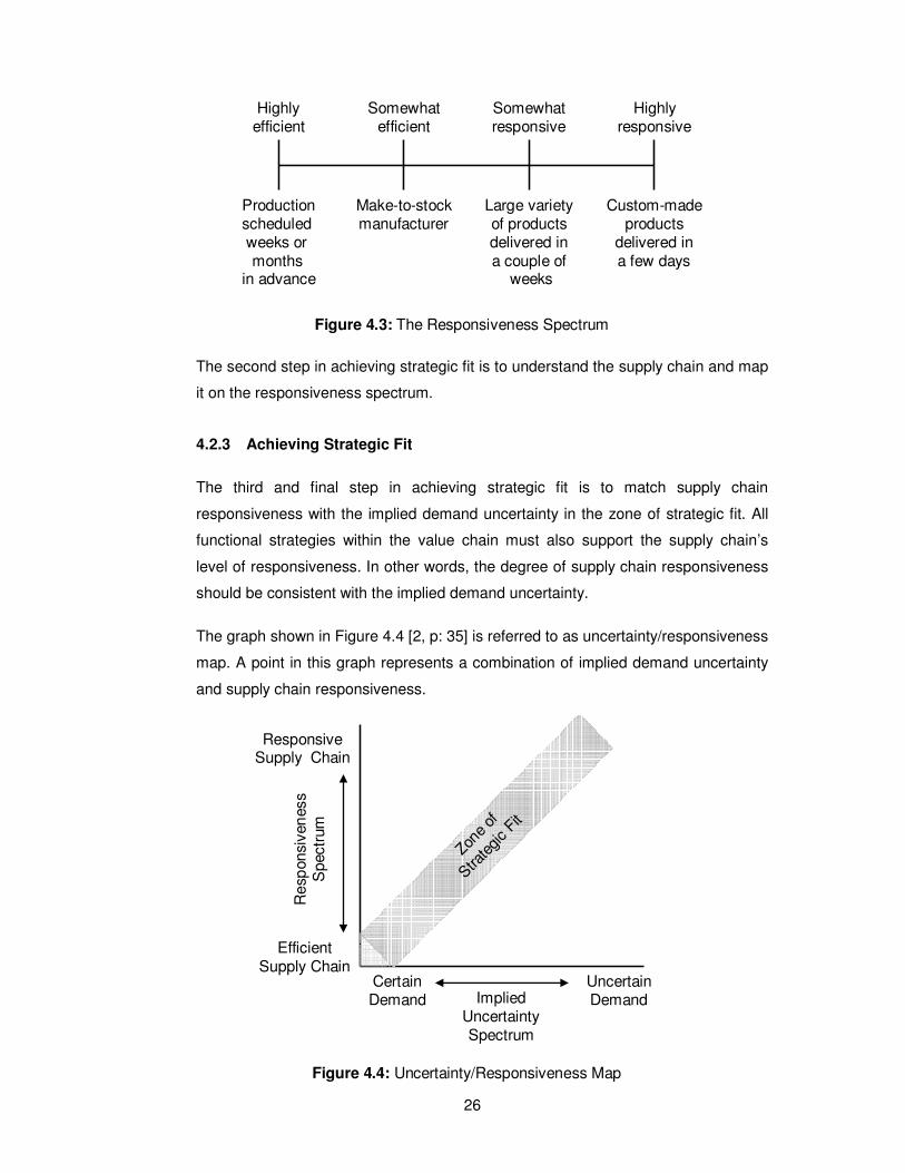
chain is the level of responsiveness it seeks to provide. Figure 4.3 [2, p: 33] shows

the responsiveness spectrum and where some different supply chains fall on this

spectrum.

Figure 4.2: Cost-Responsiveness Efficient Frontier

High

LowHigh

Low

Responsiveness

Cost

Figure 4.2: Cost-Responsiveness Efficient Frontier

High

LowHigh

Low

Responsiveness

Cost

High

LowHigh

Low

Responsiveness

Cost

26

The second step in achieving strategic fit is to understand the supply chain and map

it on the responsiveness spectrum.

4.2.3 Achieving Strategic Fit

The third and final step in achieving strategic fit is to match supply chain

responsiveness with the implied demand uncertainty in the zone of strategic fit. All

functional strategies within the value chain must also support the supply chain’s

level of responsiveness. In other words, the degree of supply chain responsiveness

should be consistent with the implied demand uncertainty.

The graph shown in Figure 4.4 [2, p: 35] is referred to as uncertainty/responsiveness

map. A point in this graph represents a combination of implied demand uncertainty

and supply chain responsiveness.

Figure 4.3: The Responsiveness Spectrum

Highlyefficient

Somewhatefficient

Somewhatresponsive

Highlyresponsive

Productionscheduled weeks or months

in advance

Make-to-stockmanufacturer

Large varietyof productsdelivered ina couple of

weeks

Custom-madeproducts

delivered ina few days

Figure 4.4: Uncertainty/Responsiveness Map

ResponsiveSupply Chain

ImpliedUncertaintySpectrum

CertainDemand

EfficientSupply Chain

UncertainDemand

Res

pon

sive

nes

sS

pect

rum

Zone

of

Strate

gic F

it

27

The implied demand uncertainty represents customer needs or the firm’s strategic

position. The supply chain’s responsiveness represents the supply chain strategy.

In order to achieve strategic fit, the greater the implied demand uncertainty, and the

more responsive the supply chain should be. Increasing implied demand uncertainty

from customers is best served with increasing responsiveness from the supply

chain. This relationship is represented by the zone of strategic fit. For a high level of

performance, companies should gear their competitive strategy toward the zone of

strategic fit.

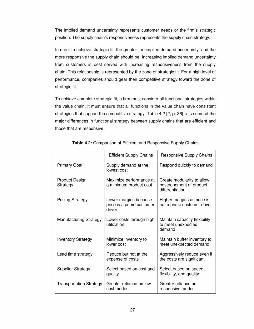
To achieve complete strategic fit, a firm must consider all functional strategies within

the value chain. It must ensure that all functions in the value chain have consistent

strategies that support the competitive strategy. Table 4.2 [2, p: 36] lists some of the

major differences in functional strategy between supply chains that are efficient and

those that are responsive.

Table 4.2: Comparison of Efficient and Responsive Supply Chains

Efficient Supply Chains Responsive Supply Chains

Primary Goal Product Design Strategy Pricing Strategy Manufacturing Strategy Inventory Strategy Lead time strategy Supplier Strategy Transportation Strategy

Supply demand at the lowest cost Maximize performance at a minimum product cost Lower margins because price is a prime customer driver Lower costs through high utilization Minimize inventory to lower cost Reduce but not at the expense of costs Select based on cost and quality Greater reliance on low cost modes

Respond quickly to demand Create modularity to allow postponement of product differentiation Higher margins as price is not a prime customer driver Maintain capacity flexibility to meet unexpected demand Maintain buffer inventory to meet unexpected demand Aggressively reduce even if the costs are significant Select based on speed, flexibility, and quality Greater reliance on responsive modes

28

4.2.3.1 Multiple Products and Customer Segments

Most companies produce and sell multiple products and serve multiple customer

segments, each with different characteristics. A department store may sell seasonal

products with high implied demand uncertainty along with products with low implied

demand uncertainty. The demand in each case maps to different parts of the

uncertainty spectrum. When devising supply chain strategy, the key issue for a

company is then to create a supply chain that balances efficiency and

responsiveness given its portfolio of products and customer segments.

There are several possible routes a company can take. One is to set up

independent supply chains for each different product or customer segment. This

strategy is feasible if each segment is large enough to support a dedicated supply

chain. A preferable strategy is to tailor the supply chain to best meet the needs of

each product’s demand, taking advantage of any economies of scope that often

exist between a company’s different products.

Tailoring the supply chain requires sharing some links in the supply chain with other

products while having separate operations for other links. The links are shared to

achieve maximum possible efficiency while providing the appropriate level of

responsiveness to each segment. Appropriate tailoring of the supply chain helps a

firm achieve varying levels of responsiveness for a low overall cost.

4.2.3.2 Product Life Cycle

As products go through their life cycles, the demand characteristics and the needs

of the customer segments being served change. High-tech products are particularly

prone to these life cycle swings over a very compressed time span. A product goes

through life cycle phases from the introductory phase, when only the leading edge of

customers is interested in it, all the way to the point at which the product becomes a

commodity and the market is completely saturated. To maintain strategic fit, a

company’s supply chain strategy must evolve as its products enter different phases.

As the product becomes a commodity product later in its life cycle demand becomes

more certain, margins are lower due to an increase in competitors, and price

becomes a significant factor in customer choice. As products mature, the

corresponding supply chain strategy should, in general, move from being responsive

to being efficient, as illustrated in Figure 4.5 [2, p: 39].

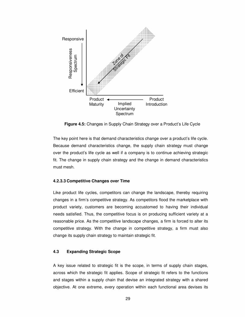
29

The key point here is that demand characteristics change over a product’s life cycle.

Because demand characteristics change, the supply chain strategy must change

over the product’s life cycle as well if a company is to continue achieving strategic

fit. The change in supply chain strategy and the change in demand characteristics

must mesh.

4.2.3.3 Competitive Changes over Time

Like product life cycles, competitors can change the landscape, thereby requiring

changes in a firm’s competitive strategy. As competitors flood the marketplace with

product variety, customers are becoming accustomed to having their individual

needs satisfied. Thus, the competitive focus is on producing sufficient variety at a

reasonable price. As the competitive landscape changes, a firm is forced to alter its

competitive strategy. With the change in competitive strategy, a firm must also

change its supply chain strategy to maintain strategic fit.

4.3 Expanding Strategic Scope

A key issue related to strategic fit is the scope, in terms of supply chain stages,

across which the strategic fit applies. Scope of strategic fit refers to the functions

and stages within a supply chain that devise an integrated strategy with a shared

objective. At one extreme, every operation within each functional area devises its

Figure 4.5: Changes in Supply Chain Strategy over a Product’s Life Cycle

Responsive

ImpliedUncertaintySpectrum

ProductMaturity

Efficient

ProductIntroduction

Res

pon

sive

nes

sS

pect

rum

Zone o

f

Strate

gic F

it

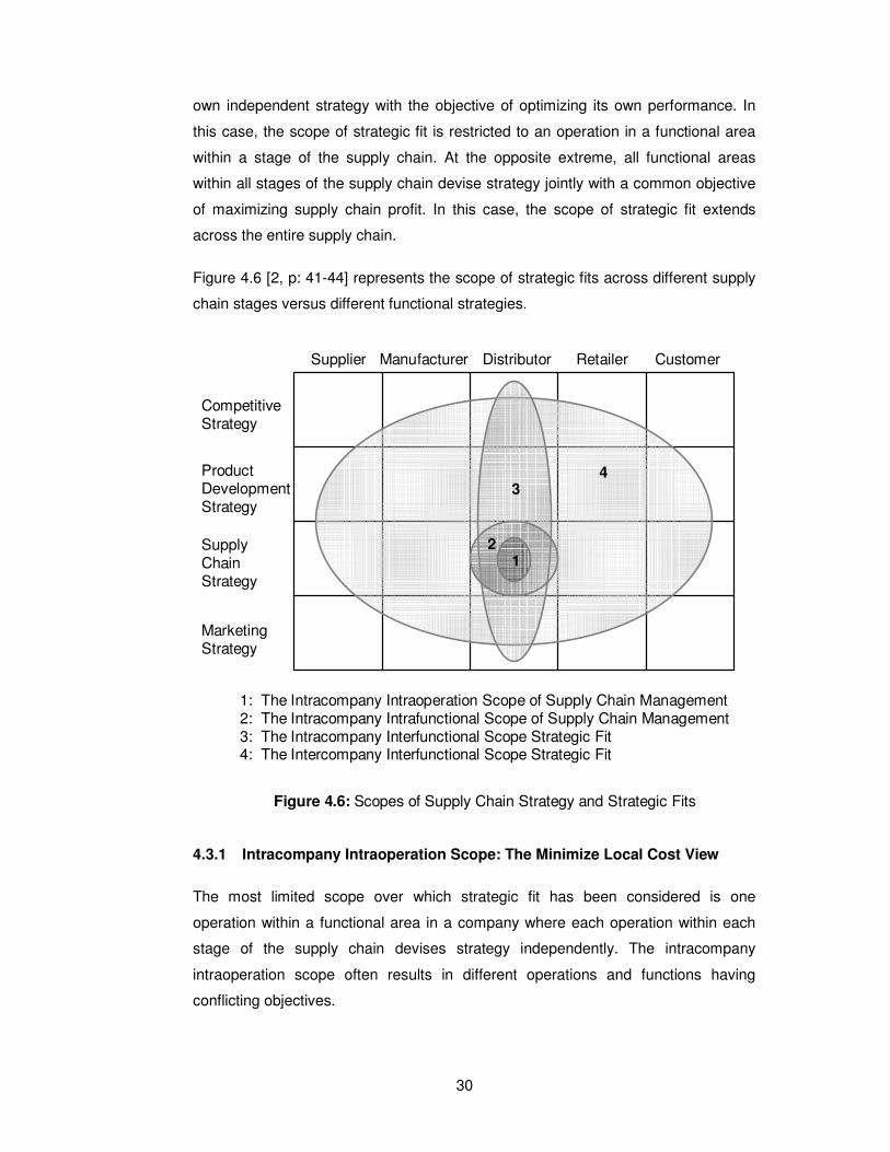
30

own independent strategy with the objective of optimizing its own performance. In

this case, the scope of strategic fit is restricted to an operation in a functional area

within a stage of the supply chain. At the opposite extreme, all functional areas

within all stages of the supply chain devise strategy jointly with a common objective

of maximizing supply chain profit. In this case, the scope of strategic fit extends

across the entire supply chain.

Figure 4.6 [2, p: 41-44] represents the scope of strategic fits across different supply

chain stages versus different functional strategies.

4.3.1 Intracompany Intraoperation Scope: The Minimize Local Cost View

The most limited scope over which strategic fit has been considered is one

operation within a functional area in a company where each operation within each

stage of the supply chain devises strategy independently. The intracompany

intraoperation scope often results in different operations and functions having

conflicting objectives.

Figure 4.6: Scopes of Supply Chain Strategy and Strategic Fits

Supplier Manufacturer Distributor Retailer Customer

CompetitiveStrategy

ProductDevelopmentStrategy

SupplyChainStrategy

MarketingStrategy

12

34

1: The Intracompany Intraoperation Scope of Supply Chain Management2: The Intracompany Intrafunctional Scope of Supply Chain Management3: The Intracompany Interfunctional Scope Strategic Fit4: The Intercompany Interfunctional Scope Strategic Fit

31

4.3.2 Intracompany Intrafunctional Scope: The Minimize Functional Cost

View

With the intracompany intrafunctional scope, the strategic fit is expanded to include

all operations within a function. The key weakness of the intracompany

intrafunctional view is that different functions may have conflicting objectives and

may hurt the firm’s overall performance.

4.3.3 Intracompany Interfunctional Scope: The Maximize Company Profit

View

With intracompany interfunctional scope, the goal is to maximize company profit. To

achieve this goal, all functional strategies are developed to support each other and

the competitive strategy. However, intracompany interfunctional scope of strategic fit

has still two major weaknesses.

The first derives from the fact that the only positive cash flow for the supply chain

occurs when the customer pays for the product. All other cash flows are simply a

resettling of accounts within the supply chain and add to supply chain cost. The

difference between what the customer pays and the total cost generated across the

supply chain represents the supply chain surplus. The supply chain surplus

represents the total profit to be shared across all companies in the supply chain.

Increasing supply chain surplus increases the amount to be shared among all

members of the supply chain. The intracompany interfunctional scope leads to each

stage of the supply chain trying to maximize its own profits, which does not

necessarily result in the maximization of the supply chain surplus. Supply chain

surplus is maximized only when all supply chain stages coordinate strategy

together.

The second major weakness of the intracompany scope becomes apparent when

speed becomes a key driver of supply chain success. The companies can succeed

not only because they have the lowest priced or highest quality products, but also

because they are able to respond quickly to market needs and get the right product

to the right customer at the right time. However, the most significant delays are

created at the interface between the boundaries of different stages of a supply

chain.

32

4.3.4 Intercompany Interfunctional Scope: The Maximize Supply Chain

Surplus View

The intercompany scope forces every stage of the supply chain to look across the

entire supply chain and evaluate the impact of its actions on other stages as well on

the interfaces. A company’s partners in the supply chain may well determine the

company’s success, as the company is intimately tied to its supply chain. This broad

scope increases the size of the surplus to be shared among all stages of the supply

chain. Intercompany view requires that each company evaluate its actions in the

context of the entire supply chain. Supply chain contracts help achieve this scope.

4.3.5 Flexible Intercompany Interfunctional Scope

Flexibility refers to a firm’s ability to achieve strategic fit when partnering with stages

that change over time in the supply chain. Firms must think in terms of supply chains

consisting of many partners at each stage. The flexible intercompany scope allows

strategic fit to apply to a moving target. Flexibility becomes more important as the

competitive environment becomes more dynamic.

4.4 Demand Driven Supply Chain

Supply chain surplus is maximized only when all supply chain stages coordinate

strategy together. However, a supply chain’s surplus is also significantly impacted

by demand. Revenues are typically higher when overall demand increases in

general. On the other hand, consumer demand for most products and services are a

function of the price the customer is willing to pay. If an increase in a product’s price

has a direct negative relationship with the total demand, this elasticity will create a

reduction or shift in the total demand. Therefore, price elasticity is a key factor

influencing the supply chain surplus and must be incorporated into supply chain

contracts and strategies aimed to achieve maximum surplus. In section 5, constant

and linear elasticity functions will be discussed and used as an integral part of any

supply chain contracts aimed to maximize the supply chain surplus.

Another key factor is to understand the demand patterns. The major demand

patterns are shown in Figure 4.7 [74, p: 30]. A constant/horizontal pattern with

normally distributed demand where the mean demand is a function of the selling

price is used in this dissertation.

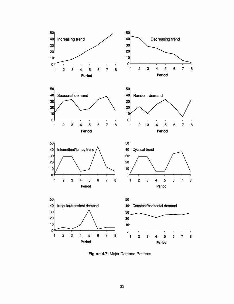
33

Figure 4.7: Major Demand Patterns

0

10

20

30

40

50

1 2 3 4 5 6 7 8

Period

Increasing trend

0

10

20

30

40

50

1 2 3 4 5 6 7 8

Period

Decreasing trend

0

10

20

30

40

50

1 2 3 4 5 6 7 8

Period

Seasonal demand

0

10

20

30

40

50

1 2 3 4 5 6 7 8

Period

Random demand

0

10

20

30

40

50

1 2 3 4 5 6 7 8

Period

Increasing trend

0

10

20

30

40

50

1 2 3 4 5 6 7 8

Period

0

10

20

30

40

50

1 2 3 4 5 6 7 8

Period

Decreasing trend

0

10

20

30

40

50

1 2 3 4 5 6 7 8

Period

0

10

20

30

40

50

1 2 3 4 5 6 7 8

Period

Seasonal demand

0

10

20

30

40

50

1 2 3 4 5 6 7 8

Period

0

10

20

30

40

50

1 2 3 4 5 6 7 8

Period

Random demand

Intermittent/lumpy trend Cyclical trend

Irregular/transient demand Constant/horizontal demand

0

10

20

30

40

50

1 2 3 4 5 6 7 8

Period

0

10

20

30

40

50

1 2 3 4 5 6 7 8

Period

0

10

20

30

40

50

1 2 3 4 5 6 7 8

Period

0

10

20

30

40

50

1 2 3 4 5 6 7 8

Period

Intermittent/lumpy trend Cyclical trend

Irregular/transient demand Constant/horizontal demand

0

10

20

30

40

50

1 2 3 4 5 6 7 8

Period

0

10

20

30

40

50

1 2 3 4 5 6 7 8

Period

0

10

20

30

40

50

1 2 3 4 5 6 7 8

Period

0

10

20

30

40

50

1 2 3 4 5 6 7 8

Period

0

10

20

30

40

50

1 2 3 4 5 6 7 8

Period

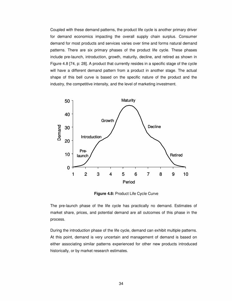
34

Coupled with these demand patterns, the product life cycle is another primary driver

for demand economics impacting the overall supply chain surplus. Consumer

demand for most products and services varies over time and forms natural demand

patterns. There are six primary phases of the product life cycle. These phases

include pre-launch, introduction, growth, maturity, decline, and retired as shown in

Figure 4.8 [74, p: 28]. A product that currently resides in a specific stage of the cycle

will have a different demand pattern from a product in another stage. The actual

shape of this bell curve is based on the specific nature of the product and the

industry, the competitive intensity, and the level of marketing investment.

The pre-launch phase of the life cycle has practically no demand. Estimates of

market share, prices, and potential demand are all outcomes of this phase in the

process.

During the introduction phase of the life cycle, demand can exhibit multiple patterns.

At this point, demand is very uncertain and management of demand is based on

either associating similar patterns experienced for other new products introduced

historically, or by market research estimates.

Figure 4.8: Product Life Cycle Curve

Introduction

Pre-launch

Growth

Maturity

Decline

Retired

0

10

20

30

40

50

1 2 3 4 5 6 7 8 9 10

Period

Dem

and

Introduction

Pre-launch

Growth

Maturity

Decline

Retired

0

10

20

30

40

50

1 2 3 4 5 6 7 8 9 10

Period

Dem

and

35

As products reach the growth phase, demand becomes more stable and

predictable. Demand management can use trends and statistics to define the

pattern accurately.

During the maturity phase, demand is quite stable. As products mature, the

corresponding supply chain strategy should, in general, move from being responsive

to being efficient, as previously illustrated in Figure 4.5. The demand functions used

in this dissertation assume that the products are in their maturity phases.

Predicting demand during the decline phases is often the most difficult. The intensity

and timing of the decline make it very difficult to understand the demand pattern.

The best way to analyze the product’s decline is to explore historical similar product

declines and associate a similar intensity and timing evidenced in other products

and categories. Prices tend to be at historical lows during the decline phase.

At the retired phase, the product has been phased out. All demand that existed has

either been transferred to a complementary or replacement item, or has been

moved to a competitor’s product.

In summary, each of the phases of the life cycle result in changes to the demand

pattern, and likewise require a different type of technique to analyze and manage

demand. The use of collaboration within the chain is essential during all phases of

the product life cycle in order to achieve improved and accurate forecasts.

4.5 Supply Chain Performance Drivers

The strategic fit requires that a company achieve the balance between

responsiveness and efficiency in its supply chain that best meets the needs of the

company’s competitive strategy [75-80]. The drivers of supply chain performance

not only determine its performance in terms of responsiveness and efficiency, they

also determine whether strategic fit is achieved across the supply chain [2, p: 49-

60]. The five drivers of supply chain performance are:

• Inventory

• Transportation

• Facilities

• Information

• Contracts

36

Inventory is all raw materials, work in process, and finished goods within a supply

chain. Inventory is an important supply chain driver because changing inventory

policies can dramatically alter the supply chain’s efficiency and responsiveness.

Transportation entails moving inventory from point to point in the supply chain.

Transportation can take the form of many combinations of modes and routes, each

with its own performance characteristics and transportation choices have a large

impact on supply chain responsiveness and efficiency.

Facilities are the places in the supply chain network where inventory is stored,

assembled, or fabricated. The two major types of facilities are production sites and

storage sites. Whatever the function of the facility, decisions regarding location,

capacity, and flexibility of facilities have a significant impact on the supply chain’s

performance.

Information consists of data and analysis regarding inventory, transportation, and

customers throughout the supply chain. Information is potentially the biggest driver

of performance in the supply chain as it directly affects the other drivers.

Contracts are most effective for governance and specify the parameters within

which a buyer places orders and a supplier fulfills them. Contracts can potentially

increase the total supply chain surplus and they are the core subject of this

dissertation. Contracts will be discussed in details in Chapter 6.

4.5.1 Inventory

Increasing the inventory will generally make the supply chain more responsive to the

customer. However, this choice comes as at a cost as the added inventory

decreases efficiency [81-86].

4.5.1.1 Role in the Supply Chain

Inventory exists in the supply chain because of a mismatch between supply and

demand. This mismatch is intentional at the retailer in anticipation of future demand.

An important role that inventory plays in the supply chain is to increase the amount

of demand that can be satisfied by having the product ready and available when the

customer wants it. Supply Chain contracts play a significant role to achieve this

purpose. Another significant role inventory plays is to reduce cost by exploiting any

economies of scale that may exist during both production and distribution.

37

Inventory is spread throughout the supply chain from raw materials to work in

process to finished goods that suppliers, manufacturers, distributors, and retailers

hold. Inventory is a major source of cost in a supply chain, and it has a huge impact

on responsiveness.

Inventory has also a significant impact on the material flow time in a supply chain

defined as the time that elapses between the point at which material enters the

supply chain to the point at which it exits. Another important area where inventory

has a significant impact is throughput, the rate at which sales to the end customer

occur. If inventory is represented by I, flow time by T, and throughput by R, the three

can be related as [2, p: 52]:

I = RT (4.1)

Reduced flow time can be a significant advantage in a supply chain by reducing the

inventory needed without reducing responsiveness.

4.5.1.2 Role in the Competitive Strategy

Inventory plays a significant role in a supply chain’s ability to support a firm’s

competitive strategy. If a firm’s competitive strategy requires a very high level of

responsiveness, a company can use inventory to achieve this responsiveness by

allocating large amounts of inventory close to the customer. Conversely, a company

can also use inventory to make itself more efficient by reducing inventory through

centralized stocking. The latter strategy would support a competitive strategy of

being a low cost producer. The trade-off implicit in the inventory driver is between

the responsiveness that results from more inventory and the efficiency that results

from less inventory.

4.5.1.3 Components of Inventory Decisions

Major inventory related decisions to create more responsive and more efficient

supply chains involve cycle inventory, safety inventory, and seasonal inventory.

Cycle inventory is the average amount of inventory used to satisfy demand between

receipts of supplier shipments. The size of the cycle inventory is a result of the

production or purchase of materials in large lots to exploit economies of scale in the

production, transportation, or purchasing process. The basic trade-off is the cost of

holding larger lots of inventory versus the cost of ordering the product frequently.

38

Safety inventory is held just in case demand exceeds expectations to counter

uncertainty. Choosing safety inventory involves making a trade-off between the

costs of having too much inventory and the costs of lost sales due to not having

enough inventory.

Seasonal inventory is built up to counter predictable variability in demand.

Companies using seasonal inventory will build up inventory in periods of low

demand and store it for periods of high demand when they will not have the capacity

to produce all that is demanded. If a company can rapidly change the rate of its

production system at low cost, then it may not need seasonal inventory. The basic

trade-off is the cost of carrying the additional seasonal inventory versus the cost of

having a more flexible production rate.

4.5.2 Transportation

The fundamental trade-off for transportation is between efficiency, the cost of

transporting a given product, and responsiveness, the speed with which the product

is transported [87-93].

4.5.2.1 Role in the Supply Chain

Transportation moves the product between different stages in a supply chain. Like

the other supply chain drivers, transportation has a large impact on both

responsiveness and efficiency. Faster transportation, whether in the form of different

modes of transportation or different amounts being transported, allows a supply

chain to be more responsive but reduces its efficiency. The type of transportation a

company uses also affects the inventory and facility locations in the supply chain.

4.5.2.2 Role in the Competitive Strategy

The role of transportation in a company’s competitive strategy figures prominently

when the company is considering the target customer’s need. If its competitive

strategy targets a customer that demands a very high level of responsiveness and

that customer is willing to pay for this responsiveness, then a company can use

transportation as one driver for making the supply chain more responsive. On the

other hand, if it targets customers whose main criterion is price, then the company

can use transportation to lower the cost of the product at the expense of

responsiveness.

39

As a company may use both inventory and transportation to increase

responsiveness or efficiency, the optimal decision for the company often means

finding the right balance between the two.

4.5.2.3 Components of Transportation Decisions

Major transportation related decisions to create more responsive and more efficient

supply chains involve mode of transportation, route and network selection, and in

house or outsource decisions.

The mode of transportation is the manner in which a product is moved from one

location in the supply chain network to another. Companies have four basic modes

from which to choose. In decreasing responsiveness, companies may choose air,

truck, rail, or ship transportation modes. Depending on the product, pipeline and

electronic transportation can also be used. Each mode has different characteristics

with respect to the speed, size of shipments, cost of shipping, and flexibility that lead

companies to choose one particular mode over the others.

Another major transportation decision is the route and network along which products

are shipped. A route is the path along which a product is shipped, and a network is

the collection of locations and routes along which a product can be shipped. A

company may need to decide whether to ship products directly to customers or to

use a series of distribution layers. Companies make some routing decisions at the

supply chain’s design stage, and they make others on a short term basis.

Traditionally, much of the transportation function has been performed in house.

Today, however, much of transportation, even entire logistics systems, is

outsourced. Having to choose between bringing parts of transportation in house or

outsourcing leads to another dimension of complexity when companies are

designing their transportation systems. In this dissertation, transportation related

costs are not considered separately, but rather assumed to be included in the unit

price.

4.5.3 Facilities

The fundamental trade-off for facilities is between efficiency, the cost of the number,

location, and type of facilities, and the level of responsiveness that these facilities

provide the company’s customers [88, 94-98].

40

4.5.3.1 Role in the Supply Chain

If inventory is what is being passed along the supply chain and transportation as

how it is passed along, then facilities are the where of the supply chain. They are the

locations to or from which the inventory is transported. Within a facility, inventory is

either transformed into another state, manufacturing, or stored before being shipped

to the next stage, warehousing.

4.5.3.2 Role in the Competitive Strategy

Facilities and their corresponding capacities to perform their functions is a key driver

of supply chain performance in terms of responsiveness and efficiency. Companies

may gain economies of scale when a product is manufactured or stored in only one

location. This centralization increases efficiency. However, the cost reduction comes

at the expense of responsiveness, as many of company’s customers may be located

far from the production facility. On the other hand, locating facilities close to

customers increases the number of facilities needed and consequently reduces

efficiency. However, if the customer demands and is willing to pay for the

responsiveness that having numerous facilities adds, then this facilities decision

helps meet the company’s competitive strategy goals.

4.5.3.3 Components of Facilities Decisions

The components of facilities decisions are the location, capacity, manufacturing

methodology, and various warehousing methodologies.

Deciding where a company will locate its facilities constitutes a large part of the

design of a supply chain. A basic trade-off is whether to centralize to gain

economies of scale or decentralize to become more responsive by being closer to

the customer. Companies must also consider related issues to the characteristics of

the local area in which the facility may be situated. These include macroeconomic

factors, strategic factors, quality and cost of workers, cost of facility, availability of

infrastructure, proximity to customers and the rest of the network, and tax effects.

Companies must also decide what a facility’s capacity to perform its intended

function or functions will be. A large amount of excess capacity allows the facility to

be very flexible and to respond to wide swings in the demands placed on it. Excess

capacity, however, costs money and therefore can decrease efficiency. A facility

with little excess capacity will likely be more efficient per unit of product it produces

41

than one with a lot of unused capacity. On the other hand, the high utilization facility

will have difficulty responding to demand fluctuations. Therefore a company must

make a trade-off between flexibility and efficiency to determine the right amount of

capacity to have at each of its facilities.

Companies must also make a major decision regarding the manufacturing

methodology that a facility will use. They must decide whether to design a facility

with a product focus or a functional focus. A product focused factory performs many

different functions, such as fabrication and assembly, in producing a single type of

product. A functional focused factory performs few functions, such as only

fabrication or only assembly, on many types of products. A product focus tends to

result in more expertise about a particular type of product at the expense of the

functional expertise that comes from a functional manufacturing methodology.

Companies must decide which type of expertise will best enable them to meet

customer needs. They must also make a decision regarding the relative level of

flexible versus dedicated capacity in their portfolios. Flexible capacity can be used

for many types of products but is often less efficient whereas the more efficient

dedicated capacity can be used for only a limited number of products. The trade-off

is again between efficiency and responsiveness.

As with manufacturing, there are a variety of methodologies from which companies

can choose when designing a warehouse facility, including Stock-keeping Unit

(SKU) storage, Job Lot Storage, and Crossdocking.

4.5.4 Information

Many information systems increase both responsiveness and efficiency. The trade-

off is between the cost of information which comes with a reduction in efficiency and

the responsiveness that information creates in the supply chain.

4.5.4.1 Role in the Supply Chain

Information could be overlooked as a major supply chain driver because it does not

have a physical presence. Information, however, affects every part of the supply

chain in many ways [99-108]. It serves as the connection between the supply

chain’s various stages, allowing them to coordinate their actions and bring about

many of the benefits of maximizing total supply chain profitability. Information is also

crucial to the daily operations of each stage in a supply chain.

42

4.5.4.2 Role in the Competitive Strategy

Information is a driver whose importance has grown as companies have used it to

become both more efficient and responsive. The tremendous growth of the

importance of information technology is a testimony to the impact information can

have on improving a company. However, like the other drivers, even with

information, companies reach a point where they must make the trade-off between

efficiency and responsiveness.

Another key decision involves what information is most valuable in reducing cost

and improving responsiveness within a supply chain. This decision will vary

depending on the supply chain structure and the market segments served.

4.5.4.3 Components of Information Decisions

Key components of information within a supply chain to increase efficiency and

improve responsiveness are push versus pull, coordination and information sharing,

forecasting and aggregate planning, and enabling technologies.

When designing processes in the supply chain, managers must determine whether

these processes are part of the push or pull phase in the chain. Push systems

generally require information in the form of elaborate material requirements planning

(MRP) systems to take the master production schedule and roll it back, creating

schedules for suppliers with part types, quantities, and delivery dates. Pull systems

require information on actual demand to be transmitted extremely quickly throughout

the entire chain so that production and distribution of parts and products can

accurately reflect the real demand. Just-in-time (JIT) production is often referred as

a pull system.

Supply chain coordination occurs when all the different stages of a supply chain

work toward the objective of maximizing total supply chain profitability, rather than

each stage devoting itself to its own profitability. Again, supply chain contracts can

play a significant role to achieve this objective. Lack of coordination may result in a

significant loss of total supply chain profit. Coordination between different stages in

a supply chain requires each stage to share appropriate information with other

stages.

43

Forecasting is the art and science of making projections about what future needs

and conditions will be. Obtaining forecasting information frequently means using

sophisticated techniques to estimate future demand or market conditions.

Companies often use forecasts both on a tactical level to schedule production and

on a strategic level to determine whether to build new plants or even whether to

enter a new market. Aggregate planning transforms forecasts into plans of activity to

satisfy the projected demand. A company’s aggregate plan significantly affects the

demand on both its suppliers and its supply to its customers.

Today, many technologies exist that share and analyze information in the supply

chain [109-112]. The technologies include Electronic Data Interchange (EDI), the

Internet, Enterprise Resource Planning (ERP), Supply Chain Management (SCM)

software, and Advanced Planning and Scheduling (APS). As we will see in Chapter

5, these technologies are vital for successful supply chain contract implementations.

4.6 Obstacles to Achieving Strategic Fit

A company’s ability to find a balance between responsiveness and efficiency along

the responsiveness spectrum that best matches the type of demand it is targeting is

the key to achieving strategic fit. In deciding where this balance should be located

on the responsiveness spectrum, companies must overcome the following

obstacles. Many of these obstacles have made it increasingly difficult for supply

chains to achieve strategic fit [2, p: 60-62]. Overcoming these obstacles offers a

tremendous opportunity for firms to use supply chain performance drivers, including

supply chain contracts, to gain competitive advantage.

4.6.1 Increasing Variety of Products

With customers demanding ever more customized products, manufacturers have

responded with mass customization. The increase in product variety complicated the

supply chain by making forecasting and meeting demand much more difficult. The

rise of e-commerce, which makes it easy to offer variety to the customer, reinforces

the customization trend. Increase variety tends to raise uncertainty, and uncertainty

frequently results in increased cost and decreased responsiveness within the supply

chain. Again, supply chain contracts can help overcome this obstacle.

44

4.6.2 Decreasing Product Life Cycles

In addition to the increasing variety of product types, the life cycle of products has

been shrinking. This decrease in product life cycles makes the job of achieving

strategic fit more difficult, as the supply chain must constantly adapt to manufacture

and deliver new products in addition to coping with these product’s demand

uncertainty. Shorter life cycles increase uncertainty while reducing the window of

opportunity within which the supply chain can achieve strategic fit. Increased

uncertainty combined with a smaller window of opportunity has put additional

pressure on supply chains to coordinate and create a good match between supply

and demand. Once again, supply chain contracts can be used to create this match.

4.6.3 Increasingly Demanding Customers

Companies can clearly see how customer demands have increased when

considering delivery lead times, cost, and product performance. Today’s customers

are demanding faster fulfillment, better quality, and better performing products for

the same price they paid years ago meaning that the supply chain must provide

more just to maintain its business.

4.6.4 Fragmentation of Supply Chain Ownership

Over the past several decades, most firms have become less vertically integrated.

As companies have shed noncore functions, they have been able to take advantage

of supplier and customer competencies that they themselves did not have. However,

this new ownership structure has also made managing the supply chain more

difficult. With the chain broken into many owners, each with its own policies and

interests, the chain is more difficult to coordinate. Potentially, this problem could

cause each stage of a supply chain to work only toward its own objectives rather

than the whole chain’s, resulting in the reduction of overall supply chain profitability.

As we will see in Chapter 6, supply chain contracts can be used very effectively to

overcome this obstacle.

4.6.5 Globalization

The increase in globalization over the past few decades has had two main impacts

on the supply chain. The first impact is that supply chains are now more likely than

ever to be global. Having a global supply chain creates many benefits, such as the

45

ability to source from a global base of suppliers who may offer better and cheaper

goods than were available in a company’s home nation. However, globalization also

adds stress to the chain because facilities within the chain are farther apart, making

coordination more difficult.

The second impact of globalization is an increase in competition. This competitive

situation makes supply chain performance a key to maintaining and growing sales

while also putting more strain on supply chains and thus forcing them to make their

trade-offs even more precisely.

4.6.6 Difficulty in Executing New Strategies

Creating a successful supply chain strategy is not easy. However, once a good

strategy is formulated, actually executing the strategy can even be more difficult.

Many high talented employees at all levels of the organization are necessary to

make a supply chain strategy successful. The increasing impact of all these

obstacles has led to supply chain management becoming a major factor in the

success or failure of firms.

4.7 Managing Predictable Variability

As discussed in Section 4.5, aggregate planning transforms forecasts into plans of

activity to satisfy the projected demand. A company’s aggregate plan significantly

affects the demand on both its suppliers and its supply to its customers. For

products whose demand is stable with little change in volume over time, devising an

aggregate plan is simple. In such cases, a company arranges for sufficient capacity

to match the expected demand and then produces an amount to match that

demand. Products are made close to the time when they will be sold. The supply

chain carries little inventory [2, p: 121-127].

However, demand for many products changes from period to period, often due to a

predictable influence such as seasonal factors and promotions [113-116].

Predictable demand is the change in demand that can be forecasted. Products that

undergo this type of change in demand cause numerous problems in the supply

chain, ranging from high levels of stockouts during peak demand periods to high

levels of excess inventory during periods of low demand. These problems increase

the cost of products and decrease the responsiveness of the supply chain. Supply

46

and demand management will have the greatest impact when it is applied to

predictably variable products.

A company must choose between two broad options to handle predictable

variability: managing supply and managing demand.

4.7.1 Managing Supply

Supply of products can be controlled by a combination of production capacity and

inventory. When managing capacity to meet predictable demand, companies use a

combination of the following approaches:

• Time flexibility from workforce

• Use of seasonal workforce

• Use of subcontracting

• Use of both dedicated and flexible facilities

• Designing product flexibility into the production processes

When managing inventory to meet predictable variability, companies use a

combination of the following approaches:

• Using common components across multiple products

• Build inventory of high demand or predictable demand products

4.7.2 Managing Demand

In many instances, supply chains can influence demand in different periods using

pricing and other forms of promotion. When a promotion is offered during a period,

that period’s demand will tend to go up. This increase in demand results from a

combination of the following factors:

• Market growth

• Stealing share

• Forward buying

The first two factors increase the overall demand whereas the third simply shifts

future demand to the present.

In Chapter 6, we will discuss how product availability and supply chain profits are

affected by contracts between stages of the supply chain. Effective use of contracts

47

as a supply chain driver can substantially increase the overall supply chain

profitability and its competitive advantage.

4.8 Implications of Supply Chain Management in Agile Manufacturing

Supply chain management evolution has provided a number of practices that

directly relate to improving agility within and between organizations [117-128].

Changing customer and technological requirements force manufacturers to develop

agile supply chain capabilities in order to be competitive. The requirements for

organizations to become more responsive to the needs of customers, the changing

conditions of competition, and increasing levels of environmental turbulence is

driving the concept of agility. The concept has also been extended beyond the

traditional boundaries of the individual organization to encompass the operations of

the supply chain within which the organization operates. It is imperative for

companies to cooperate and leverage complementary competencies such as using

market knowledge and a virtual corporation to exploit profitable opportunities in a

volatile marketplace. There has also been much research combining the lean

philosophy and agile manufacturing [129-135].

Agility performance factors such as time, cost, flexibility, dependability are all

affected by the management of the supply chain. The following have been defined

as exemplary practices for strategic supplier relationships [136, p: 361]:

• Development of long term, performance oriented supplier partnerships,

• Continuous quality improvement and joint learning by both the customer and its supplier base,

• Focus on total cost of ownership, not just on price,

• Companies are taking a boundaryless view of their participation in the supply chain,

• Long term contracts,

• Multi level relationship across the organization including inter company project teams,

• Critical buying decision based on value,

• Early involvement in marketing, design, and product development cycle,

• Exchange of information including not only information on work in progress, but also information on basic costs and insight into long term strategy,

• Integrated quality control,

• Mutual support and joint problem solving,

• Joint teams sharing information and expertise,

48

• A genuine insight into the buy decision and market forces up and down the supply chain, and

• Two or three suppliers at most, with single sourcing agreements, thus enabling the purchasing, engineering, production, and quality personnel to work more closely.

Strategic supplier relationships exist in a number of industries and are on the rise.

Supply chain contracts are part of these partnerships and alliances.

49

CHAPTER 5. INFORMATION TECHNOLOGY STRUCTURE AND SUPPLY

CHAIN CONTRACTS

The impact of technology upon the development and rapid expansion of supply

chain collaboration has been profound. In this chapter, we will discuss how

technology drives and facilitates supply chain integration, a vital necessity for

successful supply chain contract implementations.

5.1 Information Networks

Supply chain information systems initiate activities and track information regarding

processes and facilitates information sharing both within the firm and between

supply chain partners resulting to successful supply chain contracts. All component

systems must be integrated to provide comprehensive functionality for analyzing,

initiating, and monitoring supply chain operations [137, p: 191-196], thus facilitating

the supply chain contracts with timely and accurate information.

5.1.1 Information System Functionality

There are four reasons why timely and accurate information is vital. First, customers

perceive information about order status, product availability, delivery schedule,

shipment tracking, and invoices as necessary elements of total customer service.

Customers demand access to real time information. Second, with the goal of

reducing total supply chain assets, thus supply chain profitability, information can be

used to reduce inventory and human resource requirements, especially by

minimizing demand uncertainty. Third, information increases flexibility in supply

chain contracts with regard to how, when, and where resources may be utilized to

gain strategic advantage. Fourth, enhanced information transfer and exchange

capability utilizing the Internet is changing relationships between buyers and sellers

and redefining channel relationships. Supply chain information systems (SCIS)

provide integration on four levels of functionality: transaction systems, management

control, decision analysis, and strategic planning.

50

A transaction system is characterized by formalized rules, procedures, and

standardized communications [138-141]. The combination of structured processes

and large transaction volume initiated by supply chain contracts places a major

emphasis on information system efficiency on transaction activities including, but not

limited to, order entry, inventory assignment, order selection, shipment, pricing,

invoicing, and customer inquiry. The customer order performance cycle is completed

through a series of information system transactions.

The second level, management control, focuses on performance measurement and

reporting. Performance measurement is necessary to provide feedback for supply

chain contracts regarding performance and resource utilization. While some control

measures, such as cost, are well defined, other measures, such as customer

service and quality, are less specific. While internal measures are relatively easy to

track, external measures are more difficult to obtain since they require monitoring

performance regarding specific customers.

The third level, decision analysis, focuses on software tools to assist supply chain

partners in identifying, evaluating, and comparing strategic and tactical alternatives

for improved contract effectiveness. Decision analysis should also include a

centralized database and reporting over a wide range of potential logistics

situations. Decision analysis applications are also being used to manage customer

relationships by determining the trade-offs associated with having satisfied

customers. Because decision analysis is used to guide future contracts, thus

operations, users require more expertise and training to benefit from its capability.

Finally, as we will develop in Chapter 6, strategic planning can be used to organize

and synthesize transaction data into a wide range of business planning and decision

making models that assist in evaluating the probabilities and payoffs of various

strategies with the main focus on enhanced supply chain system integration.

5.1.2 Communication Systems

Information technology is also critical for information sharing to facilitate logistics

and supply chain planning and operations. Historically, coordination of logistics has

been difficult since logistics activities are often performed at locations distant from

information technology hardware. As a result, information was not available at the

location of essential work in terms of both time and content. The past decade has

witnessed remarkable advances in logistical communication systems capability. EDI,

51

the Internet, Extensible Markup Language (XML), and satellite technology exist to

facilitate communication between firms and facilities. Radio frequency allows short-

range communication within facilities such as warehouses. Image, bar coding, and

scanner technologies allow communication between supply chain information

systems and their physical environment.

While further communication system improvement will continue to reduce

uncertainty, it is likely that major opportunities for future performance enhancers will

be through supply chain analysis and strategic planning systems, including supply

chain contracts.

5.2 Enterprise Resource Planning (ERP) and Execution Systems

Enterprise Resource Planning (ERP) and execution systems are the major software

components of logistical information systems [142-144]. ERP provides the central

database and the transaction capability to initiate, track, monitor, and report on

customer and replenishment orders to further refine supply chain contracts. ERP

systems provide firms with information consistency, economies of scale, and

integration.

ERP system design includes the central database and application modules to

facilitate supply chain, financial, and human resource management. Supply chain

system design includes components for planning and coordination of operations and

inventory deployment.

Enterprise execution systems provide the interface between the ERP and the day-

to-day operations with the customer, transportation, and the warehouse. On the

other hand, Customer Relationship Management (CRM) systems offer ‘insight

regarding the firm’s activity level and performance with key customers. Benefits of

within the context of supply chain contracts can be summarized as:

• Quickened information response time,

• Increased interaction across the supply chain,

• Improved order management and order cycle,

• Decreased financial close cycle,

• Improved interaction with customers,

• Improved on-time delivery,

• Improved interaction with suppliers,

52

• Reduced direct operating costs, and

• Lowered inventory levels.

Gaining strategic advantage, the outcome of a successful supply chain contract, is

listed as one of the top motivations to implement ERP systems [145, p: 5-7]

5.2.1 Rationale for ERP Implementation

Regardless the size of the firms in the supply chain, ERP investments are typically

rationalized through three factors: consistency, economies of scale, and integration

[130, p: 223].

The first major ERP objective is to create a system that utilizes consistent data and

processes. In a typical application, the data is resident in a common data warehouse

that can be accessed globally. In addition, the data can be modified with appropriate

security and controls using transactions available in the supply chain. Transactions

are initiated by specific supply chain activities and implemented using common

assumptions and timing. Such a unified perspective offers supply chain partners a

consistent integrated view.

As firms merged and expanded, management made increasing demands to take

advantage of global scale economies through resource utilization. ERP offers firms

potential economies of scale in several ways. First, a single centralized processor or

a network of decentralized processors with common configurations offers the

potential for substantial procurement and maintenance scale economies. Second,

the centralized ERP approach offers significant software scale economies since only

a limited number of software licenses are necessary within the supply chain. Third,

potential scale economies for ERP expertise exists since relatively few individuals

have developed extensive skills. Finally, the centralized ERP approach increases

the potential for shared resources and services. All those economies of scale can

and should be factored into supply chain contracts.

Integration results from a common integrated database and implementation of

common processes. Typical common processes in ERP include order entry, order

processing, warehouse management, invoicing, and accounting. Such integration

also results in standard financial practices within the supply chain. A new generation

of ERP systems, identified as ERP II, integrate traditional ERP along with a

Customer Relationship Management (CRM) system to better integrate the

53

requirements and expectations of key customers. ERPII is the external connectivity

critical for supply chain collaboration.

5.2.2 Enterprise Execution Systems

ERP systems are substantially enhancing process and information consistency and

integration of supply chain operations. Yet the focus on integrated processes has

generally reduced the system functionality and features, particularly for operational

elements such as warehouse and transportation management. The result is that

ERP modules may not be capable of performing some of the major activities,

particularly those focused on enhancing value required to support supply chain

operations. Enterprise execution systems, including CRM, TMS, and WMS are

evolving to meet these specific requirements as they are very important factors in

successful supply chain contract implementations.

5.2.2.1 Customer Relationship Management (CRM)

CRM is designed to extend the functionality of the ERP sales and delivery

applications. Firms are using CRM to transition from treating customers as income

sources to be exploited to treating as assets to be nurtured [137, p: 241]. While the

traditional sales and delivery application was designed to accept customer orders in

a wide range of formats and allow those orders to be managed throughout the

fulfillment process, a broader range of capabilities is necessary to manage the

customer relationship. Beyond this basic functionality, CRM requires sales tracking,

sales history analysis, pricing management, promotion management, product mix

management, and category management, all providing vital information for supply

chain profitability and, implicitly, for supply chain contracts. For example, it is

becoming more common for grocers to expect their suppliers to manage both the

product mix and the shelf quantities for major product categories. This practice

which can be factored in supply chain contracts requires substantial information

support from the manufacturer but also facilitates information sharing.

5.2.2.2 Transportation Management System (TMS)

In general, the advanced TMS should proactively identify and evaluate alternative

transportation strategies and tactics to determine the best methods to move product

within the existing constraints. The principal deliverables of TMS are cost savings

54

and increased functionalities. Coupled with a supply chain contract, TMS can

provide:

• Order consolidation,

• Route optimization,

• Carrier rate management,

• EDI links with carriers,

• Internet-based shipment tracking, and

• Integrated claims management.

5.2.2.3 Warehouse Management System (WMS)

Historical warehouse system functionality focused on receiving replenishment

shipments, stock putaway, and order picking. Warehouses today must offer a

broader range of services as they are frequently performing some light

manufacturing. They also require managing more inventory on a just-in-time basis.

Advanced WMS functionalities include:

• Yard management, which refers to the process of managing the vehicles

and the inventory within vehicles while in the warehouse yard,

• Labor management to maximize the use of warehouse labor,

• Warehouse optimization to select the best location within the warehouse

for the storage and retrieval of products to minimize time and movement,

• Value Added Services (VAS) to coordinate various warehouse activities

to customize products, such as labelling, kitting, and setting up displays,

• Planned cross-docking and merging, which refers to the integration of

two parts of a customer order that have been supplied from a different

source without maintaining inventory, and

• Reverse logistics activities such as returns, repair, and recycling.

5.3 Advanced Planning and Scheduling (APS)

Advanced Planning and Scheduling (APS) systems work with ERP systems by

providing business analysis and decision support capabilities. The majority of ERP

systems are still transaction oriented and have limited decision support features. An

APS system leverages the data residing in an ERP system to provide decision

support for production planning, demand planning, and transportation planning [145,

p: 96].

55

Historically, logistics and supply chain planning processes were completed

sequentially and independently. Each supply chain process developed both short

and long term plans based on independent assumptions and constraints. The result,

as we will see in Chapter 6 in the context of supply chain contracts, was inconsistent

sourcing, production, inventory, warehousing, transportation, and pricing. The

planning differences resulted in excess inventories, redundant capacity, and poor

resource utilization. Capacity and inventory buffers were necessary to allow for the

requirement inconsistencies resulting from independent plans. While this ineffective

use of resources was once viewed as a part of business, such resources waste is

not acceptable today. Enhanced performance requires increased planning

integration across the supply chain processes.

APS systems seek to integrate information and coordinate overall supply chain

decisions while recognizing the dynamics between functions and processes. In a

sense, supply chain contracts seek also the same objective while recognizing the

dynamics between supply chain partners.

5.3.1 Rationale for Advanced Planning and Scheduling

The four factors driving APS development and implementation are planning horizon

recognition, supply chain visibility, simultaneous resource consideration, and

resource utilization [137, p: 249].

5.3.1.1 Planning Horizon Recognition

The first consideration is the movement to a shorter and shorter planning horizon for

operations decisions. In the past, supply chain activities were planned months in

advance with limited flexibility for change within the current timeframe. This lock-in

time was often termed the freeze period for production and supply chain planning

decisions. The reduced flexibility caused by external freeze periods resulted in poor

customer service because production and shipping could not respond quickly or

failure to respond to required changes would result in excess inventory. Supply

chain contracts, especially supply chain quantity flexible contracts we will develop in

Chapter 6, help accommodate these complex dynamics. This ability to

accommodate change will then result to shorter planning cycles which, in turn,

requires more comprehensive and effective planning tools.

56

5.3.1.2 Supply Chain Visibility

The second consideration in APS development is the need for visibility regarding

location and status of supply chain inventory and resources, a major component of

the supply chain contracts. Visibility implies not only being able to track supply chain

inventory and resources but also that information regarding available resources can

be effectively evaluated and managed. However, simply being able to identify

shipments and inventory is not sufficient; supply chain visibility requires exceptional

coordination to highlight the need for resource or activity plans to minimize or

prevent potential problems. Limited visibility regarding inventory in-transit and

expected arrival times result to significant uncertainty regarding product availability.

The model we develop in Chapter 7 incorporates the price sensitive demand into

quantity flexible contracts and determines the optimal level of product availability. An

effective APS system certainly integrates with information provided by other supply

chain partners and provide the necessary visibility.

5.3.1.3 Simultaneous Resource Consideration

Once the planning system determines resource status and availability through

visibility, the third APS consideration is the need to develop a plan that incorporates

combined supply chain demand, capacity, material requirements, and constraints.

The keyword here is the combined demand, the ultimate objective for supply chain

contracts to maximize supply chain surplus. Quantity flexible supply chain contract

requirements we develop in Chapter 7 reflect the price sensitive customer demand

for product quantity, delivery timing, and location. While some of these customer

requirements may be negotiable, logistics should execute to the agreed-to-

requirements and standards.

The constraints to meeting customer requirements are materials, production,

storage, and transportation capacity. These requirements represent the physical

limitations of processes and facilities. Prior planning methods have typically

considered these capacity constraints in a sequential manner. For example, an

initial plan is made that operates within production constraints. The initial plan is

then adjusted to reflect material and resource constraints. The second plan is then

revised again to consider storage and transportation constraints. Achieving

integrated supply chain performance requires simultaneous consideration of

relevant supply chain capacity constraints to identify trade-offs where increased

functional costs, such as in manufacturing or storage, might lead to lower overall

57

system costs. The APS system needs to quantitatively evaluate the trade-offs and

suggest plans that can optimize overall supply chain performance. Supply chain

contracts developed in Chapter 7 are targeted to evaluate these trade-offs

quantitatively and simultaneously.

5.3.1.4 Resource Utilization

Logistics and supply chain management decisions have major influences on many

enterprise resources, including production, distribution facilities and equipment,

transportation equipment, and inventories. These resources consume a substantial

proportion of a typical firm’s fixed and working assets. The typical result was long

production runs and minimum setups and changeovers. However, longer production

runs invariably result in more finished inventory, as substantial quantities are

manufactured in anticipation of projected demand. More inventory increases working

capital requirements while the additional space requirements increase. This trend

toward more inventory is further aggravated by the increased uncertainty resulting

from the need to forecast longer into the future.

With functional resource trade-offs in mind, the final consideration driving APS

system development and implementation is the need to implement an integrated

planning approach that minimizes combined supply chain resources. This is a

critical capability when supply chain performance place a strong emphasis on

overall asset utilization to maximize supply chain surplus targeted with the supply

chain contracts.

5.3.2 Supply Chain APS Applications

There are a growing number of APS applications. New applications are evolving by

the need to consider a broader range of activities and resources within the scope of

supply chain planning. There are, however, some applications that are typical for

many supply chain planning environments [137, p: 249]. Within the supply chain

contract context, these include demand planning, production planning, inventory and

requirements planning, and transportation planning.

5.3.2.1 Demand Planning

The increasing complexity of product offerings and marketing tactics in conjunction

with shorter product life cycles requires more accuracy, flexibility, and consistency in

58

determining inventory requirements. Demand planning APS systems attempt to

provide such capabilities and should be utilized in supply chain contracts.

Demand planning develops the forecast that drives anticipatory supply chain

processes. The forecasts are the projections of monthly, weekly, or even daily

demand that determine production and inventory requirements. Each projected

quantity might include, based on supply chain price sensitive quantity flexible

contracts developed in Chapter 7, some portion of future orders placed in

anticipation of customer demand along with some portion of forecasted demand

based on history. Essentially, the demand planning process integrates historically

based forecasts with other information regarding events that could influence future

sales activities (e.g., promotional plans, pricing changes, and new product

introductions) to obtain the best possible integrated statement or requirements.

Thus, price sensitive quantity flexible contracts, once again, can be the major

drivers.

Another aspect of the demand planning process focuses on creating forecast

consistency across multiple products and distribution facilities. Effective integrated

management requires accurate forecasts for each item and distribution facility. The

aggregate and combined requirements should reflect a plan which is consistent with

overall sales and financial projections anticipated in supply chain contracts.

5.3.2.2 Production Planning

Production planning uses the statement of requirements obtained from demand

planning in conjunction with manufacturing resources and constraints to develop a

workable manufacturing plan. The statement of requirements defines the items that

need to be produced and the time they will be needed. The limitations occur in the

form of facility equipment and labor availability.

Production planning APS matches the requirements plan with the production and

supply chain contracts constraints, the objective being to satisfy the necessary

requirements at the minimum total production cost while not violating any

constraints. Effective production planning results in a time sequenced plan to

manufacture the correct items in a timely manner while operating within facility,

equipment, labor, and contracts constraints.

59

5.3.2.3 Requirements Planning

Requirements planning APS extends the planning process beyond the plant walls.

While it is important to achieve economical plant performance, effective supply chain

management requires consideration of the impact production decisions have on

downstream performance. For example, production plan may suggest a long run of

a single item. This will build up finished inventory requiring storage and transport

capacity. While such long manufacturing runs might minimize manufacturing cost,

overall system performance might be better served, within the supply chain

contracts, with shorter runs resulting in less storage and transport requirements. The

requirements planning APS uses evaluative techniques to trade-offs the costs of

production, storage, and transportation for different supply chain contracts. The

analysis attempts to satisfy customer demand, minimize overall cost, thus maximize

overall supply chain surplus.

5.3.2.4 Transportation Planning

Another APS application focuses on transportation planning. Historically, purchasing

and finished goods transportation both attempted to minimize their freight cost

individually. Procurement minimized the expense of raw material movement by

working with suppliers and inbound carriers. Logistics focused on minimizing

outbound freight expense by working with customers and their transportation

carriers. The individual perspectives of transportation often resulted in limited

economies of scale, limited information sharing, and excessive transportation

expenses.

Transportation APS integrates transportation requirements, transportation

resources, and relevant costs into a common tactical decision support system that

seeks to minimize overall freight expense. The analysis suggests ways that freight,

again within the supply chain contracts constraints, can be shifted among carriers or

consolidated to achieve scale economies. It also facilitates information sharing

within the supply chain to enable better asset utilization.

5.3.3 APS System Components

While there are many conceptual approaches to designing APS, the major

components are fundamentally the same: demand management, resource

management, resource optimization, and resource allocation [137, p: 255].

60

5.3.3.1 Demand Management

An APS demand management module develops the supply chain contract

requirement projections for the planning horizon. In effect, it generates the sales

forecasts based on sales history, currently scheduled orders, scheduled marketing

activities, and customer information. It thus ideally works collaboratively and

interactively both internally across the functional components of the organization

and externally with supply chain partners to develop a common and consistent

forecast for each time period, location, and item. The forecast should also

incorporate feedback from customers to integrate the influence of combined demand

generation activities such as advertising, promotion, and new product introduction.

5.3.3.2 Resource Management

APS resource management module coordinates and records supply chain system

resources and constraints. Because APS systems use the resource and constraint

information to evaluate the trade-offs associated with supply chain decisions,

information accuracy and integrity are critical to provide optimal decisions required

by the supply chain contracts and enhance planning system credibility.

In addition to the requirements definition developed by the demand management

module, APS requires product and customer definitions, resource definitions and

costs, system constraints, and planning objective function.

The product and customer definitions provide the constants regarding the products

and customers to support the planning process. The product definitions provide the

product descriptions and physical characteristics, such as weight and volume,

standard costs, and bill of material. The customer definitions provide the ship to

location and distribution assignments, along with special service requirements. The

combination of both defines what is being manufactured, distributed, where it is

being delivered, and the performance cycles involved in distribution.

The resource definitions specify the physical resources used to accomplish supply

chain activities such as manufacturing, storage, and movement. The resources

include manufacturing equipment and process rates, storages facilities, and

transportation equipment and availability. In addition to defining the existence of

specific resources, the database must include the cost and performance

characteristics and costs associated with resource usage.

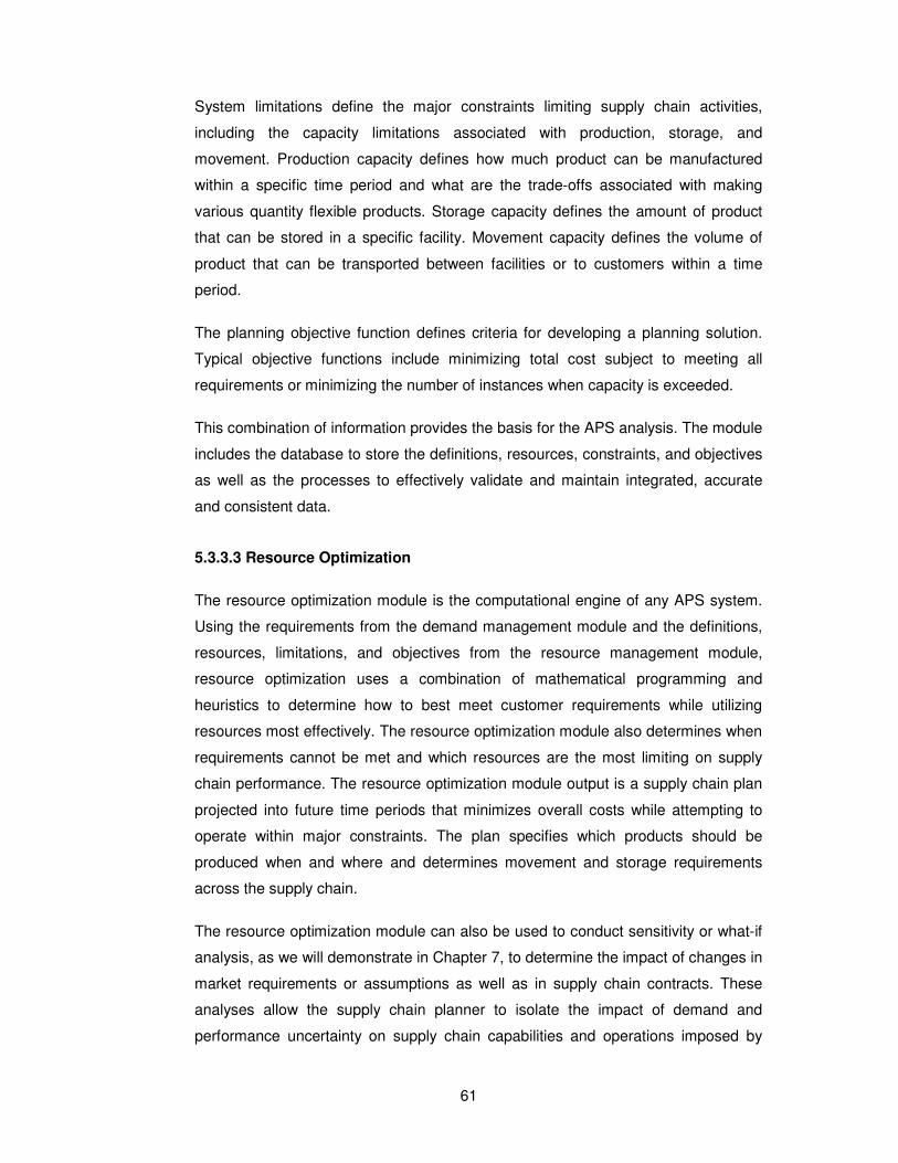
61

System limitations define the major constraints limiting supply chain activities,

including the capacity limitations associated with production, storage, and

movement. Production capacity defines how much product can be manufactured

within a specific time period and what are the trade-offs associated with making

various quantity flexible products. Storage capacity defines the amount of product

that can be stored in a specific facility. Movement capacity defines the volume of

product that can be transported between facilities or to customers within a time

period.

The planning objective function defines criteria for developing a planning solution.

Typical objective functions include minimizing total cost subject to meeting all

requirements or minimizing the number of instances when capacity is exceeded.

This combination of information provides the basis for the APS analysis. The module

includes the database to store the definitions, resources, constraints, and objectives

as well as the processes to effectively validate and maintain integrated, accurate

and consistent data.

5.3.3.3 Resource Optimization

The resource optimization module is the computational engine of any APS system.

Using the requirements from the demand management module and the definitions,

resources, limitations, and objectives from the resource management module,

resource optimization uses a combination of mathematical programming and

heuristics to determine how to best meet customer requirements while utilizing

resources most effectively. The resource optimization module also determines when

requirements cannot be met and which resources are the most limiting on supply

chain performance. The resource optimization module output is a supply chain plan

projected into future time periods that minimizes overall costs while attempting to

operate within major constraints. The plan specifies which products should be

produced when and where and determines movement and storage requirements

across the supply chain.

The resource optimization module can also be used to conduct sensitivity or what-if

analysis, as we will demonstrate in Chapter 7, to determine the impact of changes in

market requirements or assumptions as well as in supply chain contracts. These

analyses allow the supply chain planner to isolate the impact of demand and

performance uncertainty on supply chain capabilities and operations imposed by

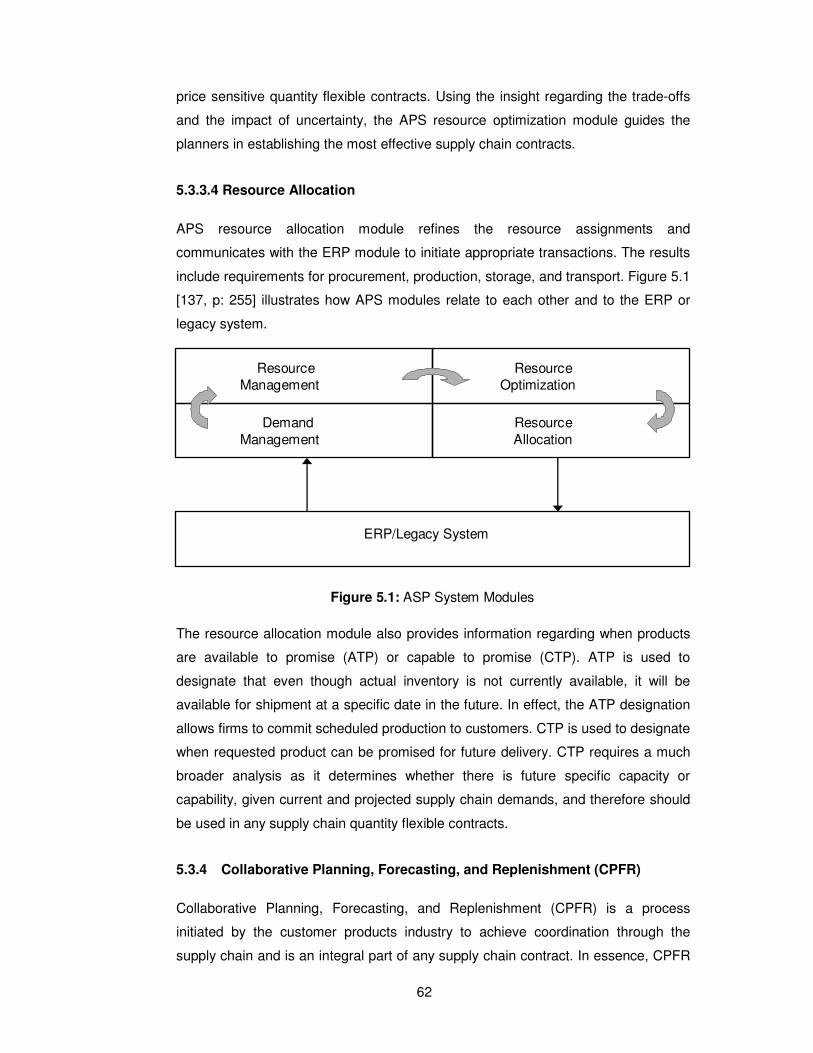
62

price sensitive quantity flexible contracts. Using the insight regarding the trade-offs

and the impact of uncertainty, the APS resource optimization module guides the

planners in establishing the most effective supply chain contracts.

5.3.3.4 Resource Allocation

APS resource allocation module refines the resource assignments and

communicates with the ERP module to initiate appropriate transactions. The results

include requirements for procurement, production, storage, and transport. Figure 5.1

[137, p: 255] illustrates how APS modules relate to each other and to the ERP or

legacy system.

The resource allocation module also provides information regarding when products

are available to promise (ATP) or capable to promise (CTP). ATP is used to

designate that even though actual inventory is not currently available, it will be

available for shipment at a specific date in the future. In effect, the ATP designation

allows firms to commit scheduled production to customers. CTP is used to designate

when requested product can be promised for future delivery. CTP requires a much

broader analysis as it determines whether there is future specific capacity or

capability, given current and projected supply chain demands, and therefore should

be used in any supply chain quantity flexible contracts.

5.3.4 Collaborative Planning, Forecasting, and Replenishment (CPFR)

Collaborative Planning, Forecasting, and Replenishment (CPFR) is a process

initiated by the customer products industry to achieve coordination through the

supply chain and is an integral part of any supply chain contract. In essence, CPFR

Resource

Management

ERP/Legacy System

Resource Optimization

Demand Management

Resource Allocation

Figure 5.1: ASP System Modules

63

coordinates the requirements plan for the demand creation and demand fulfillment

activities. The CPFR solution shares information involving promotions, forecasts,

item data, and orders with trading partners. The collaboratively developed

information is then used jointly and iteratively by planners to generate demand,

determine replenishment requirements, match production to demands, and refine

supply chain contracts.

The first step in the CPFR process is joint business planning wherein a retailer and

supplier share, discuss, coordinate, and rationalize their own individual strategies to

create a partnership strategy, thus a supply chain contract. A common sales

forecast is created and shared between retailer and supplier based on shared

knowledge. CPFR includes an iterative process until a consensus is reached. In

Chapter 7, we also developed profit sharing solutions related to the sharing of the

additional supply chain profit thus generated. Using this consensus forecast,

production, replenishment, and shipment plans are developed. The forecast

becomes a commitment by the trading partners in terms of supply chain contracts.

Besides, these alliances and partnerships create long term relationships between

supply chain partners. Figure 5.2 [137, p: 271] illustrates base CPFR relationships

within the supply chain.

Supplier

Promotions

Forecasts

Item Catalog

Orders

EDI

Internet

CPFR Solution

Trading Partner

Trading Partner

Trading Partner

Collaborate

CRM

APS

ERP

Generate demand

Determine rqmts

Make to demand

Figure 5.2: CPFR

Collaborative Planning, Forecasting, and Replenishment

64

5.3.5 APS Benefits and Considerations within the Supply Chain Contracts

Context

From a supply chain contracts point of view, especially for the price sensitive

quantity flexible model we developed in Chapter 7, there are three broad benefits

that accrue from APS utilization. These include responsiveness to changes,

comprehensive perspective, and resource utilization.

Historically, logistics and supply chain managers have used extended lead times

and schedule freezes to plan for future supply chain activity. The long lead times

and freeze periods were necessary since the planning process was complex and

required substantial analyses. The plans had to be defined early and then frozen to

allow the firm time to execute them. While this approach reduced uncertainty, it also

substantially reduced flexibility and responsiveness, thus reducing the supply chain

surplus.

Today’s customers requires more responsiveness to market needs, and demand for

lower inventory levels rules out long cycle times. Marketplace and firm changes can

be quickly made in the demand management and resource management modules,

allowing for the planning process to use the most current and accurate information.

The requirements optimization module, where the model we developed in Chapter 7

can be part of, then solves the allocation, allowing short term planning cycles rather

than long term. APS thus results in a planning process that can be much more

responsive to marketplace or firm changes.

Second, effective supply chain management requires planning and coordination

across the supply chain. The process must consider the trade-offs associated with

shifting activities, resources, and inventories across organizations. Such a

comprehensive perspective increases planning process complexity substantially.

The complexity follows from the number of organizations, facilities, products, and

assets that must be considered when coordinating activities and resources across

an entire supply chain. APS offers the capability to consider a comprehensive

perspective and make the appropriate trade-offs to achieve optimal supply chain

performance.

Third, APS typically results in substantial supply chain performance improvements in

line with the main objective of maximizing the supply chain performance of supply

chain contracts. While more comprehensive planning and reduced uncertainty

usually result in improved customer service, the major APS benefit is enhanced

65

resource utilization and common objectives. More effective and responsive planning

allows a more even assignment of requirements to existing sourcing, production,

storage, and transportation capacity. The result is that existing capacity is used

more effectively within the supply chain contracts constraints. APS can also

significantly reduce asset requirements by smoothing resource demands. The

decreases include reductions in plant, equipment, facilities, and inventory.

While comprehensive APS is a relatively new capability, the future outlook is bright

as the technology and capacity to effectively evaluate and manage integrated supply

chains are developed. APS can take a comprehensive and dynamic perspective of

the entire supply chain and focus on maximizing the supply chain surplus. Thus, it is

our belief that the models we developed in Chapter 7 can and should be an integral

part of any APS system.

66

CHAPTER 6. SUPPLY CHAIN CONTRACTS AND COMMITTED DELIVERY

STRATEGIES

The strategic fit requires that a company achieve the balance between

responsiveness and efficiency in its supply chain that best meets the needs of the

company’s competitive strategy. The drivers of supply chain performance not only

determine its performance in terms of responsiveness and efficiency, they also

determine whether strategic fit is achieved across the supply chain. In Chapter 4, we

analyzed the impact of inventory, transportation, facilities, and information as the

drivers of supply chain performance. In this chapter, we will analyze supply chain

contracts and their role in maximizing the total supply chain surplus.

Contracts specify the parameters within which a buyer places orders and a supplier

fulfills them. By entering into such a contract, the buyer often stands to gain

guaranteed delivery of the product, which is very useful in times of scarcity, shorter

delivery times, lower purchasing price, or a lower safety stock level. The supplier will

also benefit with a better production plan, reduced variance of demand, economies

of scale, or less paperwork. Harder to measure, but also important, is the increased

level of trust and cooperation which can develop between a buyer and a supplier

who decide to engage in such a contract.

Of particular interest here are contracts that will maximize the total supply chain

surplus.

For simplicity, our supply chain consists of a single manufacturer, a single retailer,

and customers. Transportation costs are included in the wholesale price of the

product, which is assumed at maturity phase of its product life cycle with a normally

distributed constant/horizontal demand pattern. The models can be extended to

more complex supply chains, and/or different demand patterns at different phases of

the product’s life cycle.

This chapter is organized as follows:

In Sections 6.1 and 6.2, we consider a commitment model for a retailer facing price-

sensitive demand and given the opportunity to receive a discount on committed

67

deliveries by using a standard economic model addressed by Lau and Lau [65] and

Thomas [67] that can be viewed as a newsvendor style model. The strength of the

model is the inclusion of demand as a function of the selling price. However, the

model is restricted with the intracompany scope maximizing only the retailer’s profit

without taking into account the total supply chain profit.

In Sections 6.3 to 6.6, we address this weakness of intracompany approach by

introducing the total supply chain surplus with intercompany view, which requires

that both the manufacturer and the retailer evaluate their actions in the context of

the entire supply chain using buyback and quantity flexibility contracts modeled by

Chopra and Meindl [2]. The strength of this model is that both buyback and quantity

flexibility contracts help increase the total supply chain profit. However, there are

two issues that need to be addressed. The first one is related to profit sharing, i.e.,

how to share the additional supply chain surplus thus generated. The second issue,

the main weakness of the contracts discussed, is the fact that demand has not been

correlated to the selling price.

We have used Excel Statistical Functions to evaluate normal distribution functions

used in our numerical experiments. These functions, described in Appendix A, are

then used in a computer program we compiled to find optimum contract parameters

for the model we develop in Chapter 7.

6.1 Retailer Profit without Commitment Opportunity with Demand as a

Function of the Selling Price

Without the opportunity to obtain a discount for commitment, a retailer will seek to

maximize its expected profit π(p) where p is the selling price set by the retailer, c is

the total unit cost (including transportation) and µ(p) is the expected demand as a

function of the selling price. It is assumed that a lower price generates greater

demand so that µ’(p) < 0 and there is no fixed ordering cost. Furthermore, it is also

assumed that the retailer can order any quantity any time during the horizon and

there is no lead time for delivery. The retailer seeks to maximize its expected profit:

maxp π(p) = (p - c) µ(p) (6.1)

Demand functions considered are linear (6.2) and constant elasticity (6.3) demand

functions shown in Figure 6.1 [67].

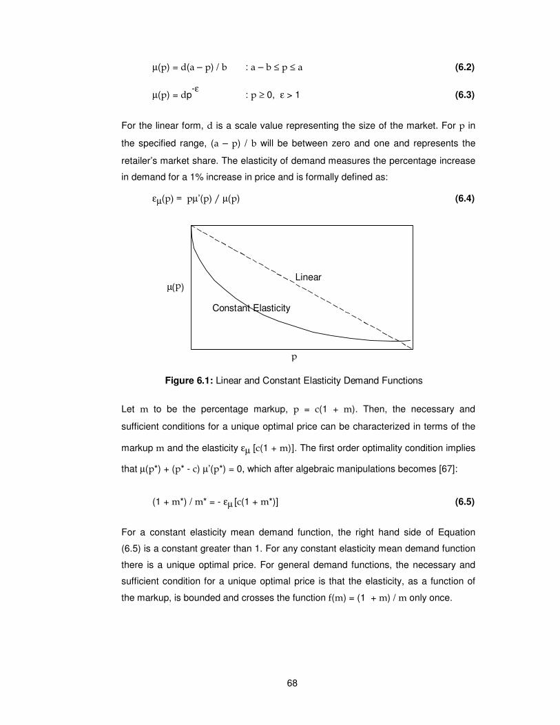
68

µ(p) = d(a – p) / b : a – b ≤ p ≤ a (6.2)

µ(p) = dp-ε

: p ≥ 0, ε > 1 (6.3)

For the linear form, d is a scale value representing the size of the market. For p in

the specified range, (a – p) / b will be between zero and one and represents the

retailer’s market share. The elasticity of demand measures the percentage increase

in demand for a 1% increase in price and is formally defined as:

εµ(p) = pµ’(p) / µ(p) (6.4)

Let m to be the percentage markup, p = c(1 + m). Then, the necessary and

sufficient conditions for a unique optimal price can be characterized in terms of the

markup m and the elasticity εµ [c(1 + m)]. The first order optimality condition implies

that µ(p*) + (p* - c) µ’(p*) = 0, which after algebraic manipulations becomes [67]:

(1 + m*) / m* = - εµ [c(1 + m*)] (6.5)

For a constant elasticity mean demand function, the right hand side of Equation

(6.5) is a constant greater than 1. For any constant elasticity mean demand function

there is a unique optimal price. For general demand functions, the necessary and

sufficient condition for a unique optimal price is that the elasticity, as a function of

the markup, is bounded and crosses the function f(m) = (1 + m) / m only once.

Figure 6.1: Linear and Constant Elasticity Demand Functions

Constant Elasticity

Linear

p

µ ( p )

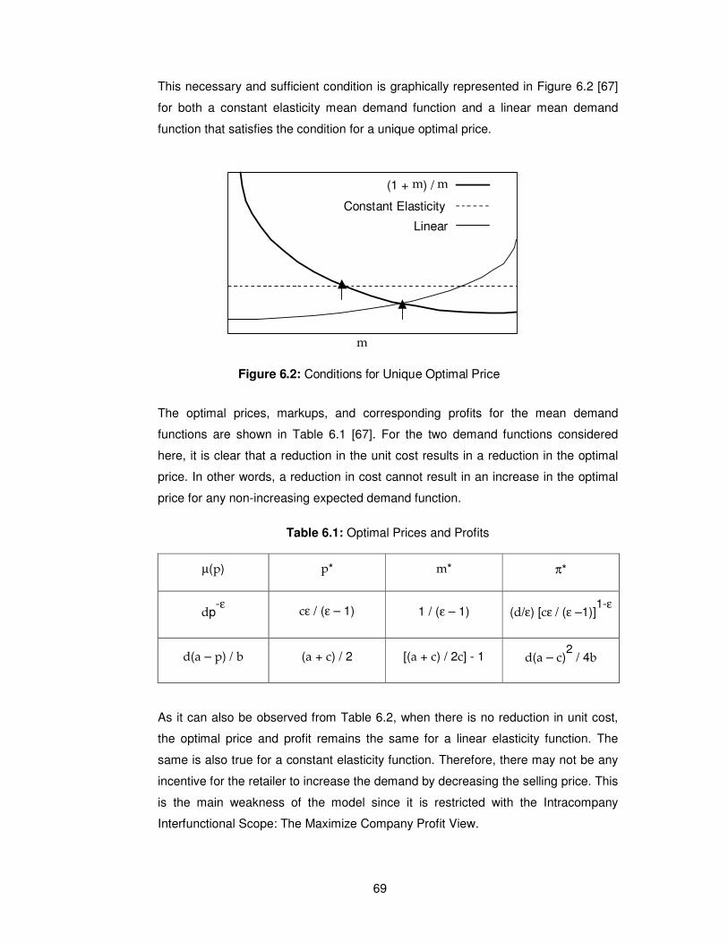
69

This necessary and sufficient condition is graphically represented in Figure 6.2 [67]

for both a constant elasticity mean demand function and a linear mean demand

function that satisfies the condition for a unique optimal price.

The optimal prices, markups, and corresponding profits for the mean demand

functions are shown in Table 6.1 [67]. For the two demand functions considered

here, it is clear that a reduction in the unit cost results in a reduction in the optimal

price. In other words, a reduction in cost cannot result in an increase in the optimal

price for any non-increasing expected demand function.

Table 6.1: Optimal Prices and Profits

µ(p) p* m* π*

dp-ε

cε / (ε – 1) 1 / (ε – 1) (d/ε) [cε / (ε –1)]1-ε

d(a – p) / b (a + c) / 2 [(a + c) / 2c] - 1 d(a – c)2 / 4b

As it can also be observed from Table 6.2, when there is no reduction in unit cost,

the optimal price and profit remains the same for a linear elasticity function. The

same is also true for a constant elasticity function. Therefore, there may not be any

incentive for the retailer to increase the demand by decreasing the selling price. This

is the main weakness of the model since it is restricted with the Intracompany

Interfunctional Scope: The Maximize Company Profit View.

Figure 6.2: Conditions for Unique Optimal Price

Constant Elasticity

Linear

m

(1 + m ) / m

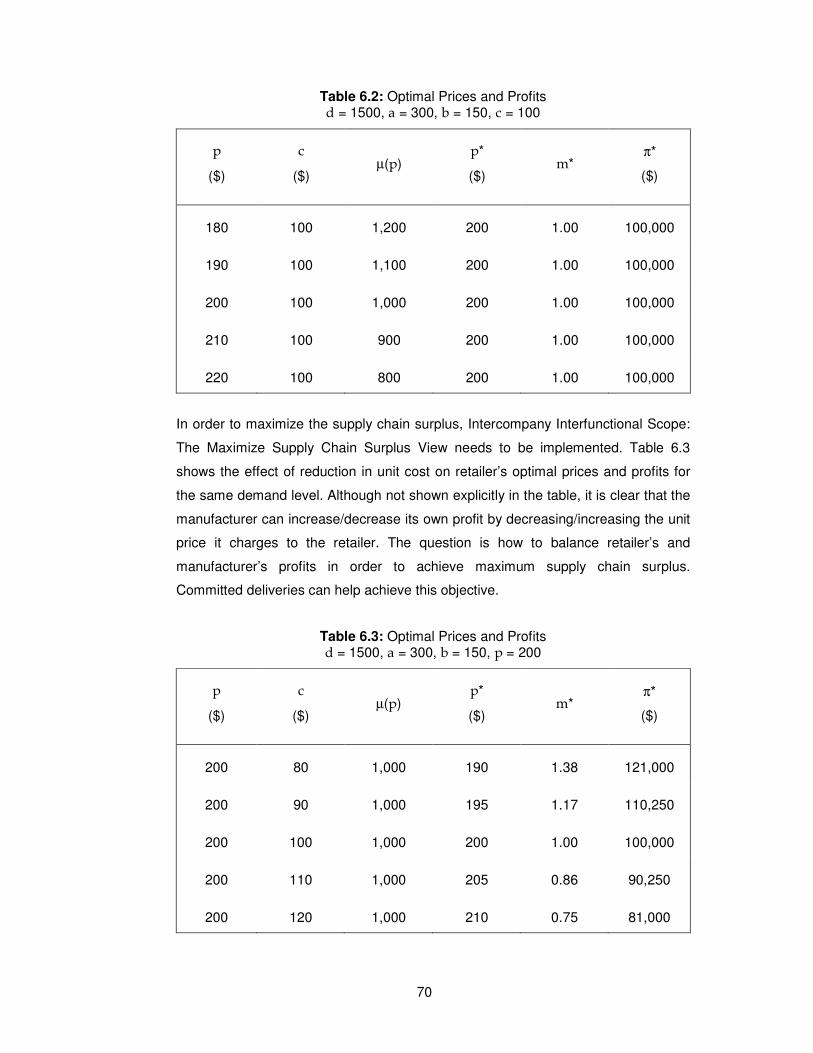
70

Table 6.2: Optimal Prices and Profits d = 1500, a = 300, b = 150, c = 100

p

($)

c

($)

µ(p)

p*

($)

m*

π*

($)

180 100 1,200 200 1.00 100,000

190 100 1,100 200 1.00 100,000

200 100 1,000 200 1.00 100,000

210 100 900 200 1.00 100,000

220 100 800 200 1.00 100,000

In order to maximize the supply chain surplus, Intercompany Interfunctional Scope:

The Maximize Supply Chain Surplus View needs to be implemented. Table 6.3

shows the effect of reduction in unit cost on retailer’s optimal prices and profits for

the same demand level. Although not shown explicitly in the table, it is clear that the

manufacturer can increase/decrease its own profit by decreasing/increasing the unit

price it charges to the retailer. The question is how to balance retailer’s and

manufacturer’s profits in order to achieve maximum supply chain surplus.

Committed deliveries can help achieve this objective.

Table 6.3: Optimal Prices and Profits d = 1500, a = 300, b = 150, p = 200

p

($)

c

($)

µ(p)

p*

($)

m*

π*

($)

200 80 1,000 190 1.38 121,000

200 90 1,000 195 1.17 110,250

200 100 1,000 200 1.00 100,000

200 110 1,000 205 0.86 90,250

200 120 1,000 210 0.75 81,000

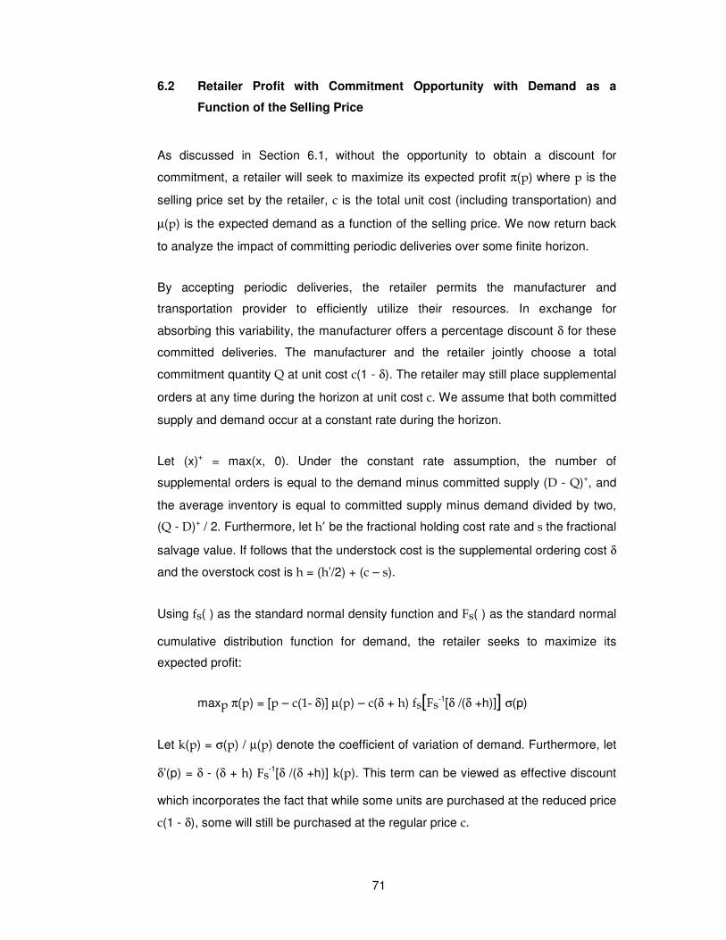
71

6.2 Retailer Profit with Commitment Opportunity with Demand as a

Function of the Selling Price

As discussed in Section 6.1, without the opportunity to obtain a discount for

commitment, a retailer will seek to maximize its expected profit π(p) where p is the

selling price set by the retailer, c is the total unit cost (including transportation) and

µ(p) is the expected demand as a function of the selling price. We now return back

to analyze the impact of committing periodic deliveries over some finite horizon.

By accepting periodic deliveries, the retailer permits the manufacturer and

transportation provider to efficiently utilize their resources. In exchange for

absorbing this variability, the manufacturer offers a percentage discount δ for these

committed deliveries. The manufacturer and the retailer jointly choose a total

commitment quantity Q at unit cost c(1 - δ). The retailer may still place supplemental

orders at any time during the horizon at unit cost c. We assume that both committed

supply and demand occur at a constant rate during the horizon.

Let (x)+ = max(x, 0). Under the constant rate assumption, the number of

supplemental orders is equal to the demand minus committed supply (D - Q)+, and

the average inventory is equal to committed supply minus demand divided by two,

(Q - D)+ / 2. Furthermore, let h’ be the fractional holding cost rate and s the fractional

salvage value. If follows that the understock cost is the supplemental ordering cost δ

and the overstock cost is h = (h’/2) + (c – s).

Using fs( ) as the standard normal density function and Fs( ) as the standard normal

cumulative distribution function for demand, the retailer seeks to maximize its

expected profit:

maxp π(p) = [p – c(1- δ)] µ(p) – c(δ + h) fs[Fs-1[δ /(δ +h)]] σ(p)

Let k(p) = σ(p) / µ(p) denote the coefficient of variation of demand. Furthermore, let

δ’(p) = δ - (δ + h) Fs-1[δ /(δ +h)] k(p). This term can be viewed as effective discount

which incorporates the fact that while some units are purchased at the reduced price

c(1 - δ), some will still be purchased at the regular price c.

72

Therefore, Equation (6.1) where, without the opportunity to obtain a discount for

commitment, a retailer seeks to maximize its expected profit π(p):

maxp π(p) = (p - c) µ(p)

can be written with commitment opportunity as [67]:

maxp π(p) = [p – c[1 – δ’(p)]] µ(p) (6.6)

As it can be observed, commitment will increase expected overstock costs since

flexibility in ordering is reduced, in other words, δ’(p) < δ. Also, the effective per unit

cost falls out even though the discount δ is only given on committed purchases.

Either δ’ > 0 or the retailer is better off not committing.

Commitment strategies can offer market opportunities by contributing to the profit

improvement in two ways: reduction in effective unit cost and improved pricing.

However, it is still restricted with the Intracompany Interfunctional Scope: The

Maximize Company Profit View.

6.2.1 Pricing and Profit Implications of Committed Delivery Strategies

In this section, commitment and pricing decisions associated with different

committed delivery strategies are compared [67]. Constant elasticity expected

demand function µ(p) = dp-ε

with coefficient of variation = 0.3 is used in

calculations performed using Excel. Two cases are considered. In the first case, it is

assumed that the units are fully salvageable at the discounted unit cost s = c(1 - δ)

and that the fractional holding cost rate is h’ = 0.10. Second case is for s = 0.80, and

h’ = 0.10. Figure 6.3 shows the standard commitment level z as a function of δ

where z denotes the optimal fractile of demand, z = Fs-1[δ /(δ +h)].

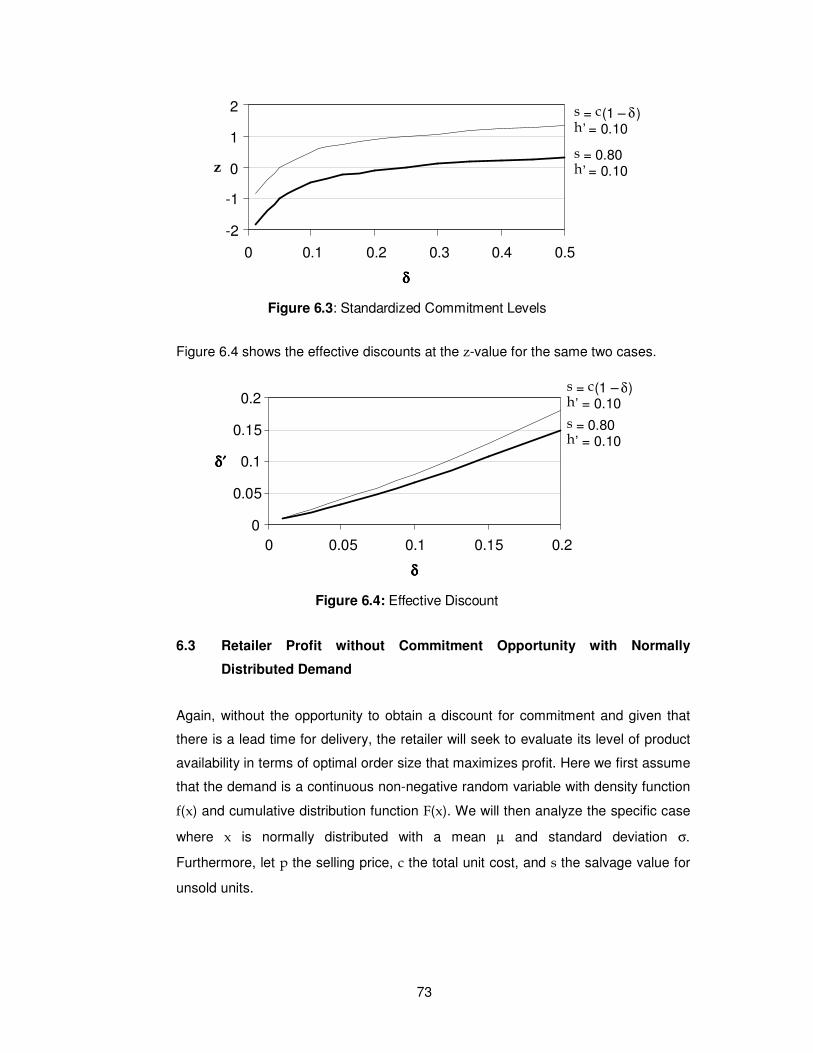
73

Figure 6.4 shows the effective discounts at the z-value for the same two cases.

6.3 Retailer Profit without Commitment Opportunity with Normally

Distributed Demand

Again, without the opportunity to obtain a discount for commitment and given that

there is a lead time for delivery, the retailer will seek to evaluate its level of product

availability in terms of optimal order size that maximizes profit. Here we first assume

that the demand is a continuous non-negative random variable with density function

f(x) and cumulative distribution function F(x). We will then analyze the specific case

where x is normally distributed with a mean µ and standard deviation σ.

Furthermore, let p the selling price, c the total unit cost, and s the salvage value for

unsold units.

Figure 6.3: Standardized Commitment Levels

-2

-1

0

1

2

0 0.1 0.2 0.3 0.4 0.5

δδδδ

z

s = c (1 – δ ) h ’ = 0.10

s = 0.80 h ’ = 0.10

Figure 6.4: Effective Discount

0

0.05

0.1

0.15

0.2

0 0.05 0.1 0.15 0.2

δδδδ

δ′δ′δ′δ′

s = c (1 – δ ) h ’ = 0.10

s = 0.80 h ’ = 0.10

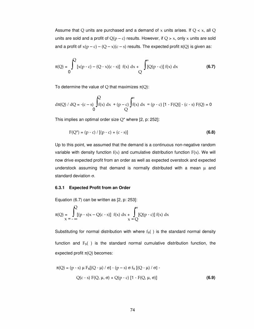
74

Assume that Q units are purchased and a demand of x units arises. If Q < x, all Q

units are sold and a profit of Q(p – c) results. However, if Q > x, only x units are sold

and a profit of x(p – c) – (Q – x)(c – s) results. The expected profit π(Q) is given as:

π(Q) = [x(p - c) – (Q - x)(c - s)] f(x) dx + [Q(p - c)] f(x) dx (6.7)

To determine the value of Q that maximizes π(Q):

dπ(Q) / dQ = -(c – s) f(x) dx + (p – c) f(x) dx = (p - c) [1 - F(Q)] - (c - s) F(Q) = 0

This implies an optimal order size Q* where [2, p: 252]:

F(Q*) = (p - c) / [(p - c) + (c - s)] (6.8)

Up to this point, we assumed that the demand is a continuous non-negative random

variable with density function f(x) and cumulative distribution function F(x). We will

now drive expected profit from an order as well as expected overstock and expected

understock assuming that demand is normally distributed with a mean µ and

standard deviation σ.

6.3.1 Expected Profit from an Order

Equation (6.7) can be written as [2, p: 253]:

π(Q) = [(p - s)x – Q(c - s)] f(x) dx + [Q(p - c)] f(x) dx

Substituting for normal distribution with where fs( ) is the standard normal density

function and Fs( ) is the standard normal cumulative distribution function, the

expected profit π(Q) becomes:

π(Q) = (p - s) µ Fs[(Q - µ) / σ] - (p – s) σ fs [(Q - µ) / σ] -

Q(c - s) F(Q, µ, σ) + Q(p - c) [1 - F(Q, µ, σ)] (6.9)

∫0

Q

∫Q

∞

∫0

Q

∫Q

∞

∫x = - ∞

Q

∫x = Q

∞

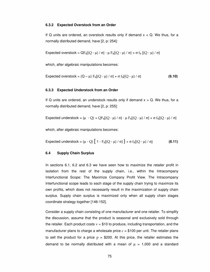
75

6.3.2 Expected Overstock from an Order

If Q units are ordered, an overstock results only if demand x < Q. We thus, for a

normally distributed demand, have [2, p: 254]:

Expected overstock = QFs[(Q - µ) / σ] - µ Fs[(Q - µ) / σ] + σ fs [(Q - µ) / σ]

which, after algebraic manipulations becomes:

Expected overstock = (Q – µ) Fs[(Q - µ) / σ] + σ fs[(Q - µ) / σ] (6.10)

6.3.3 Expected Understock from an Order

If Q units are ordered, an understock results only if demand x > Q. We thus, for a

normally distributed demand, have [2, p: 255]:

Expected understock = (µ - Q) + QFs[(Q - µ) / σ] - µ Fs[(Q - µ) / σ] + σ fs[(Q - µ) / σ]

which, after algebraic manipulations becomes:

Expected understock = (µ - Q) [ 1 - Fs[(Q - µ) / σ] ] + σ fs[(Q - µ) / σ] (6.11)

6.4 Supply Chain Surplus

In sections 6.1, 6.2 and 6.3 we have seen how to maximize the retailer profit in

isolation from the rest of the supply chain, i.e., within the Intracompany

Interfunctional Scope: The Maximize Company Profit View. The Intracompany

Interfunctional scope leads to each stage of the supply chain trying to maximize its

own profits, which does not necessarily result in the maximization of supply chain

surplus. Supply chain surplus is maximized only when all supply chain stages

coordinate strategy together [146-152].

Consider a supply chain consisting of one manufacturer and one retailer. To simplify

the discussion, assume that the product is seasonal and exclusively sold through

the retailer. Each product costs v = $10 to produce, including transportation, and the

manufacturer plans to charge a wholesale price c = $100 per unit. The retailer plans

to sell the product for a price p = $200. At this price, the retailer estimates the

demand to be normally distributed with a mean of µ = 1,000 and a standard

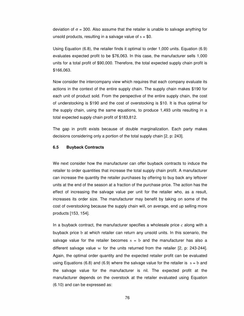
76

deviation of σ = 300. Also assume that the retailer is unable to salvage anything for

unsold products, resulting in a salvage value of s = $0.

Using Equation (6.8), the retailer finds it optimal to order 1,000 units. Equation (6.9)

evaluates expected profit to be $76,063. In this case, the manufacturer sells 1,000

units for a total profit of $90,000. Therefore, the total expected supply chain profit is

$166,063.

Now consider the intercompany view which requires that each company evaluate its

actions in the context of the entire supply chain. The supply chain makes $190 for

each unit of product sold. From the perspective of the entire supply chain, the cost

of understocking is $190 and the cost of overstocking is $10. It is thus optimal for

the supply chain, using the same equations, to produce 1,493 units resulting in a

total expected supply chain profit of $183,812.

The gap in profit exists because of double marginalization. Each party makes

decisions considering only a portion of the total supply chain [2, p: 243].

6.5 Buyback Contracts

We next consider how the manufacturer can offer buyback contracts to induce the

retailer to order quantities that increase the total supply chain profit. A manufacturer

can increase the quantity the retailer purchases by offering to buy back any leftover

units at the end of the season at a fraction of the purchase price. The action has the

effect of increasing the salvage value per unit for the retailer who, as a result,

increases its order size. The manufacturer may benefit by taking on some of the

cost of overstocking because the supply chain will, on average, end up selling more

products [153, 154].

In a buyback contract, the manufacturer specifies a wholesale price c along with a

buyback price b at which retailer can return any unsold units. In this scenario, the

salvage value for the retailer becomes s = b and the manufacturer has also a

different salvage value w for the units returned from the retailer [2, p: 243-244].

Again, the optimal order quantity and the expected retailer profit can be evaluated

using Equations (6.8) and (6.9) where the salvage value for the retailer is s = b and

the salvage value for the manufacturer is nil. The expected profit at the

manufacturer depends on the overstock at the retailer evaluated using Equation

(6.10) and can be expressed as:

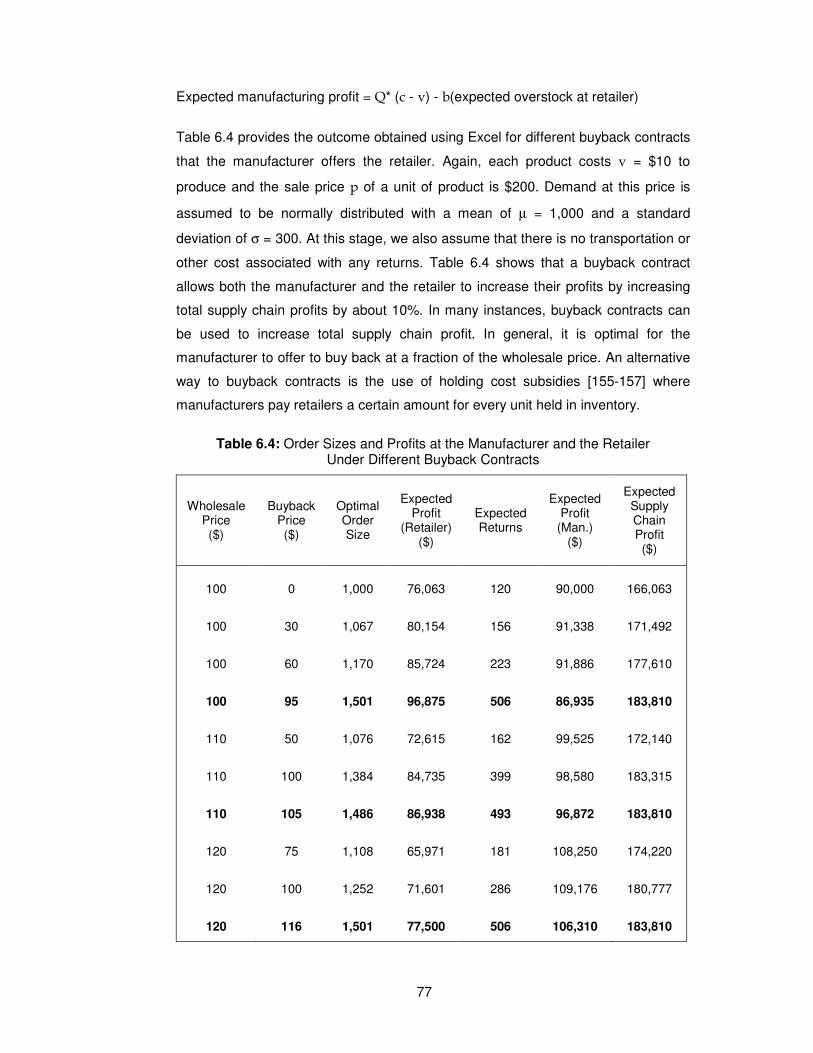
77

Expected manufacturing profit = Q* (c - v) - b(expected overstock at retailer)

Table 6.4 provides the outcome obtained using Excel for different buyback contracts

that the manufacturer offers the retailer. Again, each product costs v = $10 to

produce and the sale price p of a unit of product is $200. Demand at this price is

assumed to be normally distributed with a mean of µ = 1,000 and a standard

deviation of σ = 300. At this stage, we also assume that there is no transportation or

other cost associated with any returns. Table 6.4 shows that a buyback contract

allows both the manufacturer and the retailer to increase their profits by increasing

total supply chain profits by about 10%. In many instances, buyback contracts can

be used to increase total supply chain profit. In general, it is optimal for the

manufacturer to offer to buy back at a fraction of the wholesale price. An alternative

way to buyback contracts is the use of holding cost subsidies [155-157] where

manufacturers pay retailers a certain amount for every unit held in inventory.

Table 6.4: Order Sizes and Profits at the Manufacturer and the Retailer Under Different Buyback Contracts

Wholesale Price ($)

Buyback Price ($)

Optimal Order Size

Expected Profit

(Retailer) ($)

Expected Returns

Expected Profit

(Man.) ($)

Expected Supply Chain Profit ($)

100 0 1,000 76,063 120 90,000 166,063

100 30 1,067 80,154 156 91,338 171,492

100 60 1,170 85,724 223 91,886 177,610

100 95 1,501 96,875 506 86,935 183,810

110 50 1,076 72,615 162 99,525 172,140

110 100 1,384 84,735 399 98,580 183,315

110 105 1,486 86,938 493 96,872 183,810

120 75 1,108 65,971 181 108,250 174,220

120 100 1,252 71,601 286 109,176 180,777

120 116 1,501 77,500 506 106,310 183,810

78

From Table 6.4, it can also be observed that increasing the buyback price always

increases retailer profits and may also increase manufacturer profits. Also, the

manufacturers can increase their profits by increasing the buyback price by a larger

amount than they increase the wholesale price. As an example, the manufacturer

makes a higher profit with a wholesale price of $110 and a buyback price of $100

than it does with a wholesale price of $100 and a buyback price of $60.

It can also be observed that as the wholesale price increases, it is optimal for the

manufacturer to increase the buyback price as well. Another observation is that for a

fixed wholesale price, as the buyback price increases, the retailer orders more and

also returns more. Consequently, as the cost associated with returns increases,

buyback contracts become less attractive because the cost of returns reduces

supply chain profits. In this situation, holding cost subsidies can be used as an

alternative to buyback contracts with similar outcomes.

6.6 Quantity Flexibility Contracts

In quantity flexibility contracts, the manufacturer allows the retailer to change the

quantity ordered after observing demand. If a retailer orders Q units, the

manufacturer commits to providing Q+ = (1 + α)Q units, and the retailer is committed

to buying at least Q- = (1 - β)Q units. Both α and β are between 0 and 1. The retailer

can purchase up to Q+ units depending on the demand observed. These contracts

are similar to buyback contracts in that the manufacturer now bears some of the risk

of having excess inventory. Because no returns are required, these contracts can be

more effective than buyback contracts when the cost of returns is high. Quantity

flexibility contracts increase the average amount the retailer purchases and may

increase total supply chain profits [2, p: 245-246].

As in previous discussions, let v the unit production cost, c the unit wholesale price,

p the unit selling price, s the retailer salvage value, and w the manufacturer salvage

value. The manufacturer produces Q+ units and the retailer purchases Q- units if

demand D is less than Q-, D units if demand D is between Q- and Q+, and Q+ units if

demand D is greater than Q+. We thus obtain:

79

Expected quantity purchased by retailer:

Q = Q- F(Q- ) + Q+ [1 - F(Q+ )] + µ [ Fs[(Q+ - µ) / σ] - Fs[(Q- - µ) / σ]] -

σ [ fs[(Q+ - µ) / σ] - fs[(Q- - µ) / σ]] (6.12)

Expected quantity sold by retailer:

D = Q+ [1 - F(Q+ )] + µ Fs[(Q+ - µ) / σ] - σ fs[(Q

+ - µ) / σ] (6.13)

Expected overstock at manufacturer = Q – D (6.14)

Expected retailer profit = pD + s(Q – D) – cQ (6.15)

Expected manufacturer profit = cQ + w(Q+- Q) -vQ+ (6.16)

Based on the same figures as in the previous examples and using Excel, Table 6.5

provides the impact of different quantity flexibility contracts on supply chain

profitability. All contracts considered are such that the salvage value is nil at both the

manufacturer and the retailer and that α = β.

From Table 6.5 we can observe that quantity flexibility contracts allow both the

manufacturer and the retailer to increase their profits. It is often in the

manufacturer’s best interest to offer a quantity flexibility contract to the retailer. As

an example, for the wholesale price of $100, the manufacturer increases its own

profits by offering a quantity flexibility contract where α and β are equal to 0.2. Total

supply chain profits also increase with quantity flexibility. As the manufacturer

increases the wholesale price, it is optimal to offer greater quantity flexibility to the

retailer.

Vendor-managed Inventories (VMI) is another approach to move the control of the

replenishment decision from the retailer to the manufacturer. VMI can allow a

manufacturer to increase its profits as well as profits for the entire supply chain by

mitigating some of the effects of double marginalization.

.

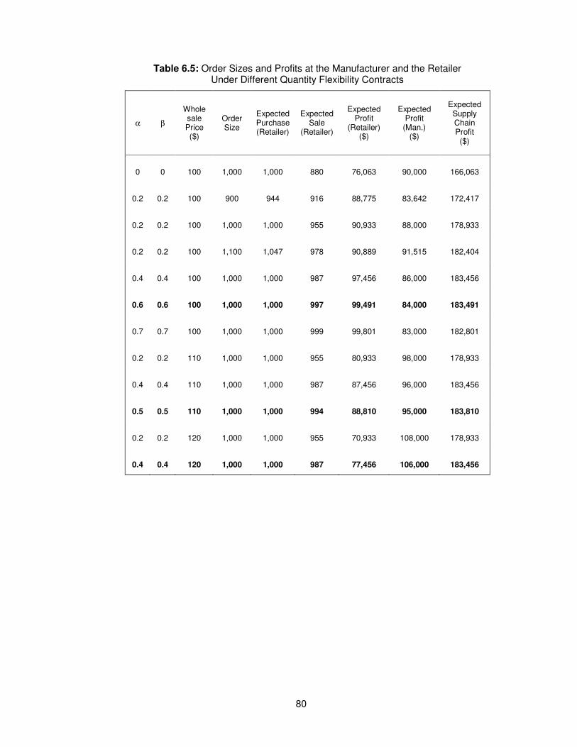
80

Table 6.5: Order Sizes and Profits at the Manufacturer and the Retailer Under Different Quantity Flexibility Contracts

α β

Whole sale Price ($)

Order Size

Expected Purchase (Retailer)

Expected Sale

(Retailer)

Expected Profit

(Retailer) ($)

Expected Profit

(Man.) ($)

Expected Supply Chain Profit ($)

0 0 100 1,000 1,000 880 76,063 90,000 166,063

0.2 0.2 100 900 944 916 88,775 83,642 172,417

0.2 0.2 100 1,000 1,000 955 90,933 88,000 178,933

0.2 0.2 100 1,100 1,047 978 90,889 91,515 182,404

0.4 0.4 100 1,000 1,000 987 97,456 86,000 183,456

0.6 0.6 100 1,000 1,000 997 99,491 84,000 183,491

0.7 0.7 100 1,000 1,000 999 99,801 83,000 182,801

0.2 0.2 110 1,000 1,000 955 80,933 98,000 178,933

0.4 0.4 110 1,000 1,000 987 87,456 96,000 183,456

0.5 0.5 110 1,000 1,000 994 88,810 95,000 183,810

0.2 0.2 120 1,000 1,000 955 70,933 108,000 178,933

0.4 0.4 120 1,000 1,000 987 77,456 106,000 183,456

81

CHAPTER 7. PROPOSED SUPPLY CHAIN CONTRACT MODEL

Both buyback and quantity flexibility contracts help increase the total supply chain

profit. However, there are two issues that need to be addressed. The first one is

related to profit sharing, i.e., how to share the additional supply chain surplus thus

generated. The second issue, the main weakness of the contracts discussed, is the

fact that demand has not been correlated to the selling price. In this chapter we

develop “Maximize Supply Chain Profit with Buyback and Quantity Flexibility

Contracts and Profit Sharing with Demand as a Function of the Selling Price Model”

to address these issues.

This chapter is organized as follows:

In Section 7.1, we analyze and then propose two solutions to address the issue of

profit sharing for quantity flexibility contracts.

In Section 7.2, we develop a model to address the individual weaknesses of the

models discussed by incorporating the price-sensitive demand into quantity flexibility

contracts to maximize the total supply chain profit: Committed Deliveries using

Quantity Flexibility Contracts to Maximize Supply Chain Surplus with Demand as a

Function of the Selling Price.

In Section 7.3, we also develop a computer program to help simulate the system to

find optimum contract parameters for the proposed supply chain contract model.

The program is given in Appendix B.

Finally, in Section 7.4, we compare the existing and proposed models and

emphasize the benefits of using the supply chain contracts with a price-sensitive

demand function and profit sharing as a supply chain performance driver.

7.1 Profit Sharing while Maximizing the Supply Chain Surplus

Table 7.1 partially duplicates Table 6.5 for cases where the wholesale price and

order size are kept constant. As we previously observed, quantity flexibility contracts

allow both the manufacturer and the retailer to increase their profits by increasing

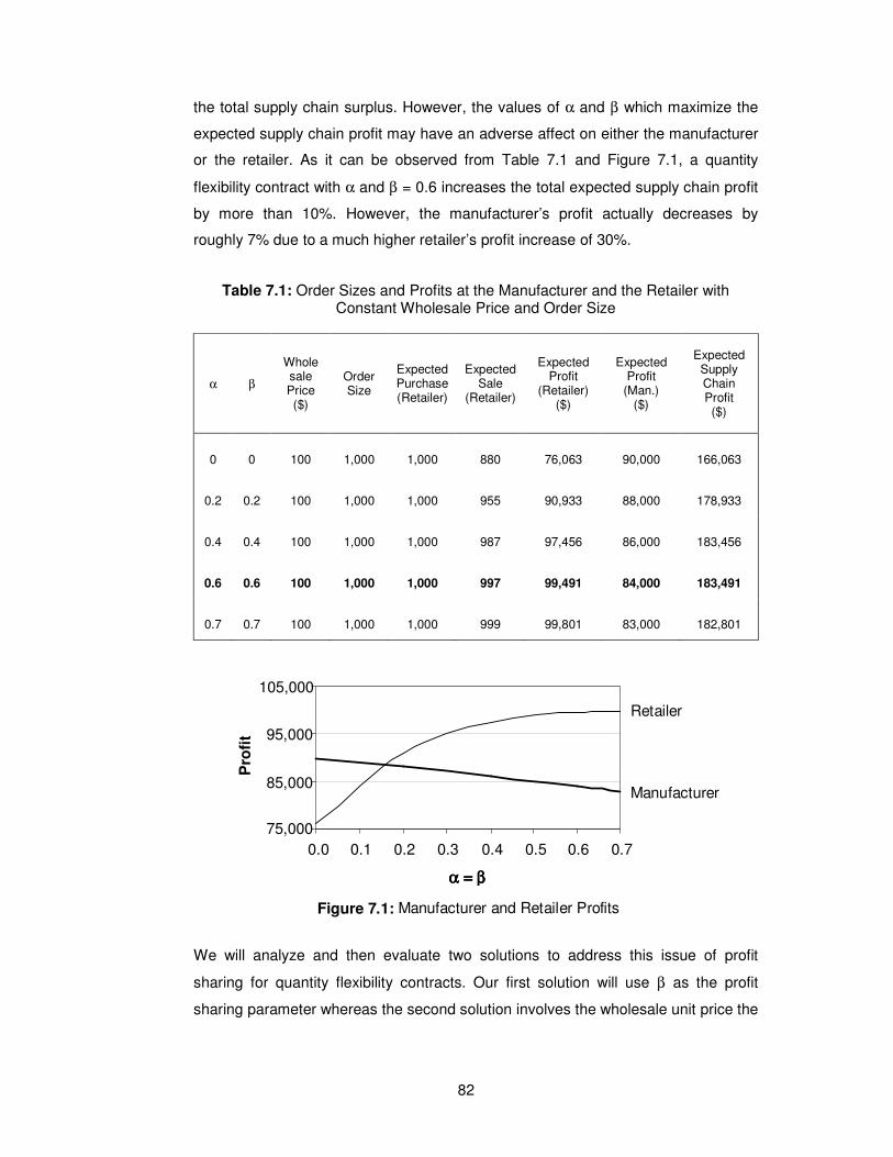
82

the total supply chain surplus. However, the values of α and β which maximize the

expected supply chain profit may have an adverse affect on either the manufacturer

or the retailer. As it can be observed from Table 7.1 and Figure 7.1, a quantity

flexibility contract with α and β = 0.6 increases the total expected supply chain profit

by more than 10%. However, the manufacturer’s profit actually decreases by

roughly 7% due to a much higher retailer’s profit increase of 30%.

Table 7.1: Order Sizes and Profits at the Manufacturer and the Retailer with Constant Wholesale Price and Order Size

α β

Whole sale Price ($)

Order Size

Expected Purchase (Retailer)

Expected Sale

(Retailer)

Expected Profit

(Retailer) ($)

Expected Profit

(Man.) ($)

Expected Supply Chain Profit ($)

0 0 100 1,000 1,000 880 76,063 90,000 166,063

0.2 0.2 100 1,000 1,000 955 90,933 88,000 178,933

0.4 0.4 100 1,000 1,000 987 97,456 86,000 183,456

0.6 0.6 100 1,000 1,000 997 99,491 84,000 183,491

0.7 0.7 100 1,000 1,000 999 99,801 83,000 182,801

We will analyze and then evaluate two solutions to address this issue of profit

sharing for quantity flexibility contracts. Our first solution will use β as the profit

sharing parameter whereas the second solution involves the wholesale unit price the

Figure 7.1: Manufacturer and Retailer Profits

75,000

85,000

95,000

105,000

0.0 0.1 0.2 0.3 0.4 0.5 0.6 0.7

α = βα = βα = βα = β

Pro

fit

Manufacturer

Retailer

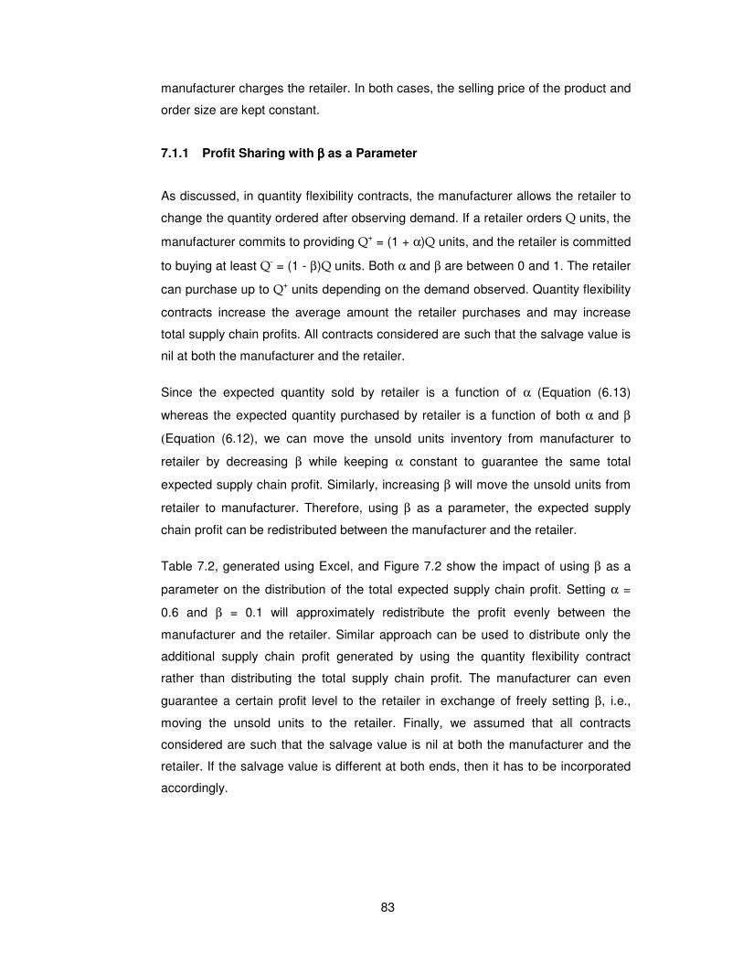
83

manufacturer charges the retailer. In both cases, the selling price of the product and

order size are kept constant.

7.1.1 Profit Sharing with ββββ as a Parameter

As discussed, in quantity flexibility contracts, the manufacturer allows the retailer to

change the quantity ordered after observing demand. If a retailer orders Q units, the

manufacturer commits to providing Q+ = (1 + α)Q units, and the retailer is committed

to buying at least Q- = (1 - β)Q units. Both α and β are between 0 and 1. The retailer

can purchase up to Q+ units depending on the demand observed. Quantity flexibility

contracts increase the average amount the retailer purchases and may increase

total supply chain profits. All contracts considered are such that the salvage value is

nil at both the manufacturer and the retailer.

Since the expected quantity sold by retailer is a function of α (Equation (6.13)

whereas the expected quantity purchased by retailer is a function of both α and β

(Equation (6.12), we can move the unsold units inventory from manufacturer to

retailer by decreasing β while keeping α constant to guarantee the same total

expected supply chain profit. Similarly, increasing β will move the unsold units from

retailer to manufacturer. Therefore, using β as a parameter, the expected supply

chain profit can be redistributed between the manufacturer and the retailer.

Table 7.2, generated using Excel, and Figure 7.2 show the impact of using β as a

parameter on the distribution of the total expected supply chain profit. Setting α =

0.6 and β = 0.1 will approximately redistribute the profit evenly between the

manufacturer and the retailer. Similar approach can be used to distribute only the

additional supply chain profit generated by using the quantity flexibility contract

rather than distributing the total supply chain profit. The manufacturer can even

guarantee a certain profit level to the retailer in exchange of freely setting β, i.e.,

moving the unsold units to the retailer. Finally, we assumed that all contracts

considered are such that the salvage value is nil at both the manufacturer and the

retailer. If the salvage value is different at both ends, then it has to be incorporated

accordingly.

84

Table 7.2: Order Sizes and Profits at the Manufacturer and the Retailer with β as Profit Sharing Parameter

α β

Whole sale Price ($)

Order Size

Expected Purchase (Retailer)

Expected Sale

(Retailer)

Expected Profit

(Retailer) ($)

Expected Profit

(Man.) ($)

Expected Supply Chain Profit ($)

0.6 0.6 100 1,000 1,000 997 99,491 84,000 183,491

0.6 0.4 100 1,000 1,010 997 98,473 85,017 183,491

0.6 0.2 100 1,000 1,043 997 95,212 88,279 183,491

0.6 0.1 100 1,000 1,074 997 92,118 91,372 183,491

0.6 0 100 1,000 1,117 997 87,777 95,714 183,491

7.1.2 Profit Sharing with Wholesale Price as a Parameter

The use of wholesale price as a parameter can also achieve the same profit sharing

objective in a similar way. Wholesale price, being an internal parameter within the

manufacturing and/or replenishment cycle of the supply chain, has no effect on the

total expected supply chain profit. It merely redistributes the total supply chain

surplus between the manufacturer and the retailer. Table 7.3, generated using

Excel, and Figure 7.3 show the impact of using the wholesale price as a parameter

on the distribution of the total expected supply chain profit. Setting the wholesale

price around $108 will approximately redistribute the profit evenly between the

manufacturer and the retailer. Again, similar approach can be used to distribute only

Figure 7.2: Manufacturer and Retailer Profits α = 0.6

75,000

85,000

95,000

105,000

0.0 0.1 0.2 0.3 0.4 0.5 0.6

ββββ

Pro

fit

Manufacturer

Retailer

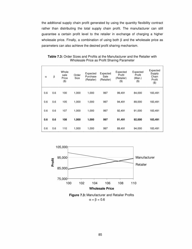
85

the additional supply chain profit generated by using the quantity flexibility contract

rather than distributing the total supply chain profit. The manufacturer can still

guarantee a certain profit level to the retailer in exchange of charging a higher

wholesale price. Finally, a combination of using both β and the wholesale price as

parameters can also achieve the desired profit sharing mechanism.

Table 7.3: Order Sizes and Profits at the Manufacturer and the Retailer with Wholesale Price as Profit Sharing Parameter

α β

Whole sale Price ($)

Order Size

Expected Purchase (Retailer)

Expected Sale

(Retailer)

Expected Profit

(Retailer) ($)

Expected Profit

(Man.) ($)

Expected Supply Chain Profit ($)

0.6 0.6 100 1,000 1,000 997 99,491 84,000 183,491

0.6 0.6 105 1,000 1,000 997 94,491 89,000 183,491

0.6 0.6 107 1,000 1,000 997 92,491 91,000 183,491

0.6 0.6 108 1,000 1,000 997 91,491 92,000 183,491

0.6 0.6 110 1,000 1,000 997 89,491 94,000 183,491

Figure 7.3: Manufacturer and Retailer Profits

α = β = 0.6

75,000

85,000

95,000

105,000

100 102 104 106 108 110

Wholesale Price

Pro

fit Manufacturer

Retailer

86

7.2 Committed Deliveries using Quantity Flexibility Contracts to Maximize

Supply Chain Surplus with Demand as a Function of the Selling Price

We have so far seen that commitment strategies where demand is a function of the

selling price can improve retailer’s profit but are restricted with the Intracompany

Interfunctional Scope: The Maximize Company Profit View. The Intracompany

Interfunctional scope leads to each stage of the supply chain trying to maximize its

own profits, which does not necessarily result in the maximization of supply chain

surplus. Supply chain surplus is maximized only when all supply chain stages

coordinate strategy together. On the other hand, we have also seen that the

Intercompany Interfunctional Scope: The Maximize Supply Chain Surplus View

which requires that each company evaluate its actions in the context of the entire

supply chain can be achieved using buyback or quantity flexibility contracts and

profit sharing where demand is normally distributed, but not a function of the selling

price. Therefore both methodologies are limited in their respective scopes.

Combining both methodologies, we will now develop a model for committed

deliveries using quantity flexibility contracts to maximize supply chain surplus with

demand as a function of the selling price.

As previously discussed, in quantity flexibility contracts, the manufacturer allows the

retailer to change the quantity ordered after observing demand. If a retailer orders Q

units, the manufacturer commits to providing Q+ = (1 + α)Q units, and the retailer is

committed to buying at least Q- = (1 - β)Q units. Both α and β are between 0 and 1.

Furthermore, let again v the unit production cost, c the unit wholesale price, p the

unit selling price, s the retailer salvage value, and w the manufacturer salvage

value. The manufacturer produces Q+ units and the retailer purchases Q- units if

demand D is less than Q-, D units if demand D is between Q- and Q+, and Q+ units if

demand D id greater than Q+ where the demand D is a function of the selling price

with linear elasticity defined as:

D = µ(p) = d(a – p) / b : a – b ≤ p ≤ a (7.1)

We also assume that demand is again normally distributed with a mean µ(p) and

standard deviation σ(p).

Substituting µ(p) and σ(p) into Equations (6.12) to (6.16), we obtain:

87

Expected quantity purchased by retailer:

Q = Q- F(Q- ) + Q+ [1 - F(Q+ )] +

µ(p) [ Fs[(Q+ - µ(p)) / σ(p)] - Fs[(Q- - µ(p)) / σ(p)]] -

σ(p) [ fs[(Q+ - µ(p)) / σ(p)] - fs[(Q- - µ(p)) / σ(p)]] (7.2)

Expected quantity sold by retailer:

D = Q+ [1 - F(Q+ )] + µ(p) Fs[(Q+ - µ(p)) / σ(p)] - σ(p) fs[(Q

+ - µ(p)) / σ(p)] (7.3)

Expected overstock at manufacturer = Q – D (7.4)

Expected retailer profit = pD + s(Q – D) – cQ (7.5)

Expected manufacturer profit = cQ + w(Q+- Q) -vQ+ (7.6)

Based on the same figures as in the previous examples, Tables 7.4 to 7.7,

generated using Excel, show the impact of different quantity flexibility contracts on

supply chain profitability where the demand is a function of the selling price. All

contracts considered are such that the salvage value is nil at both the manufacturer

and the retailer.

Again, let each product costs v = $10 to produce, including transportation, and the

manufacturer plans to charge a wholesale price c = $100 per unit. For consistency

and comparison, we will also use the same linear elasticity function parameters, i.e.,

d = 1500, a = 300, b = 150, and for simplicity let σ(p) = 300 constant.

Table 7.4 and Figure 7.4 show the impact of selling price on the expected supply

chain profit with α = β = 0.6 for a selling price range of $180 to $220.

Since demand is now treated as a function of the selling price, by lowering the

selling price, the supply chain can expect a higher demand and potentially higher

expected supply chain profit. Although the retailer’s expected profit is maximized for

a selling price of $200 when the wholesale price is $100 (as previously shown in

Table 6.3), for the range of values considered, the supply chain’s surplus is

maximized when the selling price is set to $180. The increase in expected sales

(from 997 to 1,199) offsets the decrease in selling price (from $200 to $180) with a

net increase of expected supply chain profit of approximately 7%.

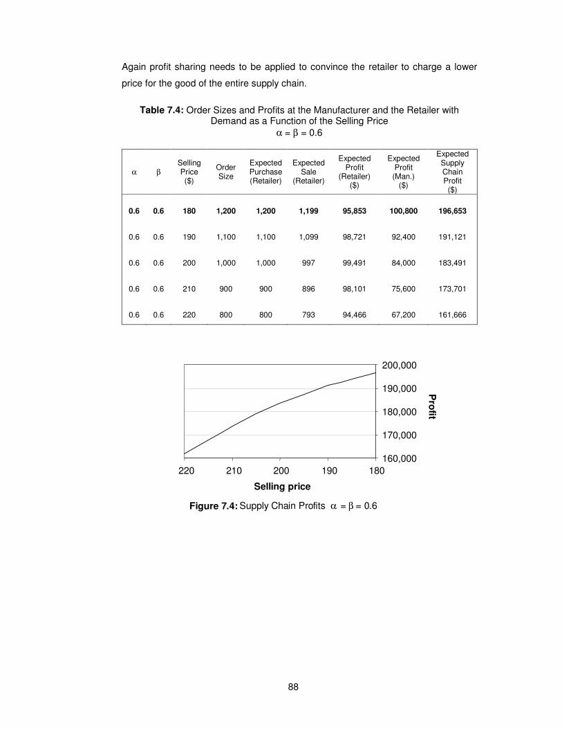
88

Again profit sharing needs to be applied to convince the retailer to charge a lower

price for the good of the entire supply chain.

Table 7.4: Order Sizes and Profits at the Manufacturer and the Retailer with Demand as a Function of the Selling Price

α = β = 0.6

α β Selling Price ($)

Order Size

Expected Purchase (Retailer)

Expected Sale

(Retailer)

Expected Profit

(Retailer) ($)

Expected Profit

(Man.) ($)

Expected Supply Chain Profit ($)

0.6 0.6 180 1,200 1,200 1,199 95,853 100,800 196,653

0.6 0.6 190 1,100 1,100 1,099 98,721 92,400 191,121

0.6 0.6 200 1,000 1,000 997 99,491 84,000 183,491

0.6 0.6 210 900 900 896 98,101 75,600 173,701

0.6 0.6 220 800 800 793 94,466 67,200 161,666

Figure 7.4: Supply Chain Profits α = β = 0.6

160,000

170,000

180,000

190,000

200,000

180 190 200 210 220

Selling price

Pro

fit

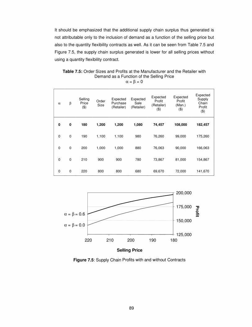
89

It should be emphasized that the additional supply chain surplus thus generated is

not attributable only to the inclusion of demand as a function of the selling price but

also to the quantity flexibility contracts as well. As it can be seen from Table 7.5 and

Figure 7.5, the supply chain surplus generated is lower for all selling prices without

using a quantity flexibility contract.

Table 7.5: Order Sizes and Profits at the Manufacturer and the Retailer with Demand as a Function of the Selling Price

α = β = 0

α β Selling Price ($)

Order Size

Expected Purchase (Retailer)

Expected Sale

(Retailer)

Expected Profit

(Retailer) ($)

Expected Profit

(Man.) ($)

Expected Supply Chain Profit ($)

0 0 180 1,200 1,200 1,080 74,457 108,000 182,457

0 0 190 1,100 1,100 980 76,260 99,000 175,260

0 0 200 1,000 1,000 880 76,063 90,000 166,063

0 0 210 900 900 780 73,867 81,000 154,867

0 0 220 800 800 680 69,670 72,000 141,670

Figure 7.5: Supply Chain Profits with and without Contracts

125,000

150,000

175,000

200,000

180 190 200 210 220

Selling Price

Pro

fit α = β = 0.6

α = β = 0.0

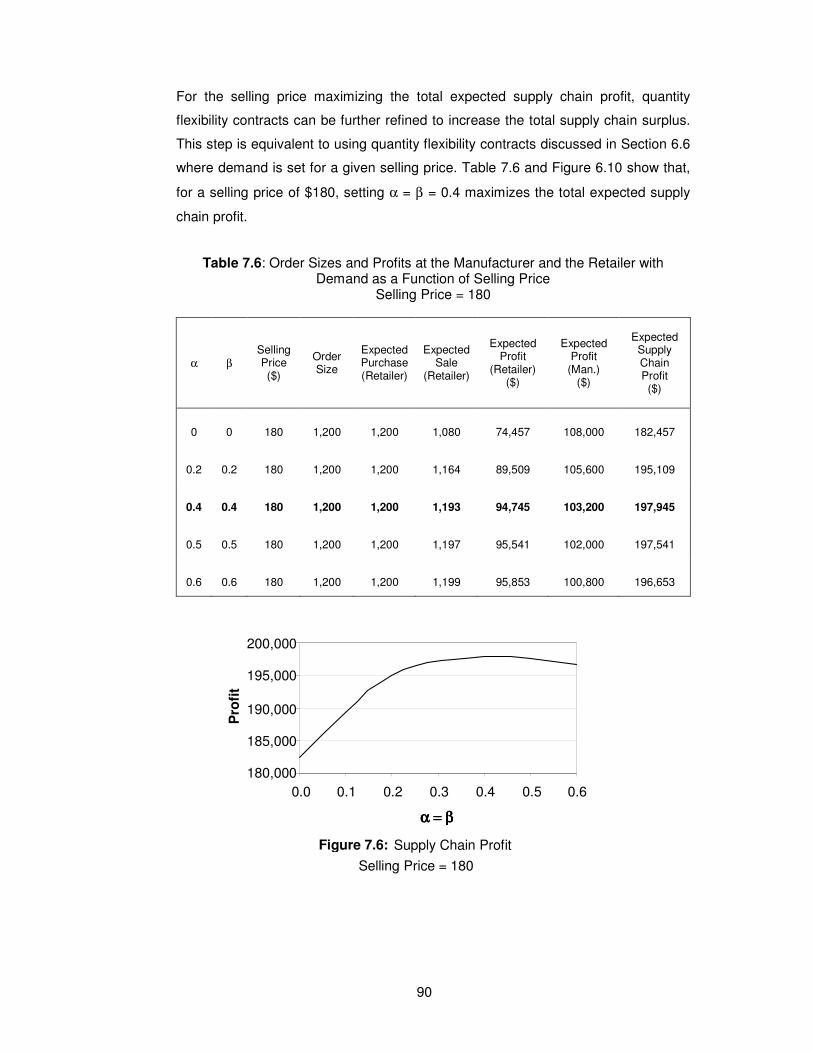
90

For the selling price maximizing the total expected supply chain profit, quantity

flexibility contracts can be further refined to increase the total supply chain surplus.

This step is equivalent to using quantity flexibility contracts discussed in Section 6.6

where demand is set for a given selling price. Table 7.6 and Figure 6.10 show that,

for a selling price of $180, setting α = β = 0.4 maximizes the total expected supply

chain profit.

Table 7.6: Order Sizes and Profits at the Manufacturer and the Retailer with Demand as a Function of Selling Price

Selling Price = 180

α β Selling Price ($)

Order Size

Expected Purchase (Retailer)

Expected Sale

(Retailer)

Expected Profit

(Retailer) ($)

Expected Profit

(Man.) ($)

Expected Supply Chain Profit ($)

0 0 180 1,200 1,200 1,080 74,457 108,000 182,457

0.2 0.2 180 1,200 1,200 1,164 89,509 105,600 195,109

0.4 0.4 180 1,200 1,200 1,193 94,745 103,200 197,945

0.5 0.5 180 1,200 1,200 1,197 95,541 102,000 197,541

0.6 0.6 180 1,200 1,200 1,199 95,853 100,800 196,653

Figure 7.6:

Supply Chain Profit

Selling Price = 180

180,000

185,000

190,000

195,000

200,000

0.0 0.1 0.2 0.3 0.4 0.5 0.6

α = βα = βα = βα = β

Pro

fit

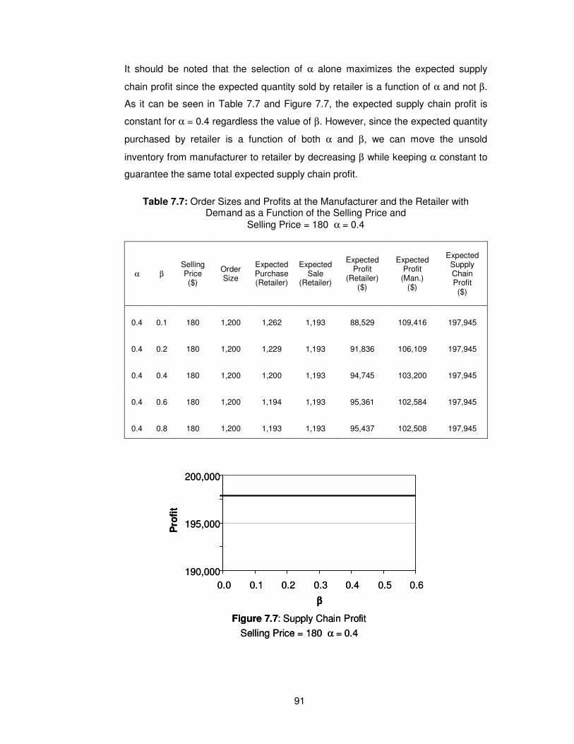
91

It should be noted that the selection of α alone maximizes the expected supply

chain profit since the expected quantity sold by retailer is a function of α and not β.

As it can be seen in Table 7.7 and Figure 7.7, the expected supply chain profit is

constant for α = 0.4 regardless the value of β. However, since the expected quantity

purchased by retailer is a function of both α and β, we can move the unsold

inventory from manufacturer to retailer by decreasing β while keeping α constant to

guarantee the same total expected supply chain profit.

Table 7.7: Order Sizes and Profits at the Manufacturer and the Retailer with Demand as a Function of the Selling Price and

Selling Price = 180 α = 0.4

α β Selling Price ($)

Order Size

Expected Purchase (Retailer)

Expected Sale

(Retailer)

Expected Profit

(Retailer) ($)

Expected Profit

(Man.) ($)

Expected Supply Chain Profit ($)

0.4 0.1 180 1,200 1,262 1,193 88,529 109,416 197,945

0.4 0.2 180 1,200 1,229 1,193 91,836 106,109 197,945

0.4 0.4 180 1,200 1,200 1,193 94,745 103,200 197,945

0.4 0.6 180 1,200 1,194 1,193 95,361 102,584 197,945

0.4 0.8 180 1,200 1,193 1,193 95,437 102,508 197,945

Figure 7.7: Supply Chain Profit

Selling Price = 180 α = 0.4

190,000

195,000

200,000

0.0 0.1 0.2 0.3 0.4 0.5 0.6

β β β β

Pro

fit

Figure 7.7: Supply Chain Profit

Selling Price = 180 α = 0.4

190,000

195,000

200,000

0.0 0.1 0.2 0.3 0.4 0.5 0.6

β β β β

Pro

fit

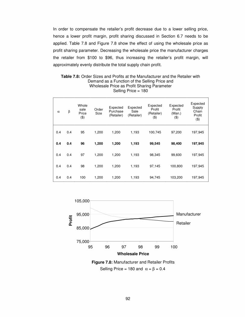
92

In order to compensate the retailer’s profit decrease due to a lower selling price,

hence a lower profit margin, profit sharing discussed in Section 6.7 needs to be

applied. Table 7.8 and Figure 7.8 show the effect of using the wholesale price as

profit sharing parameter. Decreasing the wholesale price the manufacturer charges

the retailer from $100 to $96, thus increasing the retailer’s profit margin, will

approximately evenly distribute the total supply chain profit.

Table 7.8: Order Sizes and Profits at the Manufacturer and the Retailer with Demand as a Function of the Selling Price and Wholesale Price as Profit Sharing Parameter

Selling Price = 180

α β

Whole sale Price ($)

Order Size

Expected Purchase (Retailer)

Expected Sale

(Retailer)

Expected Profit

(Retailer) ($)

Expected Profit

(Man.) ($)

Expected Supply Chain Profit ($)

0.4 0.4 95 1,200 1,200 1,193 100,745 97,200 197,945

0.4 0.4 96 1,200 1,200 1,193 99,545 98,400 197,945

0.4 0.4 97 1,200 1,200 1,193 98,345 99,600 197,945

0.4 0.4 98 1,200 1,200 1,193 97,145 100,800 197,945

0.4 0.4 100 1,200 1,200 1,193 94,745 103,200 197,945

Figure 7.8: Manufacturer and Retailer Profits

Selling Price = 180 and α = β = 0.4

75,000

85,000

95,000

105,000

95 96 97 98 99 100

Wholesale Price

Pro

fit Manufacturer

Retailer

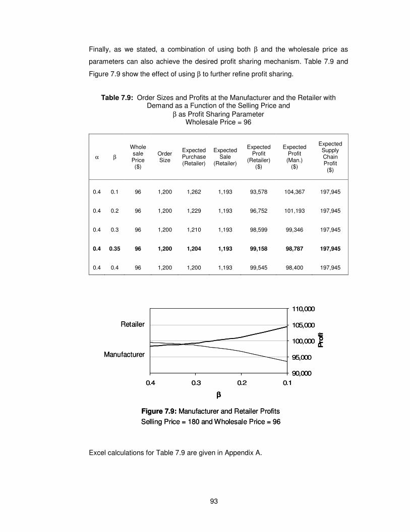
93

Finally, as we stated, a combination of using both β and the wholesale price as

parameters can also achieve the desired profit sharing mechanism. Table 7.9 and

Figure 7.9 show the effect of using β to further refine profit sharing.

Table 7.9: Order Sizes and Profits at the Manufacturer and the Retailer with Demand as a Function of the Selling Price and

β as Profit Sharing Parameter Wholesale Price = 96

α β

Whole sale Price ($)

Order Size

Expected Purchase (Retailer)

Expected Sale

(Retailer)

Expected Profit

(Retailer) ($)

Expected Profit (Man.)

($)

Expected Supply Chain Profit

($)

0.4 0.1 96 1,200 1,262 1,193 93,578 104,367 197,945

0.4 0.2 96 1,200 1,229 1,193 96,752 101,193 197,945

0.4 0.3 96 1,200 1,210 1,193 98,599 99,346 197,945

0.4 0.35 96 1,200 1,204 1,193 99,158 98,787 197,945

0.4 0.4 96 1,200 1,200 1,193 99,545 98,400 197,945

Excel calculations for Table 7.9 are given in Appendix A.

Figure 7.9: Manufacturer and Retailer Profits

Selling Price = 180 and Wholesale Price = 96

90,000

95,000

100,000

105,000

110,000

0.10.20.30.4

ββββ

Pro

fit

Manufacturer

Retailer

Figure 7.9: Manufacturer and Retailer Profits

Selling Price = 180 and Wholesale Price = 96

90,000

95,000

100,000

105,000

110,000

0.10.20.30.4

ββββ

Pro

fit

Manufacturer

Retailer

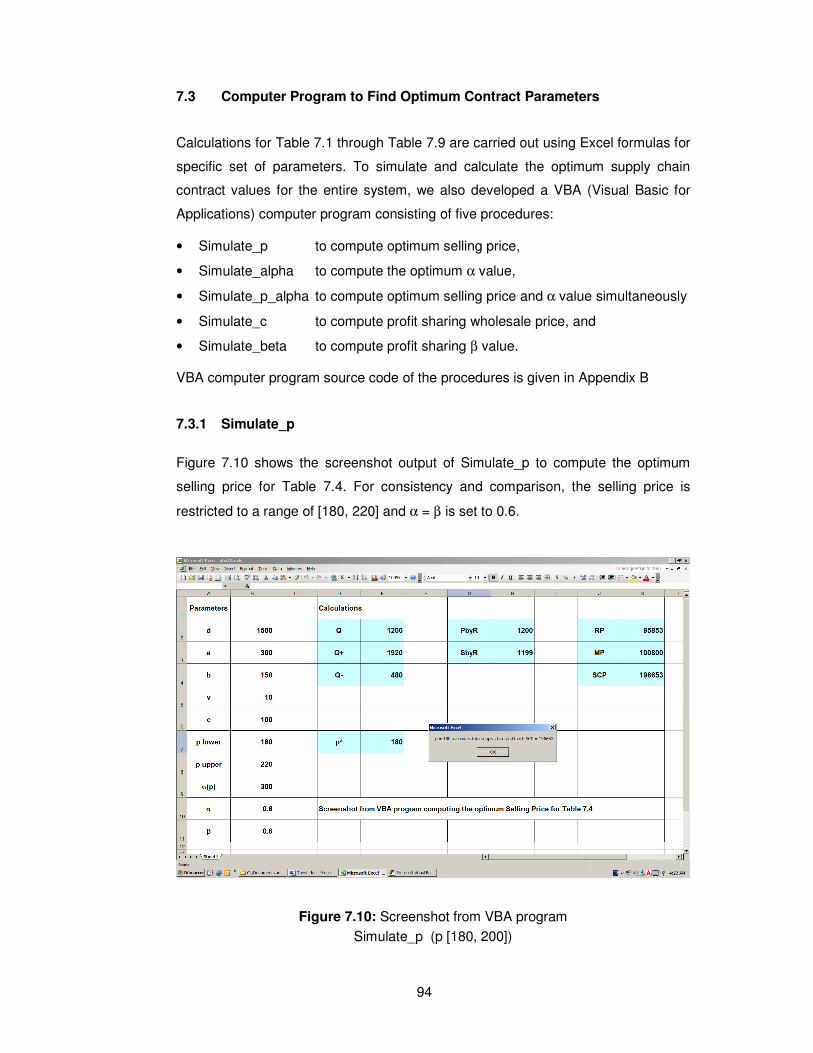
94

7.3 Computer Program to Find Optimum Contract Parameters

Calculations for Table 7.1 through Table 7.9 are carried out using Excel formulas for

specific set of parameters. To simulate and calculate the optimum supply chain

contract values for the entire system, we also developed a VBA (Visual Basic for

Applications) computer program consisting of five procedures:

• Simulate_p to compute optimum selling price,

• Simulate_alpha to compute the optimum α value,

• Simulate_p_alpha to compute optimum selling price and α value simultaneously

• Simulate_c to compute profit sharing wholesale price, and

• Simulate_beta to compute profit sharing β value.

VBA computer program source code of the procedures is given in Appendix B

7.3.1 Simulate_p

Figure 7.10 shows the screenshot output of Simulate_p to compute the optimum

selling price for Table 7.4. For consistency and comparison, the selling price is

restricted to a range of [180, 220] and α = β is set to 0.6.

Figure 7.10: Screenshot from VBA program

Simulate_p (p [180, 200])

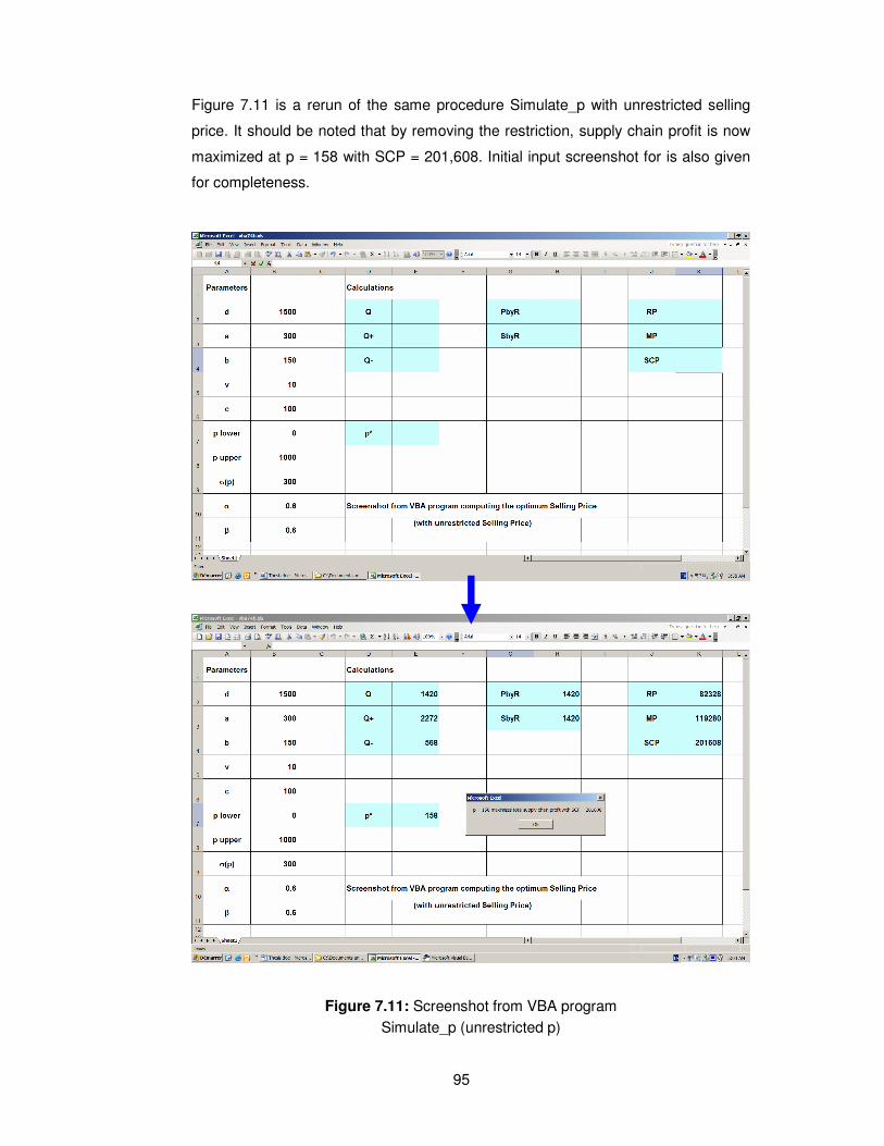
95

Figure 7.11 is a rerun of the same procedure Simulate_p with unrestricted selling

price. It should be noted that by removing the restriction, supply chain profit is now

maximized at p = 158 with SCP = 201,608. Initial input screenshot for is also given

for completeness.

Figure 7.11: Screenshot from VBA program

Simulate_p (unrestricted p)

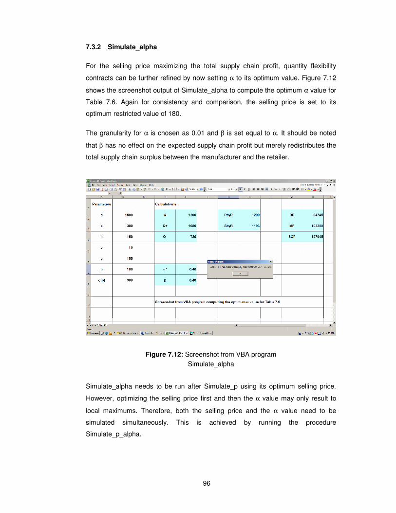
96

7.3.2 Simulate_alpha

For the selling price maximizing the total supply chain profit, quantity flexibility

contracts can be further refined by now setting α to its optimum value. Figure 7.12

shows the screenshot output of Simulate_alpha to compute the optimum α value for

Table 7.6. Again for consistency and comparison, the selling price is set to its

optimum restricted value of 180.

The granularity for α is chosen as 0.01 and β is set equal to α. It should be noted

that β has no effect on the expected supply chain profit but merely redistributes the

total supply chain surplus between the manufacturer and the retailer.

Figure 7.12: Screenshot from VBA program

Simulate_alpha

Simulate_alpha needs to be run after Simulate_p using its optimum selling price.

However, optimizing the selling price first and then the α value may only result to

local maximums. Therefore, both the selling price and the α value need to be

simulated simultaneously. This is achieved by running the procedure

Simulate_p_alpha.

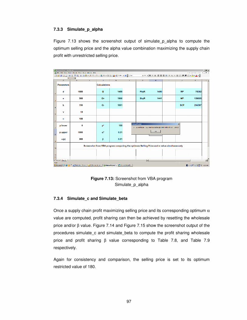
97

7.3.3 Simulate_p_alpha

Figure 7.13 shows the screenshot output of simulate_p_alpha to compute the

optimum selling price and the alpha value combination maximizing the supply chain

profit with unrestricted selling price.

Figure 7.13: Screenshot from VBA program

Simulate_p_alpha

7.3.4 Simulate_c and Simulate_beta

Once a supply chain profit maximizing selling price and its corresponding optimum α

value are computed, profit sharing can then be achieved by resetting the wholesale

price and/or β value. Figure 7.14 and Figure 7.15 show the screenshot output of the

procedures simulate_c and simulate_beta to compute the profit sharing wholesale

price and profit sharing β value corresponding to Table 7.8, and Table 7.9

respectively.

Again for consistency and comparison, the selling price is set to its optimum

restricted value of 180.

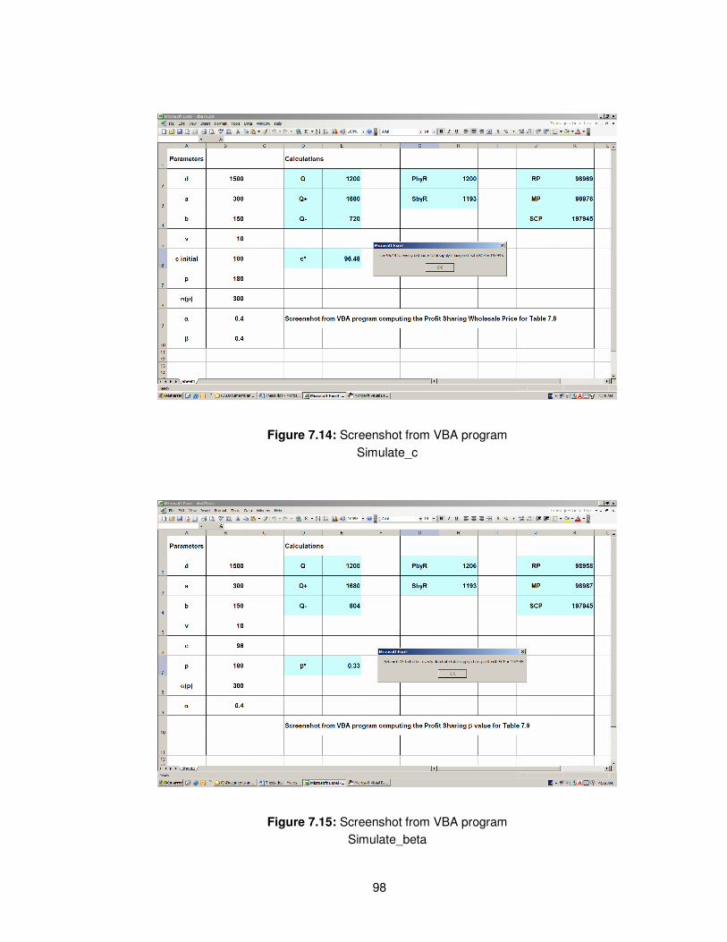
98

Figure 7.14: Screenshot from VBA program

Simulate_c

Figure 7.15: Screenshot from VBA program Simulate_beta

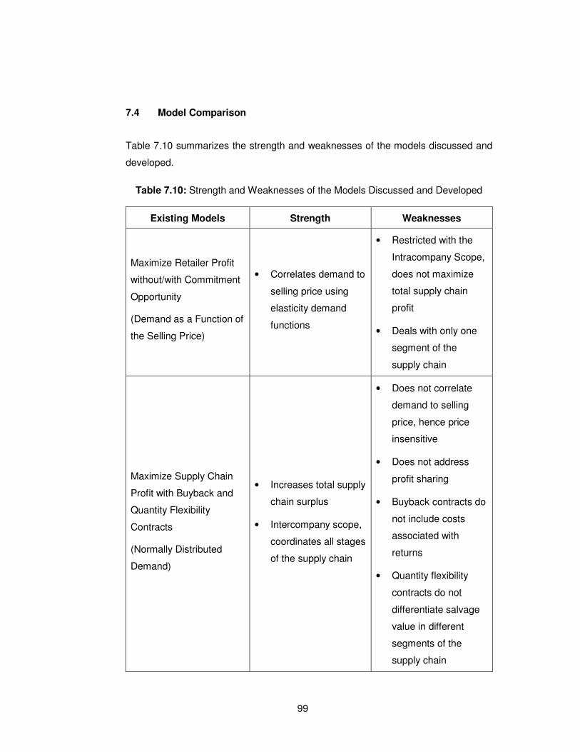
99

7.4 Model Comparison

Table 7.10 summarizes the strength and weaknesses of the models discussed and

developed.

Table 7.10: Strength and Weaknesses of the Models Discussed and Developed

Existing Models Strength Weaknesses

Maximize Retailer Profit

without/with Commitment

Opportunity

(Demand as a Function of

the Selling Price)

• Correlates demand to

selling price using

elasticity demand

functions

• Restricted with the

Intracompany Scope,

does not maximize

total supply chain

profit

• Deals with only one

segment of the

supply chain

Maximize Supply Chain

Profit with Buyback and

Quantity Flexibility

Contracts

(Normally Distributed

Demand)

• Increases total supply

chain surplus

• Intercompany scope,

coordinates all stages

of the supply chain

• Does not correlate

demand to selling

price, hence price

insensitive

• Does not address

profit sharing

• Buyback contracts do

not include costs

associated with

returns

• Quantity flexibility

contracts do not

differentiate salvage

value in different

segments of the

supply chain

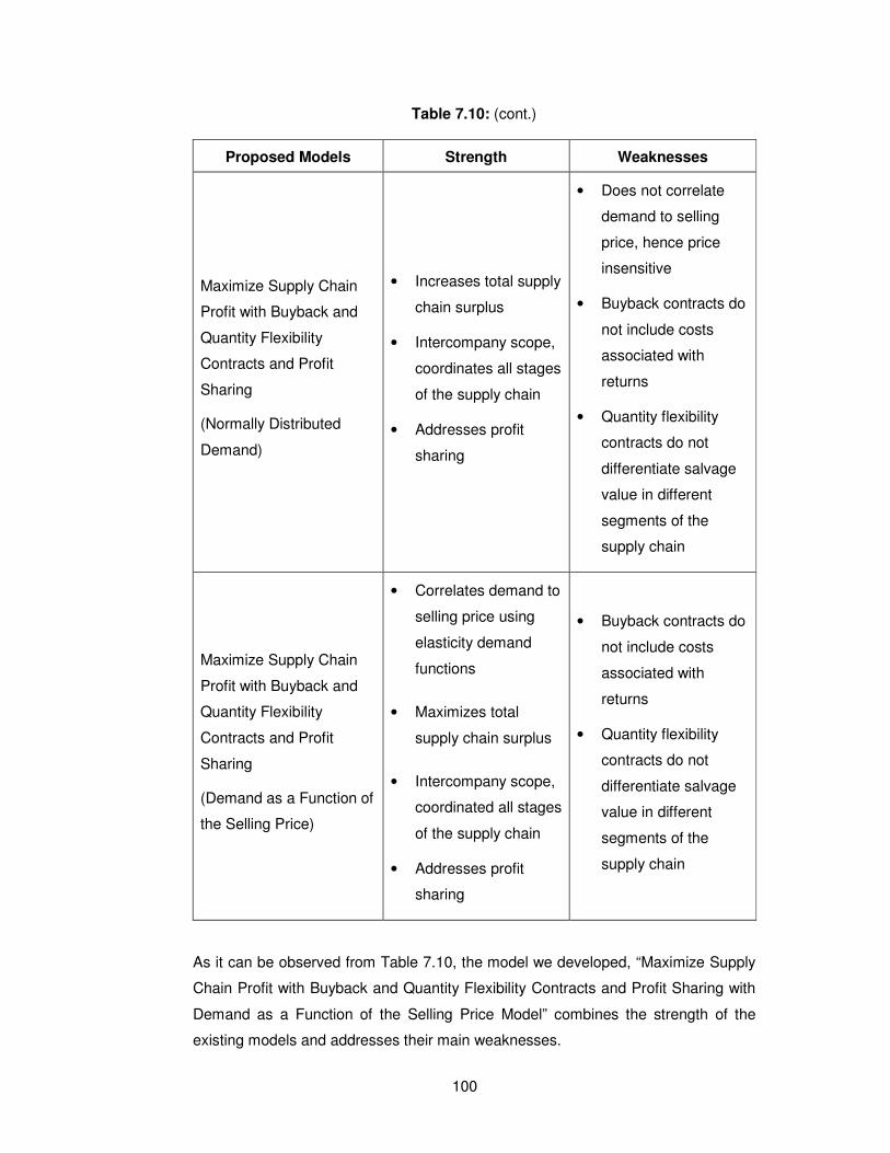
100

Table 7.10: (cont.)

Proposed Models Strength Weaknesses

Maximize Supply Chain

Profit with Buyback and

Quantity Flexibility

Contracts and Profit

Sharing

(Normally Distributed

Demand)

• Increases total supply

chain surplus

• Intercompany scope,

coordinates all stages

of the supply chain

• Addresses profit

sharing

• Does not correlate

demand to selling

price, hence price

insensitive

• Buyback contracts do

not include costs

associated with

returns

• Quantity flexibility

contracts do not

differentiate salvage

value in different

segments of the

supply chain

Maximize Supply Chain

Profit with Buyback and

Quantity Flexibility

Contracts and Profit

Sharing

(Demand as a Function of

the Selling Price)

• Correlates demand to

selling price using

elasticity demand

functions

• Maximizes total

supply chain surplus

• Intercompany scope,

coordinated all stages

of the supply chain

• Addresses profit

sharing

• Buyback contracts do

not include costs

associated with

returns

• Quantity flexibility

contracts do not

differentiate salvage

value in different

segments of the

supply chain

As it can be observed from Table 7.10, the model we developed, “Maximize Supply

Chain Profit with Buyback and Quantity Flexibility Contracts and Profit Sharing with

Demand as a Function of the Selling Price Model” combines the strength of the

existing models and addresses their main weaknesses.

101

CHAPTER 8. CONCLUSIONS AND DIRECTIONS FOR FUTURE RESEACH

In this dissertation we have explored several models addressing the implications of

supply chain contracts in supply chain networks. Our work has focused on the

decisions jointly made by a manufacturer and a retailer to determine the optimal

level of product availability. The central theme in these models has been the notion

of contracts that specify the parameters within which a retailer places orders and a

manufacturer fulfills them in order to maximize the total supply chain surplus.

In Chapter 3, we looked at various supply chain stages, decision phases, cycles,

and supply chain implementation with the objective of maximizing the overall value

generated by the supply chain. In Chapter 4, we reviewed the supply chain

performance in terms of a strategic fit to match supply chain’s responsiveness with

demand uncertainty along with major demand patterns, and the need of an

Intercompany Interfunctional scope to maximize total supply chain surplus. We also

looked at various supply chain drivers to achieve the balance between efficiency

and responsiveness, and obstacles to achieve this strategic fit.

In Chapter 5, we reviewed the impact of information technology structure upon

supply chain collaboration and how APS systems seek to integrate information and

coordinate overall supply chain decisions.

In Chapter 6, we discussed two supply chain contract models. First, where a retailer

facing price sensitive demand may obtain a discount by committing a fixed quantity

over a finite horizon and second where a manufacturer offering buyback or quantity

flexibility contracts may increase the total supply chain profit. We concluded that the

first model incorporates demand as a function of the selling price but does not

address the crucial issue of total supply chain surplus maximization. On the other

hand, the second model, although it increases the total supply chain surplus, does

not incorporate the demand elasticity.

We then developed in Chapter 7 a model to address the individual weaknesses of

the models discussed by incorporating the price sensitive demand into quantity

flexible contracts by determining the optimal level of product availability, as a

function of the selling price, which maximizes the total supply chain profit. We also

102

proposed two solutions to the issue of profit sharing related to the additional supply

chain profit. Furthermore, through numerical experiments, we showed that our

model maximizes total supply chain surplus by incorporating demand elasticity and

profit sharing. We also developed a computer program to help simulate the system

to find optimum contract parameters.

We then summarized the strength and weaknesses of the models discussed with

respect to our model and showed that our model, Maximize Supply Chain Profit with

Buyback and Quantity Flexibility Contracts and Profit Sharing with Demand as a

Function of the Selling Price Model, combines the strength of the models discussed

and addresses their main weaknesses. We strongly believe that the supply chain

contract models developed in this dissertation can be an integral part of any APS

system.

8.1 Future Work

The model presented here assumes that the supply chain consists of a

manufacturer and a retailer. Future work should consider extending the supply chain

to model suppliers and/or distributors as well.

Furthermore, the model assumes that the product is at maturity phase of its life

cycle with a normally distributed constant/horizontal demand pattern. Future work

should consider different demand patterns at different phases of the product’s life

cycle.

Although the model developed addresses major weaknesses of the other models, it

does not include the costs associated with returns in buyback contracts. It does not

differentiate salvage value in different segments of the supply chain for quantity

flexibility contracts either. Future work should also consider addressing these

issues.

For now, the integration of the supply chain contract models developed need to be

implemented into APS software through customized development. The coordination

through the supply chain can then be achieved by Collaborative Planning,

Forecasting, and Replenishment (CPFR) processes. We sincerely believe and hope

to see a supply chain contract module as an integral part of logistical information

systems.

103

BIBLIOGRAPHY

[1] Fredendall, L. and Hill, E., 2001. Basics of Supply Chain Management, St.

Lucie Press, New York.

[2] Chopra, S. and Meindl, P., 2001. Supply Chain Management: Strategy,

Planning, and Operation, Prentice Hall, New Jersey.

[3] Thomas, D. and Griffin, P., 1996. Coordinated Supply Chain Management,

European Journal of Operational Research, 94, 1-15.

[4] Heide, J., 1994. Inter-organizational Governance in Marketing Channels:

Theoretical Perspectives on Forms and Antecedents, Journal of

Marketing, 58(1), 71-85.

[5] Ellinger, A., 2000. Improving Marketing/Logistics Cross-functional Collaboration

in the Supply Chain, Industrial Marketing Management, 29(1), 85-96.

[6] Hagy, K., 2000. Supply Chain Management: Balancing the Organization,

Suppliers and Customer, Pulp & Paper Canada, 101(4), 15-18.

[7] Noordewier, T., John, G., and Nevin, J., 1990. Performance Outcomes of

purchasing arrangements in Industrial Buyer-Vendor Relationships,

Journal of Marketing, 54(10), 80-93.

[8] Buvik, A. and John, G., 1998. When does Vertical Coordination Improve

Industrial Purchasing Relationships?, Working Paper: Carlson School

of Management, University of Minnesota.

[9] Cachon, P. and Fisher, M., 2000. Supply Chain Inventory Management and the

Value of Shared Information, Management Science, 46(8), 1032-

1048.

[10] Chandra, C. and Kumar, S., 2000. Supply Chain Management in Theory and

Practice: A Passing Fad or Fundamental Change, Industrial

Management & Data Systems, 100(3), 100-113.

104

[11] Ballou, R., Gilbert, S., and Mukherjee, A., 2000. New Managerial Challenges

from Supply Chain Opportunities, Industrial Marketing Management,

29(1), 7-18.

[12] Motwani, J., Larson, L., and Ahuja, S., 1998. Managing a Global Supply

Chain Partnership, Logistic Information Management, 11(6), 349-354.

[13] Fox, M., Chionglo, J., and Barbucenau, M., 1993. The Integrated Supply

Chain Management System, Working Paper: Department of Industrial

Engineering, University of Toronto.

[14] Sengupta, S. and Turnbull, J., 1996. Seamless Optimization, IIE Solutions,

October 1996, 28-33.

[15] Humphreys, P., Shiu, W., and Chan, F., 2001. Collaborative Buyer-Supplier

Relationships in Hong Kong Manufacturing Firms, Supply Chain

Management: An International Journal, 6(4), 152-162.

[16] Tracey, M. and Tan, C., 2001. Empirical Analysis of Supplier Selection and

Involvement, Customer Satisfaction, and Firm Performance, Supply

Chain Management: An International Journal, 6(4), 174-188.

[17] Masella, C. and Rangone, A., 2000. A Contingent Approach to the Design of

Vendor Selection Systems for Different Types of Co-operative

Customer/Supplier Relationships, International Journal of Operations

& Production Management, 20(1), 70-84.

[18] Liu, J., Ding, F., and Lall, V., 2000. Using Data Envelopment Analysis to

Compare Suppliers for Supplier Selection and Performance

Improvement, Supply Chain Management: An International Journal,

5(3), 143-150.

[19] Weber, C., Current, J., and Desai, A., 2000. An Optimization Approach to

Determining the Number of Vendors to Employ, Supply Chain

Management: An International Journal, 5(2), 90-98.

[20] Lambert, D., Cooper, M., and Pagh, J., 1998. Supply Chain Management:

Implementation Issues and Research Opportunities, International

Journal of Logistics Management, 9(2), 1-19.

105

[21] Trent, R. and Monczka, R., 1999. Achieving World-class Supplier Quality,

Total Quality Management, 10(6), 927-938.

[22] Milgate, M., 2001. Supply Chain Complexity and Delivery Performance: An

International Exploratory Study, Supply Chain Management: An

International Journal, 6(3), 106-118.

[23] Spina, G. and Zotteri, G., 2001. The Strategic Context of Customer-Supplier

Partnerships: Evidence from a Global Survey, Integrated

Manufacturing Systems, 12(7), 483-492.

[24] Anupindi, R. and Akella, R., 1993. Diversification under Supply Uncertainty,

Management Science, 39(8), 944-963.

[25] Kohli, R. and Park, H., 1994. Coordinating Buyer-Seller Transactions across

Multiple Products, Management Science, 40(9), 45-50.

[26] He, X., Xu, S., Ord, K., and Hayya, J., 1998. An Inventory Model with Order

Crossover, Operations Research, 46(3), 112-119.

[27] Weng, Z., 1995. Channel Coordination and Quantity Discounts, Management

Science, 41(9), 1509-1522.

[28] Weng, Z., 1995. Modeling Quantity Discounts under General Price-sensitive

Demand Functions: Optimal Policies and Relationships, European

Journal of Operational Research, 86, 300-314.

[29] Weng, Z., 1997. Pricing and Ordering Strategies in Manufacturing and

Distribution Alliances, IIE Transactions, 29(8), 681-692.

[30] Rau, H., Wu, M., and Wee, H., 2003. Integrated Inventory Model for

Deteriorating Items under a Multi Echelon Supply Chain Environment,

International Journal of Production Economics, 85(3), 155-168.

[31] Ernst, R. and Pyke, D., 1993. Optimal Base Stock Policies and Truck Capacity

in a Two-Echelon System, Naval Research Logistics, 40, 879-903.

[32] Yano, C. and Gerchak, Y., 1989. Transportation Contracts and Safety Stocks

for Just-In-Time Deliveries, Journal of Manufacturing and Operations

Management, 2, 314-330.

106

[33] Henig, M., Gerchak, Y., Ernst, R., and Pyke, D., 1997. An Inventory Model

Embedded in Designing a Supply Contract, Management Science,

43(2), 184-189.

[34] Bassok, Y. and Anupindi, R., 1997. Analysis of Supply Contracts with Total

Minimum Commitment, IIE Transactions, 29(8), 373-381.

[35] Anupindi, R. and Bassok, Y., 1998. Approximations for Multiproduct Contracts

with Stochastic Demands and Business Volume Discounts, IIE

Transactions, 30(8), 723-734.

[36] Bassok, Y., Bixby, A., Srinivasan, R., and Weisel, H., 1997. Design of

Component Supply Contract with Commitment Revision Flexibility,

IBM Journal of Research and Development, 41(6), 693-703.

[37] Eppen, G. and Iyer, A., 1997. Backup Agreements in Fashion Buying: Value of

Upstream Flexibility, Management Science, 43(11), 1469-1484.

[38] Eppen, G. and Iyer, A., 1997. Improved Fashion Buying with Bayesian

Updates, Operations Research, 45(6), 805-819.

[39] Tsay, A., 1997. The Quantity Flexible Contract and Supplier-Customer

Incentives, Working Paper: Leavey School of Business, Santa Clara

University.

[40] Vargas, V. and Metters, R., 1996. Adapting Lot sizing Techniques to

Stochastic Demand through Production Scheduling Policy, IIE

Transactions, 28(8), 141-148.

[41] Smith, R. and Zhang, R., 1998. Infinite Horizon production Planning in Time

Varying Systems with Convex Production and Inventory Costs,

Management Science, 44(9), 1313-1320.

[42] DeCroix, G. and Arreola-Risa, A., 1998. On Offering Economic Incentives to

Backorder, IIE Transactions, 30(8), 715-721.

[43] Glasserman, P. and Tayur, S., 1995. Sensitivity Analysis for Base Stock

Levels in MultiEchelon Production Inventory Systems, Management

Science, 41(2), 263-281.

107

[44] Lee, H. and Whang, S., 1992. The Quantity Decentralized MultiEchelon

Inventory Control Systems: Incentives and Information, Working

Paper: Standford University.

[45] Ganeshan, R., Boone, T., and Stenger, A., 2001. The Impact of Inventory and

Flow Planning Parameters on Supply Chain Performance: An

Exploratory Study, International Journal of Production Economics, 71,

111-118.

[46] Kapuscinksi, R. and Tayur, S., 1998. Capacitated Production Inventory Model

with Periodic Demand, Operations Research, 46(6), 899-911.

[47] Zipkin, P.,1989. Critical Number Policies for Inventory Models with Periodic

Data, Management Science, 35(1), 71-80.

[48] Moon, C., Kim, J., and Hur, S., 2002. Integrated Process Planning and

Scheduling with Minimizing Total Tardiness in Multi-plants Supply

Chain, Computers and Industrial Engineering, 43(1-2), 331-349.

[49] Timpe, C. and Kallrath, J., 2000. Optimal Planning in Large Multi-site

Production Networks, European Journal of Operational Research,

126, 422-435.

[50] Vergara, F., Khouja, M., and Michalewicz, Z., 2002. An Evolutionary

Algorithm Optimizing Material Flow in Supply Chains, Computers and

Industrial Engineering, 43(3), 407-421.

[51] Chan, F., Tang, N., Lau, H., and Ip, R., 2002. A Simulation Approach in Supply

Chain Management, Integrated Manufacturing Systems, 13(2), 117-

122.

[52] Syarif, A., Yun, Y., and Gen, M., 2002. Study on Multi-stage Logistics Chain

Network: A Spanning Tree-based Genetic Algorithm Approach,

Computers and Industrial Engineering, 43(1-2), 299-314.

[53] Doran, D., 2002. Manufacturing for Synchronous Supply: A Case Study of

Ikeda Hoover Ltd, Integrated Manufacturing Systems, 13(1), 18-24.

108

[54] Min, H. and Guo, Z., 2004. The location of Hub-seaports in the Global Supply

Chain Network Using a Cooperative Competition Strategy, Integrated

Supply Management, 1(1), 51-63.

[55] Han, D., Kwon, I., Bae, M., and Sung, H., 2002. Supply Chain Integration in

Developing Countries for Foreign Retailers in Korea: Wall-Mart

Experience, Computers and Industrial Engineering, 43(1-2), 111-121.

[56] Masters, J., 1993. Determination of Near Optimal Stock Levels for Multi

Echelon Distribution Inventories, Journal of Business Logistics, 14(2),

165-195.

[57] Sox, C. and Muckstadt, J., 1996. Multi-Item, Multi-Period production Planning

with Uncertain Demand, IIE Transactions, 28(11), 891-900.

[58] Moinzadeh, K. and Nahmias, S., 1988. A continuous Review Model for an

Inventory System with Two Supply Modes, Management Science,

34(6), 761-773.

[59] Gurnani, H., 1996. Optimal Ordering Policies in Inventory Systems with

Random Demand and Random Deal Offerings, European Journal of

Operational Research, 95(2), 299-312.

[60] Zheng, Y., 1994. Optimal Control Policy for Stochastic Inventory Systems with

Markovian Discount Opportunities, Operations Research, 42(4), 721-

738.

[61] Moinzadeh, K., 1997. Replenishment and Stocking Policies for Inventory

Systems with Random Deal Offerings, Management Science, 43(3),

334-342.

[62] Ritchken, P. and Tapiero, C., 1998. Contingent Claims Contracting for

Purchasing Decisions in Inventory Management, Operations

Research, 34(6), 864-870.

[63] Kohli, R. and Park, H., 1989. A Cooperative Game Theory Model of Quantity

Discounts, Management Science, 35(6), 693-707.

109

[64] Gallego, G. and Moon, I., 1993. The Distribution –free newsboy Problem:

Review and Extensions, Journal of the Operational Research

Society, 44, 825-834.

[65] Lau, A. and Lau, H., 1997. The Distribution-free newsboy Problem: Review and

Extensions, European Journal of the Operational Research, 103(3),

557-572.

[66] Khouja, M., 1996. The A Note on the Newsboy Problem with an Emergency

Supply Option, Journal of the Operational Research Society, 47,

1530-1534.

[67] Thomas, D., 1999. Committed Delivery Strategies for Supply Chain

Management, Ph.D. Thesis, Industrial and Systems Engineering,

Georgia Institute of Technology, Georgia.

[68] Barnes-Schuster, C., 1996. Supply Chain Management and the Use of Long

Term Supply Contracts, Ph.D. Thesis, Industrial Engineering and

Management Sciences, NorthWestern University, Illinois.

[69] Fisher, M., 1997. What is the Right supply Chain for Your product?, Harvard

Business Review, March-April 1997, 83-93.

[70] Fuller, J., O’Conner, J., and Rawlinson, R., 1993. Tailored Logistics: The

Next Advantage, Harvard Business Review, May-June 1993, 87-98.

[71] Cox, A., 1999. Power, Value and Supply Chain Management, Supply Chain

Management: An International Journal, 4(4), 167-175.

[72] Desbarats, G., 1999. The Innovation Supply Chain, Supply Chain

Management, 4(1), 7-10.

[73] Lummus, R., Krumwiede, D., and Vokurka, R., 2001. The Relationship of

Logistics to Supply Chain Management: Developing a Common

Industry Definition, Industrial Management & Data Systems, 101(8),

426-431.

[74] Langabeer, J. and Rose, J., 2001. Creating Demand Driven Supply Chains:

How to Profit from Demand Chain Management, Chandos Publishing,

Oxford.

110

[75] Blackwell, R. and Blackwell, K., 1999. The Century of the Customer:

Converting Supply Chains into Demand Chains, Supply Chain

Management Review, Fall 1999, 22-32.

[76] Proud, J., 1999. Master Scheduling: A Practical Guide to Competitive

Manufacturing, John Wiley & Sons, New York.

[77] Bovet, D. and Frentzel, D., 1999. The Value Net: Connecting for Profitable

Growth, Supply Chain Management Review, Fall 1999, 96-104.

[78] Min, H. and Zhou, G., 2002. Supply Chain Modeling: Past, Present and Future,

Computers and Industrial Engineering, 43(1-2), 231-249.

[79] Marien, E., 2000. The Four supply Chain Enablers, Supply Chain Management

Review, March-April 2000, 96-104.

[80] Li, Z., Kumar, A., and Lim, Y., 2002. Supply Chain Modelling: A Coordination

Approach, Integrated Manufacturing Systems, 13(8), 551-561.

[81] Blattberg, R. and Neslin, S., 1990. Sales Promotion: Concepts, Methods, and

Strategies, Prentice-Hall, New Jersey.

[82] Brealey, R. and Myers, S., 2000. Principles of Corporate Finance, Irwin

McGraw-Hill, Boston.

[83] Buzzell, R., Quelch, J., and Salmon, W., 1990. The Costly Bargain of Trade

Promotions, Harvard Business Review, March-April 1990, 141-149.

[84] Federgruen, A. and Zheng, Y., 1993. Optimal Power-of-Two Replenishment

Strategies in Capacitated General Production/Distribution Networks,

Management Science, 39, 710-727.

[85] Silver, E., Pyke, D., and Petersen, R., 1998. Inventory Management and

Production Planning and Scheduling, John Wiley & Sons, New York.

[86] Li, Z., Kumar, A., and Lim, Y., 2002. Supply Chain Modelling: A Coordination

Approach, Integrated Manufacturing Systems, 13(8), 551-561.

[87] Ballou, R., 1999. Business Logistics Management, Prentice-Hall, New Jersey.

[88] Tyworth, J., Cavinato, J., and Langley, C., 1991. Traffic Management:

Planning, Operations, and Control, Waveland Press, Illinois.

111

[89] Robeson, J. and Copacino, W., 1994. The Logistics Handbook, The Free

Press, New York.

[90] Sakawa, M., Nishizaki, I., and Uemura, Y., 2002. A Decentralized Two-level

Transportation Problem in a Housing Material Manufacturer:

Interactive Fuzzy Programming Approach, European Journal of

Operational Research, 141, 167-185.

[91] Narasimhan, A. and Palekar, U., 2002. Analysis and Algorithms for the

Transtainer Routing Problem in Container Port Operations,

Transportation Science, 36(1), 63-78.

[92] Preston, P. and Kozan, E., 2001. An Approach to Determine Storage Location

of Containers at Seaport Terminals, Computers and Operations

Research, 28(10), 983-995.

[93] Kurz, M. and Askin, R., 2003. Comparing Scheduling Rules for Flexible Flow

Lines, International Journal of Production Economics, 85(3), 371-388.

[94] Ferdows, K., 1997. Making the Most of Foreign Factories, Harvard Business

Review, March-April 1997, 73-88.

[95] Lee, Y. and Kim, S., 2002. Production-distribution Planning in Supply Chain

Considering Capacity Constraints, Computers and Industrial

Engineering, 43(1-2), 169-190.

[96] Perry, M. and Sohal, A., 2001. Effective Quick Response Practices in a Supply

Chain Partnership: An Australian Case Study, International Journal of

Operations and Production Management, 21(5/6), 840-854.

[97] Kim, S. and Ha, D., 2003. A JIT Lot Splitting Model for Supply Chain

Management: Enhancing Buyer-Supplier Linkage, International

Journal of Production Economics, 85(3), 1-10.

[98] Zhou, G., Min, H., and Gen, M., 2003. A Genetic Algorithm Approach to the Bi-

criteria Allocation of Customers to Warehouses, International Journal

of Production Economics, 85(3), 33-45.

[99] Philip, E. and Wurster, T., 1999. Getting Real About Virtual Commerce,

Harvard Business Review, November-December 1999, 84-94.

112

[100] Kehoe, D. and Boughton, N., 2001. Internet based Supply Chain

Management: A Classification of Approaches to Manufacturing

Planning and Control, International Journal of Operations &

Production Management, 21(4), 516-524.

[101] Lancioni, R., Smith M., and Olivia T., 2000. The Role of the Internet in

Supply Chain Management, Industrial Marketing Management, 29(1),

45-56.

[102] Rao, B., 1999. The Internet and The Revolution in Distribution: A Cross

Industry Examination, Technology in Society, 21, 287-306.

[103] Nurmilaakso, J., Kettunen, J., and Seilonen, I., 2002. XML Based Supply

Chain Integration: A Case Study, Integrated Manufacturing Systems,

13(8), 586-595.

[104] Shim, S., Pendyala, V., Sundaram, M., and Gao, J., 2000. Business-to-

Business e-commerce Frameworks, IEEE Computer, 33(10), 40-47.

[105] Wu, I., 2003. Understanding Senior Management’s Behaviour in Promoting the

Strategic Role of IT in Process Reengineering: Use of the Theory of

Reasoned Action, Information & Management, 41(2), 1-13.

[106] Calosso, T., Cantamessa, M., Vu, D., and Villa, A., 2003. Production

Planning and Order Acceptance in Business to Business Electronic

Commerce, International Journal of Production Economics, 85(3),

233-249.

[107] Irani, Z., Themistocleous, M., and Love, P., 2003. The Impact of Enterprise

Application Integration on Information System Lifecycles, Information

& Management, 41(2), 177-187.

[108] Byrd, T. and Davidson, N., 2003. Examining Possible Antecedents of IT

Impact on the Supply Chain and its Effects on Firm Performance,

Information & Management, 41(2), 243-255.

[109] Lee, S. and Lim, G., 2003. The Impact of Partnership Attributes on EDI

Implementation Success, Information & Management, 41(2), 135-

148.

113

[110] Doll, W., Deng, Z., and Scazzero, J., 2003. A Process for Post

Implementation IT Benchmarking, Information & Management, 41(2),

199-212.

[111] Dellaert, N. and Jeunet, J., 2003. Controlling Multi Level Production in a

Rolling Schedule Environment, International Journal of Production

Economics, 85(3), 113-121.

[112] Arakawa, M., Fuyuki, M., and Inoue, I., 2003. An Optimization Oriented

Method for Simulation Based Job Shop Scheduling Incorporating

Capacity Adjustment Function, International Journal of Production

Economics, 85(3), 359-369.

[113] Wilding, R., 1998. The Supply Chain Complexity Triangle: Uncertainty

Generation in the Supply Chain, International Journal of Physical

Distribution & Logistics Management, 28(8), 599-616.

[114] Haughton, M. and Stenger, A., 1999. Comparing Strategies for Addressing

Delivery Shortages in Stochastic Demand Settings, Transportation

Research Part E, 35, 25-41.

[115] Lau, A. and Lau, H., 2002. The effects of Reducing Demand Uncertainty in a

Manufacturer-retailer Channel for Single Period Products, Computers

and Operations Research, 29, 1583-1602.

[116] Petrovic, D., 2001. Simulation of Supply Chain Behaviour and Performance in

an Uncertain Environment, International Journal of Production

Economics, 71, 429-438.

[117] Power, D., Rahman, S., and Sohal, A., 2001. Critical Success Factors in

Agile Supply Chain Management, International Journal of Physical

Distribution & Logistics Management, 31(4), 247-265.

[118] Christopher, M., 2000. The Agile Supply Chain: Competing in Volatile

Markets, Industrial Marketing Management, 29(1), 37-44.

[119] Kaufman, A., Wood, C., and Theyel, G., 2000. Collaboration and Technology

Linkages: A Strategic Supplier Typology, Strategic Management

Journal, 21(6), 649-663.

114

[120] Lancioni, R., 2000. New Developments in Supply Chain Management for the

Millennium, Industrial Marketing Management, 29(1), 1-6.

[121] Schonsleben, P., 2000. With Agility and Adequate Partnership Strategies

towards Effective Logistic Networks, Computers in Industry, 42(1),

33-42.

[122] Wadhwa, S. and Rao, K., 2000. Flexibility: An Emerging Meta-competence for

Managing High Technology, International Journal of Technology

Management, 19(8), 820-845.

[123] Zhang, Z. and Sharifi, H., 2000. A Methodology for Achieving Agility in

Manufacturing Organizations, International Journal of Operations &

Production Management, 20(4), 496-512.

[124] Yusuf, Y., Gunasekaran, A., Adeleye, E., and Sivayoganathan, K., 2003.

Agile Supply Chain Capabilities: Determinants of Competitive

Objectives, European Journal of Operational Research, 2003.

[125] Gunasekaran, A. and Yusuf, Y., 2002. Agile Manufacturing: A Taxonomy of

Strategic and Technological Imperatives, International Journal of

Production Research, 40(6), 1357-1385.

[126] Hoek, R., Harrison, A., and Christopher, M., 2001. Measuring Agile

Capabilities in the Supply Chain, International Journal of Operations

and Production Management, 21(1/2), 126-147.

[127] Prince, J. and Kay, J., 2003. Combining Lean and Agile Characteristics:

Creation of Virtual Groups by Enhanced Production Flow Analysis,

International Journal of Production Economics, 85(3), 305-318.

[128] Barad, M. and Sapir, E., 2003. Flexibility in Logistic Systems: Modeling and

Performance Evaluation, International Journal of Production

Economics, 85(3), 155-170.

[129] Birgün Barla, S., 2003. A Case Study of Supplier Selection for Lean Supply

by Using a Mathematical Model, Logistics Information Management,

16(6), 451-459.

115

[130] Lancioni, R., Forman H., and Smith, M., 2001. Logistics and Supply Chain

Education, International Journal of Physical Distribution & Logistics

Management, 31(10), 733-745.

[131] Stratton, R. and Warburton, R., 2003. The Strategic Integration of Agile and

Lean Supply, International Journal of Production Economics, 85(3),

183-198.

[132] Gordon, J. and Sohal, A., 2001. Assessing Manufacturing Plant

Competitiveness, International Journal of Operations and Production

Management, 21(1/2), 233-253.

[133] Gibson, B. and Cook, R., 2001. Hiring Practices in US third-party Logistics

Firms, International Journal of Physical Distribution & Logistics

Management, 31(10), 714-732.

[134] Aitken, J., Childerhouse, P., and Towill, D., 2003. The Impact of Product

Life Cycle on Supply Chain Strategy, International Journal of

Production Economics, 85(3), 127-140.

[135] Arkader, R., 2001. The Perspective of Suppliers on Lean Supply in a

Developing Country Context, Integrated Manufacturing Systems,

12(2), 87-93.

[136] Gunasekaran, A., 2001. Agile Manufacturing: The 21st Century Competitive

Strategy, Elsevier Science Ltd., Oxford.

[137] Bowersox, D., Closs D., Cooper M., 2002. Supply Chain Logistics

Management, McGraw-Hill, New York.

[138] Cunningham, J., Dean F., Stevens G., 2001. Implementing Oracle Financial

Analyzer, Addison-Wesley, Harlow.

[139] Beamon, B., 1999. Measuring Supply Chain Performance, International

Journal of Operations & Production Management, 19(3), 275-292.

[140] Korpela, J., Lehmusvaara, A., and Tuominen, M., 2001. Customer Service

Based Design of the Supply Chain, International Journal of

Production Economics, 69(2), 193-204.

116

[141] Lee, Y., Gen, M., and Hochbaum, D., 2002. A Focused Issue on Supply

Chain Management, Computers and Industrial Engineering, 43(1-2),

1-3.

[142] Beard, J. and Sumner, M., 2004. Seeking Strategic Advantage in the Post-

net Era: Viewing ERP Systems from the Resource-based

Perspective, Journal of Strategic Information Systems, 13, 129-150.

[143] Brown, C. and Vessey, I., 2003. Managing the Next Wave of Enterprise

Systems: Leveraging lessons from ERP, MIS Quarterly Executive, 2,

65-77.

[144] Holland, C. and Light, B., 2001. A Stage Maturity Model for Enterprise

Resource Planning Systems Use, Database for Advances in

Information Systems, 35, 34-45.

[145] Sumner, M., 2005. Enterprise Resource Planning, Prentice Hall, New Jersey.

[146] Clark, T. and Hammond, J., 1997. Reengineering Channel Reordering

Processes to Improve Total Supply Chain Performance, Production

and Operations Management, 6, 266-276.

[147] Fisher, M., Hammond, J., Obermeyer, W., and Raman, A., 1994. Making

Supply Meet Demand in an Uncertain World, Harvard Business

Review, May-June 1994, 83-93.

[148] Disney, S. and Towill, R., 2003. The Effect of Vendor Managed Inventory

(VMI) Dynamics on the Bullwhip Effect in Supply Chains,

International Journal of Production Economics, 85(3), 199-215.

[149] Khouja, M. and Robbins, S., 2003. Linking Advertising and Quantity

Decisions in the Single Period Inventory Model, International Journal

of Production Economics, 85(3), 93-105.

[150] Lee, Y., Cho, M., Kim, S., and Kim, Y., 2002. Supply Chain Simulation with

Discrete-continuous Combined Modeling, Computers and Industrial

Engineering, 43(3), 375-392.

117

[151] So, K. and Zheng, X., 2003. Impact of Supplier’s Lead Time and Forecast

Demand Updating on Retailer’s Order Quantity Variability in a Two

Level Supply Chain, International Journal of Production Economics,

85(3), 169-179.

[152] Salameh, M., Abboud, N., El-Kassar, N., and Ghattas, R., 2003.

Continuous Review Inventory Model with Delay in Payments,

International Journal of Production Economics, 85(3), 91-95.

[153] Gulati, R. and Singh, H., 1998. The Architecture of Cooperation: Managing

Coordination Costs and Appropriation Concerns in Strategic

Alliances, Administrative Science Quarterly, (43), 781-814.

[154] Boyson, S. and Thomas, C., 2001. The Real Time Supply Chain, Sloan

Management Review, Spring 1992, 65-73.

[155] Lee, H. and Billington, C., 1992. Managing Supply Chain Inventory, Supply

Chain Management Review, January-February 2001, 44-50.

[156] Padmanabhan, V. and Png, I., 1995. Return Policies: Making Money by

Making Good, Sloan Management Review, Fall 1995, 65-72.

[157] Kumar, N., 1996. The Power of Trust in Manufacturer-Retailer Relationships,

Harvard Business Review, November-December 1996, 92-106.

118

APPENDIX A. EXCEL CALCULATIONS

The following Excel functions are used to evaluate various normal distribution

functions:

F(x, µ, σ) = NORMDIST(x, µ, σ, 1)

f(x, µ, σ) = NORMDIST(x, µ, σ, 0)

The following Excel functions are used to evaluate various standard normal

distribution functions:

Fs(x) = NORMDIST(x, 0, 1, 1) or NORMSDIST(x)

fs(x) = NORMDIST(x, 0, 1, 0)

A.1 NORMDIST

NORMDIST returns the normal distribution for the specified mean and standard

deviation.

Syntax: NORMDIST(x,mean,standard_dev,cumulative)

X is the value for which the distribution is evaluated.

Mean is the arithmetic mean of the distribution.

Standard_dev is the standard deviation of the distribution.

Cumulative is a logical value that determines the form of the function. If cumulative

is TRUE or 1, NORMDIST returns the cumulative distribution function; if cumulative

is FALSE or 0, it returns the probability mass function.

If mean = 0, standard_dev = 1, and cumulative = TRUE, NORMDIST returns the

standard normal distribution, NORMSDIST.

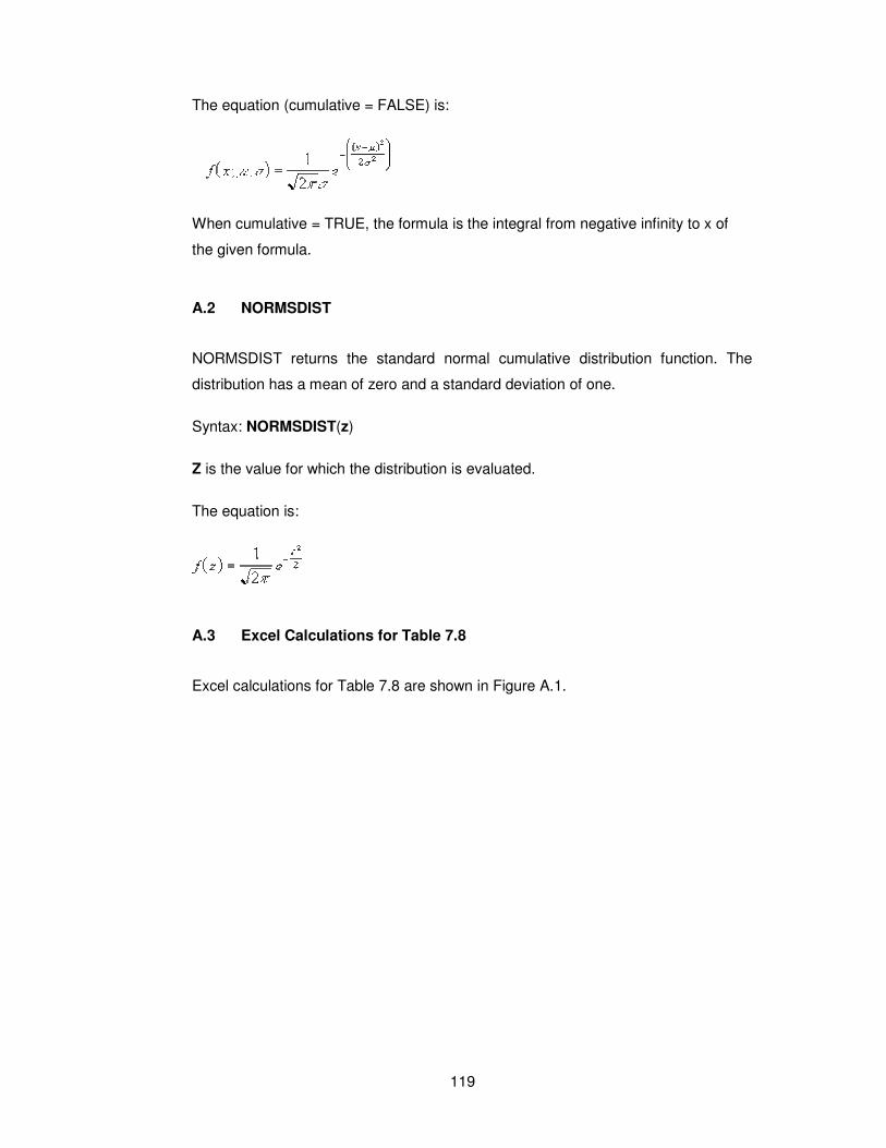
119

The equation (cumulative = FALSE) is:

When cumulative = TRUE, the formula is the integral from negative infinity to x of

the given formula.

A.2 NORMSDIST

NORMSDIST returns the standard normal cumulative distribution function. The

distribution has a mean of zero and a standard deviation of one.

Syntax: NORMSDIST(z)

Z is the value for which the distribution is evaluated.

The equation is:

A.3 Excel Calculations for Table 7.8

Excel calculations for Table 7.8 are shown in Figure A.1.

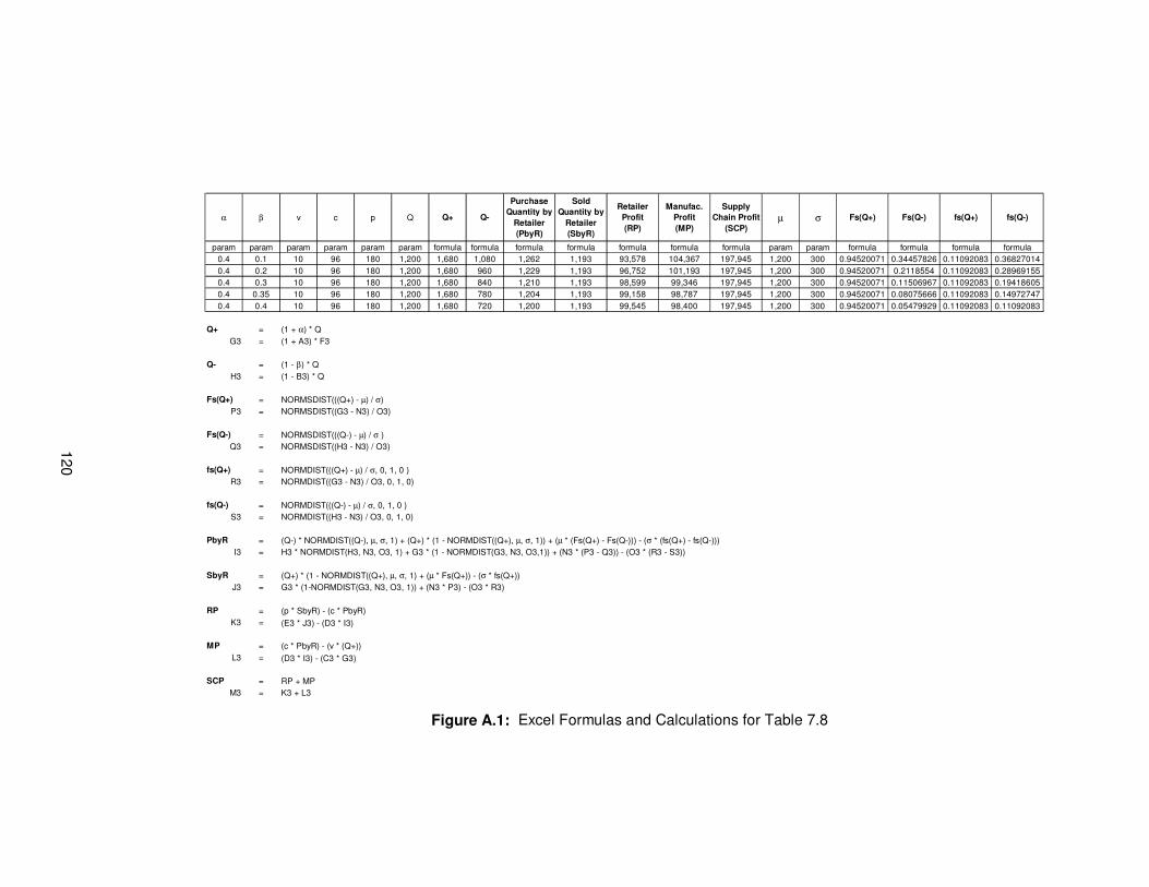
120

α β v c p Q Q+ Q-

Purchase Quantity by

Retailer (PbyR)

Sold Quantity by

Retailer (SbyR)

Retailer Profit (RP)

Manufac. Profit (MP)

Supply Chain Profit

(SCP)µ σ Fs(Q+) Fs(Q-) fs(Q+) fs(Q-)

param param param param param param formula formula formula formula formula formula formula param param formula formula formula formula0.4 0.1 10 96 180 1,200 1,680 1,080 1,262 1,193 93,578 104,367 197,945 1,200 300 0.94520071 0.34457826 0.11092083 0.368270140.4 0.2 10 96 180 1,200 1,680 960 1,229 1,193 96,752 101,193 197,945 1,200 300 0.94520071 0.2118554 0.11092083 0.289691550.4 0.3 10 96 180 1,200 1,680 840 1,210 1,193 98,599 99,346 197,945 1,200 300 0.94520071 0.11506967 0.11092083 0.194186050.4 0.35 10 96 180 1,200 1,680 780 1,204 1,193 99,158 98,787 197,945 1,200 300 0.94520071 0.08075666 0.11092083 0.149727470.4 0.4 10 96 180 1,200 1,680 720 1,200 1,193 99,545 98,400 197,945 1,200 300 0.94520071 0.05479929 0.11092083 0.11092083

Q+ = (1 + α) * QG3 = (1 + A3) * F3

Q- = (1 - β) * QH3 = (1 - B3) * Q

Fs(Q+) = NORMSDIST(((Q+) - µ) / σ)P3 = NORMSDIST((G3 - N3) / O3)

Fs(Q-) = NORMSDIST(((Q-) - µ) / σ )Q3 = NORMSDIST((H3 - N3) / O3)

fs(Q+) = NORMDIST(((Q+) - µ) / σ, 0, 1, 0 )R3 = NORMDIST((G3 - N3) / O3, 0, 1, 0)

fs(Q-) = NORMDIST(((Q-) - µ) / σ, 0, 1, 0 )S3 = NORMDIST((H3 - N3) / O3, 0, 1, 0)

PbyR = (Q-) * NORMDIST((Q-), µ, σ, 1) + (Q+) * (1 - NORMDIST((Q+), µ, σ, 1)) + (µ * (Fs(Q+) - Fs(Q-))) - (σ * (fs(Q+) - fs(Q-)))I3 = H3 * NORMDIST(H3, N3, O3, 1) + G3 * (1 - NORMDIST(G3, N3, O3,1)) + (N3 * (P3 - Q3)) - (O3 * (R3 - S3))

SbyR = (Q+) * (1 - NORMDIST((Q+), µ, σ, 1) + (µ * Fs(Q+)) - (σ * fs(Q+))J3 = G3 * (1-NORMDIST(G3, N3, O3, 1)) + (N3 * P3) - (O3 * R3)

RP = (p * SbyR) - (c * PbyR)K3 = (E3 * J3) - (D3 * I3)

MP = (c * PbyR) - (v * (Q+))L3 = (D3 * I3) - (C3 * G3)

SCP = RP + MPM3 = K3 + L3

Figure A.1: Excel Formulas and Calculations for Table 7.8

121

VITA

Murat ÖZMIZRAK was born October 29, 1951 in Ankara, Turkey. Murat has a

Master of Science in System Science degree from University of Ottawa and both

Master of Science and Bachelor of Science degrees in Industrial Engineering from

Boğaziçi University. After working as a software verification engineer for fifteen

years at Nortel Networks, he taught Web Development, Database Certification, and

Computer Engineering courses at Algonquin College, Ottawa. He is currently

working as an instructor at İstanbul Commerce University, teaching Industrial

Engineering and Computer Engineering courses. Murat is married and has a

wonderful daughter.