A Predictive Test of Voters’ Economic Benchmarking:The 2013 German Bundestag Election∗

Mark Andreas Kayser † Arndt Leininger ‡

21st November 2015

Abstract

Do voters judge their national economy relative to economic performance abroad?In 2013 we took advantage of the German Bundestag election to test this hypothesispredictively. Nearly two months prior to the election, we published an electionforecast relying on a theory-driven empirical model of election outcomes that drawson previous election outcomes; characteristics of the government and of voters; and,most originally, the relative economic performance of Germany (‘benchmarked”growth) in comparison to the three other most important economies in Europe,France, the UK and Italy. Our forecast put the outgoing coalition governmentof CDU/CSU and FDP at 47.05% of the popular vote deviating from the actualoutcome of 46.3 by 0.75 points. This makes our forecast one of the most accuratein this election cycle. Despite one and a half months of lead time, our forecastperformed on par or slightly better than the last poll results issued only two daysbefore the election.

∗Authors’ note: We gratefully acknowledge comments and suggestions by Michael Bolle, ThomasGschwend and Simon Munzert, as well as colloquium participants at the Jean Monet Centre, Free Uni-versity Berlin, conference participants at the ‘Gemeinsame Tagung der DVPW-Arbeitskreise ‘Politik undKommunikation’ und ‘Wahlen und politische Einstellungen’: Die Bundestagswahl 2013”, Wissenschaft-szentrum Berlin, and participants at the conference ‘Election Studies: Reviewing the Bundestagswahl2013”, Center for Advanced Studies, LMU Munich, organized by Andreas Graefe.†Hertie School of Governance, Berlin, e-mail: kayser@hertie-school.org‡Hertie School of Governance, Berlin, e-mail: a.leininger@phd.hertie-school.org

‘Forecasts are difficult – especially if they concern the future.’1

– Karl Valentin

1 Introduction

Predictive validity is a cornerstone of science, more difficult to achieve than explanation2

and correspondingly all too often neglected in the social sciences.3 In the run-up to the

German federal election of 2013, forecasts and prognostications about who would win

attracted considerable attention, both within Germany and beyond. We entered the fray,

using it as an opportunity to test a recent hypothesis about how voters form economic

evaluations about government performance.

The economy perennially serves as one of the most important determinants of electoral

outcomes4 but precisely how voters form their economic assessments is less clear. Re-

cently,5 claimed, and6 experimentally confirmed – in the case of Denmark and Sweden

– that voters judge national economic performance in comparison to that abroad. Such

effects emerge in observational data because the media report more positively on the

domestic economy when it outdistances its neighbors. Both the observational and ex-

perimental data of these respective studies, however, sought explanation rather than

prediction. Here we offer a different test, an election forecast estimated two months prior

to the 2013 Bundestag election based on a spartan model of voting behavior that in-

1‘Prognosen sind schwierig – vor allem, wenn sie die Zukunft betreffen” quote ascribed to Germancabaret artist Karl Valentin (1882-1948)

2Carl G Hempel. ‘Explanation and prediction by covering laws’. In: Philosophy of science: TheDelaware seminar. Vol. 1. New York: Wiley. 1963, pp. 107–33.

3Alexander Rosenberg. Economics–Mathematical Politics or Science of Diminishing Returns? Uni-versity of Chicago Press, 1992; Philip A Schrodt. ‘Seven deadly sins of contemporary quantitativepolitical analysis’. In: Journal of Peace Research 51.2 (2014), pp. 287–300; Milton Friedman. ‘Themethodology of positive economics’. In: Essays in positive economics 3.3 (1953).

4Richard Nadeau, Michael S Lewis-Beck and Eric Belanger. ‘Economics and elections revisited’. In:Comparative Political Studies 46.5 (2013), pp. 551–573.

5Mark Andreas Kayser and Michael Peress. ‘Benchmarking across Borders: Electoral Accountabilityand the Necessity of Comparison’. In: American Political Science Review 106.03 (Aug. 2012), pp. 661–684.

6Kasper M. Hansen, Asmus L. Olsen and Mickael Beck. ‘Cross-national Yardstick Comparisons: AChoice Experiment on a Forgotten Voter Heuristic’. In: Political Behavior (2013), p. xxx.

1

corporates only benchmarked (i.e., comparative) economic growth, previous vote share,

terms in office and partisan identification. To set our results in the context of what con-

stitutes an accurate prediction, we contrast our model’s performance with other forecasts

and polls,7 also ‘post-predicting” past elections out of sample and calculating average

prediction error.

There are many ways to forecast an election. Leaving casual punditry aside, prognostic-

ators can turn to structural models, survey polling – asking respondents whom they will

vote for or who they think will win – political betting markets, poll averaging techniques

and more recently, synthetic models8 that mix structural forecasts and polls. The 2013

Bundestag election saw a welcome expansion in the number of election forecasts in a

country that has historically had few.9 In contrast to many of the other forecasts, we

constructed a structural forecasting model that made no attempt at improving meth-

ods10; rather we employed simple linear regression with some of the most conventional

vote-choice predictors identified in electoral research. We added only a single innovation

intended to test whether voters use cross-national comparisons to assess the economy: in

place of economic growth, we employed the deviation in German real GDP growth from

that of its largest European benchmarks, the UK, France and Italy.

7As we address below, polls are snapshots in time (Will Jennings and Christopher Wlezien. ‘TheTimeline of Elections: A Comparative Perspective’. In: American Journal of Political Science [Forth-coming 2015]) rather than predictions of outcomes on election day. We account for this by evaluatingour forecast in comparison to polls taken shortly before (usually two days prior to) the election

8Robert S Erikson and Christopher Wlezien. ‘Forecasting US presidential elections using economicand noneconomic fundamentals’. In: PS: Political Science & Politics 47.02 (2014), pp. 313–316; MichaelS Lewis-Beck and Ruth Dassonneville. ‘Forecasting elections in Europe: Synthetic models’. In: Research& Politics 2.1 (2015), p. 2053168014565128.

9The notable exception are (Thomas Gschwend and Helmut Norpoth. ‘”Wenn am nachsten Sonntag...”: Ein Prognosemodell fur Bundestagswahlen’. In: Wahlen und Wahler: Analysen aus Anlass derBundestagswahl 1998. Ed. by Hans-Dieter Klingemann and Max Kaase. Wiesbaden: WestdeutscherVerlag, 2001, pp. 473–499) and (Bruno Jerome, Veronique Jerome-Speziari and Michael S. Lewis-Beck.A political-economy forecast for the 2009 German elections (September 27): The end of the GrandCoalition? 2009) whose Chancellor and Political Economy models were the only the only seriousforecasts for several elections.

10cf., for example, Peter Selb and Simon Munzert. Forecasting the 2013 Bundestag Election UsingData from Various Polls. SSRN Scholarly Paper ID 2313845. Rochester, NY: Social Science ResearchNetwork, Aug. 2013; Andreas Graefe et al. ‘Combining forecasts: An application to elections’. In:International Journal of Forecasting 30.1 (Jan. 2014), pp. 43–54; Bruno Jerome, Veronique Jerome-Speziari and Michael S. Lewis-Beck. ‘A Political-Economy Forecast for the 2013 German Elections:Who to Rule with Angela Merkel?’ In: PS: Political Science & Politics 46.03 (June 2013), pp. 479–480.

2

More specifically, our forecast, released in early August 2013,11 relies on a theory-driven

forecasting model of election outcomes that draws on previous election outcomes; char-

acteristics of the government and of voters; and, most originally, the relative economic

performance of Germany (‘benchmarked’ growth). It put the outgoing coalition govern-

ment of CDU/CSU and FDP at roughly 47.05% of the popular vote, 12 overshooting

the actual result by just .75 percentage points. This compares rather favorably to the

last poll results issued only two days before the election as well as to other forecast-

ing models. When we consider the average out-of-sample prediction error of the nine

most recent Bundestag elections – single forecasts can, of course, be misleading – our

benchmarking model also outperforms other models, including an identical model using

non-benchmarked growth.

Forecasting models have already made important theoretical contributions to electoral

research. Most notably, the volatility of political polls over a campaign contrasts sharply

with the ability of of fundamentals-based structural models to predict outcomes months

ahead of an election. This has highlighted the often ephemeral effects of events in elec-

tion campaigns and led to insights into when and how voters receive information and

form voting preferences.13 As elections near, they both pay more attention and weight

‘fundamentals” such as the economy more heavily.14 As15 points out, election forecasting

has contributed greatly to our understanding of the retrospective nature of the economic

vote. We hope that forecasts can similarly contribute to fundamental insights on the

effect of cross-national economic benchmarking on vote choice.

11FOCUS Online. Forscher sagen voraus: Union und FDP erreichen bei der Wahl exakt 47,05 Prozent.Aug. 2013.

12As originally reported in our early August forecast (ibid.).13Jennings and Wlezien, ‘The Timeline of Elections: A Comparative Perspective’.14Andrew Gelman and Gary King. ‘Why Are American Presidential Election Campaign Polls So

Variable When Votes Are So Predictable?’ In: British Journal of Political Science 23 (1993), pp. 409–451.

15William G. Mayer. ‘What, If Anything, Have We Learned from Presidential Election Forecasting?’en. In: PS: Political Science & Politics 47.02 (Apr. 2014), pp. 329–331.

3

2 Benchmarking and the Economic Vote

The effect of the economy on the vote is one of the most researched relationships in

the study of politics. Scholars, using a broad variety of objective economic variables as

well as surveys of perceived economic performance have assembled strong evidence across

national and institutional contexts demonstrating that voters punish the party in power

when the economy sours but reward it when the economy expands.16 Careful estimates

associate a unit change in economic growth with between a .8 and 1.4 percentage point

increase in the incumbent party’s vote share.17

Yet, for all of the scholarly confidence about the economic vote, considerable uncertainties

remain about how it arises and manifests itself.18 How do voters attribute responsibility

to specific governing parties?19 Do they punish governments more for downturns than

they reward them for expansions?20 How do institutions and political arrangements that

clarify or obfuscate party responsibility for outcomes influence attribution and voting?21

16Nadeau, Lewis-Beck and Belanger, ‘Economics and elections revisited’; Raymond M. Duch andRandy Stevenson. The Economic Vote: How Political and Economic Institutions Condition ElectionResults. Cambridge: Cambridge University Press, 2008.

17Michael Becher and Michael Donnelly. ‘Economic Performance, Individual Evaluations, and theVote: Investigating the Causal Mechanism’. In: The Journal of Politics 75.04 (Aug. 2013), pp. 968–979.

18Christopher J. Anderson. ‘The End of Economic Voting? Contingency Dilemmas and the Limits ofDemocratic Accountability’. In: Annual Review of Political Science 10.1 (2007), pp. 271–296; Mark A.Kayser. ‘The Elusive Economic Vote’. In: Comparing Democracies 4. Ed. by Lawrence LeDuc, RichardG. Niemi and Pippa Norris. Thousand Oaks, CA: Sage, 2014.

19David Fortunato and Randolph T Stevenson. ‘Performance Voting and Knowledge of Cabinet Com-position’. In: Electoral Studies 32 (2013), pp. 517–523; Raymond Duch and Randolph Stevenson. ‘Voterperceptions of agenda power and attribution of responsibility for economic performance’. In: ElectoralStudies 32 (2013), pp. 512–516.

20Stuart N. Soroka. ‘Good News and Bad News: Asymmetric Responses to Economic Information’. In:Journal of Politics 68.2 (May 2006), pp. 372–385; Piero Stanig. ‘Political Polarization in RetrospectiveEconomic Evaluations During Recessions and Recoveries ?’ In: Electoral Studies 32.4 (2013), pp. 729–745.

21Cameron D. Anderson. ‘Economic Voting and Multilevel Governance: A Comparative Individual-Level Analysis’. In: American Journal of Political Science 50.2 (Apr. 2006), pp. 449–463; TimothyHellwig. ‘Constructing Accountability’. In: Comparative Political Studies 45.1 (Jan. 2012), pp. 91–118;Sara Hobolt, James Tilley and Susan Banducci. ‘Clarity of responsibility: How government cohesionconditions performance voting’. In: European Journal of Political Research (2012); Bingham G. Powelland Guy D. Whitten. ‘A Cross-National Analysis of Economic Voting: Taking Account of the PoliticalContext’. In: American Journal of Political Science 37.2 (1993), pp. 391–414.

4

Do voters’ abilities22 and partisanship23 influence their response to economic change? Do

voters hold governing parties accountable for developments, economic and other, beyond

the government’s control?24

One fundamental issue is how voters evaluate the economy in the first place. A growth

rate of two percent would be welcomed as strong growth in much of Europe today but

looks anemic in the context of historic growth rates of earlier decades and would con-

stitute an economic crisis in contemporary China.25 addressed this issue eloquently with

respect to comparisons over time but it is only recently that scholars have considered

how the performance of foreign economies affects voters assessment of their own. Cross-

jurisdiction benchmarking has been an established empirical regularity in the study of

economic policies, especially tax rates, at least since the seminal work on ‘yardstick com-

petition” by.26 Only recently, however, has it gained attention in empirical voting studies

when27 demonstrated that benchmarked growth – the deviation in the growth rate from

that of comparison countries – predicts the vote for lead governing parties more strongly

than non-decomposed growth.

28 had already argued that voters are sufficiently informed to compare the variance in eco-

nomic outcomes across countries when assessing governmental performance and, indeed,29

22Brad T. Gomez and J. Matthew Wilson. ‘Cognitive Heterogeneity and Economic Voting: A Com-parative Analysis of Four Democratic Electorates’. In: American Journal of Political Science 50.1 (Jan.2006), pp. 127–145.

23Mark Andreas Kayser and Christopher Wlezien. ‘Performance pressure: Patterns of partisanshipand the economic vote’. In: European Journal of Political Research 50.3 (May 2011), pp. 365–394;Andrew Eggers. ‘Partisanship and Electoral Accountability : Evidence from the UK Expenses Scandal’.In: Quarterly Journal of Political Science (2015).

24Andrew J. Healy, Neil Malhotra and Cecilia H. Mo. ‘Irrelevant events affect voters’ evaluationsof government performance’. In: Proceedings of the National Academy of Sciences 107.29 (July 2010),pp. 12804–12809; Timothy T. Hellwig. ‘Interdependence, Government Constraints, and Economic Vot-ing’. In: Journal of Politics 63.4 (2001), pp. 1141–62.

25Harvey D. Palmer and Guy D. Whitten. ‘The Electoral Impact of Unexpected Inflation and EconomicGrowth’. In: British Journal of Political Science 29.04 (1999), pp. 623–639.

26Timothy Besley and Anne Case. ‘Incumbent Behavior: Vote-Seeking, Tax-Setting, and YardstickCompetition’. In: The American Economic Review 85.1 (1995), pp. 25–45.

27Kayser and Peress, ‘Benchmarking across Borders’.28Ray Duch and Randy Stevenson. ‘The Global Economy, Competency and the Economic Vote’. In:

Journal of Politics 72 (2010), pp. 105–123.29Hansen, Olsen and Beck, ‘Cross-national Yardstick Comparisons: A Choice Experiment on a For-

5

have shown in an experimental setting that when voters are informed of a comparison

country’s performance, they use it as a benchmark for holding their own governing parties

accountable.,30 however, are more skeptical of voter information levels and show, using

data from the Times of London that the press reports more positively on the economy

when it outperforms that of other countries, raising the possibility of ‘pre-benchmarking’.

Voters need not know anything about the performance of other economies so long as me-

dia reports on the economy influence their vote. Using a dataset of 32 newspapers from

16 countries in six languages31 indeed show that the effect of economic growth (but not

of inflation or unemployment) on the vote is heavily mediated by media reporting.

Such results are encouraging but the social science are littered with false positives32 and

the danger of confirmation bias33 lurks for scholars in all areas. Prediction offers an

alternative means to test for cross-national benchmarking in the economic vote and the

run-up to the 2013 Bundestag election offered promising conditions. The rate of real

GDP growth in Germany in the months prior to the election (.8% in the second and

.3% in the third quarter)34 was low compared to prior periods nevertheless higher than

the average of other large European economies still suffering from the aftermath of the

Financial Crisis, the Euro Crisis and/or fiscal austerity. If German voters judged the

economy only in absolute terms or in comparison to past growth, one would expect cross-

nationally benchmarked growth to emerge as a significantly weaker predictor than simple

real GDP growth and the forecasting model to predict the outcomes poorly. If they

indeed respond to relative growth, then benchmarked growth should predict the vote

more strongly than non-benchmarked growth and the model should predict the election

gotten Voter Heuristic’.30Kayser and Peress, ‘Benchmarking across Borders’.31Mark Andreas Kayser and Michael Peress. ‘The Media Mediates: How Voters Learn about the

Economy’. In: Working Paper (2015).32Stephan Choudoin, Jude Hays and Raymond Hicks. ‘Do we really know that the WTO cures

cancer? False positives and the effects of international institutions’. In: Paper presented at the 8thannual conference on the Political Economy of International Institutions, Berlin (2015).

33Raymond S Nickerson. ‘Confirmation bias: A ubiquitous phenomenon in many guises.’ In: Reviewof general psychology 2.2 (1998), p. 175.

34Federal Statistical Office. Seasonally adjusted quarterly results using Census X-12-ARIMA andBV4.1. 2015.

6

accurately. Of course, what constitutes accurate prediction must itself be benchmarked

against other predictions. We therefore survey other forecasting models next.

3 Other forecasting models

Electoral forecasting of the sort presented here, just like polling, originated in the context

of US presidential elections. While a small cottage industry has developed a variety of

models that perform rather well in the United States (see, for example, the 13 forecasts

in the October 2012 issue of PS: Political Science and Politics) election forecasting in

Germany is still in its infancy. Nevertheless, it is striking that to the best of our knowledge

our ‘benchmarking’ model was only the third model to be proposed for forecasting the

2013 German federal election – the others being the ‘Chancellor model’ first proposed

by35 who also provide a prediction for the upcoming election36 and a ‘Political Economy

Model’ by.3738 released a fourth forecast a bit later than ours.

Election forecasting in Germany was pioneered by.3940 Their forecasts provide a three-

months lead and they have a very good track record predicting the 2002, 2005 and

2009 elections. In 2002 they forecast the outgoing red-green government vote share

exactly right. Their model includes chancellor support (percentage of people favoring

the chancellor over his or her challenger), long-term partisanship (average of past three

election results of coalition parties) and the log of the number of terms the chancellor’s

party has been in government. Estimating their model over all past 16 elections and

35Gschwend and Norpoth, ‘”Wenn am nachsten Sonntag ...”: Ein Prognosemodell fur Bundestagswah-len’.

36Helmut Norpoth and Thomas Gschwend. ‘Chancellor Model Picks Merkel in 2013 German Election’.In: PS: Political Science & Politics 46.03 (June 2013), pp. 481–482.

37Jerome, Jerome-Speziari and Lewis-Beck, ‘A Political-Economy Forecast for the 2013 German Elec-tions’.

38Selb and Munzert, Forecasting the 2013 Bundestag Election Using Data from Various Polls.39Gschwend and Norpoth, ‘”Wenn am nachsten Sonntag ...”: Ein Prognosemodell fur Bundestagswah-

len’.40(Jerome, Jerome-Speziari and Lewis-Beck, A political-economy forecast for the 2009 German elections

(September 27): The end of the Grand Coalition? ) have also developed a forecasting model for Germanelections that they have used to forecast elections since 1998. They have published their forecasts in theFrench press and have received little attention in Germany.

7

fitting it to up-to-date data they provided not one but three slightly differing forecasts

for the 2013 election. These forecasts were, in chronological order, 51.7% vote share for

the outgoing government, published in July (but with data from April) in PS: Political

Science and Politics,41 49.7%, published on 26 July 2013 in a blog by the German weekly

Die Zeit,42 and 51.2% in another blog post on 24 August 2013.43 All forecasts were

produced using the same model, forecasts differ slightly because each time they use

updated polling data on chancellor approval. Technically, their model is similar to ours

but also their forecast is the farthest off of all models we review. They attribute this to

the unforeseen success of the Alternative fur Deutschland, a eurosceptic party founded

just months before the election, and the exceptional popularity of chancellor Merkel,

which extends well beyond her own party, diminishing the predictive quality of chancellor

support.44

45 have produced many forecasts of different national elections. For 2013 they presented

a new ‘Political Economy Model.’ They use a seemingly unrelated regression (SUR)

model to estimate the vote shares of all parties represented in parliament. Their variable

choice is also informed by electoral research and includes an economic measure like un-

employment but also political variables like chancellor approval as well as vote intention

polls. Their forecast of the coalition’s vote share is on par with ours but their estimates

for the opposition are slightly off. Their economic predictors are measured one to two

quarters before the election whereas some of their other political predictors are in prin-

ciple measurable even farther in advance, for instance whether the FDP was an outgoing

party with the CDU. They calculated their forecast in April 2013 using vote intention

41Norpoth and Gschwend, ‘Chancellor Model Picks Merkel in 2013 German Election’.42Zeit Blog. ‘Zweitstimme: Kanzlermodell sagt Wiederwahl von Merkel voraus’. In:

http://blog.zeit.de/zweitstimme/2013/07/26/kanzlermodell-sagt-wiederwahl-von-merkel-voraus/ (July2013).

43Zeit Blog. ‘Zweitstimme: Mach’s noch einmal, Mutti’. In:http://blog.zeit.de/zweitstimme/2013/08/24/machs-noch-einmal-mutti/ (Aug. 2013).

44Helmut Norpoth and Thomas Gschwend. ‘A Near Miss for the Chancellor Model’. In: EUSA: EUPolitical Economy Bulletin 17 (2014), pp. 4–8.

45Jerome, Jerome-Speziari and Lewis-Beck, ‘A Political-Economy Forecast for the 2013 German Elec-tions’.

8

polls available at the time (used to forecast vote shares of the Green Party, Die Linke

and the combined vote share of all other parties) which gives their model a lead of about

five months.

Selb and Munzert’s46 approach is similar to the above mentioned ones in using data from

prior elections to arrive at a forecast well ahead of the election. They differ in that

they exclusively rely on polling data. However by estimating the relationship between

pre-election polling and actual results they hope to eliminate the biases inherent in pre-

election polling which might be party- or polling-company specific and therefore arrive

at a more accurate forecast than the polls they use. Interestingly they find, based on

out-of-sample predictions, that they obtain the most accurate forecasts with polls taken

six months before the election. Accuracy decreases when using polls taken closer to the

election.

3.1 Polling

Polls differ markedly in technique and theory from forecasts; in fact they are atheoretical

and ahistorical. What they provide is a snapshot in time, not more and not less. Thus,

a poll, say, two months prior to an election, is not technically a forecast of the election,

although the media and voters often treat it as such.47 ‘Election-eve’ polls, however, are

much closer to predictions and, consequently, serve as a reasonable comparison for the

accuracy of our forecast.

Polling companies this year provided surprisingly accurate forecasts and substantially im-

proved their performance compared to previous elections. Forschungsgruppe Wahlen for

instance, the non-profit company behind the ZDF’s ‘Politbarometer’, provided estimates

of the coalition vote share that hovered between 45 and 47 percent since May 2013 (see

Figure 4). 2013 was an exceptionally good year for polling in Germany; in prior years even

46Selb and Munzert, Forecasting the 2013 Bundestag Election Using Data from Various Polls.47D. Sunshine Hillygus. ‘The Evolution of Election Polling in the United States’. en. In: Public

Opinion Quarterly 75.5 (Dec. 2011), pp. 962–981.

9

final pre-election polls have deviated considerably from the actual result.48 recently evalu-

ated 232 pre-election polls from 1957 to 2013 and found that conventional 95% confidence

intervals only contained the actual election result 69% of the time. In the prior election

in 2009, for instance, when the outgoing government was a grand coalition between the

CDU/CSU and the SPD the final pre-election ‘Politbarometer’ overestimated both the

vote share of the CDU/CSU and the SPD leading to an error of 4.2 percentage points.

This occurred partly because they underestimated the extent of ‘vote lending’ from CDU

to FDP – CDU supporters giving their second vote (‘Zweitstimme’) to the FDP.49 They

made no such mistake this time providing reasonable estimates for both CDU/CSU and

FDP. This might be due to improved methodology, however, the reform of the appor-

tionment system which eliminates the so-called ‘Uberhangmandate’ and therewith any

electoral advantage of ticket splitting may have been more important in this regard. All

point predictions from polls suggested an FDP vote share of 5% or more, while the FDP,

in fact, fell just below the 5% hurdle. The actual result for the FDP, however, is within

the poll’s margin of error.

4 Our model

Election forecasting in multi-party systems with proportional representation entails unique

challenges, these include multiple parties, coalition governments and strategic and mech-

anic effects of electoral thresholds. Most people are interested in forecasts because they

want to know who will win the election. However, in a multi-party system like Germany’s

the identity of the winner also depends on the outcome of post-election coalition bargain-

ing. Since it is difficult to predict winners or losers, it makes sense to focus rather on

parties’ vote shares, a determinant of the set of feasible governing coalitions. Specifically,

48Rainer Schnell and Marcel Noack. ‘The Accuracy of Pre-Election Polling of German General Elec-tions’. In: methods, data, analyses 8.1 (2014), pp. 5–24.

49These might be better described as ‘rental votes’ (Michael F. Meffert and Thomas Gschwend. ‘Stra-tegic coalition voting: Evidence from Austria’. In: Electoral Studies. Special Symposium: Voters andCoalition Governments 29.3 [Sept. 2010], pp. 339–349).

10

we focus on the vote share (to be) obtained by the outgoing governing coalition. The

coalition vote share is the percentage of the popular vote received by the parties forming

the governing coalition. This is usually the sum of the vote shares of two or more parties

– only once (in 1961) has Germany seen an outgoing single party government and even

then only when one counts the CDU and CSU as one party. We focus on the coalition’s

vote share, rather than on that of individual parties, because it is of the greatest sub-

stantive interest. With this forecast, we are able to predict whether the same government

will continue in power.

We thus make the assumption that a governing coalition wants to and will stay in power

if it secures the necessary votes to re-capture a parliamentary majority. Grand coalitions

are the exception here. They are mere coalitions of necessity (‘Staatsrason’) when no

other options involving a larger and one or more smaller parties seem feasible. Usually

neither coalition partner has an interest in continuing the coalition beyond the next

election. Furthermore, voters have no credible alternative government in opposition.

Our modeling choice – to use only the larger party’s vote share – was therefore motivated

by theory. The larger party in both of Germany’s grand coalitions (1969 and 2009) was

the CDU/CSU. For reasons we discuss further below our time-series is limited to 1980-

2013 and therefore only includes the latter. When faced with a coalition government,

voters attribute responsibility primary to the party of the prime minister,50 which in

Germany has always been is the larger coalition partner. Norpoth and Gschwend in their

forecasting model also rely on the larger party’s vote share for the same reasons.

Common predictors of a government’s electoral fortune work well for a time-series com-

posed of ‘regular’ coalitions and the larger party of a grand coalition but not if the full

vote share of a grand coalition is used. An alternative would be to use the grand coalition

vote share but include a grand coalition dummy variable. However, as our time-series

only contains one grand coalition, the dummy simply captures the difference in expec-

50Duch and Stevenson, The Economic Vote: How Political and Economic Institutions Condition Elec-tion Results; Duch and Stevenson, ‘Voter perceptions of agenda power and attribution of responsibilityfor economic performance’.

11

ted outcomes between grand-coalition and regular governments. In effect removing the

grand coalition from our time-series seems rather arbitrary to us. It also generates a

fundamental problem for forecasting models. If we were to forecast an election result

given an outgoing grand coalition – which is in fact what the situation will be in 2017

– our estimate would also be based on a model containing a coefficient that is based on

solely the deviation of one single election.

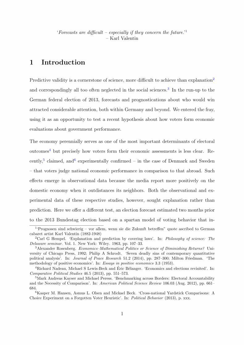
Figure 1: Predictors of the vote

19801983

19871990

1994

1998

2002

2005

2009

r = 0.9

3040

5060

35 40 45 50 55

Vote share in previous election

19801983

19871990

1994

1998

2002

2005

2009r = 0.6

3040

5060

25 30 35 40 45

Party Identification

198019831987 1990

1994

1998

2002

2005

2009r = 0.4

3040

5060

-2 0 2 4

Benchmarked growth

19801983

1987 1990

1994

1998

2002

2005

2009r = 0.1

3040

5060

0 .2 .4 .6 .8

Terms in office (logged)

Vot

e sh

are

obta

ined

by

outg

oing

gov

ernm

ent

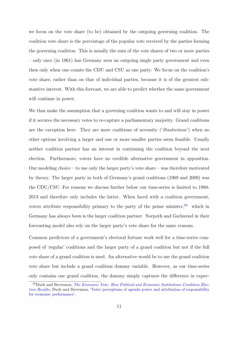
Four explanatory variables appear in our model: (1) the vote share received by the current

governing parties in the previous election, (2) the proportion of people identifying with

one of the governing parties, (3) the difference between Germany’s growth rate and the

‘benchmark’, i.e., the average of the growth rates in France, the UK and Italy, and (4)

the (log of the) number of terms a government has been in power. See Figure 1 for plots

of our dependent variable against our predictors. With the exception of the economic

benchmarking variable, an innovation for an election forecasting model, we chose these

variables for their broad acceptance as predictors of the vote in the voting literature.

12

We include the vote share of the current incumbent parties in the previous election (even

if they were not in government then) to form a baseline prediction. Past outcomes are

a strong predictor of future outcomes, so controlling for previous vote share effectively

focuses the other predictors on changes from the previous vote share. The combined vote

share of the parties making up the outgoing government correlates strongly with their

results in the previous election (r = 0.88). This is also because many people exhibit

strong partisanship, leading them to vote for the same party in successive elections.

Our second variable, party identification, captures the proportion of respondents express-

ing an attachment with one of the governing parties. Our data come from the Politbaro-

meter.51 The question put to respondents reads (our own translation), ‘Many people in

Germany lean toward a certain party, although they might vote for a different party from

time to time. What about you? Do you – generally speaking – lean toward a certain

party?’52 Party identification does not imply a formal attachment but, rather, simply

feeling close to a party. However, since the number of people with a party identification

still changes over the medium and long term, the proportion of people identifying with

one of the governing parties correlates significantly with the vote (r = 0.61). As party

identification has declined over the years, by about .6 percentage points per year,53 so has

the vote share obtained by the outgoing government. In the US setting, partisan identi-

fication is often the strongest predictor of vote choice.54 In Europe, scholars debate its

theoretical and empirical grounding in the context of multi-party systems but empirical

51We thank the Forschungsgruppe Wahlen for providing us with their 2013 aggregate party identific-ation data.

52‘In Deutschland neigen viele Leute langere Zeit einer bestimmten politischen Partei zu, obwohl sieauch ab und zu eine andere Partei wahlen. Wie ist das bei Ihnen: Neigen Sie – ganz allgemein gesprochen– einer bestimmten Partei zu?’ If respondants answer in the affirmative they are asked for the partythey lean toward and the strength of that orientation toward the named party. We use two of the threequestions used to measure party identification in the Politbarometer survey. We do not use the thirdquestion asking about the intensity of a citizen’s affinity to the party, that is we do not weigh respondentsby their answers to this question.

53Kai Arzheimer. ‘Mikrodeterminanten des Wahlverhaltens: Parteiidentifikation’. In: Wahlerverhal-ten in der Demokratie. Eine Einfuhrung. Ed. by Oscar W. Gabriel and Bettina Westle. StudienkursPolitikwissenschaft. Baden-Baden: Nomos, 2012, pp. 223–246.

54Angus Campbell et al. The American voter: Unabridged Edition. English. Chicago: The Universityof Chicago Press, 1960.

13

tests have demonstrated its stability in individuals over time and its sound performance

as a predictor in voting models.55 As party identification aggregates vary from month

to month by about 3%-points due to sampling error and idiosyncratic events56 we take

the average partisan identification for the governing parties in the six months before

the given election – for an election in September this would be the months of February

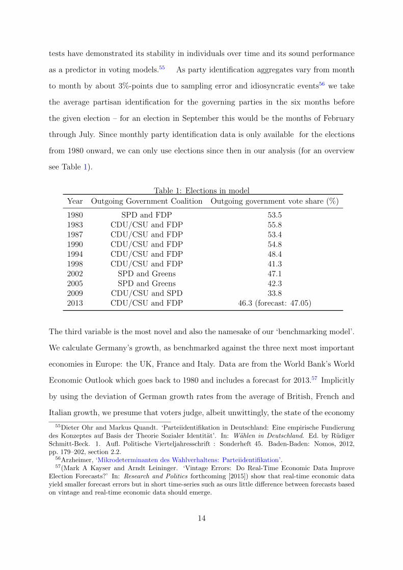
through July. Since monthly party identification data is only available for the elections

from 1980 onward, we can only use elections since then in our analysis (for an overview

see Table 1).

Table 1: Elections in model

Year Outgoing Government Coalition Outgoing government vote share (%)

1980 SPD and FDP 53.51983 CDU/CSU and FDP 55.81987 CDU/CSU and FDP 53.41990 CDU/CSU and FDP 54.81994 CDU/CSU and FDP 48.41998 CDU/CSU and FDP 41.32002 SPD and Greens 47.12005 SPD and Greens 42.32009 CDU/CSU and SPD 33.82013 CDU/CSU and FDP 46.3 (forecast: 47.05)

The third variable is the most novel and also the namesake of our ‘benchmarking model’.

We calculate Germany’s growth, as benchmarked against the three next most important

economies in Europe: the UK, France and Italy. Data are from the World Bank’s World

Economic Outlook which goes back to 1980 and includes a forecast for 2013.57 Implicitly

by using the deviation of German growth rates from the average of British, French and

Italian growth, we presume that voters judge, albeit unwittingly, the state of the economy

55Dieter Ohr and Markus Quandt. ‘Parteiidentifikation in Deutschland: Eine empirische Fundierungdes Konzeptes auf Basis der Theorie Sozialer Identitat’. In: Wahlen in Deutschland. Ed. by RudigerSchmitt-Beck. 1. Aufl. Politische Vierteljahresschrift : Sonderheft 45. Baden-Baden: Nomos, 2012,pp. 179–202, section 2.2.

56Arzheimer, ‘Mikrodeterminanten des Wahlverhaltens: Parteiidentifikation’.57(Mark A Kayser and Arndt Leininger. ‘Vintage Errors: Do Real-Time Economic Data Improve

Election Forecasts?’ In: Research and Politics forthcoming [2015]) show that real-time economic datayield smaller forecast errors but in short time-series such as ours little difference between forecasts basedon vintage and real-time economic data should emerge.

14

relative to that of other countries. Evidence of such ‘benchmarking across borders’ comes

from58 who explain the phenomenon with evidence that the media report more positively

on the economy when it is outperforming that of comparison countries. This measure

of relative economic performance is of special importance to the forecast for the 2013

election since German growth is sluggish but looks better when compared to that of

other European states suffering from the aftermath of the financial and Euro crises.

Indeed, of the 16 national governments up for re-election within an 18 months period

from July 2008 to the end of 2009 only nine of them lost vote share.59 Yet, their economic

performance was similarly dismal to that experienced by the OECD in general, with every

country experiencing at least two quarters of negative growth in this period and 13 of 16

experiencing negative growth in the quarter of or before the election.

Lastly, we rely on the empirical regularity that governments, on average, lose support

the longer they remain in office.60 The major governing parties (CDU/CSU or SPD) in

Germany have on average lost 3.2 percentage points per term. We capture this with the

log10 of the number of terms that a government has been in office.

4.1 Model estimates

Putting all variables in one linear regression model estimated over the elections 1980-2009

we can explain 99% of the variance in the vote share of the outgoing government in the

past 9 elections (see Table 2). An R2 of this magnitude raises worries about possibly

fitting noise but we were hesitant to change our specification due to too good a fit. All

coefficients are statistically significant and have the expected sign. Our first predictor

58Kayser and Peress, ‘Benchmarking across Borders’.59The sample is defined as all countries that held a general election or, in the case of the United States a

presidential election, between July 2008 and December 2008, which was recorded in the election appendixof the European Journal of Political Research.They are Austria, Bulgaria, Canada, Germany, Greece,Iceland, Israel, Japan, Luxembourg, Lithuania, New Zealand, Norway, Portugal, Romania, Slovenia, andthe United States.

60Martin Paldam. ‘The distribution of election results and the two explanations of the cost of ruling’.In: European Journal of Political Economy 2.1 (1986), pp. 5–24; Jane Green and Will Jennings. ThePolitics of Competence: The Nature and Implications of Public Opinion about Party Competence. BookManuscript. in progress. Chap. 5, Ch.5.

15

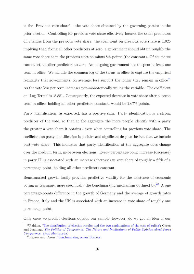
is the ‘Previous vote share’ – the vote share obtained by the governing parties in the

prior election. Controlling for previous vote share effectively focuses the other predictors

on changes from the previous vote share: the coefficient on previous vote share is 1.025

implying that, fixing all other predictors at zero, a government should obtain roughly the

same vote share as in the previous election minus 8%-points (the constant). Of course we

cannot set all other predictors to zero. An outgoing government has to spent at least one

term in office. We include the common log of the terms in office to capture the empirical

regularity that governments, on average, lose support the longer they remain in office61

As the vote loss per term increases non-monotonically we log the variable. The coefficient

on ‘Log Terms’ is -8.881. Consequently, the expected decrease in vote share after a secon

term in office, holding all other predictors constant, would be 2.67%-points.

Party identification, as expected, has a positive sign. Party identification is a strong

predictor of the vote, so that at the aggregate the more people identify with a party

the greater a vote share it obtains - even when controlling for previous vote share. The

coefficient on party identification is positive and significant despite the fact that we include

past vote share. This indicates that party identification at the aggregate does change

over the medium term, in-between elections. Every percentage-point increase (decrease)

in party ID is associated with an increase (decrease) in vote share of roughly a fifth of a

percentage point, holding all other predictors constant.

Benchmarked growth lastly provides predictive validity for the existence of economic

voting in Germany, more specifically the benchmarking mechanism outlined by.62 A one

percentage-points difference in the growth of Germany and the average of growth rates

in France, Italy and the UK is associated with an increase in vote share of roughly one

percentage-point.

Only once we predict elections outside our sample, however, do we get an idea of our

61Paldam, ‘The distribution of election results and the two explanations of the cost of ruling’; Greenand Jennings, The Politics of Competence: The Nature and Implications of Public Opinion about PartyCompetence. Book Manuscript.

62Kayser and Peress, ‘Benchmarking across Borders’.

16

Table 2: A regression model of past elections to predict future elections

Predictors Coefficient (S.E.)

Previous Vote Share 1.025*** (0.0544)Party ID 0.276** (0.0563)Benchmarked Growth 0.930* (0.224)Log Terms -8.881** (1.295)Constant -8.708* (2.724)

Observations 9R-squared 0.993Adj. R2 0.986RMSE∗ 1.424Durbin-Watson d 2.561

Standard errors in parentheses*** p<0.001, ** p<0.01, * p<0.05

∗ RMSE calculated from 9 out-of-sample predictions for elections 1980 to 2009.Note: Model estimated on elections 1980-2009

model’s predictive validity. The 2013 election provided an essential test in that regard.

In hindsight we know that it fared quite well, but when we constructed our model in

early summer 2013 we had to rely on other means to test our model’s ability to make

out-of-sample predictions. We did so with the help of out-of-sample predictions. By

omitting one election, re-estimating the model on the remaining elections and calculating

a prediction using the values of the omitted observation we ‘post-predicted’ historical

elections to test our model.63 We did this for all 9 previous elections, compared our

prediction to the actual outcome, squared the differences, averaged them and, finally,

took the square root to obtain the root mean square error (RMSE).

The RMSE gives us an estimate of the ‘average’ error of our model in out-of-sample

forecasting. Figure 3 plots the actual vote shares received by the outgoing government

against our prediction. The farthest we are off is 1.8 percentage points in 2005; in

63Due to the size of our dataset (n=9) we were not able to rely on consecutive out-of-sample forecastspredicting one observation ahead. Instead, we predicted the omitted election using also elections followingthe election to be predicted. Consequently, only our 2009 forecast is a true out-of-sample forecast intothe future. All other out-of-sample forecast predict a value within or at the beginning of the time-seriesused to fit the model.

17

1983 we get within one tenth of a percentage point of the actual result. The RMSE

for our model is 1.4 percentage points which, considering that the model only rests on

nine previous elections, compares rather favorably to standard errors of the regression

in surveys involving many more observations. Our coefficients remain stable across all

out-of-sample estimations showing that our results are not unduly influenced by outliers

and that the effects of our explanatory variables are, as we expected, stable over time

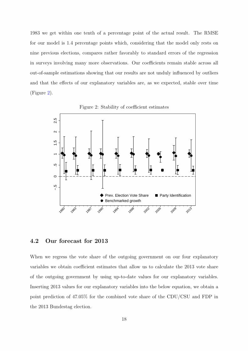
(Figure 2).

Figure 2: Stability of coefficient estimates

−.5

0.5

11.

52

2.5

1980

1983

1987

1990

1994

1998

2002

2005

2009

2013

Prev. Election Vote Share Party IdentificationBenchmarked growth

4.2 Our forecast for 2013

When we regress the vote share of the outgoing government on our four explanatory

variables we obtain coefficient estimates that allow us to calculate the 2013 vote share

of the outgoing government by using up-to-date values for our explanatory variables.

Inserting 2013 values for our explanatory variables into the below equation, we obtain a

point prediction of 47.05% for the combined vote share of the CDU/CSU and FDP in

the 2013 Bundestag election.

18

Outgoing government vote share = −8.708 + 1.025 ∗ vote share in previous election+

0.276 ∗ party identification + 0.930 ∗ benchmarked growth− 8.881(log10(terms))

Using the RMSE calculated from our ‘out-of-sample’ predictions we can calculate the

probability of the coalition obtaining a majority of seats in parliament necessary to con-

tinue in office. As this year’s change to the electoral system in Germany largely eliminates

distortions of the vote-seat relationship arising from so called ‘Uberhangmandate’ we only

have to worry about the votes obtained by parties that will not be represented in parlia-

ment. Polling prior to the election suggested that about 8%64 to 9.5%65 of votes would

go to the Pirates, Alternative fur Deutschland and other fringe parties that would likely

not exceed the 5% threshold. We assumed that the FDP and Die Linke would clear the

threshold. Die Linke was consistently well above 5-percent while the FDP would, so we

thought, again profit from ‘rental votes’ from CDU/CSU-voters which polls have diffi-

culty predicting. Of course, as we now know, the FDP stumbled on the 5% threshold.

We discuss this issue below.

Considering the substantial error in poll-based projections 2 months ahead of the elections

this gave us a range of 6 to 12 percentage points. If the polling for these minor parties was

correct, however, about 45.5% of the vote should suffice for Mrs. Merkel to continue the

coalition of CDU/CSU and FDP. Our point prediction already was above this threshold;

taking into account the statistical error inherent in the forecast, we predicted a 83%

probability that the outgoing coalition would have a majority in the next parliament.

In hindsight, the complex assumptions necessary to estimate this probability and the

fact that the FDP did not, in fact, obtain the minimal 5% vote share necessary to enter

parliament, may make our probability estimate seem overly naive as we discuss in section

6. However, the presentation of the election prediction as a probability is a useful exercise

64Forschungsgruppe Wahlen 24.07.2013, Infratest Dimap 25.07.201365Allensbach 12.07.2013

19

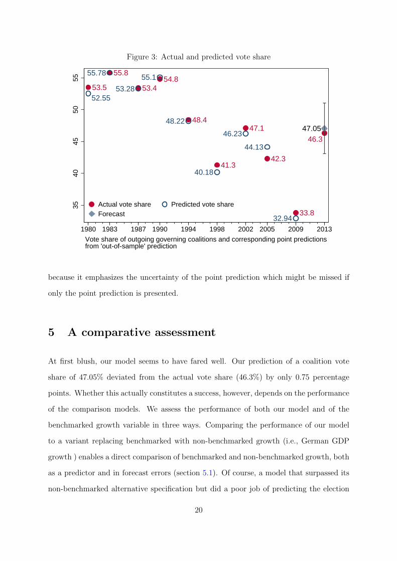
Figure 3: Actual and predicted vote share

53.5

55.8

53.454.8

48.4

41.3

47.1

42.3

33.8

46.3

52.55

55.78

53.28

55.1

48.22

40.18

46.23

44.13

32.94

47.05

3540

4550

55

1980 1983 1987 1990 1994 1998 2002 2005 2009 2013

Actual vote share Predicted vote shareForecast

Vote share of outgoing governing coalitions and corresponding point predictionsfrom 'out-of-sample' prediction

because it emphasizes the uncertainty of the point prediction which might be missed if

only the point prediction is presented.

5 A comparative assessment

At first blush, our model seems to have fared well. Our prediction of a coalition vote

share of 47.05% deviated from the actual vote share (46.3%) by only 0.75 percentage

points. Whether this actually constitutes a success, however, depends on the performance

of the comparison models. We assess the performance of both our model and of the

benchmarked growth variable in three ways. Comparing the performance of our model

to a variant replacing benchmarked with non-benchmarked growth (i.e., German GDP

growth ) enables a direct comparison of benchmarked and non-benchmarked growth, both

as a predictor and in forecast errors (section 5.1). Of course, a model that surpassed its

non-benchmarked alternative specification but did a poor job of predicting the election

20

would not necessarily be of much use. We therefore place our benchmarking model’s

performance in context by comparing it to other forecasts of the 2013 election and the

final election polls, two days before the election (section 5.2).

5.1 A forecast with non-benchmarked growth

To assess whether benchmarked growth is a superior predictor to real growth in GDP

– probably the most common economic measure in structural election forecasting mod-

els – we compare two forms of our model, one with benchmarked growth and one with

non-benchmarked growth in German real GDP. We are wary about over-drawing conclu-

sions based on the small sample size, the results are nevertheless informative, given the

constraints of the data.

benchmarked not benchmarked

Previous Vote Share 1.025∗∗∗ 0.789∗∗

(0.0544) (0.163)

Party ID 0.276∗∗ 0.395∗∗

(0.0563) (0.0834)

Benchmarked Growth 0.930∗

(0.224)

Growth Germany 0.693(0.426)

Log Terms -8.881∗∗ -9.616∗

(1.295) (2.618)

Constant -8.708∗ -1.335(2.724) (8.194)

MAE 1.01 2.09RMSE 1.42 2.472013 Forecast 47.05 45.79

N 9 9R2 0.993 0.978adj. R2 0.986 0.956

Table 3: A comparison of benchmarked and non-benchmarkedgrowth. Standard errors in parentheses. ∗ p < 0.05, ∗∗ p <0.01, ∗∗∗ p < 0.001

21

Benchmarked growth reveals a stronger effect than its non-benchmarked growth, as shown

in Table 5.1, associating a unit change with correspondingly larger increase (.93 v. .69) in

predicted vote share for the coalition. Benchmarked growth is also more precisely estim-

ated than its non-benchmarked counterpart. But how did the models fare in predicting

out-of-sample elections?

When all elections are predicted, one-by-one, out of sample, benchmarked growth outper-

forms its non-benchmarked alternative: When growth is benchmarked, the mean average

error (MAE) and root mean squared error (RMSE) of the model were 48% and 57% as

large, respectively, as when it was not. In other words, the forecast error from the model

with the non-benchmarked growth was over twice as large (2.09 v. 1.01) when measured

as MAE and 1.74 times as large measured as RMSE.

For the 2013 election, the point forecasts from both models deviated from from the

final outcome by less than a percentage point. While the forecast error from the non-

benchmarked model was even slightly smaller than that from the benchmarked model

they were not statistically distinguishable from each other at normal significance levels.

We further note that the non-benchmarked growth model predicts a smaller vote share

than the original model and actually underestimates the actual result. This suggests

that in contexts such as the 2013 German election, when Germany had sluggish growth

compared to prior periods but relatively high growth rates when compared to other

Eurozone economies, using non-benchmarked growth may underestimate the popularity

of the government.

In sum, while non-benchmarked growth actually produced a slightly more accurate pre-

diction for 2013, benchmarked growth produced more accurate out-of-sample predictions

in most of the other eight elections, yielding an average prediction error roughly half the

size of that from the non-benchmarked model.

22

5.2 Other forecasts and polls

Let us also benchmark our benchmarking model. It is informative to see how a simple

structural forecasting model with benchmarked growth performs relative to one with

non-benchmarked growth. But this comparison would be of less interest if both models

predicted poorly relative to other approaches. How did our benchmarking model fare

relative to other forecasts estimated well before the election and polls taken nearly on its

eve?

Our forecast put the outgoing coalition government of CDU/CSU and FDP at 47.05%

of the popular vote – quite close to the 46.3% it actually obtained.66 This makes our

forecast one of the most accurate among the forecasts that were released prior to the

election. Only one other forecast67 provided similar accuracy. Our forecast was also on

par or slightly more accurate than the last poll results collected only two days before the

election (for a quick comparison of forecasts, final polls and results see Table 4). It also

bested averages of pre-election polls, as well as average predictions of expert assessments

and prediction markets. These have been calculated by68 for his ‘PollyVote’ forecast. It

is produced through calculation of simple averages of the forecasts in four categories of

forecasts: polls, prediction markets, expert judgment and quantitative models. Graefe

also calculates the overall average across the categories.

He explicitly calculates simple averages because as he argues there are no advantages in

terms of accuracy in using more complicated averaging procedures. The idea behind aver-

aging over different forecasting methods is that no individual method that the PollyVote

model relies on is consistently better than the other. In fact, in an analysis of six elections

from 1992 to 201269 found that ‘methods that provided the most accurate forecasts in one

66Taking the additional step of assuming FDP inclusion in the next parliament and estimating thecoalition reelection probability appears, in retrospect, to have been less well advised.

67Jerome, Jerome-Speziari and Lewis-Beck, ‘A Political-Economy Forecast for the 2013 German Elec-tions’.

68Andreas Graefe. ‘German Election Forecasting: Comparing and Combining Methods for 2013’. In:German Politics forthcoming (2015).

69Graefe et al., ‘Combining forecasts’.

23

election were often among the least accurate in another election.’ For 2013 the PollyVote

aggregate was more accurate than any of the four component methods, however it was

not the single most accurate model. Thus, overall, our benchmarking model fared well

but we need to acknowledge that there is no guarantee that it will remain as accurate

in the future.

Table 4: Election result, forecasts and final pre-election polls

OfficialRes-ults

Kayser& Lein-inger

Norpoth&Gschwend

Jeromeet al

Selb &Munzert

Forschungs-gruppeWahlen,09/19

Forsa,09/20

Allensbach,09/20

Coalition 46.3 47.05(.75)

51.2(4.9)

47

(.7)

43.5(-2.8)

45.5(-.8)

45(-1.3)

45(-1.3)

CDU/CSU41.5 41(-.5)

38.1(3.4)

40(-1.5)

40(-1.5)

39.5(-2)

FDP 4.8 6(1.2)

5.4(.6)

5.5(-.7)

5(.2)

5.5(.7)

SPD 25.7 28(2.3)

28.2(2.5)

27(1.3)

26(.3)

27(1.3)

Bundnis90 / DieGrunen

8.4 10(1.6)

13.5(5.1)

9(.6)

10(1.6)

9(.6)

DieLinke

8.6 9(.4)

7.7(-.9)

8.5(.1)

9(.4)

9(.4)

Others 10.9 6(-4.9)

6.5(-.4.4)

10(-.9)

10(-.9)

10(-.9)

MAE - .75 4.9 1.82 2.82 .84 .89 .89

Numbers in parentheses indicate difference to official results.

5.3 Other assessment criteria

Accuracy, of course, is not the only criterion in assessing which forecast fared best.

Forecast assessment is multifaceted and many other criteria demand consideration.70

Parsimony, forecasting with a small number of predictors, is valuable where observations

70Michael S. Lewis-Beck. ‘Election forecasting: principles and practice’. In: The British Journal ofPolitics & International Relations 7.2 (2005), pp. 145–164.

24

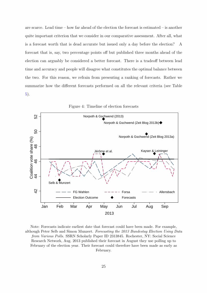
are scarce. Lead time – how far ahead of the election the forecast is estimated – is another

quite important criterion that we consider in our comparative assessment. After all, what

is a forecast worth that is dead accurate but issued only a day before the election? A

forecast that is, say, two percentage points off but published three months ahead of the

election can arguably be considered a better forecast. There is a tradeoff between lead

time and accuracy and people will disagree what constitutes the optimal balance between

the two. For this reason, we refrain from presenting a ranking of forecasts. Rather we

summarize how the different forecasts performed on all the relevant criteria (see Table

5).

Figure 4: Timeline of election forecasts

Kayser & Leininger

Norpoth & Gschwend (Zeit Blog 2013b)

Norpoth & Gschwend (Zeit Blog 2013a)

Norpoth & Gschwend (2013)

Jérôme et al.

Selb & Munzert

4244

4648

5052

Coa

litio

n vo

te s

hare

(%

)

Jan Feb Mar Apr May Jun Jul Aug Sep

2013

FG Wahlen Forsa Allensbach

Election Outcome Forecasts

Note: Forecasts indicate earliest date that forecast could have been made. For example,although Peter Selb and Simon Munzert. Forecasting the 2013 Bundestag Election Using Data

from Various Polls. SSRN Scholarly Paper ID 2313845. Rochester, NY: Social ScienceResearch Network, Aug. 2013 published their forecast in August they use polling up toFebruary of the election year. Their forecast could therefore have been made as early as

February.

25

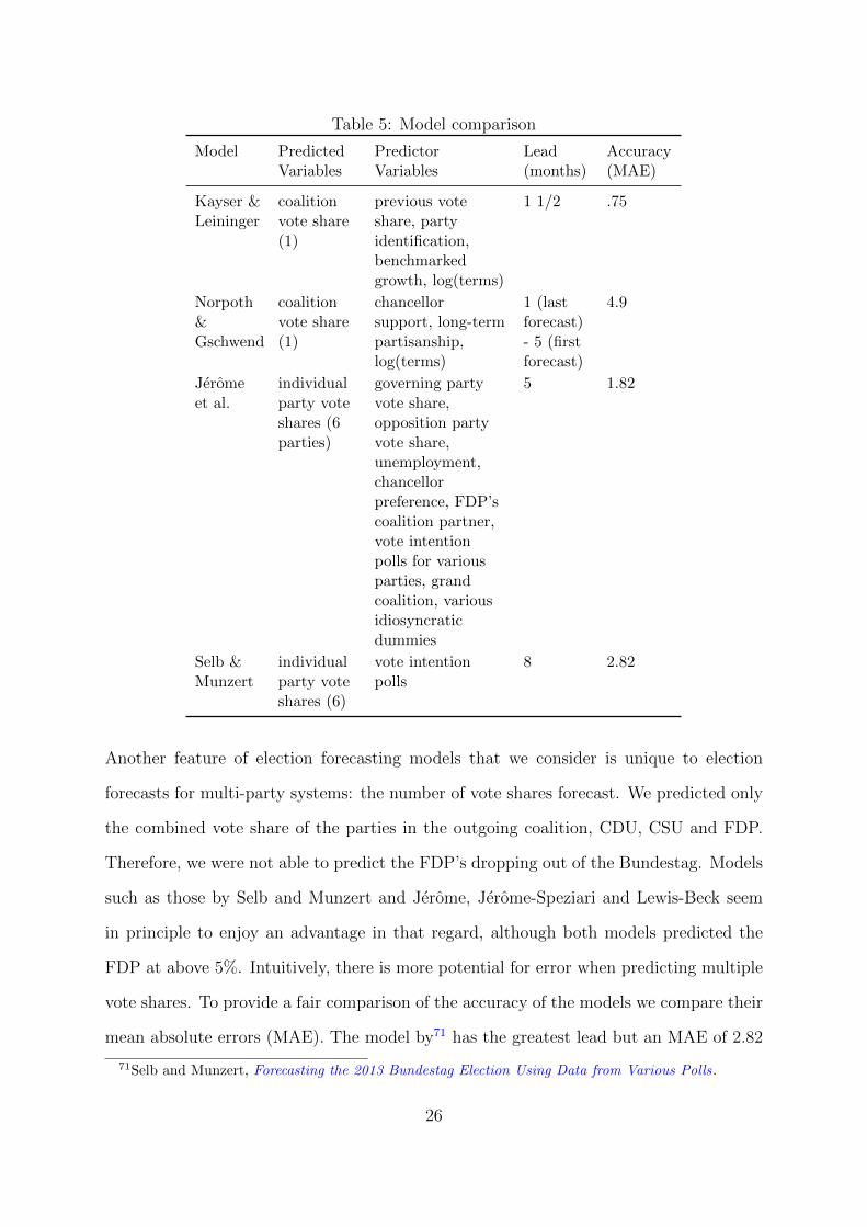
Table 5: Model comparison

Model PredictedVariables

PredictorVariables

Lead(months)

Accuracy(MAE)

Kayser &Leininger

coalitionvote share(1)

previous voteshare, partyidentification,benchmarkedgrowth, log(terms)

1 1/2 .75

Norpoth&Gschwend

coalitionvote share(1)

chancellorsupport, long-termpartisanship,log(terms)

1 (lastforecast)- 5 (firstforecast)

4.9

Jeromeet al.

individualparty voteshares (6parties)

governing partyvote share,opposition partyvote share,unemployment,chancellorpreference, FDP’scoalition partner,vote intentionpolls for variousparties, grandcoalition, variousidiosyncraticdummies

5 1.82

Selb &Munzert

individualparty voteshares (6)

vote intentionpolls

8 2.82

Another feature of election forecasting models that we consider is unique to election

forecasts for multi-party systems: the number of vote shares forecast. We predicted only

the combined vote share of the parties in the outgoing coalition, CDU, CSU and FDP.

Therefore, we were not able to predict the FDP’s dropping out of the Bundestag. Models

such as those by Selb and Munzert and Jerome, Jerome-Speziari and Lewis-Beck seem

in principle to enjoy an advantage in that regard, although both models predicted the

FDP at above 5%. Intuitively, there is more potential for error when predicting multiple

vote shares. To provide a fair comparison of the accuracy of the models we compare their

mean absolute errors (MAE). The model by71 has the greatest lead but an MAE of 2.82

71Selb and Munzert, Forecasting the 2013 Bundestag Election Using Data from Various Polls.

26

percentages points. Our model has the smallest MAE of .75 percentage points but we also

have the smallest lead of just one and a half months and we only predict coalition vote

share. Considering that the forecasts were made months ahead of the election we believe

all of the forecasting models compare quite well to the last pre-election polls issued only

days before the election. These were quite accurate but they have practically no lead

time (see Table 4).

One model can provide different forecasts, so can have multiple different lead times. For

instance Norpoth and Gschwend provided three forecasts in 2013 based on updated data

on their poll-based predictor variable chancellor popularity. The limiting factor in our

model is also a poll-based variable, party identification in our case. As we published our

forecast in early August we chose to incorporate the latest available data. We conducted

several out-of-sample forecasts, post-hoc varying the lead time, and found that the average

forecasting error tends to increase with lead time. For future elections we could provide

monthly updates to our forecast by changing the measure of party identification – by

adding the newest Politbarometer month to the average and dropping the last – with the

promise of increasing the accuracy of our forecast as the election draws nearer. Structural

models also provide the opportunity to calculate scenarios. Instead of waiting for new

data to come in one can use a range of likely values to calculate corresponding forecasts.

6 Discussion: Election Forecasting in Germany

The 2013 election exposed two problems with forecasting models that focus on coalition

vote share. First, estimating the probability of a government remaining in power is

considerably more difficult than providing a point estimate of its vote share. For the

former one has to identify a vote threshold that will likely guarantee a parliamentary

majority. We estimated this threshold to be 45.5% given the likely vote shares to be

obtained by parties not surpassing the 5% threshold. However to calculate this threshold

we ultimately had to rely on the polls that we aimed to outperform. Second, as we did

27

not forecast individual party vote shares, we again had to rely on polls to gauge the

likelihood of all coalition parties re-entering parliament. Based on our point prediction

we calculated a 83% probability that the outgoing coalition will have a majority in the

next parliament. We calculated that probability as a one-sided hypothesis test, treating

the effective threshold of 45.5% as null hypothesis. We naively put the FPD’s probability

of making the threshold at 1, which is obviously wrong as we now know. In hindsight

we believe we could have done better. Rather than taking the polls at face value we

should have, as one always should with polling data, accounted for the random error. We

should have calculated the probability of the FDP surpassing the threshold and included

that information in calculating the probability of the government continuing. Models

such as those provided by72 and73 have a clear advantage in that regard as they provide

predictions for all parties.

This election also posed a unique challenge to all election forecasters due to the change

in the apportionment system. A reform mandated by Germany’s constitutional court

eliminated the so-called Uberhangmandate, drastically reducing the incentive for stra-

tegic voting. Without the reform, forecasts would likely have been more accurate. The

reduction of split-ticket voting74 also goes towards explaining the increased accuracy of

pre-election polling.

Minor parties pose another challenge to election forecasters and not only in multi-party

systems – think of third party candidates in the US. They matter more, however, in

multi-party systems. Forecasts of US presidential elections usually predict the incumbent

party’s share of the two-party popular vote (rather than of the total vote) to account for

third party candidates taking some of the vote which in the end is politically inconsequen-

tial. Forecasters of German Bundestag elections could similarly forecast the in-Bundestag

72Jerome, Jerome-Speziari and Lewis-Beck, ‘A Political-Economy Forecast for the 2013 German Elec-tions’.

73Selb and Munzert, Forecasting the 2013 Bundestag Election Using Data from Various Polls.74Kathleen Bawn. ‘Voter Responses to Electoral Complexity: Ticket Splitting, Rational Voters and

Representation in the Federal Republic of Germany’. In: British Journal of Political Science 29.03(1999), pp. 487–505.

28

vote share, the incumbent coalition’s vote share relative to the vote share obtained by

all parties surpassing the 5%-threshold needed to be represented in the Bundestag. Such

forecasts would be hard to communicate to the public as coverage of the horse race fo-

cuses on overall vote share. Presenting such forecasts in seat shares – especially since the

reform of the electoral systems promises to make vote share more proportional to seat

share – might be more viable.

Another complication that also applies to election forecasts beyond Germany arises from

small sample size. For a good forecast we want the error around the prediction to be

as small as possible – it should be comparable to confidence intervals in survey research.

Given the low number of post-war elections, a forecasting model, besides having all

coefficients significant, needs a good fit. Most forecasting models haven an R2 well above

.9. However, also due to the low number of observations, one runs the risk of over-fitting

the model – fitting some of the random noise inherent in elections. Striking a balance

between tightly fitting and over-fitting the model is a challenge that seems to be as much

art as science.

These problems decrease only slightly with every additional Bundestag election held. Yet,

there are alternatives to waiting four years for the next election to expand one’s dataset

by one observation. Several authors estimate forecasting models at the district and state

level and aggregate the results up to arrive at a national prediction.7576 presents the first

attempt at constituency-level election forecasting for Germany. Such an approach has

certain advantages. In the US the winner of the popular vote might be the loser of the

Electoral College vote, which is precisely what happened to Al Gore in 2000. Furthermore,

not just national but also regional factors determine national election outcomes and

combining district or state time-series yields a much larger dataset allowing the estimation

75Carl E. Klarner. ‘State-Level Forecasts of the 2012 Federal and Gubernatorial Elections’. en.In: PS: Political Science & Politics 45.04 (Oct. 2012), pp. 655–662; Bruno Jerome and VeroniqueJerome-Speziari. ‘Forecasting the 2012 US Presidential Election: Lessons from a State-by-State PoliticalEconomy Model’. en. In: PS: Political Science & Politics 45.04 (Oct. 2012), pp. 663–668.

76Simon Munzert. ‘A Methodological Framework for Constituency-Level Election Forecasting’. In:Working Paper (2015).

29

of more complex models. These reasons in part also apply to the German context as voters

vote for regional not national party lists and seat shares are allocated at the regional

level. Disaggregating to a lower level also allows forecasters to account for regional

peculiarities, for instance the CSU in Bavaria or the strong performance of Die Linke in

Eastern Germany (or greater number of protest voters in Eastern Germany).

6.1 Election Forecasting: what is it good for?

Election forecast are not without criticism. Particularly structural models like ours which

are macro-level models of what in the end is an individual-level act – voting – are the

object of criticism. They are estimated from small samples and rely on the assumption

of time-invariant effects. Therefore, they seem destined to go wrong or require ad-hoc

fixes, that may seem arbitrary, if circumstances change..

Such has been the topic of a debate between77 and78 in a 2005 post-election issue of

Politische Vierteljahresschrift. Klein criticizes Norpoth and Gschwend for a one-time

correction to their model, adjusting one variable to account for the emergence of a new

electoral coalition between the WASG and PDS. They were succesful in doing so, missing

the actual result by just 0.3%-points. While Norpoth and Gschwend see it as merely ‘a

practical adjustment that does not invalidate the logic of the model,’ Klein is more critical.

He contends that Norpoth and Gschwend’s 2005 forecast can not be considered a success

but rather reveals that their model is not capable of producing universally valid forecasts

criticizing their ‘ad-hoc’ adjustment on both theoretical and empirical grounds. We see

Klein’s contribution as targeted critique of Norpoth and Gschwend’s model adjustment

rather than a general attack on forecasting.

Without commenting on the debate, we think that something valuable can be learned. It

77Markus Klein. ‘Die Zauberformel. Uber das erfolgreiche Scheitern des Prognosemodells vonGschwend und Norpoth bei der Bundestagswahl 2005’. In: Politische Vierteljahresschrift 46.4 (2005),pp. 689–691.

78Thomas Gschwend and Helmut Norpoth. ‘Prognosemodell auf dem Prufstand: Die Bundestagswahl2005’. In: Politische Vierteljahresschrift 46.4 (2005), pp. 682–688.

30

seems that the popularity of the head of government is less predictive of the vote in a more

fractionalized party system. This hypothesis derived from a forecasting model could be

tested in a more standard systematic way. In fact, we do argue that as political scientists

we can learn something from forecasting models even when they fail, or particularly when

they do. Theoretically informed forecasts provide a baseline (a sort of expected normal

vote) against which the actual election can be judged, so even if a forecast is off sometimes

it will have explanatory value.

Our model also fares least well in predicting the 2005 election – the forecast is off by

about positive 2%-points. We should add that the 2005 election was also considered a

debacle for polling as polling companies missed the result by a wide margin, particularly

polls overestimated the CDU vote share by more than 5%-points.79 One should thus ask

what could have made 2005 such an apparently special unpredictable election. Structural

forecasting models like ours provide a heuristic to address such questions. We discuss two

aspects that are particular about the 2005 election. Firstly, it was an early election called

by then chancellor Gerhard Schroder after the SPD lost the state elections in Germany’s

most populous state, North Rhine-Westphalia, earlier in the year. Secondly, the 2005

election saw for the first time an electoral alliance of the PDS and the newly founded

WASG formed just months before the election.

We rule out the early election as cause for the relatively large prediction error in our

model, although it could pose problems to our measure of term length. The election of

2005 has not been the first early election in Germany. In our time-series the elections

of 1983 and 1990 have both been early elections, both taking place roughly three rather

than the usual four years after the last election. 2005 is thus not a one time deviation.

Also, if at all, the early election should have led us to underpredict the vote share. We use

79Lena-Maria Schaffer and Gerald Schneider. ‘Die Prognosegute von Wahlborsen und Meinungsum-fragen zur Bundestagswahl 2005’. In: Politische Vierteljahresschrift 46.4 (2005), pp. 674–681; ThomasPlischke and Hans Rattinger. ‘Zittrige Wahlerhand oder invalides Messinstrument? Zur Plausibilitatvon Wahlprojektionen am Beispiel der Bundestagswahl 2005’. de. In: Wahlen und Wahler. Ed. byOscar W. Gabriel, Bernhard Weßels and Jurgen W. Falter. VS Verlag fur Sozialwissenschaften, 2009,pp. 484–509.

31

the log count of terms to measure declining support for the government over time, which

might actually be a continous process better measured in say months. If this is the case

our model would have predicted too high a term-length penalty because the government

did not use its full term in office.

We think the emergence of the electoral alliance of PDS and WASG is the most likely

culprit.80 adjust their model to account for the new electoral alliance by subtracting the

share of vote intentions for the new electoral alliance from the share of people favoring

the chancellor. They argue that this correction is necessary to avoid overstating the vote

intentions for the SPD based on chancellor popularity. They say that all voters intending

to vote for the PDS/WASG should favor Schroder over Merkel but they will nevertheless

not vote for the SPD. A similar argument might apply to our party identification measure.

We think it likely that in 2005, exclusively because of the relatively recent emergence of

the WASG/PDS alliance, a party identification for the SPD was less indicative of a vote

for the SPD than it would usually be. We therefore overestimated the coalitions vote

share (combined vote share of SPD and Greens) for our 2005 prediction.

A last comment concerns the use of economic data. We use benchmarked growth, as

explained above, Jerome and co-authors use unemployment figures. The use of economic

measures in election forecasting models is common practice. It is based on economic

voting research that found that voters’ evaluations of recent economic developments in-

fluence their voting decisions.81 We do know that the state of the economy matters

for voting, however we know less about how voters learn about the economy. We use

benchmarked growth because we believe that voters learn about the economy primarily

through the media and that the media report more positively on the economy when it is

outperforming that of comparison countries as argued by.82 However, how voters learn

about the economy is almost never explicitly addressed in the election forecasting liter-

80Gschwend and Norpoth, ‘Prognosemodell auf dem Prufstand’.81Andrew Healy and Neil Malhotra. ‘Retrospective Voting Reconsidered’. In: Annual Review of

Political Science 16.1 (May 2013), pp. 285–306.82Kayser and Peress, ‘Benchmarking across Borders’.

32

ature. As83 point out, when fitting models, most forecasters unwittingly assume that the

actual state of the economy, a state best estimated by the multiple revisions to official

macroeconomic statistics that occur after their initial release, drives voter behavior.

7 Conclusion

The field of election forecasting is changing rapidly. Older ‘structural’ or ‘political eco-

nomy’ models of forecasting, such as our benchmarking model, are losing ground to

poll-averaging techniques and synthetic models that combine polls and fundamentals.84

Although polls are snapshots in time rather than true forecasts, the public often treat

them as prognostications.85 In the run-up to the 2012 US presidential election, poll

averaging proved impressively accurate with at least four prominent poll aggregators86

correctly predicting the winner in all or nearly all 50 states accurately, sometimes months

in advance of the election.87 Synthetic models that combine elements such as structural

forecasts, polls and sometimes even expert predictions have also proliferated and excelled

both for US88 and European89 forecasts. Such developments rightfully beg the question

of whether structural forecasts with their obvious shortcomings – limited degrees of free-

dom and macro-level modeling of micro-level decisions, and a spotty forecasting record90 –

83Kayser and Leininger, ‘Vintage Errors’.84Drew A Linzer. ‘The Future of Election Forecasting: More Data, Better Technology’. In: PS:

Political Science & Politics 47.02 (2014), pp. 326–328.85Hillygus, ‘The Evolution of Election Polling in the United States’.86Simon Jackman, Drew Linzer, Nate Silver and Sam Wang87Mark Blumenthal. ‘Polls, forecasts, and aggregators’. In: PS: Political Science & Politics 47.02

(2014), pp. 297–300; Simon Jackman. ‘The predictive power of uniform swing’. In: PS: Political Science& Politics 47.02 (2014), pp. 317–321; WM Traugott. ‘Public opinion polls and election forecasting’. In:PS: Political Science & Politics 47.2 (2014), pp. 342–344.

88Drew A Linzer. ‘Dynamic Bayesian forecasting of presidential elections in the States’. In: Journalof the American Statistical Association 108.501 (2013), pp. 124–134; Erikson and Wlezien, ‘ForecastingUS presidential elections using economic and noneconomic fundamentals’.

89Andreas Graefe. ‘German Election Forecasting: Comparing and Combining Methods for 2013’. In:German Politics (Forthcoming 2015). eprint: http://dx.doi.org/10.1080/09644008.2015.1024240;Lewis-Beck and Dassonneville, ‘Forecasting elections in Europe: Synthetic models’.

90James E Campbell. ‘Forecasting the 2012 American national elections’. In: PS: Political Science& Politics 45.04 (2012), pp. 610–613; Benjamin E Lauderdale and Drew A Linzer. ‘Under-performing,Over-performing, or Just Performing? The Limitations of Fundamentals-based Presidential ElectionForecasting’. In: Unpublished manuscript (2014).

33

serve any role beyond contributing inputs into synthetic models. For example, Nate,91 not

a stickler for theory, dismisses ‘fundamentals-based’ models as poor predictors compared

to synthetic models that combine polls and economic data. For one purpose, however,

structural models remain uncontested: testing explicit models of voter behavior. Polls,

aggregated or not, do not even attempt to understand why voters behave as they do;

they only measure sentiment.

Predictive validity is a hallmark of science and one of the most demanding tests of a

model.92 We embraced the challenge of predicting the 2013 German Bundestag election

as an opportunity to test the hypothesis that voters benchmark domestic economic per-

formance against that abroad, which influences their support for the government. More

specifically, as93 argue and demonstrate, they unwittingly respond to ‘pre-benchmarking’

in which the media reports more positively on the economy when it outperforms that of

neighboring states.

Nearly two months ahead of the election we offered a theory-driven forecasting model pre-

dicting the outcome of the upcoming Bundestag election. Our model drew on previous

election outcomes, characteristics of the government and of voters and, most originally,

the relative economic performance of Germany in comparison to the three other most

important economies in Europe, France, the UK and Italy. We predicted that the outgo-

ing coalition of CDU/CSU and FDP would receive a vote share of 47.05% on September

22, 2013. They, in fact, received 46.3% making our forecast one of the most accurate

forecasts offered, besting even the final polls released two days before the election. No

less importantly, our forecast also proved considerably more accurate in out-of-sample

predictions of German Bundestag elections than an otherwise identical forecasting model

using non-benchmarked growth.

91Nate Silver. The signal and the noise: The art and science of prediction. Penguin UK, 2012, ch 2,pp.67-68,

92Friedman, ‘The methodology of positive economics’; Rosenberg, Economics–Mathematical Politicsor Science of Diminishing Returns?

93Kayser and Peress, ‘Benchmarking across Borders’.

34

The great advantage of structural forecasting models is that they explicitly subject the-

ories of voter behavior to one of the most difficult tests in science, prediction. The

hypothesis that the economic assessments that motivate vote choice are comparative,

i.e., benchmarked against economic performance abroad, has, at least for the 2013 an

prior elections, passed this this test.

35