LUND UNIVERSITY

PO Box 117221 00 Lund+46 46-222 00 00

A Predictive Real Time NOx Model for Conventional and Partially Premixed DieselCombustion

Andersson, Magnus; Johansson, Bengt; Hultqvist, Anders; Nöhre, Christof

Published in:SAE technical paper series

2006

Link to publication

Citation for published version (APA):Andersson, M., Johansson, B., Hultqvist, A., & Nöhre, C. (2006). A Predictive Real Time NOx Model forConventional and Partially Premixed Diesel Combustion. SAE technical paper series, 115.http://www.sae.org/technical/papers/2006-01-3329

Total number of authors:4

General rightsUnless other specific re-use rights are stated the following general rights apply:Copyright and moral rights for the publications made accessible in the public portal are retained by the authorsand/or other copyright owners and it is a condition of accessing publications that users recognise and abide by thelegal requirements associated with these rights. • Users may download and print one copy of any publication from the public portal for the purpose of private studyor research. • You may not further distribute the material or use it for any profit-making activity or commercial gain • You may freely distribute the URL identifying the publication in the public portal

Read more about Creative commons licenses: https://creativecommons.org/licenses/Take down policyIf you believe that this document breaches copyright please contact us providing details, and we will removeaccess to the work immediately and investigate your claim.

2006-01-3329

A Predictive Real Time NOx Model for Conventional and Partially Premixed Diesel Combustion

Magnus Andersson, Bengt Johansson and Anders Hultqvist Lund University

Christof Noehre University of Karlsruhe

Copyright © 2006 SAE International

ABSTRACT

A previously presented robust and fast diagnostic NOx model was modified into a predictive model. This was done by using simple yet physically-based models for fuel injection, ignition delay, premixed heat release rate and diffusion combustion heat release rate.

The model can be used both for traditional high temperature combustion and for high-EGR low temperature combustion.

It was possible to maintain a high accuracy and calculation speed of the NOx model itself. The root mean square of the relative model error is 16 % and the calculation speed is around one second on a PC. Combustion characteristics such as ignition delay, CA50 and the general shape of the heat release rate are well predicted by the combustion model.

The model is aimed at real time NOx calculation and optimization in a vehicle on the road.

INTRODUCTION

It is likely that future diesel engines will use some kind of partially premixed combustion in order to simultaneously reduce soot and NOx formation. As partially premixed combustion is very sensitive to inlet conditions such as pressure, temperature and EGR rate, some type of closed-loop control should ideally be used. Real time models for ignition delay and emission formation combined with closed-loop control and optimization of injection timing might be a powerful tool to control these future engines and to bring out the full potential of the emerging technologies.

Another application of fast emission models is for engines fitted with a NOx aftertreatment system that adds a reduction agent to the exhaust stream. In that

case, it is essential to know the engine-out NOx level in order to control the reduction agent flow into the catalytic converter. The conventional approach in this application is the use of a lookup table. However, with an increasing number of engine control parameters (e.g. VGT and EGR valve settings and variable valve actuation) it is not feasible to cover all possible operating points with a lookup table.

In a previous work by the same authors [1] a fast physically-based diagnostic NOx model was introduced capable of predicting the engine-out NOx emissions of diesel engines using single injections and highly varying operating conditions.

Over the years, many models that calculate engine-out NOx emissions have been developed and presented. The most important new element in the model presented in the previously mentioned paper was the calculation speed which was achieved using tables with chemical equilibrium data. High calculation speed is a prerequisite for physical models used for engine or aftertreatment control. Another feature included in this model was entrainment of unburned gas into the burned gas.

In another investigation by the same authors [2], modifications to the model were carried out that yielded increased accuracy and reduced calculation time. Due to these modifications, the model error (measured as root mean square of the relative error) was reduced from 22 to 13 percent and the calculation time of one engine cycle was reduced from 1.4 to 0.3 seconds.

In the present paper, the existing NOx model is supplemented with a fast heat release model. Thus, the NOx model does not depend on the availability of a cylinder pressure trace as input data. Instead, it relies on information about the injection event (injection pressure, start of injection and injection duration) and the in-cylinder state to calculate the heat release rate and cylinder pressure trace necessary for NOx modelling.

DESCRIPTION OF THE PREDICTIVE NOX MODEL

The model consists of two main parts: the NOx model itself and a heat release model that feeds the NOx model with input data.

THE NOX MODEL

The present NOx model was presented more thoroughly in [1] and was modified and improved in [2]. This section contains a summary of the model. For more details, please refer to the two previously mentioned papers.

The model is zero-dimensional in the sense that it does not account for any exact geometric features of the combustion chamber, though the combustion products are divided into multiple zones. The model is implemented in Matlab code on a PC platform.

The cylinder content is considered as an ideal gas.

After combustion of each fuel element, each burned gas element is mixed with cooler cylinder gas (composed of intake air, EGR and residual gas). The speed of this mixing is governed by a characteristic mixing time, which in the diagnostic version of the model was a tuning parameter by itself (in the unit CAD). In the present predictive model, the characteristic mixing time at each engine operating condition is calculated:

klrpmCt mixchar ⋅⋅⋅= 6 (1)

where tchar is the characteristic mixing time [CAD], Cmix is a constant [CAD], l is a characteristic length [m] and k is the density of turbulent kinetic energy [m2/s2] (l and k are defined in a later section of this work). A new value of tchar is calculated for each new fuel element that burns.

NOx formation is modelled according to the extended Zeldovich mechanism. It is well known that the Zeldovich mechanism can only account for NOx formation at relatively high temperatures. At low temperature combustion (which occurs e.g. at very high rates of EGR) other mechanisms dominate NOx formation [3 and 4]. These are the prompt mechanism, the N2O intermediate mechanism and superequilibrium in conjunction with the Zeldovich mechanism. However, as will be shown below in this paper, for practical calculations in a diesel engine, the Zeldovich mechanism can be used to calculate NOx formation even under low temperature conditions if a simple empirical compensation algorithm is used.

To model NOx formation, the equilibrium temperature and species concentrations have to be calculated. This calculation is usually performed by the time-consuming minimization of Gibbs free energy. The key to high calculation speed of a NOx model is to avoid the slow

iterative procedure of Gibbs free energy minimization. The present model uses tabulated results of a Gibbs free energy minimization code. The results are placed in lookup tables with three input parameters: pressure, local equivalence ratio and local temperature. The three input parameters together define the chemical and thermodynamic state of the burned gas (assuming equilibrium of all relevant species). Each lookup table has approximately 1000 output values. There is one lookup table to calculate equilibrium temperature; the temperature input to this table is the temperature assuming complete combustion (i.e. no dissociation). There is also one lookup table for each species relevant for NOx formation. The temperature input to these tables is the equilibrium temperature. The figure below outlines the major steps when calculating equilibrium temperature and concentrations in newly burned zones using the lookup tables.

Figure 1. Temperature history of one burned zone. A - Temperature increase due to theoretical complete combustion. B – Temperature drop due to radiation. C - Temperature drop due to dissociation.

First, an adiabatic flame temperature is calculated (A in Figure 1). In the next step (B in Figure 1), the cooling during and immediately after combustion due to heat radiation is calculated. For simplicity, no further heat losses from the burned zones are accounted for than this instantaneous temperature drop. Next, the temperature trace of the zone (not considering dissociation) is calculated over a range of crank angle degrees relevant for NOx formation (solid line in Figure 1). This temperature trace is achieved by assuming isentropic compression between each time step. Also, at each time step, cool unburned cylinder gas is mixed into the burned zone, and the total enthalpy of added gas and burned gas is conserved.

Subsequently, using the temperature lookup table, the same temperature trace is re-calculated also considering dissociation (C in Figure 1). The physical interpretation of the resulting temperature trace is the local

temperature in one of the burned zones assuming chemical equilibrium in the zone. Finally, the equilibrium concentrations of species required by the NOx model (O, O2 and OH) are determined by interpolation in the lookup tables.

Calibration parameters of the NOx model

The main calibration parameters are the characteristic mixing time constant Cmix (which governs the mixing of cooler unburned cylinder gas with hot burned gas) and the heat radiation constant (which determines the temperature drop B in Figure 1).

THE PREDICTIVE HEAT RELEASE MODEL

The heat release model calculates the incremental heat release and cylinder pressure change once every 0.2 CAD.

Heat transfer

Convective heat transfer is calculated using the well known Woschni model [5]. Only the first constant (C1) is used. The second constant (C2) is set to zero.

The radiative heat transfer is calculated:

4)( adradburnedrad TCnQ ⋅⋅= && (2)

where burnedn& is the production rate of burned gas, Crad is the heat radiation constant (which was mentioned above as a calibration parameter of the NOx model) and Tad is the adiabatic combustion temperature.

Injection

In order to speed up heat release calculations, the injection event is simplified as a top hat profile. When the injector needle has reached 1/3 of maximum lift, the model considers it as fully open. When the needle is closed to 1/3 of maximum lift, the model considers it as fully closed. Figure 2 shows the top hat profile and the needle lift signal. One further argument for a top hat profile is that today’s development of injectors goes toward fast piezo-electric units, even though the injector used in the present engine was of the solenoid type (slower opening and closing). Real lift curves therefore increasingly resemble top hat profiles.

The injection velocity is calculated:

df

f CPu ⋅∆⋅

=ρ

2 (3)

where ∆P is the pressure difference between rail and cylinder, ρf is liquid fuel density and Cd is the discharge coefficient (the value 0.9 was chosen).

345 350 355 360 365 370

0

1

Inje

ctor

nee

dle

lift [

a.u.

]

Figure 2. Needle lift opening signal (solid blue line) and simplified top hat profile (dashed magenta line).

The injected fuel flow rate is calculated:

fholesfcf uDnCm ⋅⋅⋅⋅⋅=4

2

πρ& (4)

where Cc is the coefficient of contraction (tuning parameter), nholes is the number of injector holes and D is the diameter of the injector holes.

Ignition delay

Chmela et al. developed a simple physics-based approach for predicting ignition delay [6]. The formation of radicals in the fuel spray is assumed to follow an Arrhenius type law:

( ) ( ) ( ) ( )ϕϕϕϕ TTk

FO

i

ecckR⋅−

⋅⋅⋅=2

1 (5)

where R is formation rate of radicals [mole/m3s], ϕ is the crank angle, k1 and k2 are model constants, cO and cF are the concentrations of oxygen and fuel [mole/m3], Ti is a fuel dependent constant and T is the temperature in the spray. Ignition occurs when the integral of R reaches a certain value K:

( ) ( ) KdRrpm

dRSOC

SOI

SOC

SOI

=⋅

=∫ ∫ ϕϕτϕτ

τ

ϕ

ϕ61

(6)

It is possible to choose the value of k1 in such a way that the integral reaches the value of unity at SOC. The ignition model of the present paper is based on Chmela’s approach, but the concentrations of oxygen and fuel are assigned unknown exponents a and b to be empirically determined (which is normal practice when handling global reactions):

( ) ( ) ( ) ( )ϕϕϕϕ TTk

bF

aO

i

ecckR⋅−

⋅⋅⋅=2

1 (7)

Furthermore, the concentration c [mole/m3] is proportional to ρ·x (if mean molar mass is constant) where ρ is gas density [kg/m3] and x is molar fraction [dimensionless] of oxygen or fuel. Therefore:

( ) ( ) ( ) ( )ϕϕϕρϕ TTk

bF

aO

bab

i

exxkR⋅−

+ ⋅⋅⋅⋅=2

1 (8)

The molar fraction of fuel (xf) cannot be exactly controlled and is varying with time and with location in the fuel spray; for simplicity, the mean value of xf is assumed to be constant and it is made a part of the constant at the beginning of the expression. The remaining expression

( ) ( ) ( )ϕϕρϕ TTk

aO

bac

i

exkR⋅−

+ ⋅⋅⋅=2

1 (9)

contains three physically-based factors, each of which can easily be varied by using different engine operating conditions. For simplicity, the temperature T(ϕ) is calculated by assuming a mean λ of 0.5 in the spray cloud that is undergoing pre-reactions; this is the same approach as chosen by Chmela et al. For calibration of constants, see section ‘Calibration parameters of the heat release model’ below.

The ignition delay is assumed to commence when the injector needle has opened to 1/3 of full lift.

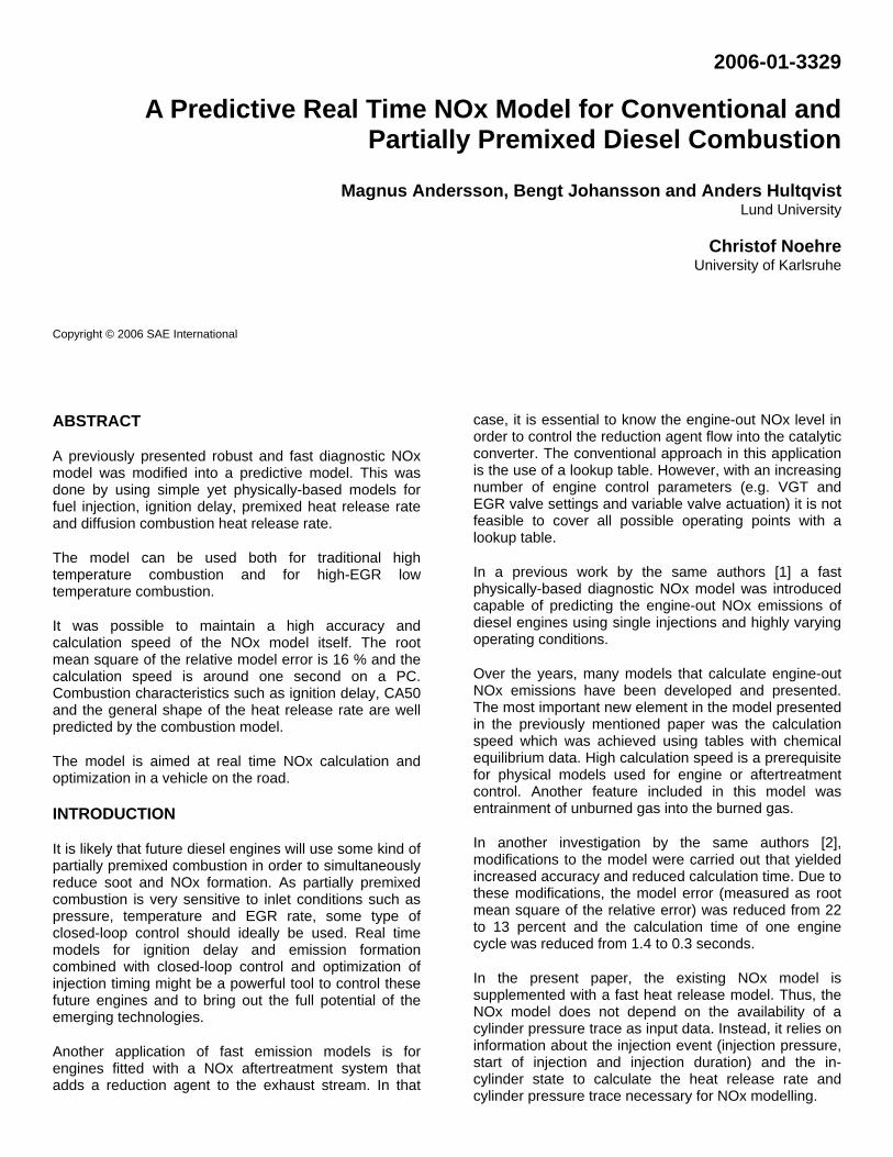
Premixed combustion

The shape of the premixed heat release is modeled semi-empirically as a Gauss curve (see Figure 3), whereas the amount of premixed combustion (the area under the curve) is physically modeled. The peak of premixed combustion, i.e. the peak of the Gauss curve, is assumed to occur 1.5 standard deviations after time of ignition; or, in other words, the time of ignition is defined as occurring 1.5 standard deviations before the premixed spike.

To determine the shape of the Gauss curve, we assume that the conditions that promote fast premixed combustion are similar to the conditions that promote short ignition delay. Therefore, a similar Arrhenius approach as the one for ignition delay is used:

TTk

aO

bapremprem

i

exkR⋅−

+ ⋅⋅⋅=2

222ρ (10)

A high value of Rprem at the time of ignition means high premixed heat release rate and short duration of premixed heat release.

355 356 357 358 3590

50

100

150

200

250

300

350

CAD

Pre

mix

ed H

eat R

elea

se R

ate

[J/C

AD

]

Figure 3. Premixed heat release rate as a function of CAD. Fast heat release (solid blue line) and slow heat release (dashed magenta line) with identical total premixed heat release (area under curve). Time of ignition marked with red dots.

The standard deviation (in CAD) of the Gauss curve is calculated:

premprem R

rpm⋅=

6σ (11)

Now, the amount of premixed combustion should be calculated. According to Siebers [7 and 8], the following relation holds for air entrainment into a diesel spray:

( ) ffaa uxDxm ⋅⋅⋅⋅∝ ρρ& (12)

where ρa is density of entrained cylinder gas and x is distance from injector. Thus the flow rate of entrained cylinder gas at any axial distance in one fuel spray can be calculated:

( ) ffaentraina uxDCxm ⋅⋅⋅⋅⋅= ρρ& (13)

where Centrain is an air entrainment constant. For simplicity, no correction is made for the spray/wall interaction that occurs at long axial distances. At each axial distance from the injector, the relative air/fuel ratio can be calculated:

stoichf

a

f

a

mm

mxm

x

⎟⎟⎠

⎞⎜⎜⎝

⎛=

&

&

&

& )(

)(λ (14)

where the mass flow rate of fuel at any axial location in the spray is the injected mass flow rate calculated by Equation 4. The stoichiometric air/fuel ratio is easily calculated if the species concentrations of the cylinder

gas are known. For calculation of species concentrations, see [1]. By applying the law of momentum conservation

( ) )()( xuxmmum sprayafff ⋅+=⋅ &&& (15)

the position of each fuel element in time and space (x axis location) can be calculated. Figure 4 shows how time (CAD after a fuel element was injected), axial location and local lambda are interrelated. For example, for the current in-cylinder conditions, 3 CADs after being injected, a fuel element has reached 40.4 mm and has mixed with cylinder gas to reach a local lambda of 0.45. At that lambda, the heat release fraction is 0.37, which means that if premixed burn occurs at that moment, the current fuel element will release 37 % of its lower heating value. The heat release fractions as a function of lambda were taken from a figure presented in [9]. It was found that the heat release fraction increases virtually linearly with local lambda up to λ=1. At higher values of lambda, the heat release fraction is unity. It was assumed that no heat release will occur where the mixture is richer than λ=0.2. Finally, the amount of premixed heat release is calculated by integrating the heat release fraction over the amount of fuel at each axial location. This is done at the CAD when the premixed spike is predicted to occur.

0 0.01 0.02 0.03 0.04 0.050

0.5

1

HR

frac

tion

& L

ambd

a

Axial distance from nozzle [m]

Local LambdaHeat Release FractionPremixed Heat Release

0 0.01 0.02 0.03 0.04 0.05

-0.01

0.011 CAD

2 CAD 3 CAD 4 CAD

Axial distance from nozzle [m]

Rad

ial d

ista

nce

[m]

Figure 4. Time (CAD after a fuel element was injected), axial location, local lambda and local heat release fraction in the fuel spray.

The approach to calculate premixed combustion described above might seem overambitious for a fast NOx model. However, the present combustion model should ideally be compatible with a future fast soot model; for a soot model it is essential to know the air/fuel ratio and temperature of each gas element and it is therefore essential to know approximately the air/fuel ratio of each fuel element at the start of combustion.

Diffusion combustion

Diffusion combustion is generally considered as mixing controlled and according to Chmela et al. (6), the diffusive heat release rate can be calculated:

dilutedstoich

stoichdiff

diff

aa

lkmLHVC

dtdQ

_mod ⋅⋅⋅⋅= (16)

where Cmod is a model constant, LHV is the Lower Heating Value of the fuel, mdiff is fuel mass available for diffusive combustion, k is density of turbulent kinetic energy [m2/s2], l is a characteristic length [m], astoich is stoichiometric air/fuel ratio and astoich_diluted is stoichiometric gas/fuel ratio (where gas refers to air and burned gas in the cylinder). The fuel mass available for diffusive combustion, mdiff, is calculated as the difference between the fuel injected up to any point in time and the fuel burnt:

LHVQmm injFdiff −= , (17)

According to Chmela, the characteristic length is a measure of the distance between molecules which changes due to compression and expansion and is calculated:

3cylVl = (18)

where Vcyl is current cylinder volume. This approach was tested by the authors of the present paper but found unable to correctly reflect the heat release rate during strong variations in dilution by EGR (which means strong variations of astoich_diluted). Instead, an attempt was made to include the effect of charge dilution in the calculation of the mixing length:

31

OA cNl

⋅= (19)

where NA is Avogadro’s Number and cO is oxygen gas concentration [mole/m3]. The physical meaning of this length is the mean distance between oxygen molecules. Now Equation 16 can be simplified:

lkmLHVC

dtdQ

diffModdiff ⋅⋅⋅= (20)

Equation 20 combined with 19 turned out to yield excellent predictions of heat release rate even at highly varying rates of charge dilution.

Chmela et al. assumed that all turbulent kinetic energy was generated by the spray; this is only realistic if the combustion chamber can be considered as quiescent. In

the model of the present paper, the turbulent kinetic energy is therefore divided into two parts, the first generated by the spray and the second by the in-cylinder swirl:

swirlspray kkk += )()( ττ (21)

At high injection pressure, low swirl number and low rpm, spray generated turbulence dominates; at low injection pressure, high swirl number and high rpm, swirl generated turbulence dominates. The density of spray generated turbulence is calculated:

AEOIfadeCOturbsprayspray exPCk ττ ⋅−⋅⋅∆⋅=

2_)( (22)

where Cspray_turb is a constant, Cfade is a constant governing the half time of spray generated turbulence due to dissipation and τAEOI is the time after end of injection. The density of swirl generated turbulence is calculated:

( )2_ BrpmRCk sturbswirlswirl ⋅⋅⋅= (23)

where Cswirl_turb is a constant, Rs is the swirl ratio and B is cylinder bore.

Transition from premixed to diffusive combustion

To achieve a smooth and realistic transition from premixed to diffusive combustion, an entirely empirical approach is taken: the diffusive heat release rate calculated by Equation 20 is multiplied by a ‘ramp’ factor that increases linearly from zero, at two standard deviations (as defined by Equation 11) before the premixed spike, to one, at four standard deviations after the spike. Then the diffusive heat release rate at all CADs is normalized so that the total diffusive heat release is unchanged.

Tuning the calibration parameters of the heat release model

The value of the heat radiation constant Crad was taken over from the diagnostic NOx model [1], where it had been tuned to yield the correct average NOx emission.

The amount of injected fuel according to the model must equal the measured amount of injected fuel; this is done by calibrating Cc in Equation 4.

In the expression for ignition delay (Equation 9), density can be varied by altering the intake pressure, which gives a value of a+b. Oxygen fraction is varied by altering the EGR rate, which gives a value of a. Temperature is varied by changing the intake temperature (or by increasing compression ratio, while simultaneously decreasing intake pressure), which gives a value of k2·Ti. The constants k2 and Ti cannot be

separated if only one fuel is tested such as in the present case.

The three constants of Equation 10, that control the shape of the premixed heat release, are tuned in a similar way as the ones in Equation 9 as described in the previous paragraph.

The air entrainment constant Centrain is tuned to give a correct amount of premixed heat release.

In the equation for diffusive heat release rate (Equation 20) CMod is tuned to give a correct diffusive heat release rate.

The relation between Cspray_turb and Cswirl_turb is given by varying engine speed and/or injection pressure. The model should give a correct diffusive heat release rate in spite of this variation. The constant Cfade is tuned to correctly reflect the fading of diffusive heat release rate after the end of injection. This is ideally done at low engine speed and high injection pressure.

CONNECTING HEAT RELEASE MODEL TO NOX MODEL

The formation of combustion products (input for NOx model) is calculated from the heat release rate assuming that all fuel is combusted at a fuel/air equivalence ratio of one. This is in agreement with modern theory of diffusion flames in general and of diesel combustion in particular [10]. However, this a substantial simplification of the real combustion process of both conventional and partially premixed diesel combustion, especially when the premixed part of combustion is large. The effect of this difference between real and modeled combustion is that there will sometimes be a time lag between model and reality concerning when elements of burned gas have reached equivalence ratio one.

The NOx model also requires the cylinder pressure as input data. The cylinder pressure is calculated by rearranging the first law of thermodynamics:

⎟⎠⎞

⎜⎝⎛ −⎟⎟⎠

⎞⎜⎜⎝

⎛−

−=Vd

dVpddQ

ddp n 1

1γ

ϕγγ

ϕϕ (24)

where Qn is net heat release and γ is ratio of specific heats, which is dynamically calculated depending on current in-cylinder temperature and composition.

ENGINE MEASUREMENTS FOR VALIDATION

For validation of the model, measurements from a single cylinder research engine based on a 6 cylinder truck engine were used. The engine was equipped with a common rail injection system. The rail pressure was 1500 bar. It was run at three different compression ratios (between 12.2:1 and 17.3:1), each with a different piston crown design providing three different combustion

chamber geometries. A very wide EGR range was used on these operating points (from 3 % up to 75 %) and combustion was in some cases conventional diesel diffusion type and in other cases (high EGR) partially premixed. However, due to limitations in the dynamometer control and engine vibrations, only a limited speed range could be tested (1100 – 1400 rpm). The single cylinder engine and the operating points used in this paper are identical to the single cylinder engine and its operating points used in [1]. For more details about the engine and the operating points please refer to the Appendix of that paper.

RESULTS

IGNITION DELAY

The ability of the heat release model to predict ignition delay is shown in Figure 5.

0

5

10

0 5 10

Measured Ignition Delay [CAD]

Pred

icte

d Ig

nitio

n D

elay

[CA

D]

Figure 5. Predicted vs. measured ignition delay at 42 operating points.

The coefficient of variation of the error in ignition delay predictions is 16 %.

HEAT RELEASE RATE

The predicted rates of premixed and diffusive heat release for a high compression ratio low-EGR operating condition are shown in Figure 6, and their sum, the total heat release, can be compared to the actual heat release rate which is calculated using the measured cylinder pressure trace.

355 360 365 370 375 380 385 3900

50

100

150

200

250

300

350

400

450

CAD

Hea

t rel

ease

rate

[J/C

AD

]

Premixed heat rel.Diffusive heat rel.Total heat rel.Measured heat rel.

Figure 6. Premixed, diffusive and total heat release rates and measured heat release rate for a low-EGR operating condition.

The corresponding heat release rates for a low compression ratio high-EGR operating condition are shown in Figure 7.

355 360 365 370 375 380 385 3900

50

100

150

200

250

300

350

CAD

Hea

t rel

ease

rate

[J/C

AD

]Premixed heat rel.Diffusive heat rel.Total heat rel.Measured heat rel.

Figure 7. Premixed, diffusive and total heat release rates and measured heat release rate for a high-EGR operating condition.

The general trends are captured when comparing predicted and measured (calculated using a single-zone heat release analysis of measured cylinder pressure data) heat release rates. The accuracy of CA50 predictions are shown in Figure 8. The standard deviation of the error in CA50 predictions is 1.0 CAD.

355

360

365

370

375

380

355 360 365 370 375 380

Measured CA50 (ATDC)

Pred

icte

d C

A50

(ATD

C)

Figure 8. Predicted vs. measured CA50 at 42 operating points.

NOX EMISSIONS

The results of the model compared to measured engine-out NOx levels at three different compression ratios (17.3, 14.5 and 12.2) are shown in Figure 9.

0

500

1000

1500

2000

0 500 1000 1500 2000

Measured engine-out NOx [PPM]

Pred

icte

d en

gine

-out

NO

x [P

PM] High CR

Medium CR

Low CR

Figure 9. Predicted vs. measured engine-out NOx.

Figure 9 shows operating points where the engine-out NOx level was above 100 ppm. At lower NOx levels (which occur at operating points with high EGR rates and thus lower combustion temperatures), the accuracy of the model was initially very poor as shown in Figure 10. This was to be expected as only the Zeldovich mechanism was used to model NOx formation even though other mechanisms are important at low temperatures as discussed above.

0

20

40

60

80

100

0 20 40 60 80 100Measured engine-out NOx [PPM]

Pred

icte

d en

gine

-out

NO

x [P

PM] High CR

Medium CR

Low CR

Figure 10. Predicted vs. measured engine-out NOx (without correction) at low-NOx operating points (high EGR, low temperature combusiton).

As in previous papers by the same authors [1 and 2], a simple empirical correction algorithm was applied at the end of each engine cycle to all burned zones with a NOx formation of less than 60 ppm:

43.0)(8.11 uncorrcorr ppmNOppmNO ⋅= (25)

The resulting NOx levels of the low-NOx operating points are shown in Figure 11.

0

20

40

60

80

100

0 20 40 60 80 100Measured engine-out NOx [PPM]

Pred

icte

d en

gine

-out

NO

x [P

PM] High CR

Medium CR

Low CR

Figure 11. Predicted vs. measured engine-out NOx (including empirical correction) at low-NOx operating points.

It is difficult to give an explanation for how the high accuracy of the low-NOx correction algorithm relates to the physics of NOx formation. However, to give the reader an idea of the temperature range where a correction is required, Figure 12 shows measured and predicted engine-out NOx vs. calculated values of maximum local temperature during the cycle; according to the figure it is obvious that the extended Zeldovich

mechanism alone can account for all NOx formation down to a temperature of approximately 2300 K. Below that temperature, one or several of the low-temperature mechanisms become important (predicted uncorrected values depart from measured values); these mechanisms were listed above.

0.1

1

10

100

1000

10000

1800 2000 2200 2400 2600 2800

Maximum local temperature [K]

Engi

ne-o

ut N

Ox

[PP

M]

Measured

Predicted (corrected)

Predicted (uncorrected)

Figure 12. Engine-out NOx vs. calculated maximum local temperature.

The root mean square of the relative error in the predicted engine-out NOx emissions was 16 %. The corresponding error of the diagnostic (i.e. based on pressure trace) version of the same NOx model was 13 % [2].

CALCULATION SPEED

The calculation time of one engine operating cycle is one second on a 2.8 GHz PC. The diagnostic version of the same model had a calculation time of 0.3 seconds [2]. One second computational time is not sufficient to handle engine transients. However, it would be possible to identify time-consuming calculation processes in the model and allocate them to an Application Specific Integrated Circuit (ASIC) and thus drastically decrease the required calculation time. For example, it has been shown that a net heat release calculation can be implemented on a re-programmable ASIC called Field Programmable Gate Array (FPGA) with a calculation time of only 70 µs per engine cycle [11]; put in different words, at 1200 rpm, the FPGA could perform the complete heat release calculation 1400 times during the time it takes to complete one engine cycle. Therefore it seems reasonable to assume that if time-consuming calculation processes are allocated to an ASIC, the model should be sufficiently fast to handle engine transients.

SUMMARY AND CONCLUSION

A previously presented robust and fast diagnostic NOx model was modified into a predictive model.

Ignition delay is modeled based on an Arrhenius type expression.

Premixed heat release rate is assumed to follow the shape of a Gauss curve. The amount of premixed heat release is determined by simple jet theory.

The diffusive combustion is assumed to be mixing controlled and its heat release rate is given by a formulation involving turbulent kinetic energy (from spray and swirl) and a characteristic length. The characteristic length corresponds to the mean distance between oxygen molecules.

The model can be used both for traditional high temperature combustion and for high-EGR low temperature combustion.

It was possible to maintain a high accuracy and calculation speed of the NOx model itself. Combustion characteristics such as ignition delay, CA50 and the general shape of the heat release rate are well predicted by the combustion model.

The model is aimed at real time NOx calculation and optimization in a vehicle on the road. If combined with an engine efficiency model and a fast soot model, it would be possible to continuously optimize the diesel engine while driving.

As the present model is based on single injections only, it would probably need modifications before being applied on multiple-injection strategies, especially if there is a long time period between the first and the last injection.

ACKNOWLEDGMENTS

This work was financed by the Swedish Energy Agency.

REFERENCES

1. M. Andersson, B. Johansson, A. Hultqvist, C. Nöhre, “A Real Time NOx Model for Conventional and Partially Premixed Diesel Combustion”, SAE2006-01-0195.

2. M. Andersson, A. Hultqvist, B. Johansson, C. Nöhre, “Fast Physical NOx Prediction in Diesel Engines”, The Diesel Engine: The low CO2 and emissions reduction challenge (conference proceedings), Lyon, 2006.

3. S. R. Turns, “An Introduction to Combustion”, 2nd edition, McGraw-Hill, 2000.

4. P. Amnéus, F. Maus, M. Kraft, A. Vressner and B. Johansson, “NOx and N2O Formation in HCCI Engines”, SAE2005-01-0126.

5. G. Woschni, “A Universally Applicable Equation for the Instantaneous Heat Transfer Coefficient in the Internal Combustion Engine”, SAE670931.

6. F. Chmela, M. Engelmayer, G. Pirker and A. Wimmer, “Prediction of Turbulence Controlled

Combustion in Diesel Engines”, Proceedings of THIESEL 2004 Conference on Thermo- and Fluid Dynamic Processes in Diesel Engines, 2004.

7. D. Siebers, “Liquid-Phase Fuel Penetration in Diesel Sprays”, SAE980809.

8. D. Siebers, “Scaling Liquid-Phase Fuel Penetration in Diesel Sprays Based on Mixing-Limited Vaporization”, SAE1999-01-0528.

9. S. Kook, C. Bae, P. Miles, D. Choi and L. Picket, “The Influence of Charge Dilution and Injection Timing on Low-Temperature Diesel Combustion and Emissions”, SAE2005-01-3837.

10. J. Dec, "A Conceptual Model of DI Diesel Combustion Based on Laser-Sheet Imaging", SAE970873.

11. C. Wilhelmsson, P. Tunestål and B. Johansson, “Model based engine control using ASICs: A virtual heat release sensor”, Les Rencontres Scientifiques de l’IFP: “New Trends in Engine Control, Simulation and Modelling”, Rueil-Malmaison, 2006.

CONTACT

magnus.andersson@vok.lth.se

NOTATION AND ACRONYMS

a empirical exponent [-] a2 empirical exponent [-] b empirical exponent [-] b2 empirical exponent [-] cF fuel concentration [mole/m3] cO oxygen gas concentration [mole/m3] k density of turbulent kinetic energy [m2/s2] k1 model constant [m3/(mole·s)] k1b model constant [(mole/(m3·s))·(m3/kg)a+b] k1c model constant [(mole/(m3·s))·(m3/kg)a+b] k2 model constant [-] kprem model constant [(mole/(m3·s))·(m3/kg)a+b] kspray turbulent kinetic energy from spray [m2/s2] kswirl turbulent kinetic energy from swirl [m2/s2] l characteristic length [m]

am& gas entrained into spray [kg/s] mdiff fuel mass for diffusive combustion [kg]

fm& injected fuel mass rate [kg/s] mF,inj injected fuel mass [kg] nholes number of injector holes p cylinder pressure [Pa]

ppmNO concentration of NO formed during cycle [-] uf fuel injection velocity [m/s] uspray velocity of fuel and entrained gas [m/s] x distance from injector [m] xF molar fraction of fuel xO molar fraction of oxygen gas B cylinder bore [m] Cc coefficient of contraction [-] Cd discharge coefficient [-] Centrain model constant [-] Cfade model constant [1/s] Cmix model constant [CAD] Cmod model constant [-] Crad model constant [J/(mol·K4)] Cspray_turb model constant [m3/kg] Cswirl_turb model constant [-] D diameter of injector holes [m] K threshold value [mole/m3] LHV lower heating value [J/kg] NA Avogadros number [6.022 · 1023] Q heat released [J] Qn net heat released [J]

radQ& radiative heat transfer [J/s] R formation rate of radicals [mole/m3s] Rprem formation rate of radicals [mole/m3s] Rs swirl ratio [-] Tad adiabatic combustion temperature Tchar characteristic mixing time [CAD] T local charge temperature [K] Ti activation temperature [K] Vcyl current cylinder volume γ ratio of specific heats [-] ϕ crank angle [CAD] λ relative air/fuel ratio ρ charge density [kg/m3] ρa density of entrained gas [kg/m3] ρf liquid fuel density [kg/m3] τ time [s] τAEOI time after end of injection [s]

∆P pressure difference between rail and cylinder CA50 Crank angle when 50% heat is released CAD Crank Angle Degree EGR Exhaust Gas Recirculation PPM Part Per Million SOC Start Of Combustion VGT Variable Geometry Turbine