79th EAGE Conference & Exhibition 2017 Paris, France, 12-15 June 2017

Th A1 08

A Practical Tool for Simultaneous Analysis of 4D Seismic

Data, PEM and Simulation Model

A. Briceño* (Heriot-Watt University), C. MacBeth (Heriot-Watt University), M.D. Mangriotis

(Heriot-Watt University)

Summary

One of the main focuses of the geoscience industry is to constrain reservoir models to 3D and 4D seismic data

using quantitative workflows that are suitable for model updating and history matching. Seismic history

matching (SHM) closes the loop and minimizes the misfit between the observed 4D seismic and that predicted

by the reservoir model. A key problem in formulating this misfit function is a lack of understanding as to how

uncertainties in the seismic data, petroelastic model and simulation model interact. This can lead to lengthy and

time consuming workflows. This study presents a simple and interactive way of visualizing these uncertainties

whilst optimizing the SHM. The approach is applied initially to a synthetic example, and then to two different

field datasets from the UKCS and Norwegian Sea. The results demonstrate that qualitative updates can be

successfully applied to the simulation model in the presence of uncertainty in the PEM and noise in the 4D

seismic data.

79th EAGE Conference & Exhibition 2017 Paris, France, 12-15 June 2017

Introduction

The growth of history matching involving not only production data but also 4D seismic data is a very active field (Gosselin et al. 2003; Roggero et al. 2007). This integration helps to reduce the uncertainty of the final reservoir model solutions and improve the reliability of production forecasts (Walker 2006). Seismic history matching (SHM) closes the loop and minimizes the misfit between the observed data and that predicted by the reservoir model. This workflow relies on the petroelastic model (PEM) when computing the synthetic seismic from the simulated pressure and saturation changes. Many previous studies have pointed out the difficulty of selecting a PEM, the challenges in calibrating the model to the in situ response, and in particular the uncertainties involved. This non-uniqueness in the PEM, together with data and model uncertainties creates the need for time-consuming comparisons in the SHM workflow. This study presents a simple and interactive way of visualizing all of these uncertainties, whilst optimizing the SHM. The approach is illustrated by application initially to synthetic data and then to two different fields from the UKCS and Norwegian Sea.

Methodology

Our approach consists of a simple cross-plot of all changes in water saturation and pore pressure between the two time periods of interest in the reservoir history (usually pre-production baseline and a monitor). An example of this cross-plot is shown in Figure 1. The position of each point is defined by the simulation model predictions. Simulation models with a different selection of history matching parameters such as fault transmissibility multipliers, porosity multipliers, barrier locations, will have different simulation predictions and hence population of points on the cross-plot. Next, each point on the cross-plot is colour-coded according to the polarity of the 4D seismic signature. The input 4D seismic data are in the form of a difference between maps for the monitor and baseline data. For the applications we have chosen for an oil-water system (i.e. no gas), pressure increase softens the reservoir and gives the opposite polarity to water saturation increase or reservoir hardening via pressure depletion. Finally, the PEM can be overlain on top of this cross-plot by recognizing the result of Alvarez and MacBeth (2013), who proposed a proxy for the PEM

PCSwCA PS ∆−∆=∆ (1)

where CS and CP the only two parameters required, and which provide the balance between the relative contributions of saturation (∆Sw) and pore pressure (∆P) change to the overall time-lapse seismic signature (∆A). The PEM is now defined as a straight line ∆A = 0 passing through the origin of the cross-plot with the gradient CP/CS. From (1) it can be immediately observed that the line is a boundary that divides the cluster of points into two groups with different polarities. In practice the coefficients CP and CS are obtained by a calibration exercise, and if several equally-likely models are used then several lines need to be drawn on this plot. Thus the points are divided by a wide sector rather than single sharp boundary. Uncertainty in the seismic data is expressed by a change in the polarity of the points, which in turn changes the relationship with the PEM boundary. An incorrect simulation model changes the positions of the points which also changes the relationship to the PEM. In both cases the mismatch may be easily visualized for future corrective action.

79th EAGE Conference & Exhibition 2017 Paris, France, 12-15 June 2017

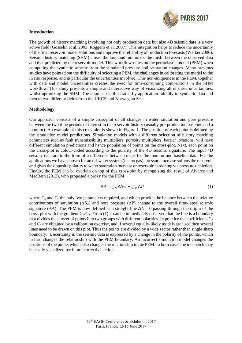
Figure 1 Schematic plot of ∆Sw versus ∆P from the simulation model, colour coded based on the polarity of the 4D response and with a selection of PEMs “a” to “d” overlain as straight lines. A red point corresponds to pressure increase, whilst blue is for water saturation increase.

Synthetic Example

The cross-plot is firstly applied to a synthetic 4D seismic dataset generated from a North Sea field model. The ∆P-∆Sw points are colour coded using the P-wave impedance, and are shown in Figure 2. Figure 2(a) gives the results for synthetic seismic calculated using a previously field-calibrated PEM A, and the boundary line relates to this model. Figure 2(b) gives the corresponding results for another model, PEM B. Both plots show a clear distinction and consistency between the two polarity groups.

Figure 2 Example of ∆Sw versus ∆P cross-plot, using P-wave impedances calculated from two different PEMS: (a) using the results from PEM A; (b) using the results from PEM B.

Observed Data Examples

The cross-plot is applied to two fields in the UKCS and Norwegian Sea with distinctly different geological settings. First of all, the ratio CP/CS for both fields are calculated using four different log calibrated deterministic PEMs (A, B, C and D) at baseline and monitor times following the work of Briceño et al. (2016). The ∆P-∆Sw cross-plot points are then colour-coded using the mapped 4D seismic amplitudes for both fields. For the UKCS field the seismic attribute chosen is sum of negative amplitudes (SNA), and for the Norwegian Sea field is root mean square (RMS). On top of our plots, we display the four different boundaries CP/CS obtained from the deterministic PEMs since they give a range of variability, and set the limits that represent softening and hardening of the reservoir.

∆P(MPa) (simulation model)

∆S

w(s

imul

atio

n m

odel

)Pressure build up

0

Saturation Dominates

Pressure Dominates

a bc

d

79th EAGE Conference & Exhibition 2017 Paris, France, 12-15 June 2017

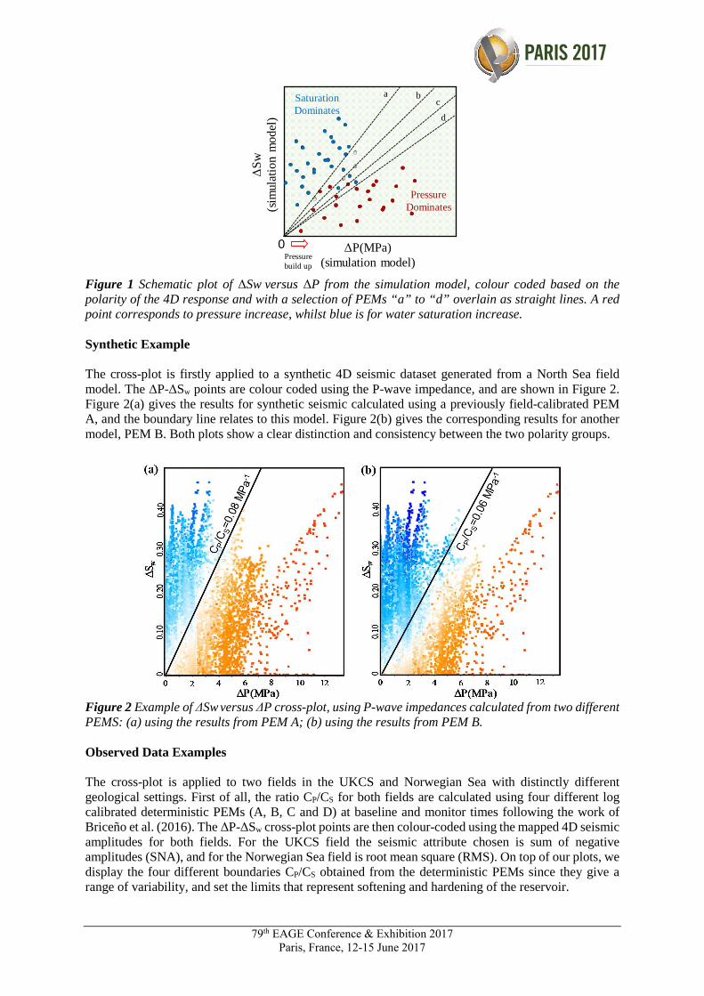
Figure 3 (a) Change in pore pressure map for 2004 minus baseline for our UKCS field. (b) Change in water saturation map. (c) 4D map using sum of negative amplitude attribute.

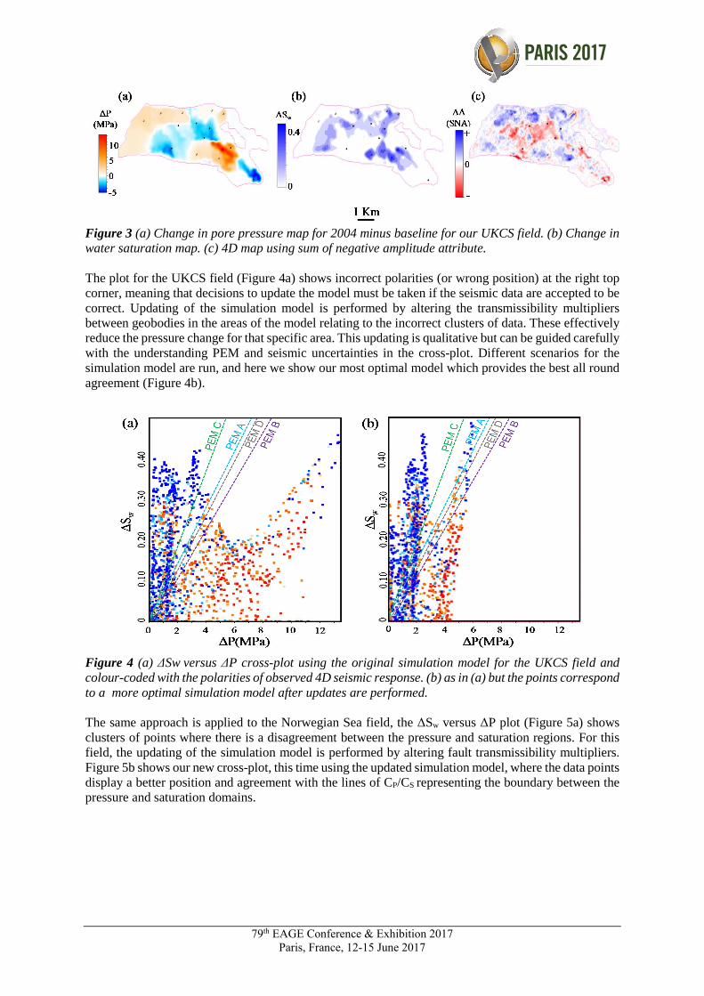
The plot for the UKCS field (Figure 4a) shows incorrect polarities (or wrong position) at the right top corner, meaning that decisions to update the model must be taken if the seismic data are accepted to be correct. Updating of the simulation model is performed by altering the transmissibility multipliers between geobodies in the areas of the model relating to the incorrect clusters of data. These effectively reduce the pressure change for that specific area. This updating is qualitative but can be guided carefully with the understanding PEM and seismic uncertainties in the cross-plot. Different scenarios for the simulation model are run, and here we show our most optimal model which provides the best all round agreement (Figure 4b).

Figure 4 (a) ∆Sw versus ∆P cross-plot using the original simulation model for the UKCS field and colour-coded with the polarities of observed 4D seismic response. (b) as in (a) but the points correspond to a more optimal simulation model after updates are performed.

The same approach is applied to the Norwegian Sea field, the ∆Sw versus ∆P plot (Figure 5a) shows clusters of points where there is a disagreement between the pressure and saturation regions. For this field, the updating of the simulation model is performed by altering fault transmissibility multipliers. Figure 5b shows our new cross-plot, this time using the updated simulation model, where the data points display a better position and agreement with the lines of CP/CS representing the boundary between the pressure and saturation domains.

79th EAGE Conference & Exhibition 2017 Paris, France, 12-15 June 2017

Figure 5 (a) ∆Sw versus ∆P cross-plot using the original simulation model for the Norwegian Sea field and colour-coded with the polarities of the observed 4D seismic response. (b) as in (a) but the points correspond to the best simulation model after updates are performed.

Conclusions

The ∆Sw-∆P cross-plot is found to be a simple yet effective tool to simultaneously visualize the uncertainties associated with three different domains: the simulation model, the seismic data and the PEM. The plot allows us to discriminate between regions in the reservoir that are dominated by pressure or saturation change using a straight-line boundary corresponding to the selected PEM. A synthetic example has verified the usefulness of this approach, and the sensitivities to both data and the model. Application to two field datasets has confirmed the utility of the cross-plot as a way of guiding updating of the simulation model to agree with the observed seismic data. This interactive method is useful as a step prior to a full quantitative seismic history matching.

References

Alvarez E., and MacBeth C. [2013] An insightful parametrization for the flatlander’s interpretation of time-lapse data. Geophysical Prospecting. 62, 75-96.

Briceño A., MacBeth C. and M.D. Mangriotis. [2016] Towards an effective petroelastic model for simulator to seismic studies. 78th EAGE Conference and Exhibition, Extended Abstracts, Th LHR2 08.

Gosselin O. Aanonsen S.I., Aavastmark I., Cominelli A., Gonard R., Kolasinski M., Ferdinandi F., Kovacic L., and Neylon K. [2003] History matching using Time-lapse Seismic (HUTS). SPE 84464. SPE Annual Technical Conference and Exhibition. Denver, Colorado, USA. DOI: 10.2118/84464-MS.

Roggero F., Ding D.Y., Berthet P., Lerat O., and Schreiber P.E. [2007] Matching of Production History and 4D Seismic Data – Application to the Girassol Field, Offshore Angola. SPE 109929. SPE Annual Technical Conference and Exhibition. Anaheim, California, USA. DOI: 10.2118/109929-MS.

Walker, G., Allan, P., Trythall, R., Parr, R., Marsh, M., Kjelstadli, R., Barkved, O., Johnson, D. and Lane, S. [2006] Three case studies of progress in quantitative seismic-engineering integration. The Leading Edge, 25 (9), 1161-1166.