A Practical Method for Aggregating Economic Capital … · DECEMBER 2012 RISK PROFESSIONAL 1 QUANT PERSPECTIVES A Practical Method for Aggregating Economic Capital using a Gumbel

www.garp.org D E C E M B E R 2 0 1 2 RISK PROFESSIONAL 1

Q U A N T P E R S P E C T I V E S

A Practical Method for Aggregating Economic Capital

using a Gumbel CopulaBy Dr. Yimin Yang

inancial institutions typically calculate economic capital for different risks or business lines through separate processes. One approach for aggregating economic capital is to use a copula, and there is a new calibration method for a Gumbel copula that

possesses several advantages over a Gaussian copula. -

tions to measure and monitor risks across the entire organiza-

The risk metric serves as a common risk language, enabling comparisons of risk assessment outcomes. Having such a yard-

to perform risk analysis, engineer portfolio strategies and im-plement risk management actions.

Typical risk metrics include expected and unexpected loss (EL/UL), value-at-risk (VaR), economic capital (EC) and ex-pected shortfall or tail VaR (ES/TVaR). When implemented, the approaches and calculation methods of a risk metric can vary substantially from portfolio to portfolio or business unit to business unit.

Certain metrics, such as EL, are “linear” in nature, so its computation is usually straightforward. However, “non-linear”

challenges. These include not only increasing computation complexity at an individual quantitative model level, but also the lack of adequate methodologies and approaches for the aggregation and attribution of risks when multiple portfolios and/or product segmentations are involved.

The purpose of this article is to present an example for the aggregation of EC using a Gumbel copula. We introduce a new calibration method and demonstrate it through commer-

cial and retail credit losses. The main advantage of this method is simplicity in implementation. It also avoids some undesirable features of the common Gaussian copula.

Economic Capital

-pectations. It is normally associated with a preset loss tolerance

of the loss distribution. Ideally, EC should be calculated using one single-loss model

that is responsive to all risk factors and covers all products in -

velop separate loss models based on their business nature and their product segmentations. For example, banks typically per-form two individual EC calculations: one for the commercial portfolio and one for the retail portfolio.

EC numbers are normally obtained through simulation models that simulate future loss scenarios and generate loss tails. However, due to its “non-linear” nature (often referred to

-folio cannot be aggregated directly. In fact, without performing another layer of modeling and calculation, knowing the EC

determine the combined EC. This additional calculation layer is commonly referred to as risk aggregation.

Risk Aggregation

As most risk metrics measure tail losses, an appropriate risk ag-gregation framework is fundamental in obtaining a meaningful, high-level risk assessment.

There are four common approaches (including their varia-tions) for calculating the combined loss distribution tail. One is

F

2 RISK PROFESSIONAL D E C E M B E R 2 0 1 2 www.garp.org


the use of direct simulation. For example, market risk VaR for a trading portfolio is often derived using multifactor stochastic simulations.

The second approach makes use of certain assumptions re-

-ing distribution using central limit theorem (CLT) or extreme value theorem (EVT).

The third approach uses various approximations (such as Delta-Gamma, Cornish-Fisher and Saddle Point approxima-tion), while the last approach for risk aggregation (which is also

What is a Copula?

The word “copula” is of Latin origin, meaning “connection.” In mathematics, it is used to describe the dependence between random variables. Technically, a copula is a tool that expresses joint probability function as a function of marginal distributions.

In the two-dimensional case, a copula between two random variables, X and Y, is a function C(u,v) from [0,1]×[0,1] [0,1], such that

Prob{X<x, Y<y} = C(F(x), G(y)),

where F(x) = Prob{X<x } and G(y) = Prob{Y<y} are cumulative distribution functions.

The usefulness of copulae can be seen in the groundbreaking work by Sklar (Sklar’s Theorem, 1959), as follows:

Let F be an n-dimensional cumulative distribution function with mar-ginal distributions F1, …, Fn. Then there is a copula function C, such that

Prob{Xn<x1, ……, Xn<xn} = C(F1(x1),……, Fn(xn)).

Roughly speaking, the theorem asserts that any relationship between any random variables can be captured by a copula.

Copula Classes, and Lessons Learned from the

Recent Financial Crisis

Although a wide range of copulae exist, two types are most

the popular Gaussian and Student-t copulae. The second type is the Archimedean class, which contains, among others, the Clayton, Gumbel and Frank copula families.

An n-dimensional elliptical distribution X is of the following form:

X = µ +RAU,

where µ is an n-dimensional mean vector, An×k is an n×k matrix, U is a k-dimensional random vector uniformly distributed on the unit hypersphere

by the joint distribution function of X is an elliptical copula.

An Archimedean copula, meanwhile, takes the follow-

ing form:

Let ! be a continuous, strictly decreasing, convex function from [0, 1] to [0 ! !-1 be its pseudo-inverse, then C(u, v) = !-1(!(u) + !general, C(u1,…,uk) = !-1(!(u1)+…+ !(uk)) is a k-dimensional Archi-medean copula.

The Gaussian copula in the elliptical class is the most famous one. It has been widely used for many applications. In 2000, quantitative analyst David X. Li introduced a pricing model for collateralized debt obligations (CDO) using the Gaussian copula. It quickly became a market standard for its easy and intuitive calculation.

was criticized as a “recipe for disaster” for its lack of sensitiv-ity to stressed scenarios. However, in fairness, formulae do not cause losses. People, in particular the users, need to be aware of the shortcomings and the situations where formulae can break.

Throughout the years, the Archimedean copula (the second class) has also been the subject of numerous studies by aca-demic researchers. Its advantage is that the copula function C is explicitly given.

Our Copula Choice

The Archimedean copula is a very rich class with broad appli-cations. Our research shows that nearly countless copulae can be created through “generating functions.” For the purpose of risk aggregation, we are interested in a copula with the follow-ing characteristics: (1) compatibility with “fat tail” distributions

sensitive to large losses, but less sensitive to small losses); (2) sim-ple and robust parameter estimation methods; (3) familiarity with practitioners and regulators; and (4) easy to implement.

large losses tend to come as surprises – the “fat tail.” It rules out the elliptical class, as these copulae do not have fat tails. In the Archimedean class, the Clayton has a “thin tail” while the



Frank has “no tail.” Only the Gumbel has a “fat tail.” Math-ematically, the Gumbel copula function is given by

with ">1 being the parameter.The parameter " controls the behavior of the copula, in-

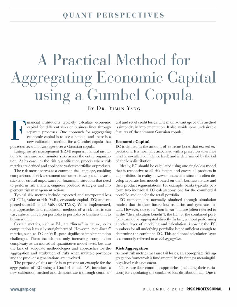
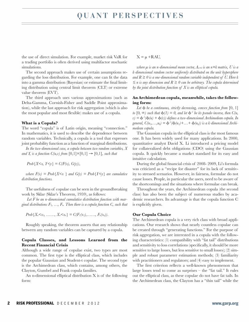
cluding the correlation between losses. Further investigation shows that this copula possesses a very desirable feature: heavi-er losses are associated with higher correlations (see Figure 2, below). This is in contrast to the constant correlation assump-tion with the Gaussian copula (see Figure 1, below).

Figure 1: The Gaussian Copula

Figure 2: The Gumbel Copula

Intuitively, when the situation is getting worse, things tend to go bad all together. So the Gumbel copula is a good candidate

-fects of the Gaussian and Gumbel copulae. The x and y-axis represent the loss severity quantiles of two random variables (the higher, the worse). The diagonal line exhibits the correla-tion effect. In Figure 1 (the Gaussian copula), both ends display similar patterns. In contrast, in Figure 2 (the Gumbel copula),

-relation.

standard statistical concepts.

Basic Statistics

Suppose X and Y are random variables with marginal distribu-tion functions F(x) and G(y). Let C(u,v) be the copula between X and Y, and let P be the probability measure, as follows:

#(X, Y) = P{(X – X* )(Y – Y* *)(Y – Y*

where (X* , Y*) is an independent copy of (X,Y).

Proposition

1) For the Gaussian copula: $ is the linear correlation between X and Y.

2) For the Clayton copula: The copula has only left tail.

3) For the Frank copula: The copula has no tails.

4) For the Gumbel copula: The copula has only right tail.

Let U and V be independent uniform distributions and let W=C(U,V). Prob {W<w}.

For the Gumbel copula, K(w)=Prob {W<w} = w- 1 w ln w.

An Archimedean copula, meanwhile, takes the following form:

Let be a continuous, strictly decreasing, convex function from [0, 1] to [0, ) such that (1)

= 0, and let -1 be its pseudo-inverse, then C(u, v) = -1( (u) + (v)) defines a 2-dimensional Archimedean copula. In general, C(u1,…,uk) = -1( (u1)+…+ (uk)) is a k-dimensional Archimedean copula.

The Gaussian copula in the elliptical class is the most famous one. It has been widely used for many applications. In 2000, quantitative analyst David X. Li introduced a pricing model for collateralized debt obligations (CDO) using the Gaussian copula. It quickly became a market standard for its easy and intuitive calculation.

During the global financial crisis of 2008- 2009, Li’s formula was criticized as a “recipe for disaster” for its lack of sensitivity to stressed scenarios. However, in fairness, formulae do not cause losses. People, in particular the users, need to be aware of the shortcomings and the situations where formulae can break.

Throughout the years, the Archimedean copula (the second class) has also been the subject of numerous studies by academic researchers. Its advantage is that the copula function C is explicitly given.

Our Copula Choice The Archimedean copula is a very rich class with broad applications. Our research shows that nearly countless copulae can be created through “generating functions.” For the purpose of risk aggregation, we are interested in a copula with the following characteristics: (1) compatibility with “fat tail” distributions and sensitivity to loss correlations (specifically, it should be more sensitive to large losses, but less sensitive to small losses); (2) simple and robust parameter estimation methods; (3) familiarity with practitioners and regulators; and (4) easy to implement.

The first criterion reflects a well-known phenomenon that large losses tend to come as surprises – the “fat tail.” It rules out the elliptical class, as these copulae do not have fat tails. In the Archimedean class, the Clayton has a “thin tail” while the Frank has “no tail.” Only the Gumbel has a “fat tail.” Mathematically, the Gumbel copula function is given by

with >1 being the parameter.

The parameter controls the behavior of the copula, including the correlation between losses. Further investigation shows that this copula possesses a very desirable feature: heavier losses are associated with higher correlations (see Figure 2, below). This is in contrast to the constant correlation assumption with the Gaussian copula (see Figure 1, below).

Figure 1: The Gaussian Copula

Basic Statistics Suppose X and Y are random variables with marginal distribution functions F(x) and G(y). Let C(u,v) be the copula between X and Y, and let P be the probability measure, as follows:

1. Kendall’s tau is defined as

(X, Y ) = P{(X – X* )(Y – Y* ) > 0} P{(X X* )(Y Y* ) < 0}, where (X* , Y* ) is an independent copy of (X,Y).

2. Upper tail dependence is defined as

3. Lower tail dependence is defined as

Proposition

1) For the Gaussian copula: Here, is the

linear correlation between X and Y.

2) For the Clayton copula: ,

The copula has only left tail.

3) For the Frank copula: ,

The copula has no tails.

4) For the Gumbel copula: ,

The copula has only right tail.

Definition and Proposition Let U and V be independent uniform distributions and let W=C(U,V). Define function

For the Gumbel copula,

Calibration Formulae Kendall’s and the function K(w) can be estimated when a set of data are observed. Specifically, suppose X and Y are random variables and is a set of observations, then we can make the following empirical estimations:

1) Kendall’s can be estimated by






Proposition


















Proposition


















Proposition


















Proposition


















Proposition


















Proposition


















Proposition













"



Calibration Formulae

Kendall’s # and the function K(w) can be estimated when a set X and Y are random

variables and {(xi ,yi)}i=1,... N is a set of observations, then we can make the following empirical estimations:

1) Kendall’s # can be estimated by

2) The function K(w) can be estimated by

Here

We state below our estimation method for the Gumbel copu-la’s parameter " based on K

^(w) (the second method). Its deriva-

tion is provided in the appendix.

Estimations for the Two-dimensional Gumbel Copula

The following steps can be used to estimate the Gumbel copula:

The last formula only applies to two-dimensional Copula – it is based on the minimal value of the quadratic polynomial: When the dimension , one can prove that the integral becomes a polynomial of degree 2(d-1). Although

formula is no longer available in general as there is no solution

An Example

Now let us use an example to demonstrate the EC aggrega-

tion process using the Gumbel copula. Suppose we work with a commercial and industrial (C&I) loan portfolio and a consumer

-cial institutions calculate EC for such portfolios through sepa-rate simulation processes.

Let’s also suppose LCI and LR are the simulated loss distributions for the C&I and the consumer portfolios, respectively (assum-ing expected losses are already deducted from the loss distribu-tions).

Ideally, one should use historical loss experience of these two portfolios to calibrate the Gumbel copula. However, such in-ternal data is generally not available, and we therefore have to explore external resources for a proxy.

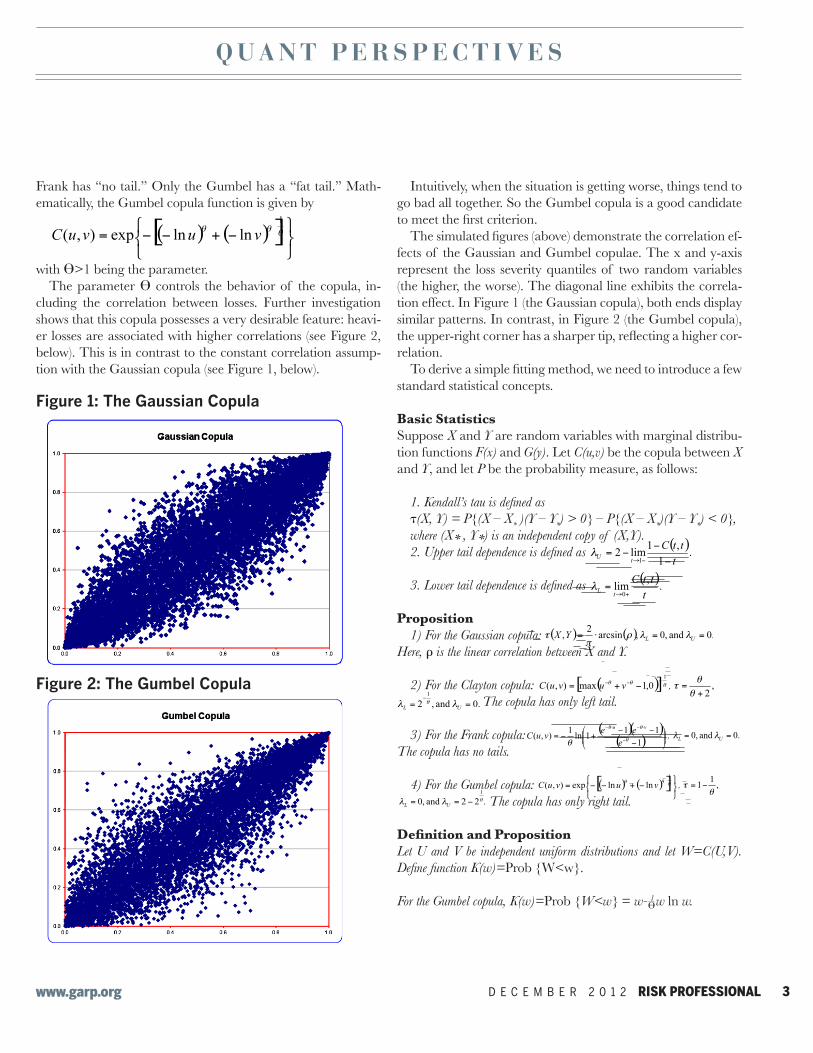
Government agencies such as the Federal Reserve publish bank loan losses on a quarterly basis. We use the Fed’s histori-

consumer loans (see Figure 3, below) to calibrate our copula.

Figure 3: Fed Historical Charge-offs

The Gumbel Copula Fitting Process

copula:1) Download and index the Fed data as {(xi,yi)}i-1,...N -

sents C&I charge-offs and y represents consumer charge-offs.2) Calculate zi , zi *, ki , ni , %*, #̂ , and "

^, as in the estimations for the

Gumbel copula that we reviewed earlier.The Fed data estimates #̂ =0.3123 and "

^=1.4102. For

benchmarking purposes, we also include #̂ here, and it provides another estimation of 1.4541 through "

^ = 1 .

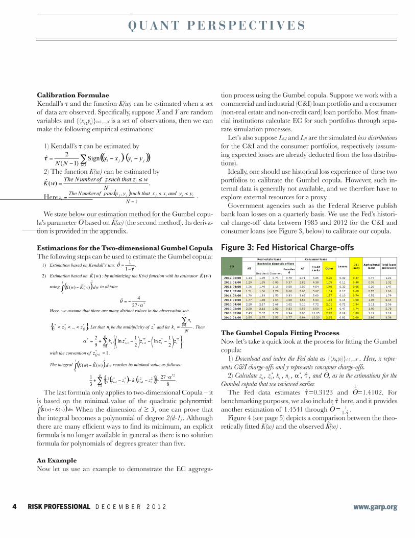
Figure 4 (see page 5) depicts a comparison between the theo-K(w) and the observed K

^(w) .






Proposition













6


Here .

We state below our estimation method for the Gumbel copula’s parameter based on

(the second method). Its derivation is provided in the appendix.

Estimations for the 2-dimensional Gumbel Copula The following steps can be used to estimate the Gumbel copula:

1) Estimation based on Kendall’s tau:

2) Estimation based on : by minimizing the K(w) function with its estimator

using to obtain:

Here. we assume that there are many distinct values in the observation set:

. Let that be the multiplicity of and let . Then

with the convention of .

The integral reaches its minimal value as follows:

.

The last formula only applies to 2-dimensional Copula – it is based on the minimal value of the

quadratic polynomial: . When the dimension d 3, one can prove that the

integral becomes a polynomial of degree 2(d-1). Although there are many efficient ways to find its minimum, an explicit formula is no longer available in general as there is no solution formula for polynomials of degrees greater than 5.

An Example Now let us use an example to demonstrate the EC aggregation process using the Gumbel copula. Suppose we work with a commercial and industrial (C&I) loan portfolio and a consumer (non-real estate and non-credit card) loan portfolio. Most financial institutions calculate EC for such portfolios through separate simulation processes.

6


Here .






using to obtain:





.





6


Here .






using to obtain:





.





6


Here .






using to obtain:





.





Let’s also suppose LCI and LR are the simulated loss distributions for the C&I and the consumer portfolios, respectively (assuming expected losses are already deducted from the loss distributions). Ideally, one should use historical loss experience of these two portfolios to calibrate the Gumbel copula. However, such internal data is generally not available, and we therefore have to explore external resources for a proxy. Government agencies such as the Federal Reserve publish bank loan losses on a quarterly basis. We use the Fed’s historical charge-off data between 1985 and 2012 for the C&I and consumer loans (see Figure 3, below) to calibrate our copula.

Figure 3: Fed Historical Charge-offs

The Gumbel Copula Fitting Process Now let’s take a quick look at the process for fitting the Gumbel copula:

1) Download and index the Fed data as . Here, x represents C&I charge-offs and y represents consumer charge-offs.

2) Calculate , , ki , ni , *, , and , as in the estimations for the Gumbel copula that we reviewed earlier..

The Fed data estimates and . For benchmarking purposes, we also

include here, and it provides another estimation of 1.4541 through .

Figure 4 (below) depicts a comparison between the theoretically fitted K(w) and the observed .

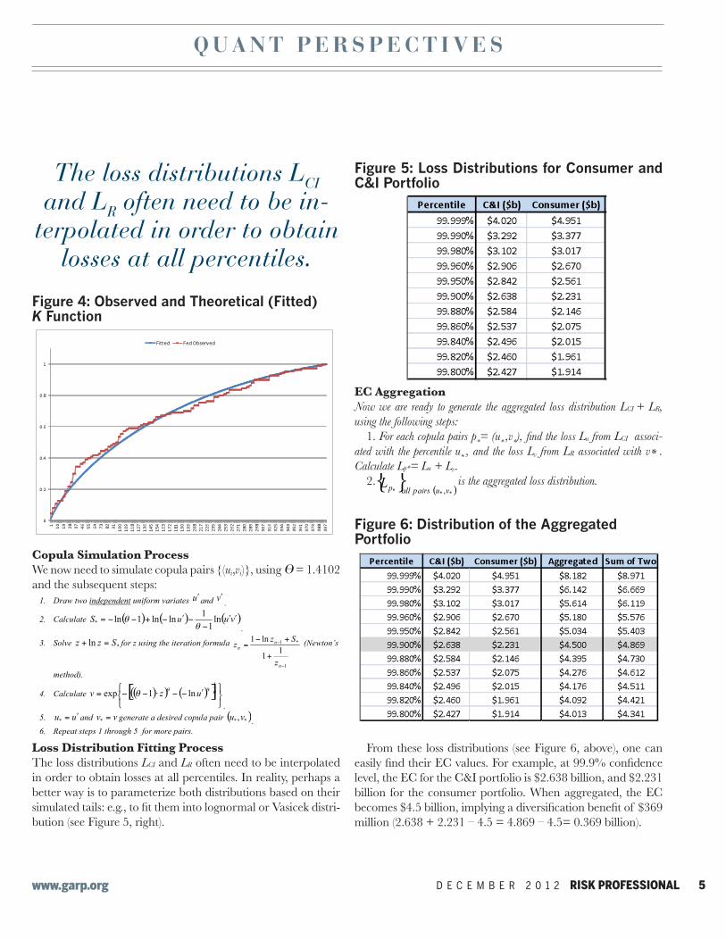
Figure 4: Observed and Theoretical (Fitted) K Function

1-#̂



Figure 4: Observed and Theoretical (Fitted) K Function

Copula Simulation Process

We now need to simulate copula pairs {(ui,vi)}, using " = 1.4102 and the subsequent steps:

Loss Distribution Fitting Process

The loss distributions LCI and LR often need to be interpolated in order to obtain losses at all percentiles. In reality, perhaps a better way is to parameterize both distributions based on their

-bution (see Figure 5, right).

Figure 5: Loss Distributions for Consumer and C&I Portfolio

EC Aggregation

Now we are ready to generate the aggregated loss distribution LCI + LR, using the following steps:

1. For each copula pairs p*= (u* ,v* u from LCI associ-ated with the percentile u* , and the loss Lv from LR associated with v* . Calculate Lp*= Lu + Lv.

2. is the aggregated loss distribution.

Figure 6: Distribution of the Aggregated Portfolio

From these loss distributions (see Figure 6, above), one can

billion for the consumer portfolio. When aggregated, the EC

1. Draw two independent uniform variates and .

2. Calculate .

3. Solve for z using the iteration formula (Newton’s

method).

4. Calculate .

5. and generate a desired copula pair .

6. Repeat steps 1 through 5 for more pairs.

The loss distributions LCI and LR often need to be in-

terpolated in order to obtain losses at all percentiles.

is the



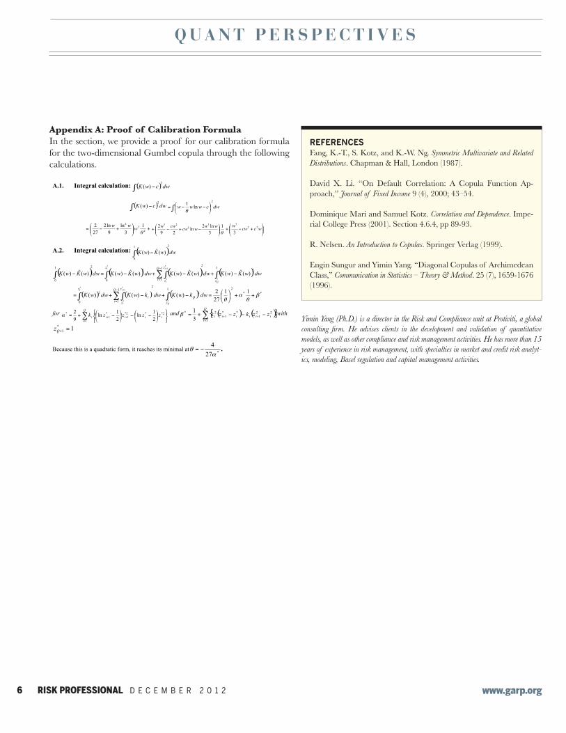
Appendix A: Proof of Calibration Formula

In the section, we provide a proof for our calibration formula for the two-dimensional Gumbel copula through the following calculations.

Yimin Yang (Ph.D.) is a director in the Risk and Compliance unit at Protiviti, a global

years of experience in risk management, with specialties in market and credit risk analyt-ics, modeling, Basel regulation and capital management activities.

REFERENCESFang, K.-T., S. Kotz, and K.-W. Ng. Symmetric Multivariate and Related Distributions

David X. Li. “On Default Correlation: A Copula Function Ap-proach,” Journal of Fixed Income 9 (4), 2000; 43–54.

Dominique Mari and Samuel Kotz. Correlation and Dependence. Impe-

R. Nelsen. An Introduction to Copulas. Springer Verlag (1999).

Engin Sungur and Yimin Yang. “Diagonal Copulas of Archimedean Class,” Communication in Statistics – Theory & Method(1996).

10

Appendix A: Proof of Calibration Formula In the section, we provide a proof for our calibration formula for the 2-dimensional Gumbel copula through the following calculations.

A.1. Integral calculation:

A.2. Integral calculation:

for and with

Because this is a quadratic form, it reaches its minimal at .

REFERENCES David X. Li. “On Default Correlation: A Copula Function Approach,” Journal of Fixed Income 9 (4), 2000; 43–54. Dominique Mari and Samuel Kotz. Correlation and Dependence. Imperial College Press, 2004” Section 4.6.4, pp 89-93. R. Nelsen. An Introduction to Copulas. Springer Verlag (1999). Engin Sungur and Yimin Yang. “Diagonal Copulas of Archimedean Class,” Communication in Statistics – Theory & Method. 25 (7), 1659-1676 (1996). Fang, K.-T., S. Kotz, and K.-W. Ng. “Symmetric Multivariate and Related Distributions,” Chapman & Hall, London (1987).

Documents

A Practical Method for Aggregating Economic Capital … · DECEMBER 2012 RISK PROFESSIONAL 1 QUANT PERSPECTIVES A Practical Method for Aggregating Economic Capital using a Gumbel