A Practical Implementation of Robust EvolvingCloud-based Controller with Normalized Data

Space for Heat-Exchanger PlantGoran Andonovski

Faculty of Electrical EngineeringUniversity of Ljubljana, Slovenia

goran.andonovski@fe.uni-lj.si

Plamen AngelovSchool of Coputing and Communications

Lancaster University, United Kingdomp.angelov@lancaster.ac.uk

Saso Blazic, Igor SkrjancFaculty of Electrical EngineeringUniversity of Ljubljana, Slovenia

saso.blazic@fe.uni-lj.si,igor.skrjanc@fe.uni-lj.si

Abstract—The RECCo control algorithm, presented in thisarticle, is based on the fuzzy rule-based (FRB) system namedANYA which has non-parametric antecedent part. It starts withzero fuzzy rules (clouds) in the rule base and evolves its structurewhile performing the control of the plant. For the consequent partof RECCo PID-type controller is used and the parameters areadapted in an online manner. The RECCo does not require anyoff-line training or any type of model of the controlled process(e.g. differential equations). Moreover, in this article we proposea normalization of the cloud (data) space and an improvedadaptation law of the controller. Due to the normalizationsome of the evolving parameters can be fixed while the newadaptation law improves the performance of the controller in thestarting phase of the process control. To assess the performanceof the RECCo algorithm, firstly an comparison study withclassical PID controller was performed on a model of a plateheat-exchanger (PHE). Tunning the PID parameters was doneusing three different techniques (Ziegler-Nichols, Cohen-Coonand pole placement). Furthermore, a practical implementationof the RECCo controller for a real PHE plant is presented.The PHE system has nonlinear static characteristic and a timedelay. Additionally, the real sensor’s and actuator’s limitationsrepresent a serious problem from the control point of view.Besides this, the RECCo control algorithm autonomously learnsand evolves the structure and adapts its parameters in an onlineunsupervised manner.

I. INTRODUCTION

Nowadays, control of nonlinear and complex processes isstill an active research topic. Besides changing circumstances,process dynamics and complexity of the processes the indus-trial markets require high and satisfactory performance of thecontroller. A local linear approximation of the process com-bined with the classical PID controller provides good resultsbut only in the neighborhood of the linearized operating pointwhile this approach is not suitable for the whole operatingrange of the nonlinear process.

To solve the problem of nonlinearity the authors in [1]presented a self-tuning method for a class of nonlinear PIDcontrol systems based on Lyapunov approach. Another schemein [2] is presented where the just-in-time learning techniqueis employed to predict the process dynamics and furthermore,the Lyapunov method for adapting the PID parameters isused. There are many other techniques and methods, for

example, in [3] an online adaptation of PID controller usingneural networks is proposed and in [4] the genetic algorithmfor finding the optimal PID parameters is applied. Also theparticle swarm optimization for tunning the parameters ofPID controller in [5] is used. Another type of PID controllersare Fractional Order PID (FO PID) controllers that performbetter than a classical PID-s [6] but require setting of twoadditional parameters. Similar to classical ones, tunning of thisparameters can be solved by solving an optimization problem[7], [8], [9].

Fuzzy systems represent control scheme which is developedto deal with the nonlinear processes and due to their powerfuladaptability and nonlinear modeling capability they are widelyused in many applications [10], [11], [12], [13], [14], [15],[16], [17]. The author of fuzzy sets/systems is Prof. Lotfi A.Zadeh who firstly introduced the theory in [18]. After Prof.Zadeh has introduced the theory of fuzzy sets, Mamdani in[19] published the first fuzzy model based control applica-tion on dynamic plant (a model of steam engine). Anotherfuzzy control system is Takagi-Sugeno (TS) fuzzy approachproposed in [20] that has attracted lots of attention afterthe publication. The wide popularity and usage of the fuzzycontrol systems is presented in [21] where a lot of fuzzycontrol schemes are discussed. Similar to TS fuzzy modelsa new Tensor product (TP) models were developed. One ofthe advantages of the TP models is that the linear matrixinequality (LMI)-based control design can be applied directlyto TP models. Recently, several process control solution usingTP models were proposed for different applications [22], [23],[24], [25].

Mamdani and TS fuzzy systems are made up of IF-THENfuzzy rules representing the local linear input/output relationsof a nonlinear system. The first part (IF) of the conditionalis termed the antecedent, and the second part (THEN) isthe consequent. Although, both TS and Mamdani are fuzzysystems, they have some differences, especially in the way howthe conditional part is defined. Both fuzzy systems – TS andMamdani – have a fuzzy antecedent part, while they differ inthe consequent part which has the form of a functional (oftenlinear) in the case of TS systems and a form of fuzzy logic in

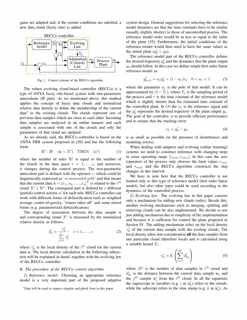
TABLE IA COMPARISON OF DIFFERENT TYPES OF FRB [26]

ANTECEDENT

(IF)

CONSEQUENT

(THEN)

DEFUZZI-

FICATION

Mamdani

[19]Fuzzy sets

(scalar, parame-

terized)

Fuzzy sets

(scalar, parame-

terized)

Center of

Gravity

TS

[20]

Functional

(often linear)

Fuzzily

weighted sum

ANYA

[26]

Data clouds

(non-parametric)

Any

of the above

two types

the case of Mamdani systems (see Table I).Besides the classical fuzzy rule-based (FRB) systems, TS

and Mamdani, Angelov and Yager proposed a new simplifiedtype of FRB system named ANYA in [26]. Moreover, theypresented a new concept how the antecedent part is defined.As we have already mentioned above in both classical FRBsystems the antecedent part is fuzzy and uses predefinedand fixed membership functions of triangular, trapezoidal,Gaussian type etc. ANYA FRB system extracts the informationfrom the real data and form the data clouds to define themembership function. The clouds are sets of data that havecommon properties (they are close to each other in the dataspace). All data have different degree of memberships to theexisting clouds determined by the local density of the datasample to all data from the particular cloud.

In [26] the authors distinguished between the clouds andthe clusters and they pointed out the main differences betweenthem. In general, the clouds do not require a priori informationabout the total number of membership functions or even anassumption about its form (do not have boundaries). More-over, data clouds represent all previous data samples that areassociated with the cloud.

Inspired and motivated by the simplicity of the ANYAFRB system several approaches on process control weredeveloped and tested on different simulation models [27],[28] and on a real plant [29]. Firstly, in [27] a new fuzzycontroller RECCo (Robust Evolving Cloud-based Controller)was introduced. The main advantage of the RECCo controlleris that it does not require any information and knowledge aboutthe controlled process (e.g. in a form of differential equations).Furthermore, it is initialized from the first data sample andlearns autonomously while performing the control of the plant.Also the structure of the RECCo is not predefined but evolvesin an online manner during the process control (adding newclouds – fuzzy rules). In [27] and [29] a new cloud is addedaccording to the global density of the data while in [28] and[30] a simpler way using local density threshold is proposed.Finally, controller’s parameters in the consequent part are alsotuned and adapted autonomously using stable gradient-basedlearning method.

In this paper we propose an improvement of the RECCocontroller presented in [28]. Our idea is by using the basicknowledge from the controlled process (input and outputrange, time constant and sampling time) to set/fix the initialparameters required by the algorithm. A new normalized dataspace is proposed and due to this the evolving parameterγmax can be fixed (γmax defines ’when’ a new cloud isadded and will be introduced later in more detail). Alsothe adaptation gain vector ααα could be calculated using therange of the control variable and the default value. Thusthe controller tuning is simplified which makes the approachmore appealing for the use in practical applications. Differentinitial real life scenarios were analyzed and new improvedadaptation law with absolute values in the starting phase isproposed to improve the performance of the controller [31].This improvement speed up convergence and reduce largetransients when the initial are far away from the unknownparameters.

In order to show the effectiveness of the proposed controller,we provide several experiments on a real plate heat-exchanger(PHE) plant and on a PHE model. Firstly, we comparedthe performance of the proposed algorithm RECCo with theclassical PID controller on PHE model. The parameters ofthe PID were tunned using Ziegler-Nichols [32], Cohen-Coon[33] and by pole placement method [34]. Nowadays, thePHE is widely used in many different industries and it issuitable to apply for heating, cooling systems, heat-ventilation-air-condition (HVAC) system, in chemistry, pharmacy, foodand beverages industry etc. The basic concept of the PHE istransferring the heat between two liquids (separate circuits)flowing on either side of thin metal plates. The dynamicalcharacteristic of the PHE contains strong nonlinear behaviorin gain and time constant and has time delay.

The remainder of this paper is organized as follows. InSection II the RECCo algorithm is presented, including theevolving structure and the adaptation law of the controller.The normalized data (cloud) space is explained in SectionIII and moreover, several experiments are provided to provethe benefit of the proposed approach. In Section IV theperformance comparison between RECCo and PID controlleris presented. Moreover, the PHE process is explained and theexperiment is provided to show the performance and the abilityof learning of the RECCo controller in practice. At the end inSection V the conclusions are given.

II. ROBUST EVOLVING CLOUD-BASED CONTROLLER(RECCO)

A. The structure of the RECCo controller

In this section the RECCo controller will be described. Thecontrol algorithm consists of three different parts: referencemodel, evolving law, and adaptation law. All this parts areschematically presented in Fig. 1. Theoretically, the controllercould be initialized from the first data sample received. But ofcourse, any existing information about the controlled processcan be used to suitably initialize the design parameters. Afterthe initialization, for every incoming sample the controller

gains are adapted and, if the certain conditions are satisfied, anew data cloud (fuzzy rule) is added.

Reference

rk ek

modelEvolving

Law

Adaptation(Control) Process

Plantykuk

yrk

εk λik

RECCo controller

xk

Law

Fig. 1. Control scheme of the RECCo algorithm.

The robust evolving cloud-based controller (RECCo) is atype of ANYA fuzzy rule-based system with non-parametricantecedents (IF part). As we mentioned above, this methodapplies the concept of fuzzy data clouds and normalizedrelative data density to define the membership of the currentdata1 to the existing clouds. The clouds represent sets ofprevious data samples which are close to each other. Incomingdata samples are analyzed in an online manner and eachsample is associated with one of the clouds and only theparameters of that cloud are updated.

As we already said, the RECCo controller is based on theANYA FRB system proposed in [26] and has the followingform:

Ri : IF (x ∼ Xi) THEN (ui) (1)

where the number of rules Ri is equal to the number ofthe clouds in the data space i = 1, . . . , c, and moreover,it changes during the control process. The non-parametricantecedent part is defined with the operator ∼ which could belinguistically expressed as ’is associated with’ and that meansthat the current data x = [x1, x2, . . . , xn]

T is related to the ith

cloud Xi ∈ Rn. The consequent part is defined by c different(partial) control actions ui for each rule. RECCo controller canwork with different forms of defuzzification such as weightedaverage, center-of-gravity, ”winers takes all” and some mixedforms (e.g. parameterized defuzzification).

The degree of association between the data sample xand corresponding cloud Xi is measured by the normalizedrelative density as follows:

λik =γikc∑j=1

γjk

i = 1, . . . , c (2)

where γik is the local density of the ith cloud for the currentdata x. The local density calculation in the following subsec-tion will be explained in detail, together with the evolving lawof the RECCo controller.

B. The procedure of the RECCo control algorithm

1) Reference model: Choosing an appropriate referencemodel is a very important part of the proposed adaptive

1Data will be used to express singular and plural form in this paper

system design. General suggestions for selecting the referencemodel dynamics are that the time constants have to be similar(usually slightly shorter) to those of uncontrolled process. Thereference model order would be at less or equal to the orderof the plant [35]. Furthermore, the initial conditions of thereference model would then need to have the same values asthe initial plant (yr0 = y0).

The reference model part of the RECCo controller definesthe desired trajectory yrk and the dynamics that the plant outputyk should follow. In this case we define simple first order linearreference-model as:

yrk+1 = aryrk + (1− ar)rk 0 < ar < 1 (3)

where the parameter ar is the pole of that model. It can beapproximated by (1− Ts

τ ), where Ts is the sampling period ofthe process and τ is the time constant of the reference modelwhich is slightly shorter than the estimated time constant ofthe controlled plant. In (3) the rk is the reference signal andthe yrk represents the desired trajectory of the plant output yk.The goal of the controller, is to provide efficient performanceand to ensure that the tracking error:

εk = yrk − yk (4)

is as small as possible (in the presence of disturbances andmodeling errors).

When dealing with adaptive and evolving (online learning)systems we need to construct reference with changing stepsin some operating range [rmin, ramx]. In this case the user(operator) of the process only chooses the limit values rminand rmax and the RECCo algorithm constructs the stepchanges in this interval.

We have to note here that the RECCo controller is notlimited only to this type of reference model (first order linearmodel), but also other types could be used according to thedynamics of the controlled process.

2) Evolving law: The evolving law in this paper consistsonly a mechanism for adding new clouds (rules). Beside this,another evolving mechanisms such as merging, splitting andremoving clouds can be also implemented. We decide to usejust adding mechanism due to simplicity of the implementationand because it is sufficient for control the plant proposed inSection IV. The adding mechanism relies on the local densityγik of the current data sample with the existing clouds. Thelocal density takes into consideration all the data samples fromone particular cloud (therefore local) and is calculated usinga suitable kernel K:

γik = K

Mi∑j=1

dikj

(5)

where M i is the number of data samples in ith cloud anddikj is the distance between the current data sample xk andthe jth sample xij from the ith cloud. In all the equationsthe superscript in variables (e.g. i in xik) refers to the clouds,while the subscript refers to the time stamp (e.g. k in xik). As

we can see in (5) this approach directly takes into account allprevious data samples.

In this article we used a Cauchy kernel as was proposedin [26] and the local density of the i-th cloud is defined asfollows:

γik =1

1 +∑Mi

j=1(dikj)2

Mi

(6)

where∑Mi

j=1(dikj)2 is the sum of the square of Euclidean

distances (dikj = ‖xk − xij‖2) between the new data xk andall data points of the i-th cloud. We have to mention that,another type of distance measure could also be used (e.g.Mahalanobis in [30]) and it was shown that both Euclidean andMahalanobis distance produced satisfying results. For easierpractical and computational implementation, local density (6)can be recursively rewritten as follows:

γik =1

1 + ‖xk − µik‖2 + σik − ‖µik‖2(7)

where µik is the mean value of the cloud’s data points andσik is the mean-square length of the data vectors in theith cloud. Both of them can be recursively calculated usingfollowing equations for mean value and mean-square length,respectively:

µik =M i − 1

M iµik−1 +

1

M ixk (8)

σik =M i − 1

M iσik−1 +

1

M i‖xk‖2 (9)

Initial condition (M i = 1) for the mean value is µi1 = x1 andfor the mean-square length is σi1 = ‖x1‖2.

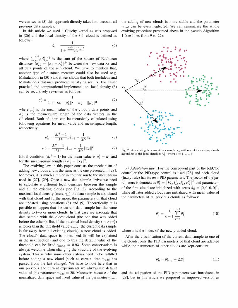
The evolving law in this paper consists the mechanism ofadding new clouds and is the same as the one presented in [28].Moreover, it is much simpler in comparison to the mechanismused in [27], [29]. Once a new data sample arrive we needto calculate c different local densities between the sampleand all the existing clouds (see Fig. 2). According to themaximal local density (maxi γ

ik) the data sample is associated

with that cloud and furthermore, the parameters of that cloudare updated using equations (8) and (9). Theoretically, it ispossible to happen that the current data sample has the samedensity to two or more clouds. In that case we associate thatdata sample with the oldest cloud (the one that was addedbefore the others). But, if the maximal local density (maxi γ

ik)

is lower than the threshold value γmax (the current data sampleis far away from all existing clouds), a new cloud is added.The cloud’s data space is normalized (it will be explainedin the next section) and due to this the default value of thethreshold can be fixed γmax = 0.93. Some conservatism isalways welcome when changing the structure of the evolvingsystem. This is why some other criteria need to be fulfilledbefore adding a new cloud (such as certain time nadd haspassed from the last change). We have to note here that inour previous and current experiments we always use defaultvalue of this parameter nadd = 20. Moreover, because of thenormalized data space and fixed value of the parameter γmax

the adding of new clouds is more stable and the parameternadd can be even neglected. We can summarize the wholeevolving procedure presented above in the pseudo Algorithm1 (see lines from 9 to 22).

xk

γ1k

γ2k

γck

Fig. 2. Associating the current data sample xk with one of the existing cloudsaccording to the local densities γik , where i = 1, . . . , c

3) Adaptation law: For the consequent part of the RECCocontroller the PID-type control is used [28] and each cloud(fuzzy rule) has its own PID parameters. The vector of the pa-rameters is denoted as θik =

[P ik, I

ik, D

ik, R

ik

]Tand parameters

of the first cloud are initialized with zeros θ10 = [0, 0, 0, 0]

T ,while all later added clouds are initialized with mean value ofthe parameters of all previous clouds as follows:

θc0 =1

c− 1

c−1∑j=1

θjk (10)

where c is the index of the newly added cloud.

After the classification of the current data sample to one ofthe clouds, only the PID parameters of that cloud are adaptedwhile the parameters of other clouds are kept constant:

θik = θik−1 + ∆θik (11)

and the adaptation of the PID parameters was introduced in[28], but in this article we proposed an improved version as

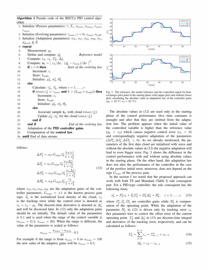
Algorithm 1 Pseudo code of the RECCo PID control algo-rithm

1: Initialize (Process parameters): τ , Ts, umin, umax, rmin,rmax.

2: Initialize (Evolving parameters): γmax, c = 0, cmax, nadd.3: Initialize (Adaptation parameters): αP , αI , αD, αR, σL,ddead, θ, θ.

4: repeat5: Measurement: yk.6: Define and compute: yrk . Reference model7: Compute: ek, εk, Σεk, ∆ε

k.8: Compute: xk = [ εk/∆ε, (yrk − rmin)/∆r ]

T .9: if c = 0 then . Start of the evolving law

10: Increment: c,11: Store: kadd,12: Initialize: µ1

0, σ10 , θ1

0 .13: else14: Calculate: γik, λik, where i = 1, . . . , c15: if (maxiγik < γmax and k > (kadd + nadd)) then16: Increment: c,17: Store: kadd,18: Initialize: µc0, σc0, θc0.19: else20: Associate sample xk with cloud (maxiγik)21: Update µik, σik for the cloud (maxiγik)22: end if23: end if . End of the evolving law24: Adaptation of the PID controller gains.25: Computation of the control law.26: until End of data stream.

follows:

∆P ik = αP Gsignλik

|ekεk|1 + r2

k

∆Iik = αI Gsignλik

|ek∆εk|

1 + r2k

∆Dik = αD Gsignλ

ik

|ek∆εk|

1 + r2k

∆Rik = αRGsignλik

εk1 + r2

k

(12)

where αP , αI , αD, αR are the adaptation gains of the con-troller parameters, Gsign = ±1 is the known process gainsign, λik is the normalized local density of the cloud, εkis the tracking error while the control error is denoted asek = rk − yk. The discrete-time derivative is denoted as ∆ε

k

and will be discussed later. In (12) only the adaptation gainsshould be set initially. The default value of the parametersis 0.1 and is used when the range of the control variable is(umin = 0/4, umax = 20). When the range is different, thevalue of the parameters is scaled as follows:

αnew =umax − umin

20· 0.1

For example if the range is from umin = 0 to umax = 100the new value of the adaptive gains will be αnew = 0.5.

0 10 20 30 40 50 6020

25

30

35

40

45

50

55

t [min]

[◦C]

rkyrkyk

0 10 20 30 40 50 6020

25

30

35

40

45

50

55

t [min]

[◦C]

rkyrkyk

Fig. 3. The reference, the model reference and the controlled signal for heat-exchanger pilot plant in the starting phase with (upper plot) and without (lowerplot) calculating the absolute value in adaptation law of the controller gains(y0 = 32 ◦C, r0 = 25 ◦C).

The absolute values in (12) are used only in the startingphase of the control performance (five time constants isenough) and after that they are omitted from the adapta-tion law. The problem appears when the initial value ofthe controlled variable is higher than the reference value(y0 > r0) which causes negative control error (ek < 0)and correspondingly negative adaptation of the parameters(∆P ik,∆I

ik,∆D

ik < 0). As we already mentioned, the pa-

rameters of the first data cloud are initialized with zeros andwithout the absolute values in (12) the negative adaptation willlead to even bigger error. Fig. 3 shows the difference in thecontrol performance with and without using absolute valuesin the starting phase. On the other hand, this adaptation lawdoes not alter the performance of the controller in the caseof the positive initial error, moreover, does not depend on thesign Gsign of the process gain.

In the section I we noted that the proposed approach canwork with both TS and Mamdani (Table I) rule consequentpart. For a PID-type controller, the rule consequent has thefollowing form:

uik = P ikεk + IikΣεk +Di

k∆εk +Rik, i = 1, . . . , c (13)

where P ik, Iik, D

ik are controller gains while Rik is compen-

sation of the operating point. While the adaptation of theparameter Rik in (12) is driven only by tracking error εkthis parameter tries to correct the offset error of the currentoperating point. Σε

k and ∆εk in (13) are discrete-time integral

and derivative of the tracking error, respectively, and can becalculated as follows:

Σεk =

k−1∑κ=0

εκ = Σεk−1 + εk−1 (14)

∆εk = εk − εk−1 (15)

Finally, for the defuzzification the weighted average is used(but not limited to this form) and furthermore, the controlvariable becomes:

uk = umin +

c∑i=1

λikui = umin +

c∑i=1

γikui

c∑i=1

γik

(16)

where ui denotes the i-th (partial) rule consequent andnormalized relative density (2) is used. From the practicalimplementation point of view we add umin in this equation (incomparison with the one proposed in [27], [28]) and representsthe minimal input value of the real actuator which in our caseis umin = 4 mA.

C. The instability protection mechanism

This subsection is devoted to the modifications of the adap-tation law (11) that improve the robustness of the closed-loopsystem. Supervised adaptation of any controller can improve,theoretically and practically, the performance and robustnessof the controller. In order to minimize the negative influenceof parasitics, disturbances in the system and to eliminate thepure integral action of the adaptive law, we introduce severalmechanisms to improve the RECCo control algorithm.

When dealing with adaptive controllers and parameteradaptation we need to be aware of the potential instabilityproblems caused by the parameter drift [36]. Due to this, tomake RECCo controller more robust, several techniques werealready applied in [27] and [28]. In this paper we will use thefollowing techniques:

1) Dead zone in the adaptation law: To improve the robust-ness under the unknown bounded disturbances and modelingerrors, the RECCo controller includes a dead-zone in adapta-tion law. The general idea behind the dead-zone mechanism,in case of bounded disturbances, is to turn off the adaptationalgorithm when the absolute value of the tracking error issmaller than a certain threshold [37]:

∆θik =

{∆θik |εk| ≥ ddead0 |εk| < ddead

i = 1, . . . , c (17)

The parameter ddead should be chosen slightly larger thanthe process noise to improve the effectiveness of the adaptivelaw. A larger threshold implies a shorter adaptation period andlarger tracking error, while smaller value can lead to parameterdrift.

2) Parameter projection: Parameter projection mechanismis used to guarantee that the estimation of the parameters willstay within finite known region [38]. In the case of the positiveplant gain all the parameters should be bounded by 0 frombellow while upper bound may or may not be provided. Theadaptive law in (11) is generalized as follows:

θik =

θik−1 + ∆θik θ ≤ θik−1 + ∆θik ≤ θθ θik−1 + ∆θik < θ

θ θik−1 + ∆θik > θ

i = 1, . . . , c

(18)

In our case we chose θ = 0 and θ =∞ for the controller gainsPk, Ik, and Dk, while for the compensation of the operatingpoint Rk the lower bound was θ = −∞. If we have some apriori knowledge where the true parameters θ∗ are located inRn we can define upper and lower bound for the elements of θ.The benefit of such information may speed up the convergenceof finding optimal parameters.

3) Leakage in the adaptation law: The use of leakage inthe adaptation law is a very known approach for improvementof robustness of adaptive control. Already exist different typesof leakage, for example σ-modification [39], e1-modification[40], switching σ-modification [41] etc.

Including the leakage in the adaptation law results in:

θik = (1− σL)θik−1 + ∆θik i = 1, . . . , c (19)

where σL defines the extent of the leakage.4) Interruption of adaptation: In the RECCo algorithm we

first calculate the adaptation of the PID parameters (∆θik) andthen the control variable uk. In some cases this two stepscan be in conflict, which means that the adaptation causescontrol signal which is outside the limits [umin, umax]. In suchcase the adaptive law should be interrupted in the followingmanner:

∆θik =

{∆θik umin ≤ uk ≤ umax0 otherwise

i = 1, . . . , c (20)

yrk−rmin

∆r

1

0 εk∆ε

−0.5 0.5

xk

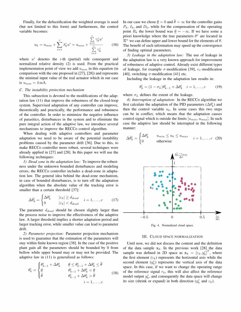
Fig. 4. Normalized cloud space.

III. CLOUD SPACE NORMALIZATION

Until now, we did not discuss the content and the definitionof the data sample xk. In the previous work [28] the datasample was defined in 2D space as xk = [εk, y

rk]T , where

the first element (εk) represents the horizontal axis while thesecond element (yrk) represents the vertical axis of the dataspace. In this case, if we want to change the operating rangeof the reference signal rk, this will also affect the referencemodel output yrk, and consequently the data space will changeits size (shrink or expand) in both direction (yrk and εk).

Our idea is to define a constant data space (see Fig. 4),where majority of the data will appear, regardless of the rangeof the reference signal. Even if we want to control a differentprocess, the same data normalization can be used with thesame constant data space. As a consequence, the evolvingparameter γmax can be fixed. We propose a normalized dataspace as follows:

x =[

εk∆ε ,

yrk−rmin

∆r

]T(21)

where ∆r = rmax − rmin and ∆ε = ∆r2 . In this case the

operator (user) needs to choose, according to the process re-quirements, only the operating range of the plant [rmin, rmax].After that, several step changes of the reference signal rk areconstructed to cover the whole range of the process (e.g. seeupper plot in Fig. 12).

IV. EXPERIMENTAL RESULTS OF A HEAT-EXCHANGERPILOT PLANT

A. Comparison between RECCo and classical PID controllers

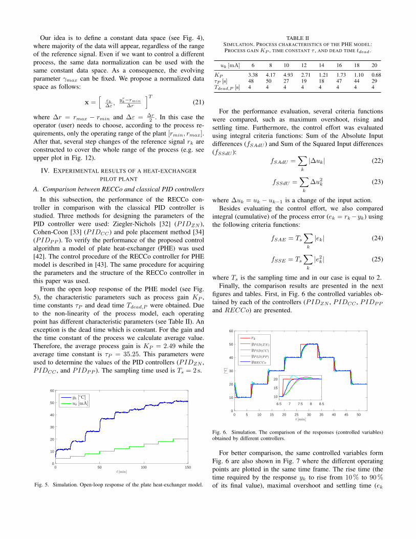
In this subsection, the performance of the RECCo con-troller in comparison with the classical PID controller isstudied. Three methods for designing the parameters of thePID controller were used: Ziegler-Nichols [32] (PIDZN ),Cohen-Coon [33] (PIDCC) and pole placement method [34](PIDPP ). To verify the performance of the proposed controlalgorithm a model of plate heat-exchanger (PHE) was used[42]. The control procedure of the RECCo controller for PHEmodel is described in [43]. The same procedure for acquiringthe parameters and the structure of the RECCo controller inthis paper was used.

From the open loop response of the PHE model (see Fig.5), the characteristic parameters such as process gain KP ,time constants τP and dead time Tdead,P were obtained. Dueto the non-linearity of the process model, each operatingpoint has different characteristic parameters (see Table II). Anexception is the dead time which is constant. For the gain andthe time constant of the process we calculate average value.Therefore, the average process gain is KP = 2.49 while theaverage time constant is τP = 35.25. This parameters wereused to determine the values of the PID controllers (PIDZN ,PIDCC , and PIDPP ). The sampling time used is Ts = 2 s.

0 50 100 150t [min]

0

10

20

30

40

50

60

yk [◦C]

uk [mA]

Fig. 5. Simulation. Open-loop response of the plate heat-exchanger model.

TABLE IISIMULATION. PROCESS CHARACTERISTICS OF THE PHE MODEL:PROCESS GAIN KP , TIME CONSTANT τ , AND DEAD TIME tdead .

uk [mA] 6 8 10 12 14 16 18 20

KP 3.38 4.17 4.93 2.71 1.21 1.73 1.10 0.68τP [s] 48 50 27 19 18 47 44 29Tdead,P [s] 4 4 4 4 4 4 4 4

For the performance evaluation, several criteria functionswere compared, such as maximum overshoot, rising andsettling time. Furthermore, the control effort was evaluatedusing integral criteria functions: Sum of the Absolute Inputdifferences (fSAdU ) and Sum of the Squared Input differences(fSSdU ):

fSAdU =∑k

|∆uk| (22)

fSSdU =∑k

∆u2k (23)

where ∆uk = uk − uk−1 is a change of the input action.Besides evaluating the control effort, we also compared

integral (cumulative) of the process error (ek = rk−yk) usingthe following criteria functions:

fSAE = Ts∑k

|ek| (24)

fSSE = Ts∑k

|e2k| (25)

where Ts is the sampling time and in our case is equal to 2.Finally, the comparison results are presented in the next

figures and tables. First, in Fig. 6 the controlled variables ob-tained by each of the controllers (PIDZN , PIDCC , PIDPP

and RECCo) are presented.

0 5 10 15 20 25 30 35 40 45 50t [min]

0

10

20

30

40

50

60

[◦C]

rkyPID(ZN )

yPID(CC)

yPID(PP )

yRECCo

6.5 7 7.5 8 8.5

10

15

20

Fig. 6. Simulation. The comparison of the responses (controlled variables)obtained by different controllers.

For better comparison, the same controlled variables formFig. 6 are also shown in Fig. 7 where the different operatingpoints are plotted in the same time frame. The rise time (thetime required by the response yk to rise from 10 % to 90 %of its final value), maximal overshoot and settling time (ek

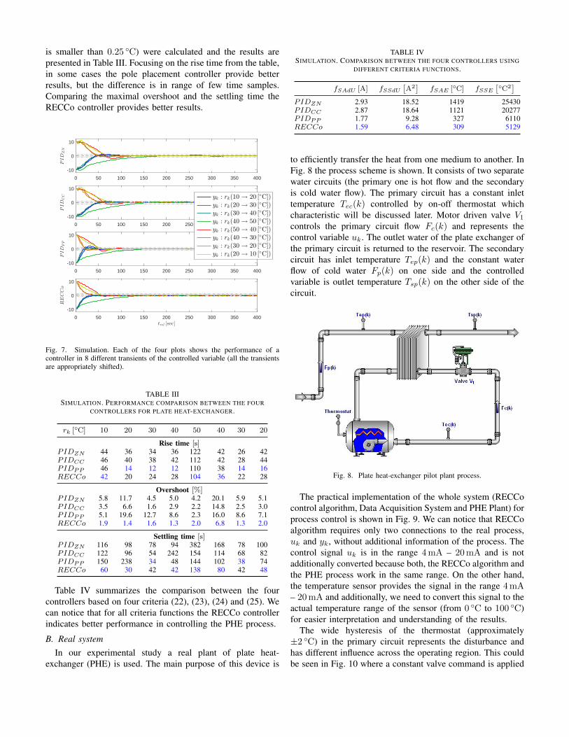
is smaller than 0.25 ◦C) were calculated and the results arepresented in Table III. Focusing on the rise time from the table,in some cases the pole placement controller provide betterresults, but the difference is in range of few time samples.Comparing the maximal overshoot and the settling time theRECCo controller provides better results.

0 50 100 150 200 250 300 350 400

-10

0

10

PID

ZN

0 50 100 150 200 250 300 350 400

-10

0

10

PID

CC

0 50 100 150 200 250 300 350 400

-10

0

10

PID

PP

0 50 100 150 200 250 300 350 400trel [sec]

-10

0

10

RECCo

yk : rk(10 → 20 [◦C])

yk : rk(20 → 30 [◦C])

yk : rk(30 → 40 [◦C])

yk : rk(40 → 50 [◦C])

yk : rk(50 → 40 [◦C])

yk : rk(40 → 30 [◦C])

yk : rk(30 → 20 [◦C])

yk : rk(20 → 10 [◦C])

Fig. 7. Simulation. Each of the four plots shows the performance of acontroller in 8 different transients of the controlled variable (all the transientsare appropriately shifted).

TABLE IIISIMULATION. PERFORMANCE COMPARISON BETWEEN THE FOUR

CONTROLLERS FOR PLATE HEAT-EXCHANGER.

rk [◦C] 10 20 30 40 50 40 30 20

Rise time [s]PIDZN 44 36 34 36 122 42 26 42PIDCC 46 40 38 42 112 42 28 44PIDPP 46 14 12 12 110 38 14 16RECCo 42 20 24 28 104 36 22 28

Overshoot [%]PIDZN 5.8 11.7 4.5 5.0 4.2 20.1 5.9 5.1PIDCC 3.5 6.6 1.6 2.9 2.2 14.8 2.5 3.0PIDPP 5.1 19.6 12.7 8.6 2.3 16.0 8.6 7.1RECCo 1.9 1.4 1.6 1.3 2.0 6.8 1.3 2.0

Settling time [s]PIDZN 116 98 78 94 382 168 78 100PIDCC 122 96 54 242 154 114 68 82PIDPP 150 238 34 48 144 102 38 74RECCo 60 30 42 42 138 80 42 48

Table IV summarizes the comparison between the fourcontrollers based on four criteria (22), (23), (24) and (25). Wecan notice that for all criteria functions the RECCo controllerindicates better performance in controlling the PHE process.

B. Real systemIn our experimental study a real plant of plate heat-

exchanger (PHE) is used. The main purpose of this device is

TABLE IVSIMULATION. COMPARISON BETWEEN THE FOUR CONTROLLERS USING

DIFFERENT CRITERIA FUNCTIONS.

fSAdU [A] fSSdU[A2]

fSAE [◦C] fSSE[◦C2

]PIDZN 2.93 18.52 1419 25430PIDCC 2.87 18.64 1121 20277PIDPP 1.77 9.28 327 6110RECCo 1.59 6.48 309 5129

to efficiently transfer the heat from one medium to another. InFig. 8 the process scheme is shown. It consists of two separatewater circuits (the primary one is hot flow and the secondaryis cold water flow). The primary circuit has a constant inlettemperature Tec(k) controlled by on-off thermostat whichcharacteristic will be discussed later. Motor driven valve V1

controls the primary circuit flow Fc(k) and represents thecontrol variable uk. The outlet water of the plate exchanger ofthe primary circuit is returned to the reservoir. The secondarycircuit has inlet temperature Tep(k) and the constant waterflow of cold water Fp(k) on one side and the controlledvariable is outlet temperature Tsp(k) on the other side of thecircuit.

Fig. 8. Plate heat-exchanger pilot plant process.

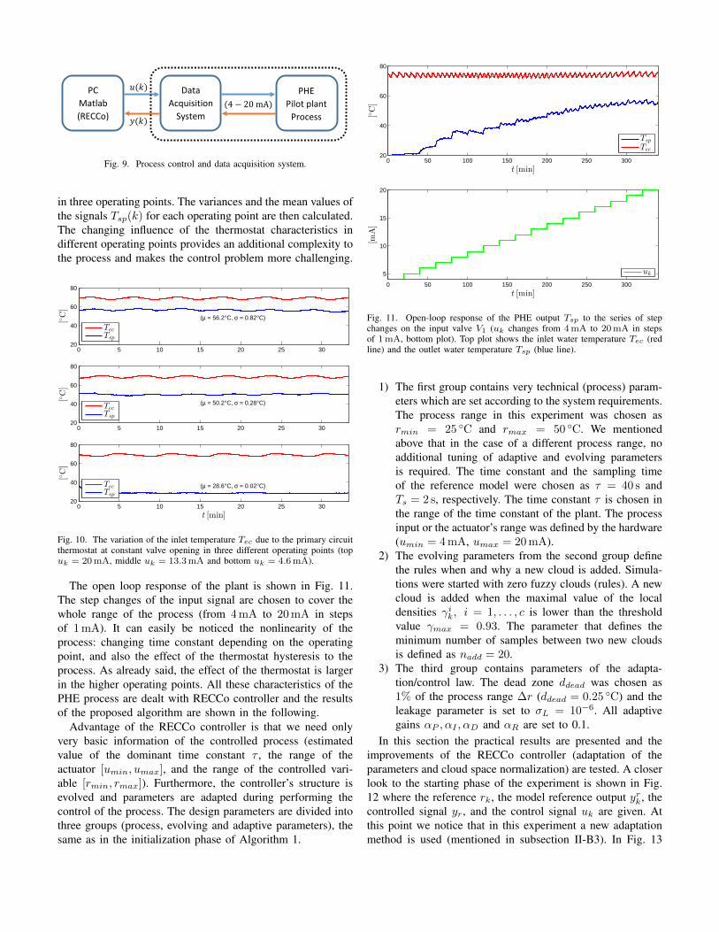
The practical implementation of the whole system (RECCocontrol algorithm, Data Acquisition System and PHE Plant) forprocess control is shown in Fig. 9. We can notice that RECCoalgorithm requires only two connections to the real process,uk and yk, without additional information of the process. Thecontrol signal uk is in the range 4 mA – 20 mA and is notadditionally converted because both, the RECCo algorithm andthe PHE process work in the same range. On the other hand,the temperature sensor provides the signal in the range 4 mA– 20 mA and additionally, we need to convert this signal to theactual temperature range of the sensor (from 0 ◦C to 100 ◦C)for easier interpretation and understanding of the results.

The wide hysteresis of the thermostat (approximately±2 ◦C) in the primary circuit represents the disturbance andhas different influence across the operating region. This couldbe seen in Fig. 10 where a constant valve command is applied

PC

Matlab (RECCo)

Data Acquisition

System

PHE Pilot plant

Process

𝑢𝑢(𝑘𝑘)

𝑦𝑦(𝑘𝑘)

(4 − 20 mA)

Fig. 9. Process control and data acquisition system.

in three operating points. The variances and the mean values ofthe signals Tsp(k) for each operating point are then calculated.The changing influence of the thermostat characteristics indifferent operating points provides an additional complexity tothe process and makes the control problem more challenging.

0 5 10 15 20 25 3020

40

60

80

(µ = 56.2°C, σ = 0.82°C)[◦C]

Tec

Tsp

0 5 10 15 20 25 3020

40

60

80

(µ = 50.2°C, σ = 0.28°C)[◦C]

Tec

Tsp

0 5 10 15 20 25 3020

40

60

80

(µ = 28.6°C, σ = 0.02°C)

t [min]

[◦C]

Tec

Tsp

Fig. 10. The variation of the inlet temperature Tec due to the primary circuitthermostat at constant valve opening in three different operating points (topuk = 20mA, middle uk = 13.3mA and bottom uk = 4.6mA).

The open loop response of the plant is shown in Fig. 11.The step changes of the input signal are chosen to cover thewhole range of the process (from 4 mA to 20 mA in stepsof 1 mA). It can easily be noticed the nonlinearity of theprocess: changing time constant depending on the operatingpoint, and also the effect of the thermostat hysteresis to theprocess. As already said, the effect of the thermostat is largerin the higher operating points. All these characteristics of thePHE process are dealt with RECCo controller and the resultsof the proposed algorithm are shown in the following.

Advantage of the RECCo controller is that we need onlyvery basic information of the controlled process (estimatedvalue of the dominant time constant τ , the range of theactuator [umin, umax], and the range of the controlled vari-able [rmin, rmax]). Furthermore, the controller’s structure isevolved and parameters are adapted during performing thecontrol of the process. The design parameters are divided intothree groups (process, evolving and adaptive parameters), thesame as in the initialization phase of Algorithm 1.

0 50 100 150 200 250 30020

40

60

80

t [min]

[◦C]

Tsp

Tec

0 50 100 150 200 250 300

5

10

15

20

t [min]

[mA]

uk

Fig. 11. Open-loop response of the PHE output Tsp to the series of stepchanges on the input valve V1 (uk changes from 4mA to 20mA in stepsof 1mA, bottom plot). Top plot shows the inlet water temperature Tec (redline) and the outlet water temperature Tsp (blue line).

1) The first group contains very technical (process) param-eters which are set according to the system requirements.The process range in this experiment was chosen asrmin = 25 ◦C and rmax = 50 ◦C. We mentionedabove that in the case of a different process range, noadditional tuning of adaptive and evolving parametersis required. The time constant and the sampling timeof the reference model were chosen as τ = 40 s andTs = 2 s, respectively. The time constant τ is chosen inthe range of the time constant of the plant. The processinput or the actuator’s range was defined by the hardware(umin = 4 mA, umax = 20 mA).

2) The evolving parameters from the second group definethe rules when and why a new cloud is added. Simula-tions were started with zero fuzzy clouds (rules). A newcloud is added when the maximal value of the localdensities γik, i = 1, . . . , c is lower than the thresholdvalue γmax = 0.93. The parameter that defines theminimum number of samples between two new cloudsis defined as nadd = 20.

3) The third group contains parameters of the adapta-tion/control law. The dead zone ddead was chosen as1% of the process range ∆r (ddead = 0.25 ◦C) and theleakage parameter is set to σL = 10−6. All adaptivegains αP , αI , αD and αR are set to 0.1.

In this section the practical results are presented and theimprovements of the RECCo controller (adaptation of theparameters and cloud space normalization) are tested. A closerlook to the starting phase of the experiment is shown in Fig.12 where the reference rk, the model reference output yrk, thecontrolled signal yr, and the control signal uk are given. Atthis point we notice that in this experiment a new adaptationmethod is used (mentioned in subsection II-B3). In Fig. 13

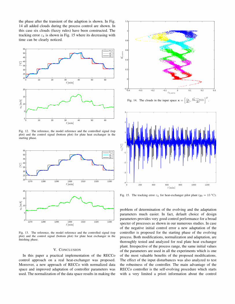
the phase after the transient of the adaption is shown. In Fig.14 all added clouds during the process control are shown. Inthis case six clouds (fuzzy rules) have been constructed. Thetracking error εk is shown in Fig. 15 where its decreasing withtime can be clearly noticed.

0 10 20 30 40 50 6020

25

30

35

40

45

50

55

t [min]

[◦C]

rkyrkyk

0 10 20 30 40 50 600

5

10

15

20

t [min]

uk[m

A]

Fig. 12. The reference, the model reference and the controlled signal (topplot) and the control signal (bottom plot) for plate heat exchanger in thestarting phase.

1270 1280 1290 1300 1310 1320 133020

25

30

35

40

45

50

55

t [min]

[◦C]

rkyrkyk

1270 1280 1290 1300 1310 1320 13300

5

10

15

20

t [min]

uk[m

A]

Fig. 13. The reference, the model reference and the controlled signal (topplot) and the control signal (bottom plot) for plate heat exchanger in thefinishing phase.

V. CONCLUSION

In this paper a practical implementation of the RECCocontrol approach on a real heat-exchanger was proposed.Moreover, a new approach of RECCo with normalized dataspace and improved adaptation of controller parameters wasused. The normalization of the data space results in making the

−0.4 −0.3 −0.2 −0.1 0 0.1 0.2 0.3−0.2

0

0.2

0.4

0.6

0.8

1

1.2

εk,norm

yr k,norm

Fig. 14. The clouds in the input space x =[εk∆ε,yrk−rmin

∆r

]T.

0 200 400 600 800 1000 1200

t [min]

-4

-3

-2

-1

0

1

2

3

εk[◦C]

Fig. 15. The tracking error εk for heat-exchanger pilot plant (y0 = 15 ◦C).

problem of determination of the evolving and the adaptationparameters much easier. In fact, default choice of designparameters provides very good control performance for a broadspecter of processes as shown in our numerous studies. In caseof the negative initial control error a new adaptation of thecontroller is proposed for the starting phase of the evolvingprocess. Both modifications, normalization and adaptation, arethoroughly tested and analyzed for real plate heat exchangerplant. Irrespective of the process range, the same initial valuesof the parameters are used in all the experiments which is oneof the most valuable benefits of the proposed modifications.The effect of the input disturbances was also analyzed to testthe robustness of the controller. The main advantage of theRECCo controller is the self-evolving procedure which startswith a very limited a priori information about the control

process (only the range of the control and controlled variableare needed and a rough estimate of the dominant time constantof the controlled process). This approach effectively deals withnonlinear processes.

REFERENCES

[1] W.-D. Chang, R.-C. Hwang, and J.-G. Hsieh, “A self-tuning pid controlfor a class of nonlinear systems based on the lyapunov approach,”Journal of Process Control, vol. 12, pp. 233–242, 2002.

[2] Y. Kansha, L. Jia, and M.-S. Chiu, “Self-tuning PID controllers based onthe Lyapunov approach,” Chemical Engineering Science, vol. 63, no. 10,pp. 2732 – 2740, 2008.

[3] C. Riverol and V. Napolitano, “Use of Neural Networks as a TuningMethod for an Adaptive PID: Application in a Heat Exchanger,” Chem-ical Engineering Research and Design, vol. 78, no. 8, pp. 1115 – 1119,2000.

[4] A. Altinten, S. Erdogan, F. Alioglu, H. Hapoglu, and M. Alpbaz, “Appli-cation of adaptive PID control with genetic algorithm to a polymerizationreactor,” Chemical Engineering Communications, vol. 191, no. 9, pp.1158–1172, 2004.

[5] A. Moharam, M. A. El-Hosseini, and H. A. Ali, “Design of optimalPID controller using hybrid differential evolution and particle swarmoptimization with an aging leader and challengers,” Applied Soft Com-puting, vol. 38, pp. 727 – 737, 2016.

[6] I. Podlubny, “Fractional-order systems and PIλDµ−controllers,” IEEETransactions on Automatic Control, vol. 44, no. 1, pp. 208–214, Jan1999.

[7] J. A. Tenreiro Machado, “Optimal tuning of fractional controllers usinggenetic algorithms,” Nonlinear Dynamics, vol. 62, no. 1, pp. 447–452,2010.

[8] J. T. Machado, A. M. Galhano, A. M. Oliveira, and J. K. Tar, “Optimalapproximation of fractional derivatives through discrete-time fractionsusing genetic algorithms,” Communications in Nonlinear Science andNumerical Simulation, vol. 15, no. 3, pp. 482 – 490, 2010.

[9] Y. Mousavi and A. Alfi, “A memetic algorithm applied to trajectorycontrol by tuning of fractional order proportional-integral-derivativecontrollers,” Applied Soft Computing, vol. 36, pp. 599 – 617, 2015.

[10] Y. Bai, H. Zhuang, and Z. S. Roth, “Fuzzy logic control to suppressnoises and coupling effects in a laser tracking system,” IEEE Transac-tions on Control Systems Technology, vol. 13, no. 1, pp. 113–121, Jan2005.

[11] I. Baturone, F. Moreno-Velo, S. Sanchez-Solano, and A. Ollero, “Auto-matic design of fuzzy controllers for car-like autonomous robots,” IEEETransactions on Fuzzy Systems, vol. 12, no. 4, pp. 447–465, Aug 2004.

[12] P. Bonissone, V. Badami, K. Chiang, P. Khedkar, K. Marcelle, andM. Schutten, “Induial applications of fuzzy logic at general electric,”Proceedings of the IEEE, vol. 83, no. 3, pp. 450–465, Mar 1995.

[13] Z. Bingul, G. Cook, A. Strauss, and K. Rashid, “Application of fuzzylogic to spatial thermal control in fusion welding,” in Industry Applica-tions Conference, 1999. Thirty-Fourth IAS Annual Meeting. ConferenceRecord of the 1999 IEEE, vol. 1, 1999, pp. 627–634 vol.1.

[14] R. Boukezzoula, S. Galichet, and L. Foulloy, “Observer-based fuzzyadaptive control for a class of nonlinear systems: real-time imple-mentation for a robot wrist,” IEEE Transactions on Control SystemsTechnology, vol. 12, no. 3, pp. 340–351, May 2004.

[15] W.-J. Chang and P.-H. Chen, Stabilization for truck-trailer mobile robotsystem via discrete LPV T-S fuzzy models. Berlin, Heidelberg: Springer-Verlag, 2013, vol. 193, ch. Intelligent Autonomous Systems 12, pp. 209–217.

[16] L. E. Ramos-Velasco, O. A. Domnguez-Ramrez, and V. Parra-Vega,“Wavenet fuzzy PID controller for nonlinear MIMO systems: Exper-imental validation on a high-end haptic robotic interface,” Applied SoftComputing, vol. 40, pp. 199 – 205, 2016.

[17] S. Fidanova and P. Pop, “An improved hybrid ant-local search algorithmfor the partition graph coloring problem,” Journal of Computational andApplied Mathematics, vol. 293, pp. 55 – 61, 2016.

[18] L. A. Zadeh, “Outline of a new approach to the analysis of complexsystems and decision processes,” IEEE Transactions on Systems, Manand Cybernetics, vol. SMC-3, no. 1, pp. 28–44, Jan 1973.

[19] E. Mamdani, “Application of fuzzy algorithms for control of simpledynamic plant,” Proceedings of the Institution of Electrical Engineers,vol. 121, no. 12, pp. 1585–1588, December 1974.

[20] T. Takagi and M. Sugeno, “Fuzzy identification of systems and itsapplications to modeling and control,” IEEE Transactions on Systems,Man and Cybernetics, vol. SMC-15, no. 1, pp. 116–132, Jan 1985.

[21] G. Feng, “A survey on analysis and design of model-based fuzzy controlsystems,” IEEE Transactions on Fuzzy Systems, vol. 14, no. 5, pp. 676–697, Oct 2006.

[22] R. E. Precup, L. T. Dioanca, E. M. Petriu, M. B. Rdac, S. Preitl, andC. A. Drago, “Tensor product-based real-time control of the liquid levelsin a three tank system,” in 2010 IEEE/ASME International Conferenceon Advanced Intelligent Mechatronics, July 2010, pp. 768–773.

[23] P. Baranyi, P. Korondi, and K. Tanaka, “Parallel Distributed Compensa-tion Based Stabilization of A 3DOF RC Helicopter: A Tensor ProductTransformation Based Approach,” Journal of Advanced ComputationalIntelligence and Intelligent Informatics, vol. 13, pp. 25–34, 2009.

[24] P. Grf, P. Baranyi, and P. Korondi, “Determination of the stability pa-rameter space of a two dimensional aeroelastic system, a tp model-basedapproach,” in 2010 IEEE 14th International Conference on IntelligentEngineering Systems, May 2010, pp. 265–270.

[25] R. E. Precup, C. A. Dragos, S. Preitl, M. B. Radac, and E. M.Petriu, “Novel tensor product models for automatic transmission systemcontrol,” IEEE Systems Journal, vol. 6, no. 3, pp. 488–498, Sept 2012.

[26] P. Angelov and R. Yager, “Simplified fuzzy rule-based systems usingnon-parametric antecedents and relative data density,” in 2011 IEEEWorkshop on Evolving and Adaptive Intelligent Systems (EAIS), April2011, pp. 62–69.

[27] P. Angelov, I. Skrjanc, and S. Blazic, “Robust evolving cloud-basedcontroller for a hydraulic plant,” in 2013 IEEE Conference on Evolvingand Adaptive Intelligent Systems (EAIS), April 2013, pp. 1–8.

[28] I. Skrjanc, S. Blazic, and P. Angelov, “Robust evolving cloud-based PIDcontrol adjusted by gradient learning method,” in 2014 IEEE Conferenceon Evolving and Adaptive Intelligent Systems (EAIS), June 2014, pp. 1–8.

[29] B. Costa, I. Skrjanc, S. Blazic, and P. Angelov, “A practical implementa-tion of self-evolving cloud-based control of a pilot plant,” in 2013 IEEEInternational Conference on Cybernetics (CYBCONF), June 2013, pp.7–12.

[30] S. Blazic, D. Dovzan, and I. Skrjanc, “Cloud-based identification ofan evolving system with supervisory mechanisms,” in 2014 IEEEInternational Symposium on Intelligent Control (ISIC), Oct 2014, pp.1906–1911.

[31] G. Andonovski, S. Blazic, P. Angelov, and I. Skrjanc, “Analysis ofadaptation law of the robust evolving cloud-based controller,” in 2015IEEE International Conference on Evolving and Adaptive IntelligentSystems (EAIS), Dec 2015, pp. 1–7.

[32] N. N. J. Ziegler, “Optimum settings for automatic controllers,” Trans-actions of ASME64, 1942.

[33] G. Cohen and G. Coon, “Theoretical consideration of retarded control,”Transactions of ASME, vol. 75, pp. 827–834, 1953.

[34] K. J. AAstrom and T. Hagglund, PID Controllers: Theory, Design, andTuning, 2nd ed. Instrument Society of America, Research TrianglePark, NC, 1995.

[35] H. Kaufman, I. Barkana, and K. Sobel, Direct Adaptive Control Algo-rithms. New York: Springer-Verlag, 1998.

[36] C. Rohrs, L. Valavani, M. Athans, and G. Stein, “Robustness ofcontinuous-time adaptive control algorithms in the presence of unmod-eled dynamics,” IEEE Transactions on Automatic Control, vol. 30, no. 9,pp. 881–889, Sep 1985.

[37] B. Peterson and K. Narendra, “Bounded error adaptive control,” IEEETransactions on Automatic Control, vol. 27, no. 6, pp. 1161–1168, Dec1982.

[38] G. Kreisselmeier and K. Narendra, “Stable model reference adaptivecontrol in the presence of bounded disturbances,” IEEE Transactions onAutomatic Control, vol. 27, no. 6, pp. 1169–1175, Dec 1982.

[39] P. Ioannou and P. Kokotovic, “Instability analysis and improvement ofrobustness of adaptive control,” Automatica, vol. 20, no. 5, pp. 583 –594, 1984.

[40] K. Narendra and A. Annaswamy, “A new adaptive law for robust adap-tation without persistent excitation,” in American Control Conference,June 1986, pp. 1067–1072.

[41] P. Ioannou and K. S. Tsakalis, “A robust direct adaptive controller,” IEEETransactions on Automatic Control, vol. 31, no. 11, pp. 1033–1043, Nov1986.

[42] I. Skrjanc and D. Matko, “Predictive functional control based on fuzzymodel for heat-exchanger pilot plant,” IEEE Transactions on FuzzySystems, vol. 8, no. 6, pp. 705–712, Dec 2000.

[43] G. Andonovski, S. Blazic, P. Angelov, and I. Skrjanc, “Robust evolvingcloud-based controller in normalized data space for heat-exchangerplant,” in 2015 IEEE International Conference on Fuzzy Systems (FUZZ-IEEE), Aug 2015, pp. 1–7.