A Practical Guide to Computer Simulations

arX

iv:c

ond-

mat

/011

1531

v1 2

8 N

ov 2

001

A practical guide to computer simulations ∗

Alexander K. Hartmann

University of Gottingen, Germany

[email protected]

Heiko Rieger

University of Saarbrucken, Germany

[email protected]

February 1, 2008

Abstract

Here practical aspects of conducting research via computer simulationsare discussed. The following issues are addressed: software engineering,object-oriented software development, programming style, macros, make

files, scripts, libraries, random numbers, testing, debugging, data plot-ting, curve fitting, finite-size scaling, information retrieval, and preparingpresentations.

Because of the limited space, usually only short introductions to thespecific areas are given and references to more extensive literature arecited. All examples of code are in C/C++.

Contents

1 Software Engineering 3

2 Object-oriented Software Development 10

3 Programming Style 16

4 Programming Tools 204.1 Using Macros . . . . . . . . . . . . . . . . . . . . . . . . . . . . . 204.2 Make Files . . . . . . . . . . . . . . . . . . . . . . . . . . . . . . 244.3 Scripts . . . . . . . . . . . . . . . . . . . . . . . . . . . . . . . . . 28

∗Taken from the book: A.K. Hartmann and H. Rieger, Optimization Algorithms in Physics,(Wiley-VCH, Berlin, Weinheim 2001), ISBN 3-527-40307-8, with permission of Wiley-VCH,see http://www.wiley.com. This document may be distributed freely in electronic and non-electronic form, provided that no changes are performed to it.

1

http://arXiv.org/abs/cond-mat/0111531v1

5 Libraries 295.1 Numerical Recipes . . . . . . . . . . . . . . . . . . . . . . . . . . 295.2 LEDA . . . . . . . . . . . . . . . . . . . . . . . . . . . . . . . . . 315.3 Creating your own Libraries . . . . . . . . . . . . . . . . . . . . . 33

6 Random Numbers 346.1 Generating Random Numbers . . . . . . . . . . . . . . . . . . . . 356.2 Inversion Method . . . . . . . . . . . . . . . . . . . . . . . . . . . 386.3 Rejection Method . . . . . . . . . . . . . . . . . . . . . . . . . . . 406.4 The Gaussian Distribution . . . . . . . . . . . . . . . . . . . . . . 41

7 Tools for Testing 427.1 gdb . . . . . . . . . . . . . . . . . . . . . . . . . . . . . . . . . . . 437.2 ddd . . . . . . . . . . . . . . . . . . . . . . . . . . . . . . . . . . . 457.3 checkergcc . . . . . . . . . . . . . . . . . . . . . . . . . . . . . . . 45

8 Evaluating Data 498.1 Data Plotting . . . . . . . . . . . . . . . . . . . . . . . . . . . . . 498.2 Curve Fitting . . . . . . . . . . . . . . . . . . . . . . . . . . . . . 518.3 Finite-size Scaling . . . . . . . . . . . . . . . . . . . . . . . . . . 55

9 Information Retrieval and Publishing 579.1 Searching for Literature . . . . . . . . . . . . . . . . . . . . . . . 589.2 Preparing Publications . . . . . . . . . . . . . . . . . . . . . . . . 61

Here practical aspects of conducting research via computer simulations are dis-cussed. It is assumed that you are familiar with an operating system such asUNIX (e.g. Linux), a high-level programming language such as C, Fortran orPascal and have some experience with at least small software projects.Because of the limited space, usually only short introductions to the specific ar-eas are given and references to more extensive literature are cited. All examplesof code are in C/C++.First, a short introduction to software engineering is given and several hintsallowing the construction of efficient and reliable code are stated. In the secondsection a short introduction to object-oriented software development is pre-sented. In particular, it is shown that this kind of programming style can beachieved with standard procedural languages such as C as well. Next, practicalhints concerning the actual process of writing the code are given. In the fourthsection macros are introduced. Then it is shown how the development of largerpieces of code can be organized with the help of so called make files . In the sub-sequent section the benefit of using libraries like Numerical Recipes or LEDAare explained and it is shown how you can build your own libraries. In thesixth section the generation of random numbers is covered while in the eighthsection three very useful debugging tools are presented. Afterwards, programsto perform data analysis, curve fitting and finite-size scaling are explained. Inthe last section an introduction to information retrieval and literature search inthe Internet and to the preparation of presentations and publications is given.

2

1 Software Engineering

When you are creating a program, you should never just start writing the code.In this way only tiny software projects such as scripts can be completed success-fully. Otherwise your code will probably be very inflexible and contain severalhidden errors which are very hard to find. If several people are involved in aproject, it is obvious that a considerable amount of planning is necessary.But even when you are programming alone, which is not unusual in physics,the first step you should undertake is just to sit down and think for a while.This will save you a lot of time and effort later on. To emphasize the needfor structuring in the software development process, the art of writing goodprograms is usually called software engineering. There are many specializedbooks in this fields, see e.g. Refs. [1, 2]. Here just the steps that should beundertaken to create a sophisticated software development process are stated.The following descriptions refer to the usual situation you find in physics: oneor a few people are involved in the project. How to manage the development ofbig programs involving many developers is explained in literature.

• Definition of the problem and solution strategiesYou should write down which problem you would like to solve. Drawingdiagrams is always helpful! Discuss your problem with others and tellthem how you would like to solve it. In this context many questions mayappear, here some examples are given:

– What is the input you have to supply? In case you have only a fewparameters, they can be passed to the program via options. In othercases, especially when chemical systems are to be simulated, manyparameters have to be controlled and it may be advisable to use extraparameter files.

– Which results do you want to obtain and which quantities do you haveto analyze? Very often it is useful to write the raw results of yoursimulations, e.g. the positions of all atoms or the orientations of allspins of your system, to a configuration file. The physical results canbe obtained by post-processing. Then, in case new questions arise, itis very easy to analyze the data again. When using configuration files,you should estimate the amount of data you generate. Is there enoughspace on your disk? It may be helpful, to include the compression ofthe data files directly in your programs1.

– Can you identify “objects” in your problem? Objects may be physicalentities like atoms or molecules, but also internal structures like nodesin a tree or elements of tables. Seeing the system and the program asa hierarchical collection of objects usually makes the problem easierto understand. More on object-oriented development can be foundin Sec. 2.

1In C this can be achieved by calling system("gzip -f <filename>”); after the file hasbeen written and closed.

3

– Is the program to be extended later on? Usually a code is “never”finished. You should foresee later extensions of the program and setup everything in a way it can be reused easily.

– Do you have existing programs available which can be included intothe software project? If you have implemented your previous projectsin the above mentioned fashion, it is very likely that you can recy-cle some code. But this requires experience and is not very easy toachieve at the beginning. But over the years you will have a grow-ing library of programs which enables you to finish future softwareprojects much quicker.

Has somebody else created a program which you can reuse? Some-times you can rely on external code like libraries. Examples are theNumerical Recipes [3] and the LEDA library [4] which are coveredin Sec. 5.

– Which algorithms are known? Are you sure that you can solve theproblem at all? Many other techniques have been invented already.You should always search the literature for solutions which alreadyexist. How searches can be simplified by using electronic data basesis covered more deeply in Sec. 9.

Sometimes it is necessary to invent new methods. This part of aproject may be the most time consuming.

• Designing data structuresOnce you have identified the basic objects in your systems, you have to

think about how to represent them in the code. Sometimes it is sufficientto define some struct types in C (or simple classes in C++). But usuallyyou will need to design a large set of data structures, referencing eachother in a complicated way.

A sophisticated design of the data structures will lead to a better organizedprogram, usually it will even run faster. For example, consider a set ofvertices of a graph. Then assume that you have several lists Li eachcontaining elements referencing the vertices of degree i. When the graphis altered in your program and thus the degrees of the vertices change,it is sometimes necessary to remove a vertex from one list and insert itinto another. In this case you will gain speed, when your vertices datastructures also contain pointers to the positions where they are stored inthe lists. Hence, removing and inserting vertices in the lists will take onlya constant amount of time. Without these additional pointers, the insertand delete operations have to scan partially through the lists to locate theelements, leading to a linear time complexity of these operations.

Again, you should perform the design of the data structures in a way,that later extensions are facilitated. For example when treating lattices ofIsing spins, you should use data structures which are independent of thedimension or even of the structure of the lattice, an example is given inSec. 4.1.

4

When you are using external libraries, usually they have some data typesincluded. The above mentioned LEDA library has many predefined datatypes like arrays, stacks, lists or graphs. You can have e.g. arrays ofarbitrary objects, for example arrays of strings. Furthermore, it is possibleto combine the data types in complicated ways, e.g. you can define a stackof graphs having strings attached to the vertices.

• Defining small tasksAfter setting up the basic data types, you should think about which basicand complex operations, i.e. which subroutines, you need to manipulatethe objects of your simulation. Since you have already thought a lot aboutyour problem, you have a good overview, which operations may occur.You should break down the final task “perform simulation” into smallsubtasks, this means you use a top down approach in the design process.It is not possible to write a program in a sequential way as one code. Forthe actual implementation, a bottom up approach is recommended. Thismeans you should start with the most basic operations. Later on you canuse them to create more complicated operations. As always, you shoulddefine the subroutines in a way that they can be applied in a flexible wayand extensions are easy to perform.

But it is not necessary that you must identify all basic operations atthe beginning. During the development of the code, new applicationsmay arise, which lead to the need for further operations. Also it may berequired to change or extend the data structures defined before. However,the more you think in advance, the less you need to change the programlater on.

As an example, the problem of finding ground states in Ising spin glassesvia simulated annealing is considered. Some of basic operations are:

– Set up the data structures for storing the realizations of the interac-tions and for storing the spin glass configurations.

– Create a random realization of the interactions.

– Initialize a random spin configuration.

– Calculate the energy of a spin in the local field of its neighbors.

– Calculate the total energy of a system.

– Calculate the energy changes associated with a spin flip.

– Execute a Monte Carlo step.

– Execute a whole annealing run.

– Calculate the magnetization.

– Save a realization and corresponding spin configurations in a file.

It is not necessary to define a corresponding subroutine for all operations.Sometimes they require only a few numbers of lines in the code, like the

5

calculation of the energy of one spin in the example above. In this case,such operations can be written directly in the code, or a macro (see Sec.4.1) can be used.

• Distributing workIn case several people are involved in a project, the next step is to split upthe work between the coworkers. If several types of objects appear in theprogram design, a natural approach is to make everyone responsible for oneor several types of objects and the related operations. The code should bebroken up into several modules (i.e. source files), such that every moduleis written by only one person. This makes the implementation easer andalso helps testing the code (see below). Nevertheless, the partitioningof the work requires much care, since quite often some modules or datatypes depend on others. For this reason, the actual implementation of adata type should be hidden. This means that all interactions should beperformed through exactly defined interfaces which do not depend on theinternal representation, see also Sec. 2 on object-oriented programming.

When several people are editing the same files, which is usually necessarylater on, even when initially each file was created by only one person,then you should use a source-code management system. It prevents severalpeople from performing changes on the same file in parallel, which wouldcause a lot of trouble. Additionally, a source-code management systemenables you to keep track of all changes made. An example of such asystem is the Revision Control System (RCS), which is freely availablethrough the GNU project [5] and part of the free operating system Linux .

• Implementing the codeWith good preparation, the actual implementation becomes only a smallpart of the software development process. General style rules, guarantee-ing clear structured code, which can even be understood several monthslater, are explained in Sec. 3. You should use a different file, i.e. a differentmodule, for each coherent unit of data structures and subroutines; whenusing an object oriented language you should define different classes (seeSec. 2). This rule should be obeyed for the case of a one-person project aswell. Large software projects containing many modules are easily main-tained via makefiles (see Sec. 4.2).

Each subroutine and each module should be tested separately, before in-tegrating many modules into one program. In the following some generalhints concerning testing are presented.

• TestingWhen performing tests on single subroutines, standard cases usually areused. This is the reason why many errors become apparent much later.Then, because the modules have already been integrated into one singleprogram, errors are much harder to localize. For this reason, you should

6

always try to find special and rare cases as well when testing a subroutine.Consider for example a procedure which inserts an element into a list.Then not only inserting in the middle of the list, but also at the beginning,at the end and into an empty list must be tested. Also, it is stronglyrecommended to read your code carefully once again before considering itfinished. In this way many bugs can be found easily which otherwise mustbe tracked down by intensive debugging.

The actual debugging of the code can be performed by placing print in-structions at selected positions in the code. But this approach is quitetime consuming, because you have to modify and recompile your programseveral times. Therefore, it is advisable to use debugging tools like asource-code debugger and a program for checking the memory manage-ment. More about these tools can be found in Sec. 7. But usually youalso need special operations which are not covered by an available tool.You should always write a procedure which prints out the current instanceof the system that is simulated, e.g. the nodes and edges of a graph orthe interaction constants of an Ising system. This facilitates the types oftests, which are described in the following.

After the raw operation of the subroutines has been verified, more complextests can be performed. When e.g. testing an optimization routine, youshould compare the outcome of the calculation for a small system withthe result which can be obtained by hand. If the outcome is differentfrom the expected result, the small size of the test system allows you tofollow the execution of the program step by step. For each operation youshould think about the expected outcome and compare it with the resultoriginating from the running program.

Furthermore, it is very useful to compare the outcome of different methodsapplied to the same problem. For example, you know that there must besomething wrong, in case an approximation method finds a better valuethan your “exact” algorithm. Sometimes analytical solutions are avail-able, at least for special cases. Another approach is to use invariants.For example, when performing a Molecular Dynamics simulation of anatomic/molecular system (or a galaxy), energy and momentum must beconserved; only numerical rounding errors should appear. These quan-tities can be recorded very easily. If they change in time there must bea bug in your code. In this case, usually the formulas for the energy andthe force are not compatible or the integration subroutine has a bug.

You should test each procedure, directly after writing it. Many developershave experienced that the larger the interval between implementation andtests is, the lower the motivation becomes for performing tests, resultingin more undetected bugs.

The final stage of the testing process occurs when several modules are inte-grated into one large running program. In the case where you are writingthe code alone, not many surprises should appear, if you have performed

7

many tests on the single modules. If several people are involved in theproject, at this stage many errors occur. But in any case, you should al-ways remember: there is probably no program, unless very small, which isbug free. You should know the following important result from theoreticalcomputer science [6]: it is impossible to invent a general method, whichcan prove automatically that a given program obeys a given specification.Thus, all tests must be designed to match the current code.

In case a program is changed or extended several times, you should alwayskeep the old versions, because it is quite common that by editing new bugsare introduced. In that case, you can compare your new code with theolder version. Please note that editors like emacs only keep the secondlatest version as backup, so you have to take care of this problem yourselfunless you use a source-code management system, where you are lucky,because it keeps all older version automatically.

For C programmers, it is always advisable to apply the -Wall (warninglevel: all) option. Then several bugs already show up during the compilingprocess, for example the common mistake to use ’=’ in comparisons insteadof ’==’, or the access to uninitialized variables2.

In C++, some bugs can be detected by defining variables or parameter asconst, when they are considered to stay unchanged in a block of code orsubroutine. Here again, already the compiler will complain, if attemptsto alter the value of such a variable are tried.

This part finishes with a warning: never try to save time when performingtests. Bugs which appear later on are much much harder to find and youwill have to spend much more time than you have “saved” before.

• Writing documentationThis part of the software development process is very often disregarded,

especially in the context of scientific research, where no direct customersexist. But even if you are using your own code, you should write gooddocumentation. It should consist of at least three parts:

– Comments in the source code: You should place comments at thebeginning of each module, in front of each subroutine or each self-defined data structure, for blocks of the code and for selected lines.Additionally, meaningful names for the variables are crucial. Fol-lowing these rules makes later changes and extension of the programmuch more straightforward. You will find in more hints on how agood programming style can be achieved Sec. 3.

– On-line help: You should include a short description of the program,its parameters and its options in the main program. It should beprinted, when the program is called with the wrong number/form ofthe parameters, or when the option -help is passed. Even when you

2But this is not true for some C++ compilers when combining with option -g.

8

are the author of the program, after it has grown larger it is quitehard to remember all options and usages.

– External documentation: This part of the documentation process isimportant, when you would like to make the program available toother users or when it grows really complex. Writing good instruc-tions is really a hard job. When you remember how often you havecomplained about the instructions for a video recorder or a wordprocessor, you will understand why there is a high demand for goodauthors of documentation in industry.

• Using the codeAlso the actual performance of the simulation usually requires carefulpreparation. Several question have to be considered, for example:

– How long will the different runs take? You should perform simula-tions of small systems and extrapolate to large system sizes.

– Usually you have to average over different runs or over several re-alizations of the disorder. The system sizes should also be chosenin a way that the number of samples is large enough to reduce thestatistical fluctuations. It is better to have a reliable result for asmall system than to treat only a few instances of a large system.If your model exhibits self averaging, the larger the sample, the lessthe number of samples can be. But, unfortunately, usually the nu-merical effort grows stronger than the system size, so there will be amaximum system size which can be treated with satisfying accuracy.To estimate the accuracy, you should always calculate the statisticalerror bar σ(A) for each quantity A3.

A good rule of a thumb is that each sample should take not morethan 10 minutes. When you have many computers and much timeavailable, you can attack larger problems as well.

– Where to put the results? In many cases you have to investigate yourmodel for different parameters. You should organize the directorieswhere you put the data and the names of the files in such a way thateven years later the former results can be found quickly. You shouldput a README file in each directory, explaining what it contains.

If you want to start a sequence of several simulations, you can writea short script, which calls your program with different parameterswithin a loop.

– Logfiles are very helpful, where during each simulation some infor-mation about the ongoing processes are written automatically. Yourprogram should put its version number and the parameters whichhave been used to start the simulation in the first line of each logfile.This allows a reconstruction of how the results have been obtained.

3The error bar is σ(A) =√

Var(A)/(N − 1), where Var(A) = 1

N

∑

N

i=1a2

i− ( 1

N

∑

N

i=1ai)2

is the variance of the N values a1, . . . , aN .

9

The steps given do not usually occur in linear order. It is quite common thatafter you have written a program and performed some simulations, you are notsatisfied with the performance or new questions arise. Then you start to definenew problems and the program will be extended. It may also be necessary toextend the data structures, when e.g. new attributes of the simulated modelshave to be included. It is also possible that a nasty bug is still hidden in theprogram, which is found later on during the actual simulations and becomesobvious by results which cannot be explained. In this case changes cannot becircumvented either.In other words, the software development process is a cycle which is traversedseveral times. As a consequence, when planning your code, you should alwayskeep this in mind and set up everything in a flexible way, so that extensions andcode recycling can be performed easily.

2 Object-oriented Software Development

In recent years object-oriented programming languages like C++, Smalltalk orEiffel became very popular. But, using an object-oriented language and de-veloping the program in an object-oriented style are not necessarily the same,although they are compatible. For example, you can set up your whole projectby applying object-oriented methods even when using a traditional proceduralprogramming language like C, Pascal or Fortran. On the other hand, it is pos-sible to write very traditional programs with modern object-oriented languages.They help to organize your programs in terms of objects, but you have theflexibility to do it in another way as well. In general, taking an object-orientedviewpoint facilitates the analysis of problems and the development of programsfor solving the problems. Introductions to object-oriented software developmentcan be found e.g. in Refs. [7, 8, 9]. Here just the main principles are explained:

• Objects and methodsThe real world is made of objects such as traffic-lights, books or computers.You can classify different objects according to some criteria into classes .This means different chairs belong to the class “chairs”. The objects ofmany classes can have internal states , e.g. a traffic-light can be red, yellowor green. The state of a computer is much more difficult to describe. Fur-thermore, objects are useful for the environment, because other objectsinteract via operations with the object. You (belonging to the class “hu-man”) can read the state of a traffic light, some central computer may setthe state or even switch the traffic light off.

Similar to the real world, you can have objects in programs as well. Theinternal state of an object is given by the values of the variables describingthe object. Also it is possible to interact with the objects by callingsubroutines (called methods in this context) associated with the objects.

Objects and the related methods are seen as coherent units. This meansyou define within one class definition the way the objects look, i.e. the data

10

structures, together with the methods which access/alter the content of theobjects. The syntax of the class definition depends on the programminglanguage you use. Since implementational details are not relevant here,the reader is referred to the literature.

When you take the viewpoint of a pure object-oriented programmer, thenall programs can be organized as collections of objects calling methods ofeach other. This is derived from the structure the real world has: it is alarge set of interacting objects. But for writing good programs it is as inreal life, taking an orthodox position imposes too many restrictions. Youshould take the best of both worlds, the object-oriented and the proceduralworld, depending on the actual problem.

• Data capsulingWhen using a computer, you do not care about the implementation.

When you press a key on the keyboard, you would like to see the result onthe screen. You are not interested in how the key converts your pressinginto an electrical signal, how this signal is sent to the input ports of thechips, how the algorithm treats the signal and so on.

Similarly, a main principle of object-oriented programming is to hide theactual implementation of the objects. Access to them is only allowed viagiven interfaces, i.e. via methods. The internal data structures are hidden,this is called private in C++. The data capsuling has several advantages:

– You do not have to remember the implementation of your objects.When using them later on, they just appear as a black box fulfillingsome duties.

– You can change the implementation later on without the need tochange the rest of the program. Changes of the implementation maybe useful e.g. when you want to increase the performance of the codeor to include new features.

– Furthermore, you can have flexible data structures: several differenttypes of implementations may coexist. Which one is chosen dependson the requirements. An example are graphs which can be imple-mented via arrays, lists, hash tables or in other ways. In the caseof sparse graphs, the list implementation has a better performance.When the graph is almost complete, the array representation is fa-vorable. Then you only have to provide the basic access methods,such as inserting/removing/testing vertices/edges and iterating overthem, for the different internal representations. Therefore, higher-level algorithms like computing a spanning tree can be written in asimple way to work with all internal implementations. When usingsuch a class, the user just has to specify the representation he wants,the rest of the program is independent of this choice.

– Last but not least, software debugging is made easier. Since youhave only defined ways the data can be changed, undesired side-

11

effects become less common. Also the memory management can becontrolled easier.

For the sake of flexibility, convenience or speed it is possible to declareinternal variables as public. In this case they can be accessed directlyfrom outside.

• Inheritance

• inheritance This means lower level objects can be specializations of higherlevel objects. For example the class of (German) “ICE trains” is a subclassof “trains” which itself is a subclass of “vehicles”.

In computational physics, you may have a basic class of “atoms” contain-ing mass, position and velocity, and built upon this a class of “chargedatoms” by including the value of the charge. Then you can use the subrou-tines you have written for the uncharged atoms, like moving the particlesor calculating correlation functions, for the charged atoms as well.

A similar form of hierarchical organization of objects works the other wayround: higher level objects can be defined in terms of lower level objects.For example a book is composed of many objects belonging to the class“page”. Each page can be regarded as a collection of many “letter” objects.

For the physical example above, when modeling chemical systems, youcan have “atoms” as basic objects and use them to define “molecules”.Another level up would be the “system” object, which is a collection ofmolecules.

• Function/operator overloadingThis inheritance of methods to lower level classes is an example of oper-ator overloading. It just means that you can have methods for differentclasses having the same name, sometimes the same code applies to severalclasses. This applies also to classes, which are not connected by inher-itance. For example you can define how to add integers, real numbers,complex numbers or larger objects like lists, graphs or documents. In lan-guage like C or Pascal you can define subroutines to add numbers andsubroutines to add graphs as well, but they must have different names.In C++ you can define the operator “+” for all different classes. Hence,the operator-overloading mechanisms of object-oriented languages is justa tool to make the code more readable and clearer structured.

• Software reuseOnce you have an idea of how to build a chair, you can do it several

times. Because you have a blueprint, the tools and the experience, buildinganother chair is an easy task.

This is true for building programs as well: both data capsuling and inheri-tance facilitate the reuse of software. Once you have written your class for

12

e.g. treating lists, you can include them in other programs as well. This iseasy, because later on you do not have to care about the implementation.With a class designed in a flexible way, much time can be saved whenrealizing new software projects.

As mentioned before, for object-oriented programming you do not necessarilyhave to use an object-oriented language. It is true that they are helpful for theimplementation and the resulting programs will look slightly more elegant andclear, but you can program everything with a language like C as well. In C anobject-oriented style can be achieved very easily. As an example a class histoimplementing histograms is outlined, which are needed for almost all types ofcomputer simulations as evaluation and analysis tools.First you have to think about the data you would like to store. That is thehistogram itself, i.e. an array table of bins. Each bin just counts the number ofevents which fall into a small interval. To achieve a high degree of flexibility, therange and the number of bins must be variable. From this, the width delta ofeach bin can be calculated. For convenience delta is stored as well. To count thenumber of events which are outside the range of the table, the entries low andhigh are introduced. Furthermore, statistical quantities like mean and varianceshould be available quickly and with high accuracy. Thus, several summarizedmoments sum of the distribution are stored separately as well. Here the numberof moments HISTO NOM is defined as a macro, converting this macro to variableis straightforward. All together, this leads to the following C data structure:

#define _HISTO_NOM_ 9 /* No. of (statistical) moments */

/* holds statistical informations for a set of numbers: */

/* histogram, # of Numbers, sum of numbers, squares, ... */

typedef struct

{

double from, to; /* range of histogram */

double delta; /* width of bins */

int n_bask; /* number of bins */

double *table; /* bins */

int low, high; /* No. of data out of range */

double sum[_HISTO_NOM_]; /* sum of 1s, numbers, numbers^2 ...*/

} histo_t;

Here, the postfix t is used to stress the fact that the name histo t denotes atype. The bins are double variables, which allows for more general applications.Please note that it is still possible to access the internal structures from outside,but it is not necessary and not recommended. In C++, you could prevent thisby declaring the internal variables as private. Nevertheless, everything canbe done via special subroutines. First of all one must be able to create anddelete histograms, please note that some simple error-checking is included inthe program:

13

/** creates a histo-element, where the empirical histogram **/

/** table covers the range [’from’, ’to’] and is divided **/

/** into ’n_bask’ bins. **/

/** RETURNS: pointer to his-Element, exit if no memory. **/

histo_t *histo_new(double from, double to, int n_bask)

{

histo_t *his;

int t;

his = (histo_t *) malloc(sizeof(histo_t));

if(his == NULL)

{

fprintf(stderr, "out of memory in histo_new");

exit(1)

}

if(to < from)

{

double tmp;

tmp = to; to = from; from = tmp;

fprintf(stderr, "WARNING: exchanging from, to in histo_new\n");

}

his->from = from;

his->to = to;

if( n_bask <= 0)

{

n_bask = 10;

fprintf(stderr, "WARNING: setting n_bask=10 in histo_new()\n");

}

his->delta = (to-from)/(double) n_bask;

his->n_bask = n_bask;

his->low = 0;

his->high = 0;

for(t=0; t< _HISTO_NOM_ ; t++) /* initialize summarized moments */

his->sum[t] = 0.0;

his->table = (double *) malloc(n_bask*sizeof(double));

if(his->table == NULL)

{

fprintf(stderr, "out of memory in histo_new");

exit(1);

}

else

for(t=0; t<n_bask; t++)

his->table[t] = 0;

}

return(his);

}

14

/** Deletes a histogram ’his’ **/

void histo_delete(histo_t *his)

{

free(his->table);

free(his);

}

All histogram objects are created dynamically by calling histo new(), this cor-responds to a call of the constructor or new in C++. The objects are addressedvia pointers. Whenever a method, i.e. a procedure in C, of the histo classis called, the first argument will always be a pointer to the corresponding his-togram. This looks slightly less elegant than writing histo.method() in C++,but it is really the same. When avoiding direct access, the realization using C isperfectly equivalent to C++ or other object-oriented languages. Inheritance canbe implemented, by including pointers to histo t objects in other type defini-tions. When these higher level objects are created, a call to histo new() mustbe included, while a call to histo delete(), corresponding to the destructor inC++, is necessary, to implement a correct deletion of the more complex objects.As a final example, the procedures for inserting an element into the table andcalculating the mean are presented. It is easy to figure out how other subroutinesfor e.g. calculating the variance/higher moments or printing a histogram can berealized. The complete library can be obtained for free [10].

/** inserts a ’number’ into a histogram ’his’. **/

void histo_insert(histo_t *his, double number)

{

int t;

double value;

value = 1.0;

for(t=0; t< _HISTO_NOM_; t++)

{

his->sum[t]+= value;; /* raw statistics */

value *= number;

}

if(number < his->from) /* insert into histogram */

his->low++;

else if(number > his->to)

his->high++;

else if(number == his->to)

his->table[his->n_bask-1]++;

else

his->table[(int) floor( (number - his->from) / his->delta)]++;

}

15

/** RETURNS: Mean of Elements in ’his’ (0.0 if his=empty) **/

double histo_mean(histo_t *his)

{

if(his->sum[0] == 0)

return(0.0);

else

return(his->sum[1] / his->sum[0]);

}

3 Programming Style

The code should be written in a style that enables the author, and other peopleas well, to understand and modify the program even years later. Here brieflysome principles you should follow are stated. Just a general style of descriptionis given. Everybody is free to choose his/her own style, as long as it is preciseand consistent.

• Split your code into several modules. This has several advantages:

– When you perform changes, you have to recompile only the moduleswhich have been edited. Otherwise, if everything is contained in along file, the whole program has to be recompiled each time again.

– Subroutines which are related to each other can be collected in singlemodules. It is much easier to navigate in several short files than inone large program.

– After one module has been finished and tested it can be used forother projects. Thus, software reuse is facilitated.

– Distributing the work among several people is impossible if every-thing is written into one file. Furthermore, you should use a source-code management system (see Sec. 1) in case several people are in-volved in avoiding uncontrolled editing.

• To keep your program logically structured, you should always put datastructures and implementations of the operations in separate files. InC/C++ this means you have to write the data structures in a header (.h)file and the code into a source code (.c/ .cpp) file.

• Try to find meaningful names for your variables and subroutines. There-fore, during the programming process it is much easier to remember theirmeanings, which helps a lot in avoiding bugs. Additionally, it is not nec-essary to look up the meaning frequently. For local variables like loopcounters, it is sufficient and more convenient to have short (e.g. one let-ter) names.

In the beginning this might seem to take additional time (writing e.g.’kinetic energy’ for a variable instead of ’x10’). But several months

16

after you have written the program, you will appreciate your effort, whenyou read the line

kinetic_energy += 0.5*atom[i].mass*atom[i].veloc*atom[i].veloc;

instead of

x10 += 0.5*x34[i].a*x34[i].b*x34[i].b;

• You should use proper indentation of your lines. This helps a great dealin recognizing the structure of a program. Many bugs are caused bymisaligned braces forming a block of code. Furthermore, you should placeat most one command per line of code. The reader will probably agreethat

for(i=0; i<number_nodes; i++)

{

degree[i] = 0;

for(j=0; j<number_nodes; j++)

if(edge[i][j] > 0)

degree[i]++;

}

is much faster to understand than

for(i=0; i<number_nodes; i++) { degree[i] = 0; for(j=0;

j<number_nodes; j++) if(edge[i][j] > 0) degree[i]++; }

• Avoid jumping to other parts of a program via the “goto” command. Thisis bad style originating from programming in assembler or BASIC. Inmodern programming languages, for every logical programming constructthere are corresponding commands. “Goto” commands make a programharder to understand and much harder to debug if it does not work as itshould.

In case you want to break out of a loop, you can use a while/until loopwith a flag that indicates if the loop is to be stopped. In C, if you arelazy, you can use the commands break or continue.

• Do not use global variables. At first sight the use of global variables mayseem tempting: you do not have to care about parameters for subroutines,everywhere the variables are accessible and everywhere they have the samename. Programming is done much faster.

But later on you will have a bad time: many bugs are created by improperuse of global variables. When you want to check for a definition of avariable you have to search the whole list of global variables, instead of

17

just checking the parameter list. Sometimes the range of validity of aglobal variable is overwritten by a local variable. Furthermore, softwarere-usage is almost impossible with global variables, because you alwayshave to check all variables used in a module for conflicts and you are notallowed to employ the name for another object. When you want to passan object to a subroutine via a global variable, you do not have the choiceof how to name the object which is to be passed. Most important, whenyou have a look onto a subroutine after some months, you cannot seeimmediately which objects are changed in the subroutine, instead you willhave to read the whole subroutine again. If you avoid this practice, youjust have to look at the parameter list. Finally, when a renaming occurs,you have to change the name of a global variable everywhere in the wholeprogram. Local variables can be changed with little effort.

• Finally, an issue of utmost importance: Do not be economical with com-ments in your source code! Most programs, which may appear logicallystructured when writing them, will be a source of great confusion whenbeing read some weeks later. Every minute you spend on writing rea-sonable comments you will save later on several times over. You shouldconsider different types of comments.

– Module comments: At the beginning of each module you should stateits name, what the module does, who wrote it and when it was writ-ten. It is a useful practice to include a version history, which lists thechanges that have been performed. A module comment might looklike this:

**********************************************************/

/*** Functions for spin glasses. ***/

/*** 1. loading and saving of configurations ***/

/*** 2. initialization ***/

/*** 3. evaluation functions ***/

/*** ***/

/*** A.K. Hartmann January 1996 ***/

/*** Version 7.0 03.07.2000 ***/

/*** ***/

/*********************************************************/

/*** Vers. History: ***/

/*** 1.0 feof-check in lsg_load...() included 02.03.96 ***/

/*** 2.0 comment for cs2html added 12.05.96 ***/

/*** 3.0 lsg_load_bond_n() added 03.03.97 ***/

/*** 4.0 lsg_invert_plane() added 12.08.98 ***/

/*** 5.0 lsg_write_gen() added 15.09.98 ***/

/*** 6.0 lsg_energy_B_hom() added 20.11.98 ***/

/*** 7.0 lsg_frac_frust() added 03.07.00 ***/

18

– Type comments: For each data type (a struct in C or class in C++)which you define in a header file, you should attach several lines ofcomments describing the data type’s structure and its application.For a class definition, also the methods which are available shouldbe described. Furthermore, for a structure, each element should beexplained. A nice arrangement of the comments makes everythingmore readable. An example of what such a comment may look likecan be seen in Sec. 2 for the data type histo t.

– Subroutine comments: For each subroutine, its purpose, the meaningof the input and output variables and the preconditions which haveto be fulfilled before calling must be stated. In case you are lazy anddo not write a man page, a comment atop of a subroutine is the onlysource of information, should you want to use the subroutine lateron in another program.

If you use some special mathematical methods or clever algorithmsin the subroutine, you should always cite the source in the comment.This facilitates later on the understanding of how the methods works.

The next example shows what the comment for a subroutine maylook like:

/************************* mf_dinic1() *****************/

/** Calculated maximum flow using Dinics algorithm **/

/** See: R.E.Tarjan, Data Structures and Network **/

/** Algorithms, p.104f. **/

/** **/

/** PARAMETERS: (*)= return-parameter/altered var’s **/

/** N: number of inner nodes (without s,t) **/

/** dim: dimension of lattice **/

/** next: gives neighbors next[0..N][0..2*dim+1] **/

/** c: capacities c[0..N][0..2*dim+1] **/

/** (*) f: flow values f[0..N][0..2*dim+1] **/

/** use_flow: 0-> flow set to zero before used. **/

/** **/

/** RETURNS: **/

/** 0 -> OK **/

/*******************************************************/

int mf_dinic1(int N, int dim, int *next, int *c,

int *f, int use_flow)

– Block comments: You should divide each subroutine, unless it is veryshort, into several logical blocks. A rule of thumb is that no blockshould be longer than the number of lines you can display in youreditor window. Within one or two lines you should explain what isdone in the block. Example:

/* go through all nodes except source s and sink t in */

/* reversed topological order and set capacities */

19

for(t2=num_nodes-2; t2>0; t2--)

...

– Line comments: They are the lowest level comments. Since you areusing (hopefully) sound names for data types, variables and subrou-tines, many lines should be self explanatory. But in case the meaningis not obvious, you should add a small comment at the end of a line,for example:

C(t, SOURCE) = cap_s2t[t]; /* restore capacities */

Aligning all comments to the right makes a code easier to read. Pleaseavoid unnecessary comments like

counter++; /* increase counter */

or unintelligible comments like

minimize_energy(spin, N, next, 5); /* I try this one */

The line containing C(t, SOURCE) is an example of the application of a macro.This subject is covered in the following section.

4 Programming Tools

Programming languages and UNIX/Linux offer many concepts and tools whichhelp you to perform large simulation projects. Here, three of them are presented:macros, which are explained first, makefiles and scripts.

4.1 Using Macros

Macros are shortcuts for code sequences in programming languages. Their pri-mary purpose is to allow computer programs to be written more quickly. Butthe main benefit comes from the fact that a more flexible software develop-ment becomes possible. By using macros appropriately, programs become betterstructured, more generally applicable and less error-prone. Here it is explainedhow macros are defined and used in C, a detailed introduction can be found inC textbooks such as Ref. [11]. Other high-level programming languages exhibitsimilar features.In C a macro is constructed via the #define directive. Macros are processed inthe preprocessing stage of the compiler. This directive has the form

#define name definition

Each definition must be on one line, without other definitions or directives. Ifthe definition extends over more than one line, each line except the last one hasto be ended with the backslash \ symbol. The simplest form of a macro is aconstant, e.g.

#define PI 3.1415926536

20

You can use the same sorts of names for macros as for variables. It is conventionto use only upper-case letters for macros. A macro can be deleted via the #undefdirective.When scanning the code, the preprocessor just replaces literally every oc-currence of a macro by its definition. If you have for example the ex-pression 2.0*PI*omega in your code, the preprocessor will convert it into2.0*3.1415926536*omega. You can use macros also in the definition of othermacros. But macros are not replaced in strings, i.e. printf("PI"); will printPI and not 3.1415926536 when the program is running.It is possible to test for the (non)existence of macros using the #ifdef and#ifndef directives. This allows for conditional compiling or for platform-independent code, such as e.g. in

#ifdef UNIX

...

#endif

#ifdef MSDOS

...

#endif

Please note that it is possible to supply definitions of macros to the compilervia the -D option, e.g. gcc -o program program.c -DUNIX=1. If a macro isused only for conditional #ifdef/#ifndef statements, an assignment like =1 canbe omitted, i.e. -DUNIX is sufficient.When programs are divided into several modules, or when library functions areused, the definition of data types and functions are provided in header files(.h files). Each header file should be read by the compiler only once. Whenprojects become more complex, many header files have to be managed, and itmay become difficult to avoid multiple scanning of some header files. This canbe prevented automatically by this simple construction using macros:

/** example .h file: myfile.h **/

#ifndef _MYFILE_H_

#define _MYFILE_H_

.... (rest of .h file)

(may contain other #include directives)

#endif /* _MYFILE_H_ */

After the body of the header file has been read the first time during a compilationprocess, the macro _MYFILE_H_ is defined, thus the body will never read beagain.So far, macros are just constants. You will benefit from their full power whenusing macros with arguments. They are given in braces after the name of themacro, such as e.g. in

21

#define MIN(x,y) ( (x)<(y) ? (x):(y) )

You do not have to worry more than usual about the names you choose for thearguments, there cannot be a conflict with other variables of the same name,because they are replaced by the expression you provide when a macro is used,e.g. MIN(4*a, b-32) will be expanded to (4*a)<(b-32) ? (4*a):(b-32).The arguments are used in braces () in the macro, because the comparison <must have the lowest priority, regardless which operators are included in theexpressions that are supplied as actual arguments. Furthermore, you shouldtake care of unexpected side effects. Macros do not behave like functions. Forexample when calling MIN(a++,b++) the variable a or b may be increased twicewhen the program is executed. Usually it is better to use inline functions (orsometimes templates in C++) in such cases. But there are many applicationsof macros, which cannot be replaced by incline functions, like in the followingexample, which closes this section.

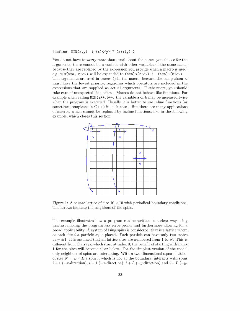
Figure 1: A square lattice of size 10 × 10 with periodical boundary conditions.The arrows indicate the neighbors of the spins.

The example illustrates how a program can be written in a clear way usingmacros, making the program less error-prone, and furthermore allowing for abroad applicability. A system of Ising spins is considered, that is a lattice whereat each site i a particle σi is placed. Each particle can have only two statesσi = ±1. It is assumed that all lattice sites are numbered from 1 to N . This isdifferent from C arrays, which start at index 0, the benefit of starting with index1 for the sites will become clear below. For the simplest version of the modelonly neighbors of spins are interacting. With a two-dimensional square latticeof size N = L × L a spin i, which is not at the boundary, interacts with spinsi + 1 (+x-direction), i − 1 (−x-direction), i + L (+y-direction) and i − L (−y-

22

direction). A spin at the boundary may interact with fewer neighbors when freeboundary conditions are assumed. With periodic boundary conditions (pbc),all spins have exactly 4 neighbors. In this case, a spin at the boundary interactsalso with the nearest mirror images, i.e. with the sites that are neighbors if youconsider the system repeated in each direction. For a 10 × 10 system spin 5,which is in the first row, interacts with spins 5 + 1 = 6, 5 − 1 = 4, 5 + 10 = 15and through the pbc with spin 95, see Fig. 1. The spin in the upper left corner,spin 1, interacts with spins 2, 11, 10 and 91. In a program pbc can be realizedby performing all calculations modulo L (for the ±x-directions) and modulo L2

(for the ±y-directions), respectively.This way of realizing the neighbor relations in a program has several disadvan-tages:

• You have to write the code everywhere where the neighbor relation isneeded. This makes the source code larger and less clear.

• When switching to free boundary conditions, you have to include furthercode to check whether a spin is at the boundary.

• Your code works only for one lattice type. If you want to extend theprogram to lattices of higher dimension you have to rewrite the code orprovide extra tests/calculations.

• Even more complicated would be an extension to different lattice struc-tures such as triangle or face-center cubic. This would make the programlook even more confusing.

An alternative is to write the program directly in a way it can cope with almostarbitrary lattice types. This can be achieved by setting up the neighbor relationin one special initialization subroutine (not discussed here) and storing it in anarray next[]. Then, the code outside the subroutine remains the same for alllattice types and dimensions. Since the code should work for all possible latticedimensions, the array next is one dimensional. It is assumed that each site hasnum n neighbors. Then the neighbors of site i can be stored in next[i*num n],

next[i*num n+1], . . ., next[i*num n+num n-1]. Please note that the sites arenumbered beginning with 1. This means, a system with N spins needs an ar-ray NEXT of size (N+1)*num n. When using free boundary conditions, missingneighbors can be set to 0. The access to the array can be made easier using amacro NEXT:

#define NEXT(i,r) next[(i)*num_n + r]

NEXT(i,r) contains the neighbor of spin i in direction r. For e.g. a quadraticsystem, r=0 is the +x-direction, r=1 the −x-direction, r=2 the +y-direction andr=3 the −y-direction. However, which convention you use depends on you, butyou should make sure you are consistent. For the case of a quadratic lattice,it is num n=4. Please note that whenever the macro NEXT is used, there mustbe a variable num_n defined, which stores the number of neighbors. You could

23

include num_n as a third parameter of the macro, but in this case a call of themacro looks slightly more confusing. Nevertheless, the way you define such amacro depends on your personal preferences.Please note that the NEXT macro cannot be realized by an inline function, incase you want to set values directly like in NEXT(i,0)=i+1. Also, when using aninline function, you would have to include all parameters explicitly, i.e. num_n

in the example. The last requirement could be circumvented by using globalvariables, but this is bad programming style as well.When the system is an Ising spin glass, the sign and magnitude of the interactionmay be different for each pair of spins. The interaction strengths can be storedin a similar way to the neighbor relation, e.g. in an array j[]. The access canbe simplified via the macro J :

#define J(i,r) j[(i)*num_n + r]

A subroutine for calculating the energy H =∑

〈i,j〉 Jijσiσj may look as follows,please note that the parameter N denotes the number of spins and the values ofthe spins are stored in the array sigma[]:

double spinglass_energy(int N, int num_n, int *next, int *j,

short int *sigma)

{

double energy = 0.0;

int i, r; /* counters */

for(i=1; i<=N; i++) /* loop over all lattice sites */

for(r=0; r<num_n; r++) /* loop over all neighbors */

energy += J(i,r)*sigma[i]*sigma[NEXT(i,r)];

return(energy/2); /* each pair has appeared twice in the sum */

}

For this piece of code the comments explaining the parameters and the purposeof the code are just missing for convenience. In the actual program it should beincluded.The code for spinglass energy() is very short and clear. It works for allkinds of lattices. Only the subroutine where the array next[] is set up hasto be rewritten when implementing a different type of lattice. This is true forall kinds of code realizing e.g. a Monte Carlo scheme or the calculation of aphysical quantity. For free boundary conditions, additionally sigma[0]=0 mustbe assigned to be consistent with the convention that missing neighbors havethe id 0. This is the reason, why the spin site numbering starts with index 1while C arrays start with index 0.

4.2 Make Files

If your software project grows larger, it will consist of several source-code files.Usually, there are many dependencies between the different files, e.g. a data

24

type defined in one header file can be used in several modules. Consequently,when changing one of your source files, it may be necessary to recompile severalparts of the program. In case you do not want to recompile your files every timeby hand, you can transfer this task to the make tool which can be found onUNIX operating systems. A complete description of the abilities of make can befound in Ref. [12]. You should look on the man page (type man make) or in thetexinfo file [13] as well. For other operating systems or software developmentenvironments, similar tools exists. Please consult the manuals in case you arenot working with a UNIX type of operating system.The basic idea of make is that you keep a file which contains all dependenciesbetween your source code files. Furthermore, it contains commands (e.g. thecompiler command) which generate the resulting files called targets , i.e. the finalprogram and/or object (.o) files. Each pair of dependencies and commands iscalled rule. The file containing all rules of a project is called makefile, usuallyit is named Makefile and should be placed in the directory where the sourcefiles are stored.A rule can be coded by two lines of the form

target : sources

<tab> command(s)

The first line contains the dependencies, the second one the commands. Thecommand line must begin with a tabulator symbol <tab>. It is allowed to haveseveral targets depending on the same sources. You can extend the lines withthe backslash “\” at the end of each line. The command line is allowed to beleft empty. An example of a dependency/command pair is

simulation.o: simulation.c simulation.h

<tab> cc -c simulation.c

This means that the file simulation.ohas to be compiled if either simulation.cor simulation.h have been changed. The make program is called by typingmake on the command line of a UNIX shell. It uses the date of the last changes,which is stored along with each file, to determine whether a rebuild of sometargets is necessary. Each time at least one of the source files are newer thanthe corresponding target files, the commands given after the <tab> are called.Specifically, the command is called, if the target file does not exist at all. Inthis special case, no source files have to be given after the colon in the first lineof the rule.It is also possible to generate meta rules, which e.g. tell how to treat all fileswhich have a specific suffix. Standard rules, how to treat files ending for examplewith .c are already included, but can be changed for each file by stating adifferent rule. This subject is covered in the man page of make.The make tool always tries to build only the first object of your makefile, unlessenforced by the dependencies. Hence, if you have to build several independentobject files object1, object2, object3, the whole compiling must be toggledby the first rule, thus your makefile should read like this

25

all: object1 object2 object3

object1: <sources of object1>

<tab> <command to generate object1>

object2: ...


object3 ...


It is not necessary to separate different rules by blank lines. Here it is justfor better readability. If you want to rebuild just e.g. object3, you can callmake object3. This allows several independent targets to be combined intoone makefile. When compiling programs via make, it is common to includethe target “clean” in the makefile such that all objects files are removed whenmake clean is called. Thus, the next call of make (without further arguments)compiles the whole program again from scratch. The rule for ‘clean‘ reads like

clean:

<tab> rm -f *.o

Also iterated dependencies are allowed, for example

object1: object2

object2: object3

<tab> ...

object3: ...

<tab> ...

The order of the rules is not important, except that make always starts withthe first target. Please note that the make tool is not just intended to managethe software development process and toggle compile commands. Any projectwhere some output files depend on some input files in an arbitrary way canbe controlled. For example you could control the setting of a book, where youhave text-files, figures, a bibliography and an index as input files. The differentchapters and finally the whole book are the target files.Furthermore, it is possible to define variables, sometimes also called macros.They have the format

variable=definition

Also variables belonging to your environment like $HOME can be referenced inthe makefile. The value of a variable can be used, similar to shells variables, byplacing a $ sign in front of the name of the variable, but you have to embrace

26

the name by (. . .) or {. . .}. There are some special variables, e.g. $@ holdsthe name of the target in each corresponding command line, here no braces arenecessary. The variable CC is predefined to hold the compiling command, youcan change it by including for example

CC=gcc

in the makefile. In the command part of a rule the compiler is called via $(CC).Thus, you can change your compiler for the whole project very quickly by al-tering just one line of the makefile.Finally, it will be shown what a typical makefile for a small software projectmight look like. The resulting program is called simulation. There are twoadditional modules init.c, run.c and the corresponding header .h files. Indatatypes.h types are defined which are used in all modules. Additionally, anexternal precompiled object file analysis.o in the directory $HOME/lib is to belinked, the corresponding header file is assumed to be stored in $HOME/include.For init.o and run.o no commands are given. In this case make applies thepredefined standard command for files having .o as suffix, which reads like

<tab> $(CC) $(CFLAGS) -c $@

where the variable CFLAGS may contain options passed to the compiler and isinitially empty. The makefile looks like this, please note that lines beginningwith “#” are comments.

#

# sample make file

#

OBJECTS=simulation.o init.o run.o

OBJECTSEXT=$(HOME)/lib/analysis.o

CC=gcc

CFLAGS=-g -Wall -I$(HOME)/include

LIBS=-lm

simulation: $(OBJECTS) $(OBJECTSEXT)

<tab> $(CC) $(CFLAGS) -o $@ $(OBJECTS) $(OBJECTSEXT) $(LIBS)

$(OBJECTS): datatypes.h

clean:

<tab> rm -f *.o

The first three lines are comments, then five variables OBJECTS, OBJECTSEXT,CC, CFLAGS and LIBS are assigned. The final part of the makefile are the rules.Please note that sometimes bugs are introduced, if the makefile is incomplete.For example consider a header file which is included in several code files, butthis is not mentioned in the makefile. Then, if you change e.g. a data type in the

27

header file, some of the code files might not be compiled again, especially thoseyou did not change. Thus the same objects files can be treated with differentformats in your program, yielding bugs which seem hard to explain. Hence,in case you encounter mysterious bugs, a make clean might help. But mostof the time, bugs which are hard to explain are due to errors in your memorymanagement. How to track down those bugs is explained in Sec. 7.The make tool exhibits many other features. For additional details, please con-sult the references given above.

4.3 Scripts

Scripts are even more general tools than make files. They are in fact smallprograms, but they are usually not compiled, i.e. they are quickly written butthey run slowly. Scripts can be used to perform many administration tasks likebacking up data, installing software or running simulation programs for manydifferent parameters. Here only an example concerning the last task is presented.For a general introduction to scripts, please refer to a book on UNIX/Linux.Assume that you have a simulation program called coversim21which calculatesvertex covers of graphs. In case you do not know what a vertex cover is, it doesnot matter, just regard it as one optimization problem characterized by someparameters. You want to run the program for a fixed graph size L, for a fixedconcentration c of the edges, average over num realizations and write the resultsto a file, which contains a string appendix in its name to distinguish it fromother output files. Furthermore, you want to iterate over different relative sizesx. Then you can use the following script run.scr:

#!/bin/bash

L=$1

c=$2

num=$3

appendix=$4

shift

shift

shift

shift

for x

do

${HOME}/cover/coversim21 -mag $L $c $x $num > \

mag_${c}_${x}${appendix}.out

done

The first line starting with “#” is a comment line, but it has a special meaning.It tells the operating system the language in which the script is written. In thiscase it is for the bash shell, the absolute pathname of the shell is given. EachUNIX shell has its own script language, you can use all commands which areallowed in the shell. There are also more elaborate script languages like perl orphyton, but they are not covered here.

28

Scripts can have command line arguments, which are referred via $1, $2, $2etc., the name of the script itself is stored in $0. Thus, in the lines 2 to 5, fourvariables are assigned. In general, you can use the arguments everywhere in thescript directly, i.e. it is not necessary to store them in other variables. It is donehere because in the next four lines the arguments $1 to $4 are thrown away byfour shift commands. Then, the argument which was on position five at thebeginning is stored in the first argument. Argument zero, containing the scriptname, is not affected by the shift.Next, the script enters a loop, given by “for x; do ... done”. This con-struction means that iteratively all remaining arguments are assigned to thevariable “x” and each time the body of the loop is executed. In this case, thesimulation is started with some parameters and the output directed to a file.Please note that you can state the loop parameters explicitly like in “for size

in 10 20 40 80 160; do ... done”.The above script can be called for example by

run.scr 100 0.5 1000 testA 0.20 0.22 0.24 0.26 0.28 0.30

which means that the graph size is 100, the fraction of edges is 0.5, the numberof realizations per run is 100, the string testA appears in the output file nameand the simulation is performed for the relative sizes 0.20, 0.22, 0.24, 0.26, 0.28,0.30.

5 Libraries

Libraries are collections of subroutines and data types, which can be used inother programs. There are libraries for numerical methods such as integrationor solving differential equations, for storing, sorting and accessing data, forfancy data types like lists or trees, for generating colorful graphics and forthousands of other applications. Some can be obtained for free, while other,usually specialized libraries have to be purchased. The use of libraries speedsup the software development process enormously, because you do not have toimplement every standard method by yourself. Hence, you should always checkwhether someone has done the jobs for you already, before starting to write aprogram. Here, two standard libraries are briefly presented, providing routineswhich are needed for most computer simulations.Nevertheless, sometimes it is inevitable to implement some methods by yourself.In this case, after the code has been proven to be reliable and useful for sometime, you can put it in a self-created library. How to create libraries is explainedin the last part of this section.

5.1 Numerical Recipes

The Numerical Recipes (NR) [3] contain a huge number of subroutines to solvestandard numerical problems. Among them are:

29

• solving linear equations

• performing interpolations

• evaluation and integration of functions

• solving nonlinear equations

• minimizing functions

• diagonalization of matrices

• Fourier transform

• solving ordinary and partial differential equations.

The algorithms included are all state of the art. There are several libraries ded-icated to similar problems, e.g. the library of the Numerical Algorithms Group[14] or the subroutines which are included with the Maple software package [15].To give you an impression how the subroutines can be used, just a short exampleis presented. Consider the case that a symmetrical matrix is given and that alleigenvalues are to be determined. For more information on the library thereader should consult Ref. [3]. There it is not only shown how the library canbe applied, but also all algorithms are explained.The program to calculate the eigenvalues reads as follows.

#include <stdio.h>

#include <stdlib.h>

#include "nrutil.h"

#include "nr.h"

int main(int argc, char *argv[])

{

float **m, *d, *e; /* matrix, two vectors */

long n = 10; /* size of matrix */

int i, j; /* loop counter */

m = matrix(1, n, 1, n); /* allocate matrix */

for(i=1; i<=n; i++) /* initialize matrix randomly */

for(j=i; j<=n; j++)

{

m[i][j] = drand48();

m[j][i] = m[i][j]; /* matrix must be symmetric here */

}

d = vector(1,n); /* contains diagonal elements */

e = vector(1,n); /* contains off diagonal elements */

tred2(m, n, d, e); /* convert symmetric m. -> tridiagonal */

tqli(d, e, n, m); /* calculate eigenvalues */

30

for(j=1; j<=n; j++) /* print result stored now in array ’d’*/

printf("ev %d = %f\n", j, d[j]);

free_vector(e, 1, n); /* give memory back */

free_vector(d, 1, n);

free_matrix(m, 1, n, 1, n);

return(0);

}

In the first part of the program, an n×n matrix is allocated via the subroutinematrix() which is provided by Numerical Recipes . It is standard to let a vectorstart with index 1, while in C usually a vector starts with index 0.In the second part a matrix is initialized randomly. Since the following subrou-tines work only for symmetric real matrices, the matrix is initialized symmet-rically. The Numerical Recipes also provide methods to diagonalize arbitrarymatrices, for simplicity this special case is chosen here .In the third part the main work is done by the Numerical Recipes subrou-tines tred2() and tqli(). First, the matrix is written in tridiagonal form bya Householder transformation (tred2()) and then the actual eigenvalues arecalculated by calling tqli(d, e, n, m). The eigenvalues are returned in thevector d[] and the eigenvectors in the matrix m[][] (not used here), which isoverwritten. Finally the memory allocated for the matrix and the vectors isfreed again.This small example should be sufficient to show how simply the subroutinesfrom the Numerical Recipes can be incorporated into a program. When youhave a problem of this kind you should always consult the NR library first,before starting to write code by yourself.

5.2 LEDA

While the Numerical Recipes are dedicated to numerical problems, the Libraryof Efficient Data types and Algorithms (LEDA) [4] can help a great deal inwriting efficient programs in general. It is written in C++, but it can be usedby C style programmers as well via mixing C++ calls to LEDA subroutineswithin C code. LEDA contains many basic and advanced data types such as:

• strings

• numbers of arbitrary precision

• one- and two-dimensional arrays

• lists and similar objects like stacks or queues

• sets

• trees

• graphs (directed and undirected, also labeled)

31

• dictionaries, there you can store objects with arbitrary key words as indices

• data types for two and three dimensional geometries, like points, segmentsor spheres

For most data types, it is possible to create arbitrary complex structures by usingtemplates. For example you can make lists of self defined structures or stacks oftrees. The most efficient implementations known in literature so far are taken forall data structures. Usually, you can choose between different implementations,to match special requirements. For every data type, all necessary operationsare included; e.g. for lists: creating, appending, splitting, printing and deletinglists as well as inserting, searching, sorting and deleting elements in a list, alsoiterating over all elements of a list. The major part of the library is dedicated tographs and related algorithms. You will find for example subroutines to calculatestrongly connected components, shortest paths, maximum flows, minimum costflows and (minimum) matchings.Here again, just a short example is given to illustrate how the library can beutilized and to show how easy LEDA can be used. A list of a self definedclass Mydatatype is considered. Each element contains the data entries info

and flag. In the first part of the program below, the class Mydatatype ispartly defined. Please note that input and output stream operators <</>> mustbe provided to be able to create a list of Mydatatype elements, otherwise theprogram will not compile. In the main part of the program a list is defined viathe LEDA data type list. Elements are inserted into the list with append().Finally an iteration over all list elements is performed using the LEDA macroforall. The program leda test.cc reads as follows:

#include <iostream.h>

#include <LEDA/list.h>

class Mydatatype // self defined example class

{

public:

int info; // user data 1

short int flag; // user data 2

Mydatatype() {info=0; flag=0;}; // constructor

~Mydatatype() {}; // destructor

friend ostream& operator<<(ostream& O, const Mydatatype& dt)

{ O << "info: " << dt.info << " flag: " << dt.flag << "\n";

return(O);}; // output operator

friend istream& operator>>(istream &I, Mydatatype& dt)

{return(I);}; // dummy

};

32


{

list<Mydatatype> l; // list with elements of ’Mydatatype’

Mydatatype element;

int t;

for(t=0; t<10; t++) // create list

{

element.info = t;

element.flag = t%2;

l.append(element);

}

forall(element, l) // iterate over all elements

if(element.flag) // print only ’even’ elements

cout << element;

return(0);

}

The program has to be compiled with a C++ compiler. Depending on yoursystem, you have to specify some compiler flags to include LEDA, please con-sult your systems documentation or the system administrator. The compilecommand may look like this:

g++ -I$LEDAROOT/incl -L$LEDAROOT -o leda_test leda_test.cc -lG -lL

The -I flag specifies where the compiler searches for header files like LEDA/list.h,the -L flag tells where the libraries (-lG -lL) are located. The environmentvariable LEDAROOT must point to the directory where LEDA is stored in yoursystem.Please note that using Numerical Recipes and LEDA together results in conflicts,since the objects vector and matrix are defined in both libraries. You cancircumvent this problem by taking the source code of Numerical Recipes (here:nrutil.c, nrutil.h) and rename the subroutines matrix() and vector(),compile again and include nrutil.o directly in your program.Here, it should be stressed: Before trying to write everything by yourself, youshould check whether someone else has done it for you already. LEDA is ahighly effective and very convenient tool. It will save you a lot of time andeffort when you use it for your program development.

5.3 Creating your own Libraries

Although many useful libraries are available, sometimes you have to write somecode by yourself. Over the years you will collect many subroutines, which –if properly designed – can be included in other programs, in which case it isconvenient to put these subroutines in a library. Then you do not have to includethe object file every time you compile one of your programs. If your self-created

33

library is put in a standard search path, you can access it like a system library,you even do not have to remember where the object file is stored.To create a library you must have an object file, e.g. tasks.o, and a header filetasks.hwhere all data types and function prototypes are defined. Furthermore,to facilitate the use of the library, you should write a man page, which is notnecessary for technical reasons but results in a more convenient usage of yourlibrary, particularly should other people want to benefit from it. To learn howto write a man page you should consult man man and have a look at the sourcecode of some man pages, they are stored e.g. in /usr/man.A library is created with the UNIX command ar. To include tasks.o in yourlibrary libmy.a you have to enter

ar r libmy.a tasks.o

In a library several object files may be collected. The option “r” replaces thegiven object files, if they already belong to the library, otherwise they are added.If the library does not exist yet it is created. For more options, please refer tothe man page of ar.After including an object file, you have to update an internal object table of thelibrary. This is done by

ar s libmy.a

Now you can compile a program prog.c using your library via

cc -o prog prog.c libmy.a

In case libmy.a contains several object files, it saves some typing by just writinglibmy.a, furthermore you do not have to remember the names of all your objectfiles.To make the handling of the library more comfortable, you can create a directory,e.g. ∼/lib and put your libraries there. Additionally, you should create thedirectory ∼/include where all personal header files can be collected. Thenyour compile command may look like this:

cc -o prog prog.c -I$HOME/include -L$HOME/lib -lmy

The option -I states the search path for additional header files, the -L optiontells the linker where your libraries are stored and via -lmy the library libmy.a

is actually included. Please note that the prefix lib and the postfix .a areomitted with the -l option. Finally, it should be pointed out, that the compilercommand given above works in all directories, once you have set up the structureas explained. Hence, you do not have to remember directories or names of objectfiles.

6 Random Numbers

For many simulations in physics, random numbers are necessary. Quite oftenthe model itself exhibits random parameters which remain fixed throughout

34

the simulation, one speaks of quenched disorder . A famous example are spinglasses. In this case one has to perform an average over different realizations ofthe disorder, to obtain physical quantities.But even when the system which is treated is not random, very often randomnumbers are required by the algorithms, e.g. to realize a finite-temperature en-semble or when using randomized algorithms. In this section an introduction tothe generation of random numbers is given. First it is explained how they canbe generated at all on a computer. Then, different methods for obtaining num-bers are explained, which obey a given distribution: the inversion method , theBox-Muller method and the rejection method . More comprehensive informationabout these and similar techniques can be found in Refs. [3, 16].In this section it is assumed that you are familiar with the basic concepts ofprobability theory and statistics.

6.1 Generating Random Numbers

First, it should be pointed out that standard computers are deterministic ma-chines. Thus, it is completely impossible to generate true random numbers, atleast not without the help of the user. It is for example possible to measurethe time interval between successive keystrokes, which is randomly distributedby nature. But they depend heavily on the current user and it is not possibleto reproduce an experiment in exactly the same way. This is the reason whypseudo random numbers are usually taken. They are generated by deterministicrules, but they look like and have many of the properties of true random num-bers. One would like to have a random number generator rand(), such thateach possible number has the same probability of occurrence. Each time rand()is called, a new random number is returned. Additionally, if two numbers ri, rk

differ only slightly, the random numbers ri+1, rk+1 returned by the respectivesubsequent calls should have a low correlation.The simplest methods to generate pseudo random numbers are linear congruen-tial generators . They generate a sequence I1, I2, . . . of integer numbers between0 and m − 1 by a recursive recipe:

In+1 = (aIn + c)modm (1)

To generate random numbers r distributed in the interval [0, 1) one has to dividethe current random number by m. It is desirable to obtain equally distributedvalues in the interval, i.e. a uniform distribution. Below, you will see, howrandom numbers obeying other distributions can be generated from uniformlydistributed numbers.The real art is to choose the parameters a, c, m in a way that “good” randomnumbers are obtained, where “good” means “with less correlations”. In the pastseveral results from simulations have been turned out to be wrong, because ofthe application of bad random number generators [17].

35

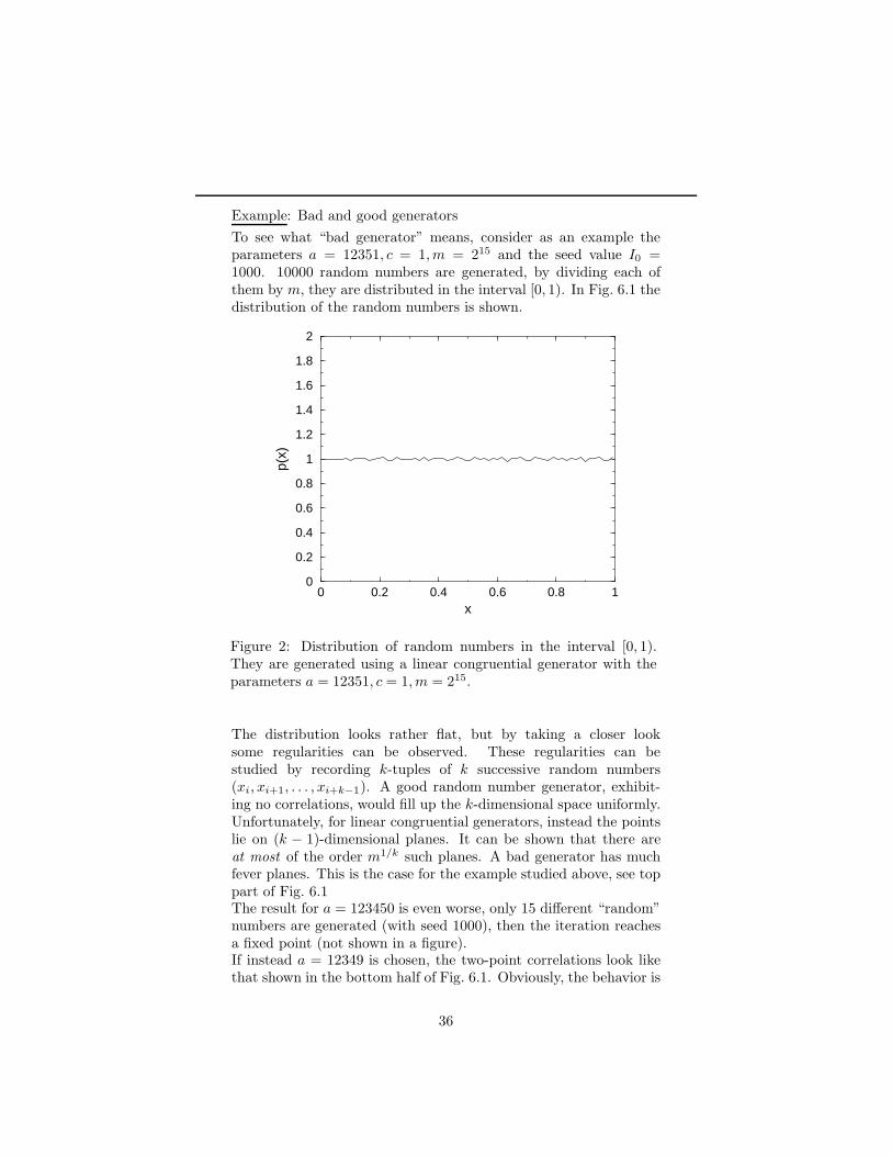
Example: Bad and good generators

To see what “bad generator” means, consider as an example theparameters a = 12351, c = 1, m = 215 and the seed value I0 =1000. 10000 random numbers are generated, by dividing each ofthem by m, they are distributed in the interval [0, 1). In Fig. 6.1 thedistribution of the random numbers is shown.

0 0.2 0.4 0.6 0.8 1x

0

0.2

0.4

0.6

0.8

1

1.2

1.4

1.6

1.8

2

p(x)

Figure 2: Distribution of random numbers in the interval [0, 1).They are generated using a linear congruential generator with theparameters a = 12351, c = 1, m = 215.

The distribution looks rather flat, but by taking a closer looksome regularities can be observed. These regularities can bestudied by recording k-tuples of k successive random numbers(xi, xi+1, . . . , xi+k−1). A good random number generator, exhibit-ing no correlations, would fill up the k-dimensional space uniformly.Unfortunately, for linear congruential generators, instead the pointslie on (k − 1)-dimensional planes. It can be shown that there areat most of the order m1/k such planes. A bad generator has muchfever planes. This is the case for the example studied above, see toppart of Fig. 6.1The result for a = 123450 is even worse, only 15 different “random”numbers are generated (with seed 1000), then the iteration reachesa fixed point (not shown in a figure).If instead a = 12349 is chosen, the two-point correlations look likethat shown in the bottom half of Fig. 6.1. Obviously, the behavior is

36

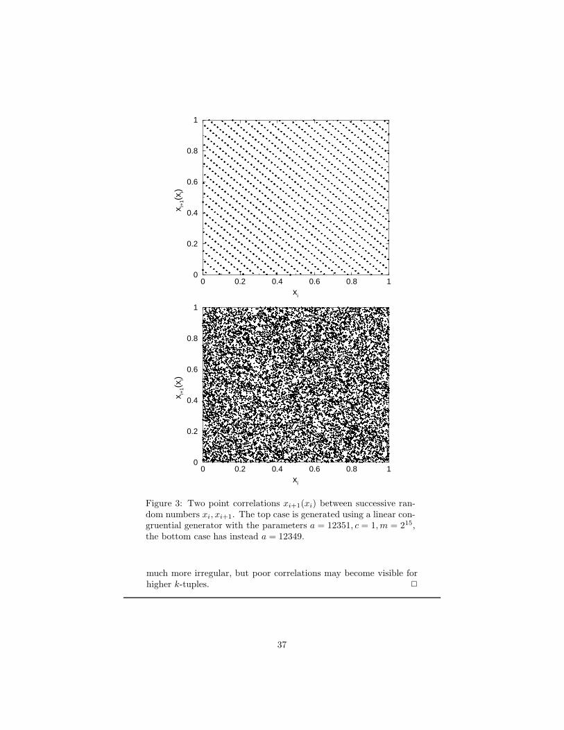
0 0.2 0.4 0.6 0.8 1xi

0

0.2

0.4

0.6

0.8

1

x i+1(

x i)

0 0.2 0.4 0.6 0.8 1xi

0

0.2

0.4

0.6

0.8

1

x i+1(

x i)

Figure 3: Two point correlations xi+1(xi) between successive ran-dom numbers xi, xi+1. The top case is generated using a linear con-gruential generator with the parameters a = 12351, c = 1, m = 215,the bottom case has instead a = 12349.

much more irregular, but poor correlations may become visible forhigher k-tuples. 2

37

A generator which has passed several theoretical test is a = 75 = 16807, m =231 − 1, c = 0. When implementing this generator you have to be careful,because during the calculation numbers are generated which do not fit into 32bit. A clever implementation is presented in Ref. [3]. Finally, it should bestressed that this generator, like all linear congruential generators, has the low-order bits much less random than the high-order bits. For that reason, whenyou want to generate integer numbers in an interval [1,N], you should use

r = 1+(int) (N*(I_n)/m);

instead of using the modulo operation as with r=1+(I n % N);.So far it has been shown how random numbers can be generated which are dis-tributed uniformly in the interval [0, 1). In general, one is interested in obtainingrandom numbers which are distributed according to a given probability distri-bution with density p(z). In the next sections, several techniques performingthis task for continuous probability distributions are presented.In case of discrete distributions, one has to create a table of the possible out-comes with their probabilities pi. To draw a number, one has to draw a randomnumber u which is uniformly distributed in [0, 1) and take the entry j of the

table such that the sum∑j

i=1 pi of the preceding probabilities is larger than u,

but∑j−1

i=1 pi < u. In the following, we concentrate on techniques for generatingcontinuous random variables.

6.2 Inversion Method

Given is a random number generator drand() which is assumed to generaterandom numbers U which are distributed uniformly in [0, 1). The aim is togenerate random numbers Z with probability density p(z). The correspondingdistribution function is

P (z) ≡ Prob(Z ≤ z) ≡∫ z

−∞

dz′p(z′) (2)

The target is to find a function g(X), such that after the transformation Z =g(U), the values of Z are distributed according to (2). It is assumed that g canbe inverted and is strongly monotonically increasing, then one obtains

P (z) = Prob(Z ≤ z) = Prob(g(U) ≤ z) = Prob(U ≤ g−1(z)) (3)

Since the distribution function F (u) = Prob(U ≤ u) for a uniformly distributedvariable is just F (u) = u (u ∈ [0, 1]), one obtains P (z) = g−1(z). Thus, one justhas to choose g(z) = P−1(z) for the transformation function, in order to obtainrandom numbers, which are distributed according the probability distributionP (z). Of course, this only works if P can be inverted.

38

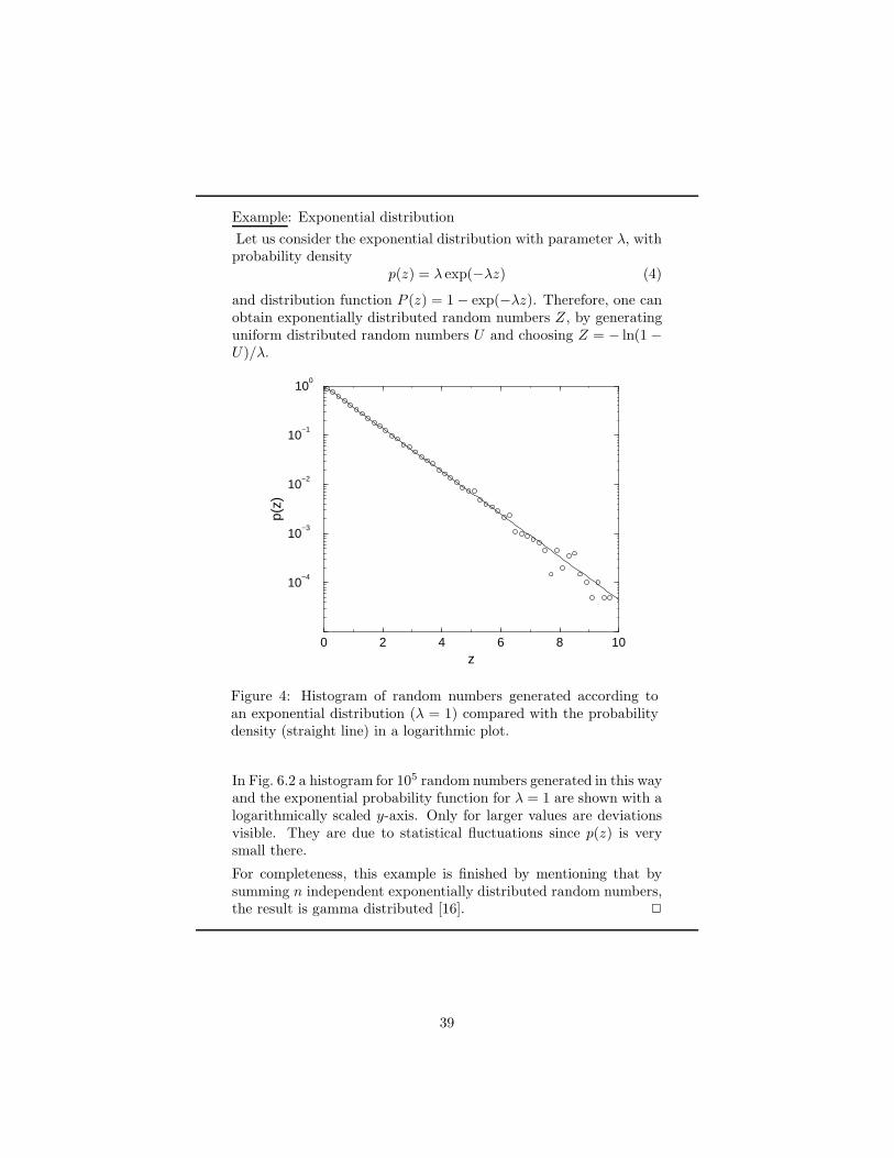
Example: Exponential distribution

Let us consider the exponential distribution with parameter λ, withprobability density

p(z) = λ exp(−λz) (4)

and distribution function P (z) = 1 − exp(−λz). Therefore, one canobtain exponentially distributed random numbers Z, by generatinguniform distributed random numbers U and choosing Z = − ln(1 −U)/λ.

0 2 4 6 8 10z

10−4

10−3

10−2

10−1

100

p(z)

Figure 4: Histogram of random numbers generated according toan exponential distribution (λ = 1) compared with the probabilitydensity (straight line) in a logarithmic plot.

In Fig. 6.2 a histogram for 105 random numbers generated in this wayand the exponential probability function for λ = 1 are shown with alogarithmically scaled y-axis. Only for larger values are deviationsvisible. They are due to statistical fluctuations since p(z) is verysmall there.

For completeness, this example is finished by mentioning that bysumming n independent exponentially distributed random numbers,the result is gamma distributed [16]. 2

39

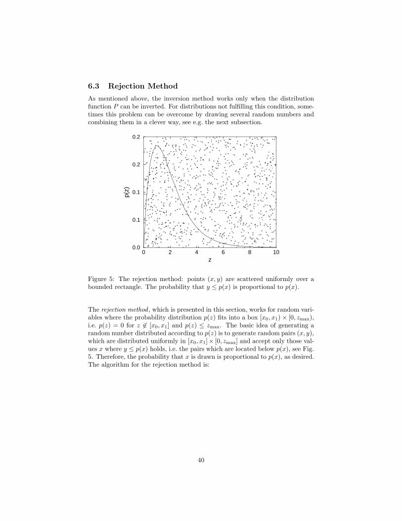
6.3 Rejection Method

As mentioned above, the inversion method works only when the distributionfunction P can be inverted. For distributions not fulfilling this condition, some-times this problem can be overcome by drawing several random numbers andcombining them in a clever way, see e.g. the next subsection.

0 2 4 6 8 10z

0.0

0.1

0.1

0.2

0.2

p(z)

Figure 5: The rejection method: points (x, y) are scattered uniformly over abounded rectangle. The probability that y ≤ p(x) is proportional to p(x).

The rejection method , which is presented in this section, works for random vari-ables where the probability distribution p(z) fits into a box [x0, x1) × [0, zmax),i.e. p(z) = 0 for z 6∈ [x0, x1] and p(z) ≤ zmax. The basic idea of generating arandom number distributed according to p(z) is to generate random pairs (x, y),which are distributed uniformly in [x0, x1]× [0, zmax] and accept only those val-ues x where y ≤ p(x) holds, i.e. the pairs which are located below p(x), see Fig.5. Therefore, the probability that x is drawn is proportional to p(x), as desired.The algorithm for the rejection method is:

40

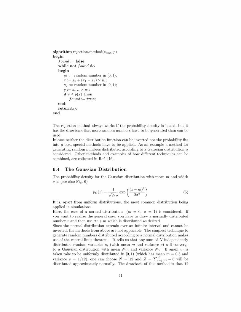
algorithm rejection method(zmax, p)begin

found := false;while not found dobegin

u1 := random number in [0, 1);x := x0 + (x1 − x0) × u1;u2 := random number in [0, 1);y := zmax × u2;if y ≤ p(x) then

found := true;end;return(x);

end

The rejection method always works if the probability density is boxed, but ithas the drawback that more random numbers have to be generated than can beused.In case neither the distribution function can be inverted nor the probability fitsinto a box, special methods have to be applied. As an example a method forgenerating random numbers distributed according to a Gaussian distribution isconsidered. Other methods and examples of how different techniques can becombined, are collected in Ref. [16].

6.4 The Gaussian Distribution

The probability density for the Gaussian distribution with mean m and widthσ is (see also Fig. 6)

pG(z) =1√2πσ

exp

(

(z − m)2

2σ2

)

(5)

It is, apart from uniform distributions, the most common distribution beingapplied in simulations.Here, the case of a normal distribution (m = 0, σ = 1) is considered. Ifyou want to realize the general case, you have to draw a normally distributednumber z and then use σz + m which is distributed as desired.Since the normal distribution extends over an infinite interval and cannot beinverted, the methods from above are not applicable. The simplest technique togenerate random numbers distributed according to a normal distribution makesuse of the central limit theorem. It tells us that any sum of N independentlydistributed random variables ui (with mean m and variance v) will convergeto a Gaussian distribution with mean Nm and variance Nv. If again ui istaken take to be uniformly distributed in [0, 1) (which has mean m = 0.5 and

variance v = 1/12), one can choose N = 12 and Z =∑12

i=1 ui − 6 will bedistributed approximately normally. The drawback of this method is that 12

41

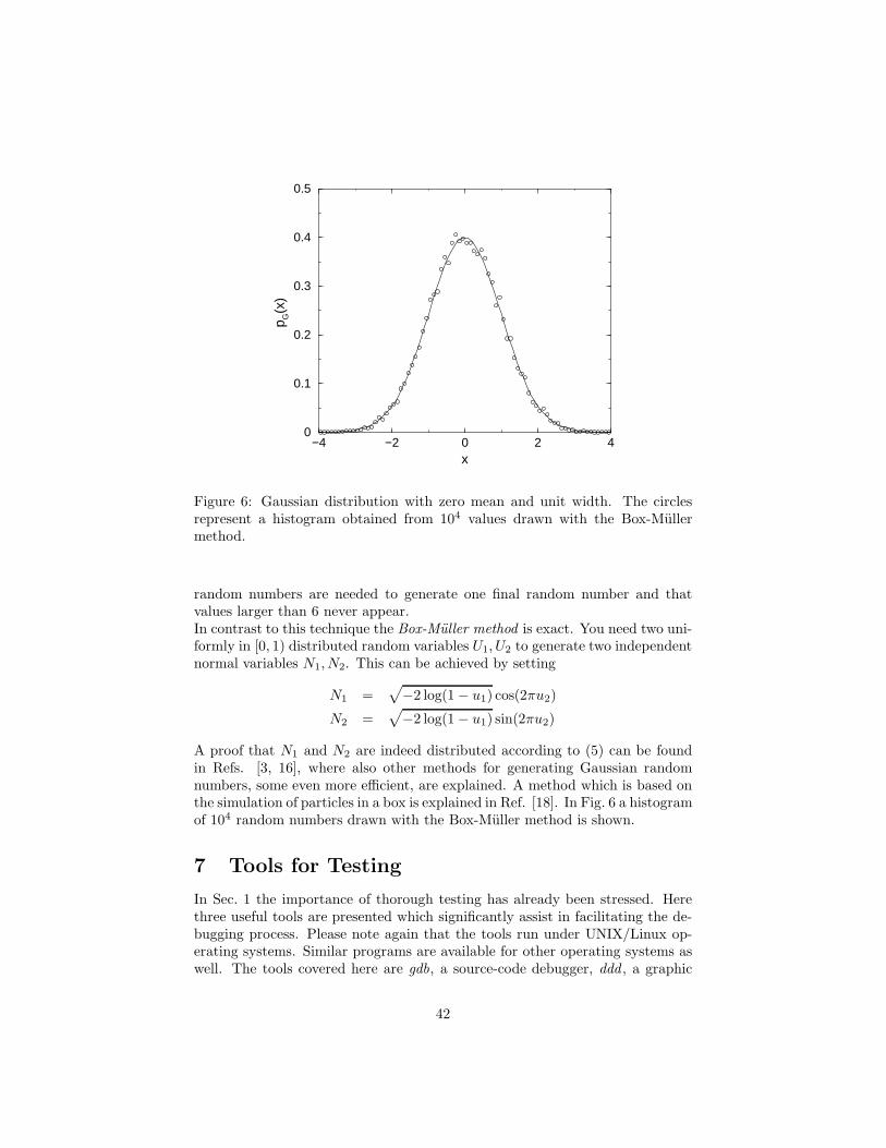
−4 −2 0 2 4x

0

0.1

0.2

0.3

0.4

0.5

p G(x

)

Figure 6: Gaussian distribution with zero mean and unit width. The circlesrepresent a histogram obtained from 104 values drawn with the Box-Mullermethod.

random numbers are needed to generate one final random number and thatvalues larger than 6 never appear.In contrast to this technique the Box-Muller method is exact. You need two uni-formly in [0, 1) distributed random variables U1, U2 to generate two independentnormal variables N1, N2. This can be achieved by setting

N1 =√

−2 log(1 − u1) cos(2πu2)

N2 =√

−2 log(1 − u1) sin(2πu2)

A proof that N1 and N2 are indeed distributed according to (5) can be foundin Refs. [3, 16], where also other methods for generating Gaussian randomnumbers, some even more efficient, are explained. A method which is based onthe simulation of particles in a box is explained in Ref. [18]. In Fig. 6 a histogramof 104 random numbers drawn with the Box-Muller method is shown.

7 Tools for Testing

In Sec. 1 the importance of thorough testing has already been stressed. Herethree useful tools are presented which significantly assist in facilitating the de-bugging process. Please note again that the tools run under UNIX/Linux op-erating systems. Similar programs are available for other operating systems aswell. The tools covered here are gdb, a source-code debugger, ddd , a graphic

42

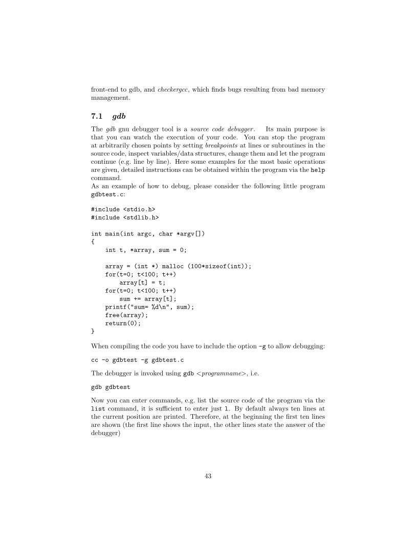
front-end to gdb, and checkergcc, which finds bugs resulting from bad memorymanagement.

7.1 gdb

The gdb gnu debugger tool is a source code debugger . Its main purpose isthat you can watch the execution of your code. You can stop the programat arbitrarily chosen points by setting breakpoints at lines or subroutines in thesource code, inspect variables/data structures, change them and let the programcontinue (e.g. line by line). Here some examples for the most basic operationsare given, detailed instructions can be obtained within the program via the helpcommand.As an example of how to debug, please consider the following little programgdbtest.c:

#include <stdio.h>

#include <stdlib.h>


{

int t, *array, sum = 0;

array = (int *) malloc (100*sizeof(int));

for(t=0; t<100; t++)

array[t] = t;

for(t=0; t<100; t++)

sum += array[t];

printf("sum= %d\n", sum);

free(array);

return(0);

}

When compiling the code you have to include the option -g to allow debugging:

cc -o gdbtest -g gdbtest.c

The debugger is invoked using gdb <programname>, i.e.

gdb gdbtest

Now you can enter commands, e.g. list the source code of the program via thelist command, it is sufficient to enter just l. By default always ten lines atthe current position are printed. Therefore, at the beginning the first ten linesare shown (the first line shows the input, the other lines state the answer of thedebugger)

43

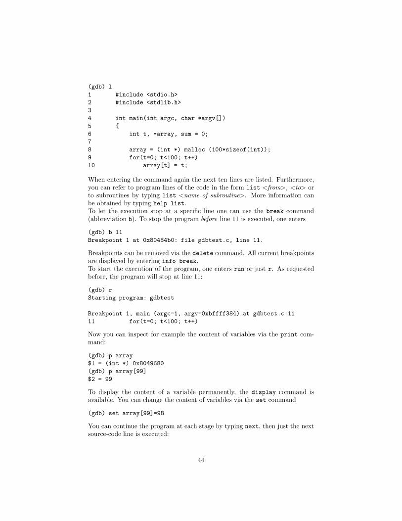
(gdb) l

1 #include <stdio.h>

2 #include <stdlib.h>

3

4 int main(int argc, char *argv[])

5 {

6 int t, *array, sum = 0;

7

8 array = (int *) malloc (100*sizeof(int));

9 for(t=0; t<100; t++)

10 array[t] = t;

When entering the command again the next ten lines are listed. Furthermore,you can refer to program lines of the code in the form list <from>, <to> orto subroutines by typing list <name of subroutine>. More information canbe obtained by typing help list.To let the execution stop at a specific line one can use the break command(abbreviation b). To stop the program before line 11 is executed, one enters

(gdb) b 11

Breakpoint 1 at 0x80484b0: file gdbtest.c, line 11.

Breakpoints can be removed via the delete command. All current breakpointsare displayed by entering info break.To start the execution of the program, one enters run or just r. As requestedbefore, the program will stop at line 11:

(gdb) r

Starting program: gdbtest

Breakpoint 1, main (argc=1, argv=0xbffff384) at gdbtest.c:11

11 for(t=0; t<100; t++)

Now you can inspect for example the content of variables via the print com-mand:

(gdb) p array

$1 = (int *) 0x8049680

(gdb) p array[99]

$2 = 99

To display the content of a variable permanently, the display command isavailable. You can change the content of variables via the set command

(gdb) set array[99]=98

You can continue the program at each stage by typing next, then just the nextsource-code line is executed:

44

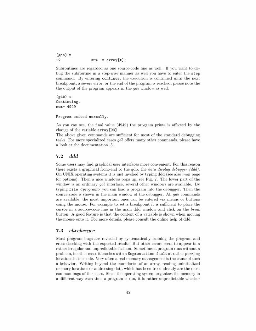
(gdb) n

12 sum += array[t];

Subroutines are regarded as one source-code line as well. If you want to de-bug the subroutine in a step-wise manner as well you have to enter the step

command. By entering continue, the execution is continued until the nextbreakpoint, a severe error, or the end of the program is reached, please note thethe output of the program appears in the gdb window as well:

(gdb) c

Continuing.

sum= 4949

Program exited normally.

As you can see, the final value (4949) the program prints is affected by thechange of the variable array[99].The above given commands are sufficient for most of the standard debuggingtasks. For more specialized cases gdb offers many other commands, please havea look at the documentation [5].

7.2 ddd

Some users may find graphical user interfaces more convenient. For this reasonthere exists a graphical front-end to the gdb, the data display debugger (ddd).On UNIX operating systems it is just invoked by typing ddd (see also man pagefor options). Then a nice windows pops up, see Fig. 7. The lower part of thewindow is an ordinary gdb interface, several other windows are available. Bytyping file <program> you can load a program into the debugger. Then thesource code is shown in the main window of the debugger. All gdb commandsare available, the most important ones can be entered via menus or buttonsusing the mouse. For example to set a breakpoint it is sufficient to place thecursor in a source-code line in the main ddd window and click on the breakbutton. A good feature is that the content of a variable is shown when movingthe mouse onto it. For more details, please consult the online help of ddd.

7.3 checkergcc

Most program bugs are revealed by systematically running the program andcross-checking with the expected results. But other errors seem to appear in arather irregular and unpredictable fashion. Sometimes a program runs without aproblem, in other cases it crashes with a Segmentation fault at rather puzzlinglocations in the code. Very often a bad memory management is the cause of sucha behavior. Writing beyond the boundaries of an array, reading uninitializedmemory locations or addressing data which has been freed already are the mostcommon bugs of this class. Since the operating system organizes the memory ina different way each time a program is run, it is rather unpredictable whether

45

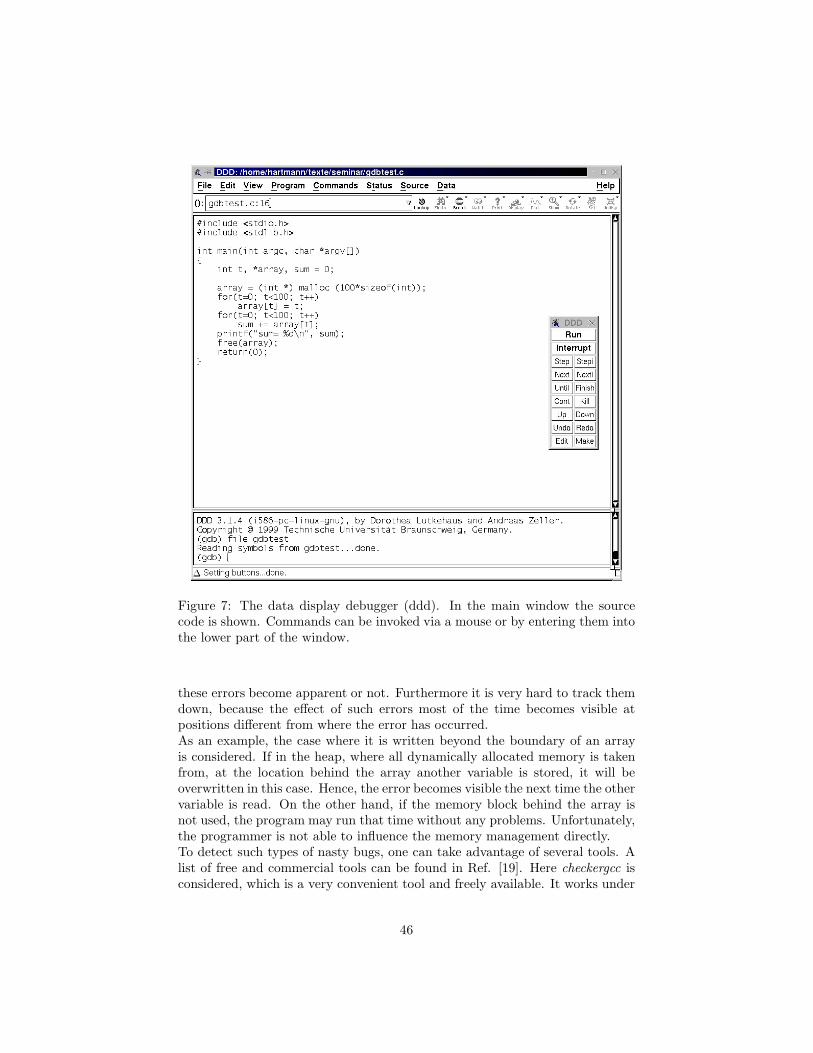
Figure 7: The data display debugger (ddd). In the main window the sourcecode is shown. Commands can be invoked via a mouse or by entering them intothe lower part of the window.

these errors become apparent or not. Furthermore it is very hard to track themdown, because the effect of such errors most of the time becomes visible atpositions different from where the error has occurred.As an example, the case where it is written beyond the boundary of an arrayis considered. If in the heap, where all dynamically allocated memory is takenfrom, at the location behind the array another variable is stored, it will beoverwritten in this case. Hence, the error becomes visible the next time the othervariable is read. On the other hand, if the memory block behind the array isnot used, the program may run that time without any problems. Unfortunately,the programmer is not able to influence the memory management directly.To detect such types of nasty bugs, one can take advantage of several tools. Alist of free and commercial tools can be found in Ref. [19]. Here checkergcc isconsidered, which is a very convenient tool and freely available. It works under

46

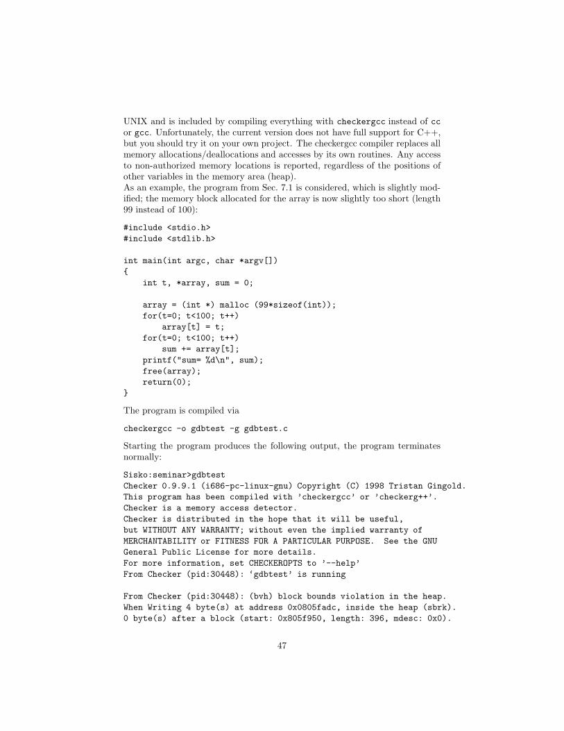
UNIX and is included by compiling everything with checkergcc instead of ccor gcc. Unfortunately, the current version does not have full support for C++,but you should try it on your own project. The checkergcc compiler replaces allmemory allocations/deallocations and accesses by its own routines. Any accessto non-authorized memory locations is reported, regardless of the positions ofother variables in the memory area (heap).As an example, the program from Sec. 7.1 is considered, which is slightly mod-ified; the memory block allocated for the array is now slightly too short (length99 instead of 100):

#include <stdio.h>

#include <stdlib.h>


{

int t, *array, sum = 0;

array = (int *) malloc (99*sizeof(int));

for(t=0; t<100; t++)

array[t] = t;

for(t=0; t<100; t++)

sum += array[t];

printf("sum= %d\n", sum);

free(array);

return(0);

}

The program is compiled via

checkergcc -o gdbtest -g gdbtest.c

Starting the program produces the following output, the program terminatesnormally:

Sisko:seminar>gdbtest

Checker 0.9.9.1 (i686-pc-linux-gnu) Copyright (C) 1998 Tristan Gingold.

This program has been compiled with ’checkergcc’ or ’checkerg++’.

Checker is a memory access detector.

Checker is distributed in the hope that it will be useful,

but WITHOUT ANY WARRANTY; without even the implied warranty of

MERCHANTABILITY or FITNESS FOR A PARTICULAR PURPOSE. See the GNU

General Public License for more details.

For more information, set CHECKEROPTS to ’--help’

From Checker (pid:30448): ‘gdbtest’ is running

From Checker (pid:30448): (bvh) block bounds violation in the heap.

When Writing 4 byte(s) at address 0x0805fadc, inside the heap (sbrk).

0 byte(s) after a block (start: 0x805f950, length: 396, mdesc: 0x0).

47

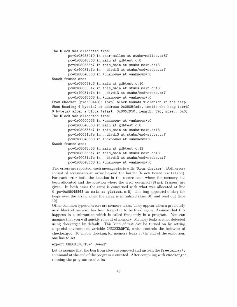
The block was allocated from:

pc=0x080554f9 in chkr_malloc at stubs-malloc.c:57

pc=0x08048863 in main at gdbtest.c:8

pc=0x080555a7 in this_main at stubs-main.c:13

pc=0x40031c7e in __divdi3 at stubs/end-stubs.c:7

pc=0x08048668 in *unknown* at *unknown*:0

Stack frames are:

pc=0x080489c3 in main at gdbtest.c:10




From Checker (pid:30448): (bvh) block bounds violation in the heap.

When Reading 4 byte(s) at address 0x0805fadc, inside the heap (sbrk).

0 byte(s) after a block (start: 0x805f950, length: 396, mdesc: 0x0).

The block was allocated from:






Stack frames are:

pc=0x08048c55 in main at gdbtest.c:12




Two errors are reported, each message starts with “From checker”. Both errorsconsist of accesses to an array beyond the border (block bound violation).For each error both the location in the source code where the memory hasbeen allocated and the location where the error occurred (Stack frames) aregiven. In both cases the error is concerned with what was allocated at line8 (pc=0x08048863 in main at gdbtest.c:8). The bug appeared during theloops over the array, when the array is initialized (line 10) and read out (line12).Other common types of errors are memory leaks. They appear when a previouslyused block of memory has been forgotten to be freed again. Assume that thishappens in a subroutine which is called frequently in a program. You canimagine that you will quickly run out of memory. Memory leaks are not detectedusing checkergcc by default. This kind of test can be turned on by settinga special environment variable CHECKEROPTS, which controls the behavior ofcheckergcc. To enable checking for memory leaks at the end of the execution,one has to set

export CHECKEROPTS="-D=end"

Let us assume that the bug from above is removed and instead the free(array);command at the end of the program is omitted. After compiling with checkergcc,running the program results in:

48

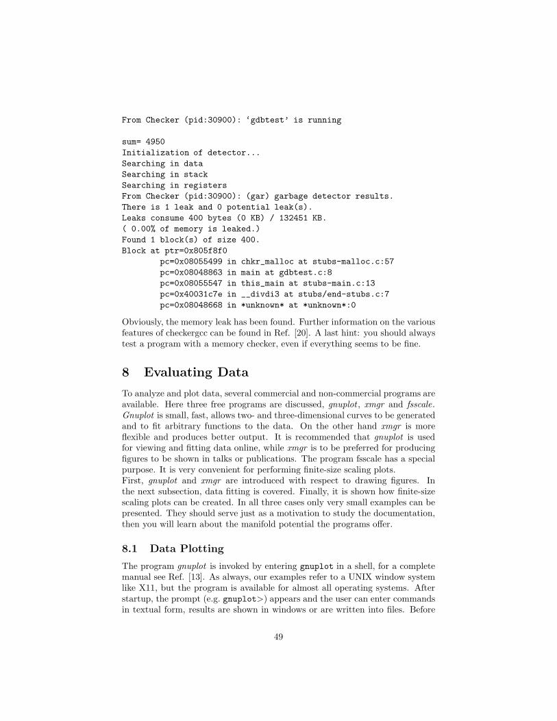
From Checker (pid:30900): ‘gdbtest’ is running

sum= 4950

Initialization of detector...

Searching in data

Searching in stack

Searching in registers

From Checker (pid:30900): (gar) garbage detector results.

There is 1 leak and 0 potential leak(s).

Leaks consume 400 bytes (0 KB) / 132451 KB.

( 0.00% of memory is leaked.)

Found 1 block(s) of size 400.

Block at ptr=0x805f8f0

pc=0x08055499 in chkr_malloc at stubs-malloc.c:57


pc=0x08055547 in this_main at stubs-main.c:13



Obviously, the memory leak has been found. Further information on the variousfeatures of checkergcc can be found in Ref. [20]. A last hint: you should alwaystest a program with a memory checker, even if everything seems to be fine.

8 Evaluating Data

To analyze and plot data, several commercial and non-commercial programs areavailable. Here three free programs are discussed, gnuplot , xmgr and fsscale.Gnuplot is small, fast, allows two- and three-dimensional curves to be generatedand to fit arbitrary functions to the data. On the other hand xmgr is moreflexible and produces better output. It is recommended that gnuplot is usedfor viewing and fitting data online, while xmgr is to be preferred for producingfigures to be shown in talks or publications. The program fsscale has a specialpurpose. It is very convenient for performing finite-size scaling plots.First, gnuplot and xmgr are introduced with respect to drawing figures. Inthe next subsection, data fitting is covered. Finally, it is shown how finite-sizescaling plots can be created. In all three cases only very small examples can bepresented. They should serve just as a motivation to study the documentation,then you will learn about the manifold potential the programs offer.

8.1 Data Plotting

The program gnuplot is invoked by entering gnuplot in a shell, for a completemanual see Ref. [13]. As always, our examples refer to a UNIX window systemlike X11, but the program is available for almost all operating systems. Afterstartup, the prompt (e.g. gnuplot>) appears and the user can enter commandsin textual form, results are shown in windows or are written into files. Before

49

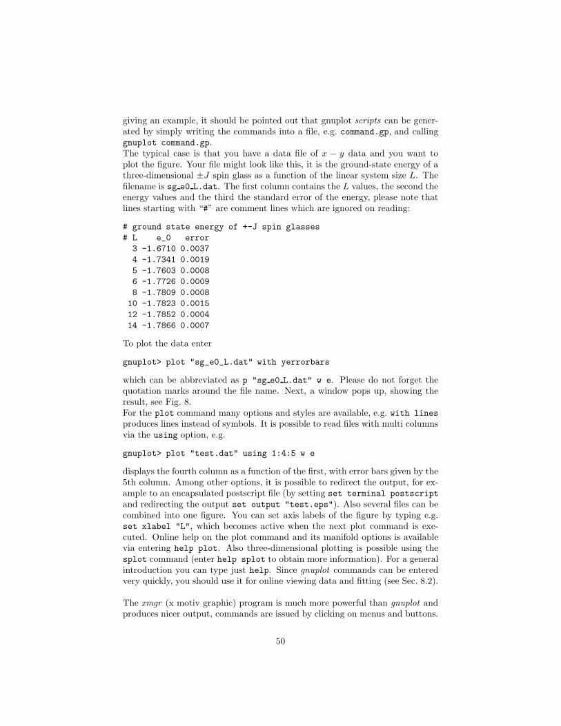
giving an example, it should be pointed out that gnuplot scripts can be gener-ated by simply writing the commands into a file, e.g. command.gp, and callinggnuplot command.gp.The typical case is that you have a data file of x − y data and you want toplot the figure. Your file might look like this, it is the ground-state energy of athree-dimensional ±J spin glass as a function of the linear system size L. Thefilename is sg e0 L.dat. The first column contains the L values, the second theenergy values and the third the standard error of the energy, please note thatlines starting with “#” are comment lines which are ignored on reading:

# ground state energy of +-J spin glasses

# L e_0 error

3 -1.6710 0.0037

4 -1.7341 0.0019

5 -1.7603 0.0008

6 -1.7726 0.0009

8 -1.7809 0.0008

10 -1.7823 0.0015

12 -1.7852 0.0004

14 -1.7866 0.0007

To plot the data enter

gnuplot> plot "sg_e0_L.dat" with yerrorbars

which can be abbreviated as p "sg e0 L.dat" w e. Please do not forget thequotation marks around the file name. Next, a window pops up, showing theresult, see Fig. 8.For the plot command many options and styles are available, e.g. with lines

produces lines instead of symbols. It is possible to read files with multi columnsvia the using option, e.g.

gnuplot> plot "test.dat" using 1:4:5 w e

displays the fourth column as a function of the first, with error bars given by the5th column. Among other options, it is possible to redirect the output, for ex-ample to an encapsulated postscript file (by setting set terminal postscript

and redirecting the output set output "test.eps"). Also several files can becombined into one figure. You can set axis labels of the figure by typing e.g.set xlabel "L", which becomes active when the next plot command is exe-cuted. Online help on the plot command and its manifold options is availablevia entering help plot. Also three-dimensional plotting is possible using thesplot command (enter help splot to obtain more information). For a generalintroduction you can type just help. Since gnuplot commands can be enteredvery quickly, you should use it for online viewing data and fitting (see Sec. 8.2).

The xmgr (x motiv graphic) program is much more powerful than gnuplot andproduces nicer output, commands are issued by clicking on menus and buttons.

50

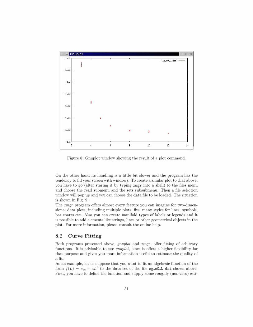
Figure 8: Gnuplot window showing the result of a plot command.

On the other hand its handling is a little bit slower and the program has thetendency to fill your screen with windows. To create a similar plot to that above,you have to go (after staring it by typing xmgr into a shell) to the files menuand choose the read submenu and the sets subsubmenu. Then a file selectionwindow will pop up and you can choose the data file to be loaded. The situationis shown in Fig. 9.The xmgr program offers almost every feature you can imagine for two-dimen-sional data plots, including multiple plots, fits, many styles for lines, symbols,bar charts etc. Also you can create manifold types of labels or legends and itis possible to add elements like strings, lines or other geometrical objects in theplot. For more information, please consult the online help.

8.2 Curve Fitting

Both programs presented above, gnuplot and xmgr , offer fitting of arbitraryfunctions. It is advisable to use gnuplot , since it offers a higher flexibility forthat purpose and gives you more information useful to estimate the quality ofa fit.As an example, let us suppose that you want to fit an algebraic function of theform f(L) = e∞ + aLb to the data set of the file sg e0 L.dat shown above.First, you have to define the function and supply some roughly (non-zero) esti-

51

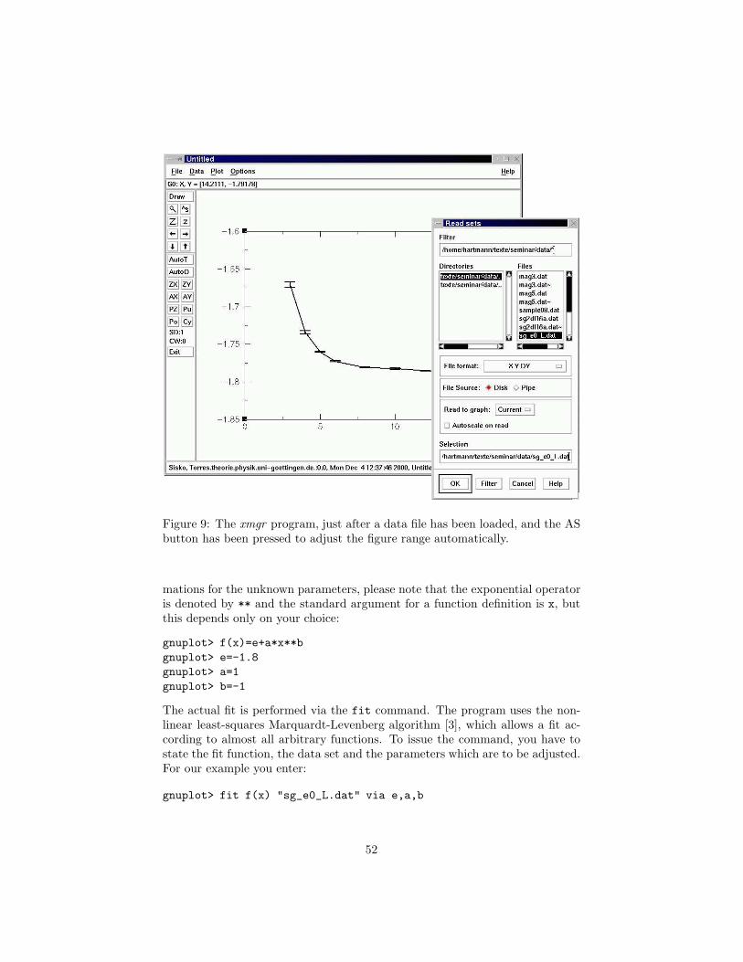
Figure 9: The xmgr program, just after a data file has been loaded, and the ASbutton has been pressed to adjust the figure range automatically.

mations for the unknown parameters, please note that the exponential operatoris denoted by ** and the standard argument for a function definition is x, butthis depends only on your choice:

gnuplot> f(x)=e+a*x**b

gnuplot> e=-1.8

gnuplot> a=1

gnuplot> b=-1

The actual fit is performed via the fit command. The program uses the non-linear least-squares Marquardt-Levenberg algorithm [3], which allows a fit ac-cording to almost all arbitrary functions. To issue the command, you have tostate the fit function, the data set and the parameters which are to be adjusted.For our example you enter:

gnuplot> fit f(x) "sg_e0_L.dat" via e,a,b

52

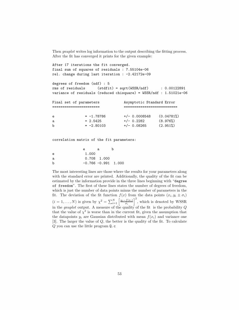
Then gnuplot writes log information to the output describing the fitting process.After the fit has converged it prints for the given example:

After 17 iterations the fit converged.

final sum of squares of residuals : 7.55104e-06

rel. change during last iteration : -2.42172e-09

degrees of freedom (ndf) : 5

rms of residuals (stdfit) = sqrt(WSSR/ndf) : 0.00122891

variance of residuals (reduced chisquare) = WSSR/ndf : 1.51021e-06

Final set of parameters Asymptotic Standard Error

======================= ==========================

e = -1.78786 +/- 0.0008548 (0.04781%)

a = 2.5425 +/- 0.2282 (8.976%)

b = -2.80103 +/- 0.08265 (2.951%)

correlation matrix of the fit parameters:

e a b

e 1.000

a 0.708 1.000

b -0.766 -0.991 1.000

The most interesting lines are those where the results for your parameters alongwith the standard error are printed. Additionally, the quality of the fit can beestimated by the information provide in the three lines beginning with “degreeof freedom”. The first of these lines states the number of degrees of freedom,which is just the number of data points minus the number of parameters in thefit. The deviation of the fit function f(x) from the data points (xi, yi ± σi)

(i = 1, . . . , N) is given by χ2 =∑N

i=1

[

yi−f(xi)σi

]2

, which is denoted by WSSR

in the gnuplot output. A measure of the quality of the fit is the probability Qthat the value of χ2 is worse than in the current fit, given the assumption thatthe datapoints yi are Gaussian distributed with mean f(xi) and variance one[3]. The larger the value of Q, the better is the quality of the fit. To calculateQ you can use the little program Q.c

53

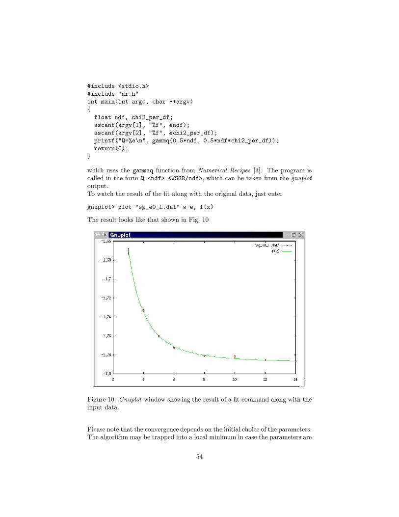
#include <stdio.h>

#include "nr.h"

int main(int argc, char **argv)

{

float ndf, chi2_per_df;

sscanf(argv[1], "%f", &ndf);

sscanf(argv[2], "%f", &chi2_per_df);

printf("Q=%e\n", gammq(0.5*ndf, 0.5*ndf*chi2_per_df));

return(0);

}

which uses the gammaq function from Numerical Recipes [3]. The program iscalled in the form Q <ndf> <WSSR/ndf>, which can be taken from the gnuplotoutput.To watch the result of the fit along with the original data, just enter

gnuplot> plot "sg_e0_L.dat" w e, f(x)

The result looks like that shown in Fig. 10

Figure 10: Gnuplot window showing the result of a fit command along with theinput data.

Please note that the convergence depends on the initial choice of the parameters.The algorithm may be trapped into a local minimum in case the parameters are

54

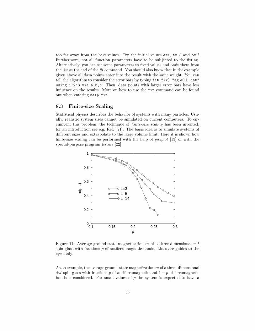
too far away from the best values. Try the initial values e=1, a=-3 and b=1!Furthermore, not all function parameters have to be subjected to the fitting.Alternatively, you can set some parameters to fixed values and omit them fromthe list at the end of the fit command. You should also know that in the examplegiven above all data points enter into the result with the same weight. You cantell the algorithm to consider the error bars by typing fit f(x) "sg e0 L.dat"

using 1:2:3 via a,b,c. Then, data points with larger error bars have lessinfluence on the results. More on how to use the fit command can be foundout when entering help fit.

8.3 Finite-size Scaling

Statistical physics describes the behavior of systems with many particles. Usu-ally, realistic system sizes cannot be simulated on current computers. To cir-cumvent this problem, the technique of finite-size scaling has been invented,for an introduction see e.g. Ref. [21]. The basic idea is to simulate systems ofdifferent sizes and extrapolate to the large volume limit. Here it is shown howfinite-size scaling can be performed with the help of gnuplot [13] or with thespecial-purpose program fsscale [22]

0.1 0.15 0.2 0.25 0.3p

0

0.2

0.4

0.6

0.8

1

m(p

,L)

L=3L=5L=14

Figure 11: Average ground-state magnetization m of a three-dimensional ±Jspin glass with fractions p of antiferromagnetic bonds. Lines are guides to theeyes only.

As an example, the average ground-state magnetization m of a three-dimensional±J spin glass with fractions p of antiferromagnetic and 1 − p of ferromagneticbonds is considered. For small values of p the system is expected to have a

55

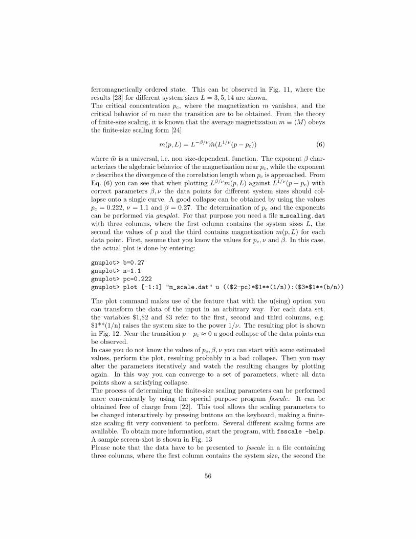
ferromagnetically ordered state. This can be observed in Fig. 11, where theresults [23] for different system sizes L = 3, 5, 14 are shown.The critical concentration pc, where the magnetization m vanishes, and thecritical behavior of m near the transition are to be obtained. From the theoryof finite-size scaling, it is known that the average magnetization m ≡ 〈M〉 obeysthe finite-size scaling form [24]

m(p, L) = L−β/νm(L1/ν(p − pc)) (6)

where m is a universal, i.e. non size-dependent, function. The exponent β char-acterizes the algebraic behavior of the magnetization near pc, while the exponentν describes the divergence of the correlation length when pc is approached. FromEq. (6) you can see that when plotting Lβ/νm(p, L) against L1/ν(p − pc) withcorrect parameters β, ν the data points for different system sizes should col-lapse onto a single curve. A good collapse can be obtained by using the valuespc = 0.222, ν = 1.1 and β = 0.27. The determination of pc and the exponentscan be performed via gnuplot . For that purpose you need a file m scaling.dat

with three columns, where the first column contains the system sizes L, thesecond the values of p and the third contains magnetization m(p, L) for eachdata point. First, assume that you know the values for pc, ν and β. In this case,the actual plot is done by entering:

gnuplot> b=0.27

gnuplot> n=1.1

gnuplot> pc=0.222

gnuplot> plot [-1:1] "m_scale.dat" u (($2-pc)*$1**(1/n)):($3*$1**(b/n))

The plot command makes use of the feature that with the u(sing) option youcan transform the data of the input in an arbitrary way. For each data set,the variables $1,$2 and $3 refer to the first, second and third columns, e.g.$1**(1/n) raises the system size to the power 1/ν. The resulting plot is shownin Fig. 12. Near the transition p− pc ≈ 0 a good collapse of the data points canbe observed.In case you do not know the values of pc, β, ν you can start with some estimatedvalues, perform the plot, resulting probably in a bad collapse. Then you mayalter the parameters iteratively and watch the resulting changes by plottingagain. In this way you can converge to a set of parameters, where all datapoints show a satisfying collapse.The process of determining the finite-size scaling parameters can be performedmore conveniently by using the special purpose program fsscale. It can beobtained free of charge from [22]. This tool allows the scaling parameters tobe changed interactively by pressing buttons on the keyboard, making a finite-size scaling fit very convenient to perform. Several different scaling forms areavailable. To obtain more information, start the program, with fsscale -help.A sample screen-shot is shown in Fig. 13Please note that the data have to be presented to fsscale in a file containingthree columns, where the first column contains the system size, the second the

56

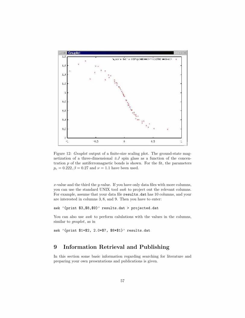
Figure 12: Gnuplot output of a finite-size scaling plot. The ground-state mag-netization of a three-dimensional ±J spin glass as a function of the concen-tration p of the antiferromagnetic bonds is shown. For the fit, the parameterspc = 0.222, β = 0.27 and ν = 1.1 have been used.

x-value and the third the y-value. If you have only data files with more columns,you can use the standard UNIX tool awk to project out the relevant columns.For example, assume that your data file results.dat has 10 columns, and yourare interested in columns 3, 8, and 9. Then you have to enter:

awk ’{print $3,$8,$9}’ results.dat > projected.dat

You can also use awk to perform calulations with the values in the columns,similar to gnuplot , as in

awk ’{print $1+$2, 2.0*$7, $8*$1}’ results.dat

9 Information Retrieval and Publishing

In this section some basic information regarding searching for literature andpreparing your own presentations and publications is given.

57

Figure 13: Screen-shot from a window running the fsscale tool.

9.1 Searching for Literature

Before contributing to the physical community and even publishing your results,you should be aware of what exists already. This prevents you from redoingsomething which has been done before by someone else. Furthermore, knowingprevious results and many simulation techniques allows you to conduct your ownresearch projects better. Unfortunately, much information cannot be foundin textbooks. Thus, you must start to look at the literature. With moderntechniques like CD-ROMs and the Internet this can be achieved very quickly.Within this section, it is assumed that you are familiar with the Internet andare able to use a browser. In the following list several sources of informationare contained.

• Your local (university) libraryAlthough the amount of literature is limited from space constraints, you

should always check your local library for suitable textbooks concerningyour area of research. Also many old issues of scientific journals are yet notavailable through the Internet, thus you may have to copy some articlesin the library.

58

• Literature databasesIn case you want to obtain all articles from a specific author or all ar-

ticles on a certain subject, you should consult a literature database. Inphysics the INSPEC [25] database is the appropriate source of informa-tion. Unfortunately, the access is not free of charge. But usually yourlibrary should allow access to INSPEC, either via CD-ROMS or via theInternet. If your library/university does not offer an access you shouldcomplain.

INSPEC frequently surveys almost all scientific journals in the areas ofphysics, electronics and computers. For each paper that appears, all bib-liographic information along with the abstract are stored. You can searchthe database for example for author names, keywords (in the abstract ortitle), publication years or journals. Via INSPEC it is possible to keeptrack of recent developments happening in a certain field.

There are many other specialized databases. You should consult the webpage of your library, to find out to which of them you can access. Mod-ern scientific work is not possible without regularly checking literaturedatabases.

• Preprint serverIn the time of the Internet, speed of publication becomes increasingly

important. Meanwhile, many researchers put their publications on the LosAlamos Preprint server [26], where they become available world wide atmost 72 (usually 24) hours after submission. The database is free of chargeand can be accessed from almost everywhere via a browser. The preprintdatabase is divided into several sections such as astrophysics (astro-ph),condensed matter (cond-mat) or quantum physics (quant-ph). Similar to aconventional literature database, you can search the database, eventuallyrestricted to a section, for author names, publication years or keywords inthe title/abstract. But furthermore, after you have found an interestingarticle, you can download it and print it immediately. File formats arepostscript and pdf. The submission can also be in TEX/LATEX (see Sec.9.2).

Please note that there is no editorial processing at all, that means youdo not have any guarantee on the quality of a paper. If you like, youcan submit a poem describing the beauty of your garden. Nevertheless,the aim of the server is to make important scientific results available veryquickly. Thus, before submitting an article, you should be sure that it iscorrect and interesting, otherwise you might get a poor reputation.

The preprint server also offers access via email. It is possible to subscribeto a certain subject. Then every working day you will receive a list of allnew papers which have been submitted. This is a very convenient wayof keeping track of recent developments. But be careful, not everyonesubmits to the preprint server. Hence, you still have to read scientificjournals regularly.

59

• Scientific journalsJournals are the most important resources of information in science. Mostof them allow access via the Internet, when your university or institutehas subscribed to them. Some of the most important physical journals,which are available online, are published by (in alphabetical order)

– the American Institute of Physics [27]

– the American Physical Society [28]

– Elsevier Science (Netherlands) [29]

– the European Physical Society [30]

– the Institute of Physics (Great Britain) [31]

– Springer Science (Germany) [32]

– Wiley-VCH (USA/Germany) [33]

– World-Scientific (Singapore) [34]

• Citation databasesIn every scientific paper some other articles are cited. Sometimes it is

interesting to get the reverse information, i.e. to obtain all papers whichare citing a given article A. This can be useful, if one wants to learn aboutthe most recent developments which are triggered by article A. In thatcase you have to access a citation index . For physics, probably the mostimportant is the Science Citation Index (SCI) which can be accessed viathe Web of Science [35]. You have to ask your system administrator oryour librarian whether and how you can access it from your site.

The American Physical Society (APS) [28] also includes links to citingarticles with the online versions of recent papers. If the citing article isavailable via the APS as well, you can immediately access the article fromthe Internet. This works not only for citing papers, but also for citedarticles.

• Phys NetIf you want to have access to the web pages of a certain physics depart-

ment, you should go via your web browser to the Phys Net pages [36].They offer a list of all physics departments in the world. Additionally,you will find lists of forthcoming conferences, job offers and many otheruseful links. Also, the home page of your department probably offers manyinteresting links to other web pages related to physics.

• Web browsingExcept for the sources mentioned so far, nowadays much information isavailable on net. Many researchers present their work, their results andtheir publications on their home pages. Quite often talks or computercodes can also be downloaded.

In case you cannot find a specific page through the Phys Net (see above), oryou are interested in obtaining all web pages concerning a specific subject,

60

you should ask a search engine. There are some very popular all purposeengines like Yahoo [37] or Alta Vista [38]. A very convenient way to starta query on several search engines in parallel is a meta search engine, e.g.Metacrawler [39]. To find out more, please contact a search engine.

9.2 Preparing Publications

In this section tools for two types of presenting your results are covered: via anarticle/report or in a talk. For writing papers, it is recommended that you useTEX/LATEX . Data plots can be produced using the programs explained in thelast section. For drawing figures and making transparencies, the program xfigoffers a large functionality. To create three-dimensional perspective images, theprogram Povray can be used. LATEX, xfig and Povray are introduced in thissection.First, TEX/LATEX is explained. It is a typesetting system rather than a wordprocessor. The basic program is TEX, LATEX is an extension to facilitate theapplication. In the area of theoretical computer science, the combination of TEXand LATEX is a widespread standard. When submitting an article electronicallyto a scientific journal usually LATEX has to be used. Unlike the conventional officepackages, with LATEX you do not see the text in the form it will be printed, i.e.LATEX is not a WYSIWYG (“What you see is what you get”) program. Thetext is entered in a conventional text editor (like Emacs) and all formattingis done via special commands. An introduction to the LATEX language can befound e.g. in Refs. [40, 41]. Although you have to learn several commands, theuse of LATEX has several advantages:

• The quality of the typesetting is excellent. It is much better than self-made formats. You do not have to care about the layout. But still, youare free to change everything according to your requirements.

• Large projects do not give rise to any problems, in contrast to manycommercial office programs. When treating a LATEX text, your computerwill never complain when your text is more than 300 pages or containsmany huge post-script figures.

• Type setting of formulae is very convenient and fast. You do not have tocare about sizes of indices of indices etc. Furthermore, in case you wantfor example to replace all α in your formulae with β, this can be donewith a conventional replace, by replacing all \alpha strings by a \beta

strings. For the case of an office system, please do not ask how to do thisconveniently.

• There are many additional packages for enhanced styles such as letters,transparencies or books. The bibtex package is very convenient, whichallows a nice literature database to be build up.

• Since you can use a conventional editor, the writing process is very fast.You do not have to wait for a huge packet to come up.

61

• On the other hand, if you still prefer a WYSIWYG (“what you see iswhat you get”) system, there is a program called lyx [42] which oper-ates like a conventional word processor but creates LATEX files as output.Nevertheless, once you get used to LATEX, you will never want to loose it.

Please note that this text was written entirely with LATEX. Since LATEX is a typesetting language, you have to compile your text to create the actual output.Now, an example is given of what a LATEX text looks like and how it can becompiled. This example will just give you an impression of how the systemoperates. For a complete reference, please consult the literature mentionedabove.The following file example.tex produces a text with different fonts and a for-mula:

\documentclass[12pt]{article}

\begin{document}

This is just a small sample text. You can write some words {\em

emphasized}\/, or in {\bf bold face}. Also different {\small sizes}

are possible.

An empty line generates a new paragraph. \LaTeX\ is very convenient

for writing formulae, e.g.

\begin{equation}

M_i(t) = \frac{1}{L^3} \int_V x_i \rho(\vec{x},t) d^3\vec{x}

\end{equation}

\end{document}

The first line introduces the type of the text (article, which is the standard)and the font size. You should note that all tex commands begin with a backslash(\), in case you want to write a backslash in your text, you have to enter$\backslash$. The actual text is written between the lines starting with

\begin{document} and ending with \end{document}. You can observe somecommands such as \em, \bf or \small. The { } braces are used to mark blocksof text. Mathematical formulae can be written e.g. with \begin{equation}and \end{equation}. For the mathematical mode a huge number of commandsexists. Here only examples for Greek letters (\alpha), subscripts (x i), fractions(\frac), integrals (\int) and vectors (\vec) are given.The text can be compiled by entering latex example.tex. This is the com-mand for UNIX, but LATEX exists for all operating systems. Please consult thedocumentation of your local installation.The output of the compiling process is the file example.dvi, where “dvi” means“device independent”. The .dvi file can be inspected on screen by a viewervia entering xdvi example.dvi or converted into a postscript file via typingdvips -o example.ps example.dvi and then transferred to a printer. Onmany systems it can be printed directly as well. The result will look like this:

This is just a small sample text. You can write some words empha-sized , or in bold face. Also different sizes are possible.

62

An empty line generates a new paragraph. LATEX is very convenientfor writing formulae, e.g.

Mi(t) =1

L3

∫

V

xiρ(~x, t)d3~x (7)

This example should be sufficient to give you an impression of what the phi-losophy of LATEX is. Comprehensive instructions are beyond the scope of thissection, please consult the literature [40, 41].Under UNIX/Linux, the spell checker ispell is available. It allows a simple spellcheck to be performed. The tool is built on a dictionary, i.e. a huge list ofknown words. The program scans any given text, also a special LATEX mode isavailable. Every time a word occurs, which is not contained in the list, ispellstops. Should similar words exist in the list, they are suggested. Now the userhas to decide whether the word should be replaced, changed, accepted or evenadded to the dictionary. The whole text is treated in this way. Please notethat many mistakes cannot be found in this way, especially when the misspelledword is equal to another word in the dictionary. However, at least ispell findsmany spelling mistakes quickly and conveniently, so you should use the tool.Most scientific texts do not only contain text, formulae and curves, but alsoschematic figures showing the models, algorithms or devices covered in the pub-lication. A very convenient but also simple tool to create such figures is xfig.It is a window based vector-oriented drawing program. Among its features arethe creation of simple objects like lines, arrows, polylines, splines, arcs as wellas rectangles, circles and other closed, possibly filled, areas. Furthermore youcan create text or include arbitrary (eps, jpg) pictures files. You may place theobjects on different layers which allows complex sceneries to be created. Differ-ent simple objects can be combined into more complex objects. For editing youcan move, copy, delete, rotate or scale objects. To give you an impression whatxfig looks like, in Fig. 14 a screen-shot is shown, displaying xfig with the picturethat is shown in Fig. 1. Again, for further help, please consult the online helpfunction or the man pages.The figures can be saved in the internal fig format, and exported in several fileformats such as (encapsulated) postscript , LATEX, Jpeg, Tiff or bitmap. Thexfig program can be called in a way that it produces just an output file witha given fig input file. This is very convenient when you have larger projectswhere some small picture objects are contained in other pictures and you wantto change the appearance of the small objects in all other files. With the helpof the make program pretty large projects can be realized.Also, xfig is very convenient when creating transparencies for talks, which isthe standard method of presenting results in physics. With different colors,text sizes and all the objects mentioned before, very clear transparencies canbe created quickly. The possibility of including picture files, like postscript fileswhich were created by a data plotting program such as xmgr , is very helpful.In the beginning it may seem that more effort is necessary than when creatingthe transparencies by hand. However, once you have a solid base of transparen-cies you can reuse many parts and preparing a talk may become a question of

63

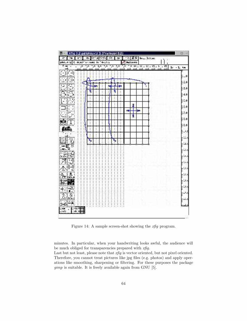
Figure 14: A sample screen-shot showing the xfig program.

minutes. In particular, when your handwriting looks awful, the audience willbe much obliged for transparencies prepared with xfig.Last but not least, please note that xfig is vector oriented, but not pixel oriented.Therefore, you cannot treat pictures like jpg files (e.g. photos) and apply oper-ations like smoothing, sharpening or filtering. For these purposes the packagegimp is suitable. It is freely available again from GNU [5].

64

It is also possible to draw three-dimensional figures with xfig, but there is nospecial support for it. This means, xfig has only a two-dimensional coordinatesystem. A very convenient and powerful tool for making three-dimensionalfigures is Povray (Persistence Of Vision RAYtraycer). Here, again, only a shortexample is given, for a detailed documentation please refer to the home page[43], where the program can be downloaded for many operating systems free ofcharge.Povray is, as can be realized from its name, a raytracer . This means youpresent a scene consisting of several objects to the program. These objects havecharacteristics like color, reflectivity or transparency. Furthermore the positionof one or several light sources and a virtual camera have to be defined. Theoutput of a raytracer is a photo-realistic picture of the scene, seen through thecamera. The name “raytracer” originates from the fact that the program createsa picture by starting several rays of light at the light sources and traces theirway through the scene, where they may be absorbed, reflected or refracted,until they hit the camera, disappear into infinity or become too weak. Hence,the creation of a picture may take a while, depending on the complexity of thescene.A scene is described in a human readable file, it can be entered with any texteditor. But for more complex scenes, special editors exist, which allow a scene tobe created interactively. Also several tools for making animations are availableon the Internet. Here, a simple example is given. The scene consists of threespheres connected by two cylinders, forming a molecule. Furthermore, a lightsource, a camera, an infinite plane and the background color are defined. Pleasenote that a sphere is defined by its center and a radius and a cylinder by twoend points and a radius. Additionally, for all objects color information has tobe included, the center sphere is slightly transparent. The scene description filetest1.pov reads as follows:

#include "colors.inc"

background { color White }

sphere { <10, 2, 0>, 2

pigment { Blue } }

cylinder { <10, 2, 0>, <0, 2, 10>, 0.7

pigment { color Red } }

sphere { <0, 2, 10>, 4

pigment { Green transmit 0.4} }

cylinder { <0, 2, 10>, <-10, 2, 0>, 0.7

pigment { Red } }

sphere { <-10, 2, 0>, 2

65

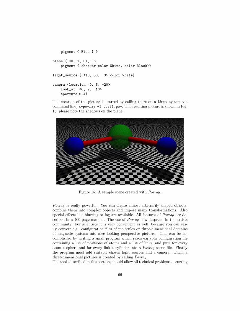
pigment { Blue } }

plane { <0, 1, 0>, -5

pigment { checker color White, color Black}}

light_source { <10, 30, -3> color White}

camera {location <0, 8, -20>

look_at <0, 2, 10>

aperture 0.4}

The creation of the picture is started by calling (here on a Linux system viacommand line) x-povray +I test1.pov. The resulting picture is shown in Fig.15, please note the shadows on the plane.

Figure 15: A sample scene created with Povray.

Povray is really powerful. You can create almost arbitrarily shaped objects,combine them into complex objects and impose many transformations. Alsospecial effects like blurring or fog are available. All features of Povray are de-scribed in a 400 page manual. The use of Povray is widespread in the artistscommunity. For scientists it is very convenient as well, because you can eas-ily convert e.g. configuration files of molecules or three-dimensional domainsof magnetic systems into nice looking perspective pictures. This can be ac-complished by writing a small program which reads e.g your configuration filecontaining a list of positions of atoms and a list of links, and puts for everyatom a sphere and for every link a cylinder into a Povray scene file. Finallythe program must add suitable chosen light sources and a camera. Then, athree-dimensional pictures is created by calling Povray.The tools described in this section, should allow all technical problems occurring

66

in the process of preparing a publication (a “paper”) to be solved. Once youhave prepared it, you should give it to at least one other person, who should readit carefully. Probably he/she will find some errors or indicate passages whichmight be difficult to understand or that are misleading. You should alwaystake such comments very seriously, because the average reader knows much lessabout your problem than you do.After all necessary changes have been performed, and you and other readersare satisfied with the publication, you can submit it to a scientific journal. Youshould choose a journal which suits your paper. Where to submit, you shoulddiscuss with experienced researchers. It is not possible to give general advice onthis issue. Nevertheless, technically the submission can be performed nowadaysalmost everywhere electronically. For a list of publishers of some importantjournals in physics, please see Sec. 9.1. Submitting one paper to several journalsin parallel is not allowed. However, you should also consider submitting to thepreprint server [25] as well to make your results quickly available to the physicscommunity.Nevertheless, although this text provides many useful hints concerning perform-ing computer simulations, the main part of the work is still having good ideasand carefully conducting the actual research projects.

References

[1] I. Sommerville, Software Engineering, (Addisin-Wesley, Reading (MA)1989)

[2] C. Ghezzi, M. Jazayeri, and D. Mandrioli, Fundamentals of Software En-gineering, (Prentice Hall, London 1991)

[3] W.H. Press, S.A. Teukolsky, W.T. Vetterling, and B.P. Flannery, NumericalRecipes in C (Cambridge University Press, Cambridge 1995)

[4] K. Mehlhorn and St. Naher, The LEDA Platform of Combinatorial andGeometric Computing (Cambridge University Press, Cambridge 1999);see also http://www.mpi-sb.mpg.de/LEDA/leda.html

[5] M. Loukides and A. Oram, Programming with GNU Software, (O’Reilly,London 1996);see also http://www.gnu.org/manual

[6] H.R. Lewis and C.H. Papadimitriou, Elements of the Theory of Computa-tion, (Prentice Hall, London 1981)

[7] J. Rumbaugh, M. Blaha, W. Premerlani, F. Eddy, and W. Lorensen, Object-Oriented Modeling and Design, (Prentice Hall, London 1991)

[8] R. Johnsonbaugh and M. Kalin, Object Oriented Programming in C++,(Macmillan, London 1994)

67

[9] J. Skansholm, C++ from the Beginning, (Addisin-Wesley, Reading (MA)1997)

[10] Mail to [email protected]

[11] B.W. Kernighan and D.M. Ritchie, The C Programming Language, (Pren-tice Hall, London 1988)

[12] A. Oram and S. Talbott, Managing Projects With Make, (O’Reilly, London1991)

[13] The programs and manuals can be found on http://www.gnu.org. For somethere is a texinfo file. To read it, call the editor ’emacs’ and type <crtl>+’h’and then ’i’ to start the texinfo mode.

[14] J. Phillips, The Nag Library: A Beginner’s Guide (Oxford University Press,Oxford 1987);see also http://www.nag.com

[15] A. Heck, Introduction to Maple, (Springer-Verlag, New York 1996)

[16] B.J.T. Morgan, Elements of Simulation, (Cambridge University Press,Cambridge 1984)

[17] A.M. Ferrenberg, D.P. Landau and Y.J. Wong, Phys. Rev. Lett. 69, 3382(1992); I. Vattulainen, T. Ala-Nissila and K. Kankaala, Phys. Rev. Lett.73, 2513 (1994)

[18] J.F. Fernandez and C. Criado, Phys. Rev. E 60, 3361 (1999)

[19] http://www.cs.colorado.edu/homes/zorn/public html/MallocDebug.html

[20] The tool can be obtained under the gnu public license fromhttp://www.gnu.org/software/checker/checker.html

[21] J. Cardy, Scaling and Renormalization in Statistical Physics , (CambridgeUniversity Press, Cambridge 1996)

[22] The program fsscale is written by A. Hucht, please contact him via email:[email protected]

[23] A.K. Hartmann, Phys. Rev. B 59 , 3617 (1999)

[24] K. Binder and D.W. Heermann, Monte Carlo Simulations in StatisticalPhysics , (Springer, Heidelberg 1988)

[25] http://www.inspec.org/publish/inspec/

[26] http://xxx.lanl.gov/

[27] http://www.aip.org/ojs/service.html

68

[28] http://publish.aps.org/

[29] http://www.elsevier.nl

[30] http://www.eps.org/publications.html

[31] http://www.iop.org/Journals/

[32] http://www.springer.de/

[33] http://www.wiley-vch.de/journals/index.html

[34] http://ejournals.wspc.com.sg/journals.html

[35] http://wos.isiglobalnet.com/

[36] http://physnet.uni-oldenburg.de/PhysNet/physnet.html

[37] http://www.yahoo.com/

[38] http://www.altavista.com/

[39] http://www.metacrawler.com/index.html

[40] L. Lamport and D. Bibby, LaTeX : A Documentation Preparation Sys-tem User’s Guide and Reference Manual , (Addison Wesley, Reading (MA)1994)

[41] http://www.tug.org/

[42] http://www.lyx.org/

[43] http://www.povray.org/

69

Documents

A Practical Guide to Computer Simulations