1

A practical designer’s guide to mesozooplankton nets Eric Keen

January 2013

1. Introduction 2. Theoretical Framework 2.1 Starting Points 2.2 The Open-Area Ratio 2.3 Initial Filtration Efficiency (IFE) 2.3.1 Net shape 2.3.2 OAR 2.3.3 Tow Speed 2.3.4 Washing & Care 2.4 Sustained Filtration Efficiency (SFE) 2.4.1 Mesh Size 2.4.2 OAR Revisited 3. Approach 3.1 Net Model 3.1.1 Geometry 3.1.2 IFE 3.1.3 Geometric Relationships 3.2 Case Study 4. Choosing a Net 4.1 Step 1: First Steps 4.2 Step 2: Mesh Size 4.2.1 Porosity 4.3 Step 3: Diameter 4.4 Step 4: Tow Duration 4.4.1 Constraints 4.4.1.1 From Sampling Design 4.4.1.2 From the Literature 4.4.1.3 Imposed by Study Area 4.4.2 Practical Proxies for Tow Volume 4.4.3 Results 4.5 Step 5: Minimum Open-Area Ratio 4.5.1 Green vs. Blue Waters 4.5.2 Results 4.6 Step 6: Solving for Net Length 5. Concluding Remarks Appendix 1: Case study Appendix 2: Taking our results “shopping” Appendix 3: Adding a strobe light? Literature Cited Figures & Tables

  2

1. Introduction

While in the field and during data analysis, a poorly chosen net leads to problems that can prove fatal to a plankton study. Net clogging, inefficient use of ship time, unnecessary use of deck space, the extrusion, escape or avoidance of target species, the exhaustion of crew working the net, insufficient sample size, and the collection of hollow data unable to speak to the stated hypotheses are some examples of problems that can befall studies if net choice is not taken seriously. The ordeal of choosing an appropriate net begins with the same concerns fundamental to any field-based research: 1) the objectives of your study; 2) the conditions of your study area; and 3) the resources that are available to you. These three considerations must be weighed in careful compromise in order to arrive at an appropriate configuration with confidence. Finding that optimal compromise and then setting out to obtain a net can be daunting tasks. This guide is intended to help researchers leverage their constraints as tools in a decision-making process. After a brief foundation in the conceptual framework underpinning appropriate net design, an investigator can make a series of decisions that begins at the basic facts regarding her planned study and leads to a firm grasp of the best net for the job. Readers may not only identify the optimal combination of net parameters, but can also define a range of options from which to choose, offering them further agency when it comes time to buy, build or rent their net. Our discussion will rely on a design of cylindrical-conical (cyl-cone) net similar to the WP-2 standard (Figure 1), named after Working Party no. 2, the team of scientists who designed the net in an attempt to standardize field equipment and best practices for a specific size class of organisms (Tranter & Fraser 1968). The WP-2 net is “a standard sampler of simple, practicable design…for quantitative, comparative biomass studies of marine plankton in the upper 200m of water…in the size spectrum from 10mm downward to a width of at least 200µ.” While their schematic is not ideal in many circumstances, most studies have used “cyl-cone” samplers in the vein of the WP-2 design ever since. The approach we offer here is a synthesis of many studies from a long history of field planktology (reviewed in Wiebe et al. 2003), but four landmark papers stand out: Tranter & Smith (1968), Harris et al. (2000, esp. chapters 2 and 3), Bernardi (1984), and, most recently, Ohman (2013). These in particular give readers a newfound respect for such questions as seemingly simple as, “Which net should I use?” They also provide excellent guidance in sampling design and organism preservation. However, upon finishing these papers readers might feel more daunted than empowered, more helpless than helped, and still not sure where to begin. Understandably, given their broad coverage of topics for a wide range of organisms, these papers are unable to offer much specific, concrete advice regarding net design. (For other aspects of sampling, however, they are highly practical). Here we err on the other side of the compromise, by attempting to provide specific, step-by-step instructions in net design at the cost of a substantially limited scope. This manual is for studies of pelagic mesozooplankton that involve single- or dual-net samplers for mesozooplankton. As such, it is most readily helpful to small-scale, low-budget

  3

studies conducted by single researchers or small teams. However, the lower frequencies of our approach should be applicable to a variety of other purposes, from benthic trawls to multi-net samplers (e.g. MOCNESS) to high-speed samplers to studies of phytoplankton or fish. Our scope is further limited to the selection of three key net parameters: diameter of the net’s mouth, overall net length, and aperture of the mesh material (i.e., mesh size). These combine to influence a net’s filtration efficiency and a net’s propensity to clog. These “key three” are also the most readily observable when looking at a candidate net, so it is convenient that the decision process is centered upon their interaction. While a net has many other parameters that can increase its efficacy (e.g., net color, bridle and flowmeter rigging, etc.), the key three are all that one needs to get started.

2. Theoretical Framework 2.1 Starting Points A good net must perform well and consistently in the following ways:

1. Retain the organisms targeted by the study’s objectives, minimizing their ability to avoid the net and escape through the mesh.

2. Filter a sufficient volume of water over sufficient depths to provide statistically robust results.

3. Sample for said duration before clogging significantly deteriorates filtration efficiency and the size selectivity of the mesh.

4. Be sustainably operable given the finite energies of the crew and resources at your disposal.

Because all of these functions are critical if the study is to be worthwhile, it is difficult to know where to begin. We move forward using the following rationale: Concerns of operability (criterion #4) -- including net drag, pay-out and retrieval methods, towing speed and depth, and the strength of rigging and crew -- are pointless if the operation is futile to begin with. While such logistics will come into play throughout the decision process, they won’t govern its overall trajectory. If, however, a net suffers from a poor filtration efficiency to begin with and clogs easily (#3), it will fail at both capturing target organisms (#1) and filtering sufficient volumes of water (#2) at a sustained efficacy. Therefore, the imperative upon which all other criteria hinge, and the concern that will organize and motivate the decision tree we outline below, is the need to maximize and maintain a net’s filtration efficiency. Filtration efficiency is the percent of water a net passes through that is actually sampled. As we will see, net performance can be discussed in terms of both initial and sustained filtration efficiency (IFE and SFE, respectively). (Tranter & Smith 1968 abbreviated filtration efficiency as F. In an effort to emphasize the distinction between initial and sustained efficiency, we use a different notation here.) In addition to impacting the volume of each tow, clogging over the course of a tow can cause the net to become increasingly size selective, introducing a host of biases to results. Filtration efficiency can also affect rates of net avoidance and escapement. See Tranter & Smith (1968) for an excellent review.

  4

2.2 The Open Area Ratio The primary objective in net design is twofold: 1) maximize initial filtration efficiency of the net, then 2) sustain that efficiency for as long a tow as possible. The “open-area ratio”, OAR, is a useful metric that plays a role in both directives. OAR is the ratio of the filtering mesh area to the area of the net’s mouth opening. (Note: in Tranter & Fraser 1968 and other early works, the open-area ratio is abbreviated simply as R. Here, we follow Ohman 2013).

OAR= filtering area/mouth area = β*a /A

β = porosity a = total area of net A= mouth area

The “filtering mesh area” refers to the total open area of the net’s mesh, which can be found by multiplying the net’s surface area by the mesh’s “porosity”, or percent open area. A net’s surface area can be calculated using the geometry of the net’s shape, total net length and mouth diameter. Mouth diameter also determines the area of the mouth opening, meaning it influences both sides of the open-area ratio. Hence our “key three” combine to determine our net’s OAR, the defining metric of filtration performance. The OAR of a net plays a complimentary role in initial filtration efficiency, but a defining role in sustaining that efficiency over the course of a tow. In general, the higher the OAR ratio of a net, the better for both IFE and SFE. The rub, however, is that other concerns constrain the design of our net, and a sufficient OAR can sometimes be difficult to attain. Net selection is therefore a game of trade-offs, driven by the conflicting priorities of maximizing OAR, maximizing sample size, and minimizing cost and effort. 2.3 Initial Filtration Efficiency (IFE) The style and geometry of a net largely determine a net’s IFE, but there are some configurations for which OAR, tow speed, and the initial cleanliness of the mesh also play a determining role. Generally speaking, a higher IFE means better use of sampling effort and more flexibility in the design steps later on. IFE values for conventional net types range from 75% (simple conical nets) to upwards of 110% (reducing collar cyl-cone nets). The WP-2 has an IFE of 94% (Tranter & Fraser 1968). Some are motivated to maximize this parameter into the realm of 110-120%, while others design for 100% IFE to simplify calculations (Tranter & Smith 1968). 2.3.1 Net Shape The geometry of a net governs the way in which water flows through and around it. The hydrodynamics of this flow are sensitive to a slew of variables, which are reviewed at length in Tranter & Smith (1968). Here it suffices to summarize their main points:

- Nets without nonporous encasements are more efficient than those with (Figure 2). - Simple conical nets are among the least efficient, at about 75-85%. - IFE declines sharply when the net’s side angle (Θ in Figure 3), the angle of incidence

of water striking the mesh, falls below 75° (or when the ratio A/a rises above 0.2).

  5

- IFE increases significantly when a porous cylindrical section of mesh is added ahead of the cone; such cyl-cone nets have been found to have some of the highest IFE’s of any design (Smith, Counts, and Clutter 1968). There are two supposed reasons for this boost: 1) water rejected by the tapering area of the cone will escape through the cylinder’s mesh (Currie 1963); and 2) cylindrical collars tend to oscillate under tow, “possibly in response to eddies shed by the ring, and so cleans itself of accumulated organisms” (Tranter & Smith 1968).

- A cylindrical section also adds more filtering area while adding less to the overall length of the net than a conical form would; put another way, a cylindrical-conical net has a higher OAR than a conical net of the same overall length.

- By adding filtering area and thus increasing OAR, a cylindrical section also ameliorates sustained filtering efficiency, increasing the duration that a net can tow before clogging.

- Enlarging the terminal radius of the cylindrical section to create a “mouth reducing cone” (Figure 2c) increases IFE, enabling levels of 110% or more. In addition to increasing OAR, this reducing cone creates a low pressure area within the net at the terminus of the cylindrical section, which sucks in a column of water wider than the mouth (Tranter & Smith 1968).

- Such reducing cones are more efficient when their angle of expansion is small (Tranter & Heron 1967). For top efficiency, the angle should be less than 3.5° (Pankhurst and Holder 1952). This is achieved by either keeping the discrepancy between the two radii of the cylindrical section small, or, preferably, by lengthening the cylindrical section.

2.3.2 OAR As outlined above, the boosted IFE of a cyl-cone net can be explained by both mechanical effects (e.g. self-cleansing) and the enlarged OAR that comes with the addition of filtering area. However, improving OAR only boosts IFE up to a certain point; the effect plateaus above an OAR of 3. Tranter & Smith (1968) assert that to achieve an IFE of 85%, a minimum OAR of 3 is required; for 95%, the OAR should be 5, but anything higher is not likely to have a significant impact. Their rationale for this diminishing return involves hydrodynamic theory. As we will see, OAR (along with the net features implicated in it: mouth diameter, mesh size, and overall length) becomes much more influential in matters of sustained filtering efficiency. 2.3.3 Tow Speed Nets towed at very low speed (< .5 m/s, or 1 knot) filter at a lower efficiency (Tranter & Smith 1968). Again, however, the effect plateaus; at speeds greater than 0.5m/s, IFE is unaffected. From the literature review conducted for our case study (see below), most tow speeds were between 1.5 knots (.77 m/s, Fiedler et al. 1998) to 2.5 knots (1.28 m/s, Mackas & Galbraith 2002, Schulenberger 1978). The median tow speed reported was 2 knots, or ~1 m/s. In an effort to standardize methods, Working Party No. 2 recommended that vertical tows – which are typically slower than oblique hauls -- be raised at 0.75m/s (Tranter & Fraser 1968). Higher tow speeds (> 1.5 m/s) may allow for shorter tow durations and may or may not minimize avoidance (Clutter & Anraku 1968), but they will probably damage specimens. This is not caused by the speed itself, but by the pressure drop across the mesh. Investigators wishing to collect specimens for live experiments or precise morphological

  6

studies must prioritize minimal tow speed. Furthermore, the towing cable or deck rigging for the cable can also become strained at high speeds, and manual retrieval of the net is very tiresome at anything above idle speed. Samplers specifically designed for high tow speeds, such as continuous plankton recorders, are beyond the scope of this paper. 2.3.4 Washing & Care Plankton dry more completely on monofilament nylon mesh (which has now become the industry standard) compared to older silk designs. The presence of remnant plankters and debris in successive tows can introduce variable IFEs over the course of a study (Tranter & Smith 1968). Thorough rinsing between tows with uncontaminated fresh water is critical to maintaining consistent OAR and IFE values (see Harris et al. 2000 for best practices in net care and storage). 2.4 Sustained Filtration Efficiency (SFE) Over the course of a tow, clogging will cause the net’s filtration efficiency to deteriorate. Detritus, suspended “snow” particles, phytoplankton, and the target organisms themselves can have a nefarious impact on zooplankton studies. Clogging introduces more and more bias over the course of a tow, not only by reducing overall filtration efficiency, but by selectively sampling a progressively constrained size range of organisms (Ohman 2013). When testing the performance of a net, clogging can be monitored by comparing readings from two flowmeters, one mounted inside and the other outside of the net (Tranter & Smith 1968). The rate at which clogging occurs is a function of the conditions of the study area, over which we have little control, and the design of our net. By convention, once filtration efficiency has dropped below 85% of initial, the net has ceased to perform effectively (Smiths, Counts & Clutter 1968). Sampling enough water before this occurs is the central goal. Open-area ratio, mesh size, and, to a lesser extent, net shape governs SFE. As explained above, the geometry of a net can introduce “self-cleaning” behaviors that increase the duration of efficient filtration. A cylindrical or mouth-reducing section can also add filtering area to the net, increasing the OAR. 2.4.1 Mesh Size The width of holes in mesh influence SFE in two ways. First, fine gauze will clog more readily than coarse gauze merely because it catches more particles. In fact, the effective tow duration of a net declines as a function of the square of the mesh width (Smith, Counts & Clutter 1968). In order to compensate for the inherently low SFE of fine mesh nets, OAR must dramatically increase. For mesh widths greater than 300µ, Tranter & Smith (1968) recommend an overall OAR of 5 or higher, with an OAR of 3 in the conical portion and an OAR of 2 in the cylinder. They warn that any mesh smaller than that would require an OAR of 9 or higher, with 3 in the cone and 6 in the cylinder. However, in the same monograph, Working Party 2 proposed a standardized net schematic with 200µ mesh that had an OAR of only 6:1, 3 in the cylinder and 3 in the cone (Tranter & Fraser 1968). To err on the conservative side (sensu Ohman 2013), we will hold minimum OAR at 9:1 for mesh

  7

apertures less than 300µ. But Working Party No. 2 makes the good point that such arbitrary thresholds should be taken merely as guidelines. Second, mesh size determines a net’s porosity, a term in the OAR equation. While one would expect porosity to decrease linearly with shrinking mesh size, different widths of Nylon monofilament are used in weaves for various mesh sizes, such that porosity levels rise and fall abruptly as mesh size increases. We were able to find two distributors that reported porosities for the Nitex mesh they sell, Wildlife Supply Company (WSC)1 and Dynamic-Aqua Supply, Ltd. (DAS)2. Since mesh of the same aperture can be available at different porosities (Figure 4), seeking out the most porous mesh available will help to maximize your net’s OAR, and may allow you to get away with a shorter net.3 While high-porosity material may not be as supple as thick-filament, low porosity mesh, weave strength is not of great concern for small-scale studies with low tow speeds. 2.4.2 OAR Revisited Controlling for the size and abundance of particles in the water, the open-area ratio indicates the duration of filtration that is possible before clogging sets in. A slight change in OAR can have major effects on the effective duration of a tow; Smith, Counts and Clutter (1968) found that a doubling in OAR from 3.2 to 6.4 increased the volume filtered efficiently by sixfold. The OAR of a net is a compromise between porosity, filtering area, and mouth area – which are products of a net’s mesh size, diameter, and overall length – all of which are constrained by the organisms of interest, target volume, and resources. As such, the OAR represents a game of trade-offs. Here is the OAR equation, repeated for convenience:

OAR= β *a/A All else being held constant, lengthening a net will increase its OAR, as will choosing a mesh size that is more porous. Note that since diameter is implicated in both the numerator and denominator of the OAR equation – both of which involve exponents -- the nature of its impact on OAR is depends on the net size in question. Generally speaking, however, the largest OARs are achieved with the longest total length, smallest mouth openings, and most porous mesh. Conversely, the smallest OARs occur in the shortest nets with large mouth openings and low-porosity gauze.

3. Approach The framework above leaves us with some minimum standards our net. First, the effort to maximize initial filtration efficiency constrains some ancillary variables: tow speed must be above 0.5 m/s; the net should have a fore cylindrical section or mouth-reducing cone; the                                                                                                                1 www.wildco.com 2 http://www.dynamicaqua.com/nitex.html 3 Mesh aperture and porosity can be difficult to know if a net does not come with documentation. Smith, Counts, & Clutter (1968) provide instruction on measuring and calculating these values using a microscope.

  8

minimum acceptable OAR is 3. If mesh size is less than 300 microns, this minimum OAR increases to 9 (Tranter & Smith 1968). Within these constraints, we can approach the questions of diameter, mesh size, and overall length using quantitative models. Sustaining this filtration efficiency, however, presents another procedural puzzle: The interaction of the “key three” parameters is such that several different configurations can result in the same OAR. Moreover, these parameters are dynamically coupled (e.g. diameter affects both filtering area and mouth area). Which parameters should we constrain first, and how do we make that decision? This is our basis for a way forward (visualized in Figure 5): The primary motivator of any research initiative is its central questions; without them, there would be no initiative at all. And, in one form or another, all zooplanktoon studies set out to gather data on a specific taxon, group of taxa, or groups within a taxon (e.g., life stages), within a specified study area. Therefore, we ought to identify target organisms first. Using biometric and behavioral knowledge of those target taxa, we can constrain mesh size and net diameter. Next, with knowledge about the habitat preferences of target taxa and the conditions in our study area, we arrive at a sampling plan with target volumes for every tow. What remains is achieving an OAR that makes that sampling plan feasible without recourse to modifying mesh size or diameter. To do so we must rely, finally, on adjusting the overall length of the net. There are certainly reasons to minimize the length of the net, including the high cost of mesh yardage, the loss of deck space, and the difficulties of handling the drag. However, while limited resources are an important consideration for any study, it is better to purchase a net that is expensive and cumbersome -- but appropriate -- than one that is cheap, easy to handle, but scientifically useless. Concerns of length must give privy to those of mesh size and diameter, since the latter stem directly from the basal objectives of the study. In the end, our mesh size will be constrained by target organisms, our diameter will be constrained by both target organisms and our resources, and the minimum OAR of our net will be determined by our mesh size, desired sampling volume, and the conditions of the study area. The one parameter that remains variable is overall net length, and it must be adjusted last to accommodate the others. Below we present a step-by-step walk through of the design process. Each decision informs those in the subsequent step. It will lead to an optimal combination of the “key three” parameters (diameter, length, and mesh size). The figures associated with each step provide a convenient visual means of constraining parameters. Note that some figures are specific to the type of tow intended (vertical or horizontal/oblique). 3.1 Net Model 3.1.1 Geometry The net type and geometry used in the calculations throughout is a simplistic adaptation of WP-2 cyl-cone design (Figure 3). Conical nets have a lower IFE, generally requiring a higher OAR to sample the same volume of water as efficiently as a cylindrical-conical net of the same length. Mouths with reducing cones have a higher IFE, but they are less

  9

commonly available, and because our goal here is to determine minimum requirements, using a cyl-cone net is most prudent. Because all nets reduce not to a point but to a terminal cod-end bucket, the “cones” of nets are actually tapered cylinders. The mean cod-end diameter of 63 nets sampled from the Scripps Institution of Oceanography Pelagic Invertebrate Collection (SIO PIC) was 10.95cm (see Appendix 2). A cod-end of 7.5cm diameter was recommended by the Working Party No. 2 (1968), which is a value within the standard deviation of the PIC sample (sd=4.2cm). A diameter of 7.5cm therefore provides a standard value that ensures we will err on the side of underestimating OAR. 3.1.2 IFE To maximize IFE, we will only consider configurations that yield an OAR greater than 3. As we manipulate net length relative to diameter, we will not allow the side angle of the net to fall below 75° (which would decrease IFE); in other words, for a given diameter, there is a certain minimum length the net must be. The tow speed we use in calculations of tow duration will not fall below 0.5 m/s nor exceed 1.5 m/s, and the average will be 1 m/s (2 knots). The average IFE for conventional cyl-cone net configurations reported by Tranter & Smith (1968, Table 5, n=7) was 94.43% ±2.99%. To remain conservative, our model’s configuration will have an IFE one standard deviation below that mean, at 91.4%. 3.1.3 Geometric Relationships The parameters used to calculate the geometric net configurations below are summarized in Table 1. Because the cylindrical section adds the most OAR to a net with a comparatively minor addition of total length, the conical section’s length will be minimized. The strict minimum of the side angle (Θ) is 75° (Tranter & Smith 1968), but we will keep our model’s at the side angle used in the WP2 net, 81.33°. With this angle immobilized, we can calculate the length of the conical section (lcone) of any net by knowing only the radii of its mouth (R) and its cod-end (r, given above as 3.5cm).

lcone = tanΘ * (R – r) The length of the cylindrical section will comprise the remainder of the net’s overall length. This means that low OAR nets will have proportionally longer conical sections than those with a high OAR. In nets with an OAR of 10 or higher, the majority of its length will be composed of cylindrical section. In fact, the length ratio of the cylindrical and conical sections may swing from 2:3 to 6:3 as net length increases (Smith & Clutter 1965, Tranter & Smith 1968). The overall length of the net (ltotal) will be the simple sum of the lengths of the cylindrical and conical sections (lcyl and lcone, respectively).

ltotal = lcone + lcyl

  10

Similarly, the total filtering area of the net (a) will be the sum of the lateral surface areas of each section (acyl and acone).

a = acyl + acone Using conventional geometric equations, these surface areas are calculated as follows:

acyl = 2*pi*lcyl acone = pi*(R + r)*s

Where s is the side length of the conical section of net, which can be thought of the hypotenuse of a right triangle with side lengths lcone and R – r. As such, the classic Pythagorean relationship applies:

s = √(lcone2 + (R – r)2) These equations will be used to calculate overall net length, which shall be the last variable standing after diameter, mesh size (= porosity) and OAR are constrained. To verify that the above equations yield accurate results, we used the WP2 schematic provided in Tranter & Fraser (1968) as a check (Figure 1). The schematic provides us with 200µ mesh aperture, 0.57m diameter, .95m cylinder length, 1.66m side length (different from cone length), and an OAR of 6:1. The porosity for this mesh size is reported as 45% by Dynamic Aqua Ltd. (Figure 4; the same value is given in Table 4 in Tranter & Smith 1968). By assuming this net has a 0.075m diameter cod-end, we can use simple right-angle geometry to calculate the cone’s side angle (81.33°) and the length of the cone (1.64m), which tells us the WP2’s total length is the sum of its two section lengths, 2.59m. Using just mesh size, diameter, and OAR from the WP2 schematic (as well as given values for cod-end diameter and side angle), we predicted that the overall length of the net would be 2.566m, with 0.961m in the cylinder and 1.604m in the cone. These values are with 2% of the actual dimensions. 3.2 Case Study To illustrate each step of the decision making process, we use a case study set in the northern fjords of British Columbia, Canada. See Appendix 1 for a full description of this case study and an application of the procedure we outline below. The primary objective of this study is to document trophic interactions between rorqual whales and their prey. Primary target species include locally dominant euphausiids and large-bodied copepods.

  11

4. Choosing a net 4.1 Step 1: First Steps Determining the right net for your study first requires that you rigorously define the study’s objectives and familiarize yourself with the study area. As a prerequisite to net selection, you should have strict answers the following questions. 1. Questions: What are my motivating questions or hypotheses? Do they have to do with the diversity of an area, the density or abundance of certain species, the distribution of those species in space or time, or a combination of these objectives? 2. Target groups: Which taxa or groups do I hope to capture? Which life stages of these groups does my net need to retain? Be inordinately specific. 3. Study area: Where is the study area, and what bathymetric, geographic, and oceanographic features should be taken into account during study design? Are we working in very shallow or deep waters? Are we confined to narrow channels? Are the waters turbid and productive (“green waters”) or clear and free of debris (“blue waters”)? 4. Resources: How will field conditions and equipment constraints limit the capacities of my crew? Will I be deploying and retrieving the net manually, or with electrical or mechanical help? Will it be extremely cold and wet? 5. Design: What kind of sampling design do these goals necessitate? Day-time or night-time sampling? Vertical tows or oblique tows? Will these tows be vertically integrated or stratified? What sampling frequency and coverage do I need to plan for? Once these overarching questions have been addressed, the following questions, in the order provided, will direct the remainder of the net selection process. 4.2 Step 2: Mesh Size Once target groups have been identified and narrowed down to life stages of interest based on the study’s objectives, the mesh size can be determined. On one hand, you want a mesh size small enough to catch the study’s target group; if there is more than one species or ontogenetic stage of interest, that with the smallest width should be the benchmark. On the other hand, you want to minimize the capture of marine snow and smaller species that clog and burden sample analysis. Therefore, you should select a mesh size just small enough to capture the target group that is “skinniest” at its widest (i.e., with the smallest cross-sectional size at its widest orientation). If the mesh aperture you require is less than 300µ, remember to revise your minimum OAR to at least 9:1 (after Tranter & Smith 1968). 4.2.1 Porosity An upper limit on your mesh aperture also provides a constrained range of mesh porosities to expect. Because Nitex mesh of different apertures is made from monofilament of varying

  12

thickness, it is not enough to assume that smaller mesh sizes have lower porosities. Refer back to Figure 4 to determine the porosity of your maximum mesh aperture. 4.3 Step 3: Diameter “All the water at rest in the path of a plankton net is accelerated. At the gauze, water is accelerated around the strands and through the meshes. At the mouth, water is accelerated and displaced around the net as a consequence of resistance to the flow through the meshes. Ahead of the mouth, water is accelerated around the towing members, the energy dissipating in turbulence in their wake.” (Tranter & Smith 1968) Net avoidance – zooplankton actively dodging the net -- is a serious concern in mesozooplankton studies, and its severity depends upon many factors (Weibe et al. 1982). These include time of day (Fleminger and Clutter 1965); light regime (Isaacs 1965); size, shape, and color of the net (McGowan and Fraundorf 1966); speed of tow (Brinton 1967); species (Clutter and Anraku 1968); sex or developmental stage of the organisms; their physiological state (Laval 1974); and absolute density (Boyde et al. 1978). Avoidance is of special concern for euphausiids (Brinton 1962). Avoidance effects can also be mitigated during analysis; because euphausiid capture efficiency is believed to differ between day and night samples due to visual net avoidance (e.g., Shaw & Robinson 1998), some studies apply a correction factor (e.g. Mackas et al. 2000) to euphausiid results. Here our scope is limited to how we can manipulate three basic parameters to optimize our nets, the most relevant being diameter. Correcting for avoidance, Pearcy (1983) argued that mouth diameter does not dramatically increase the efficiency of the net (measured in animals captured per unit volume sampled). Tranter (1965) obtained very similar biomass results using three nets that varied greatly in shape and size. So a larger net is not inherently better at filtering, but avoidance makes it better at sampling representatively, especially certain taxa. In addition, as McGowan & Fraundorf (1966) found, a larger mouth does increase the chances that rarer species will be collected. McGowan & Fraundorf (1966) focused on the efficacy of different net sizes in sampling for diversity and abundance, and their susceptibility to biases introduced by species patchiness and ability to avoid. Mouth openings in their study ranged from .2m to 1.4m in diameter. Their sampling design held other variables constant, including mesh size (550 micron), tow speed (3.4 km/hr, 1.85 knots, 0.9 m/s), and volume sampled, in order observe the sole effect of mouth opening diameter on net efficacy. Their analyses also allowed them to untangle biases caused by the patchiness of plankton aggregations and their active avoidance of the net. They found that the size of the sampling device did have an effect on estimates of zooplankton diversity. The nets performed in diversity sampling in the following ranked order: 1.4 > 1.0 = 0.4 = 0.8 > 0.6 > 0.2 m. In terms of abundance estimates, the nets also varied in performance: 1.4 > 1.0 > 0.8 > 0.6 > 0.4 > 0.2 m. We are presented with a suite of trade-offs. We must decide what to gain and what to lose based on our objectives, the study area, and our resources – in that order. Mouth diameter must be maximized to sample an adequate volume of water and, most critically, to minimize the ability of target species to avoid the net. Because diameter occurs in both the

  13

numerator and denominator of the OAR equation, its impact on OAR is nonlinear and depends on the porosity of the mesh size used; however, a larger diameter does mean a longer net overall net length, which can become prohibitively expensive and difficult to operate. It also means more drag, which influences wire angle and can limit the speed and depth at which a net is towed (Tranter & Smith 1968). There are other considerations: deck space, towing hardware, and the stamina of the crew retrieving the net multiple times a day for weeks at a time. These all encourage us to minimize net diameter. Tows of large-diameter nets over short distances may sample the same volume of water as a longer tow with a small-diameter net. Wide nets may minimize the risk of avoidance, but are more susceptible to the effects of patchiness (McGowan & Fraundorf 1966); however, measuring patchiness with multiple tows in the same area is a primary objective of our study. Furthermore, shorter tows with any net size can strain preservation supplies and crew enthusiasm. 4.4 Step 4: Tow Duration “Plankton nets are an efficient means to concentrate organisms from relatively large volumes of water” (Ohman 2013). To ensure that our sampling objectives are driving the net selection process, it is best to start by arriving at a target volume for each tow. Without sufficient sample size, statistically robust analyses of our data are impossible, meaning the whole endeavor is a waste. Many considerations go into a target sample volume, as describe below. The progression here must be: 1) What is my maximum required tow volume? And, 2) given my mouth diameter options, what range of tow distances yield that volume? The volume sampled by a tow of a certain distance is determined by the mouth size of your net and the net’s sampling efficiency, and is provided by this simple equation:

Volume sampled = IFE*Area of mouth * Distance of tow 4.4.1 Constraints 4.4.1.1 From Sampling Design Many brief tows, or one longer tow? For example, if you are interested in the horizontal distribution or patchiness of zooplankton aggregations, dividing your effort into several shorter tows rather than a single long tow would be more appropriate. Tows of large-diameter nets over short distances may sample the same volume of water, but are more susceptible to the effects of patchiness (McGowan & Fraundorf 1966). However, this can strain preservation supplies and crew enthusiasm. 4.4.1.2 From the Literature What are typical tow volumes for various studies? Most of the published zooplankton studies relevant to our case study area tended not to report tow volumes. Mackas & Anderson (1986) used a small diameter net for short oblique tows in a mesozooplankton study; their sample volumes ranged from 4 to 10 m3. Miller et al. (1984) had a stratified vertical sampling regime; based on their reported net size and towing distances, we estimate that their tow volumes ranged from 50 to 380 m3.

  14

McGowan & Fraundorf (1966), in their study of net size efficacy, shot for a standard sampling volume throughout their tows of single nets with various mouth sizes. They averaged 368.65 m3 per tow (n=24 tows), with a standard deviation of 74.12 m3. Schulenberger (1978), in his study of central gyre hyperiid amphipods, had a target sample volume of 400 m3. The Cal-COFI LTER study has been conducting zooplankton tows at designated stations in southern California waters since 1949, the results of which are publicly available online (http://www.calcofi.org). This study operates from large oceanographic vessels, currently employs a variety of nets for different purposes, and has used different equipment over the course of their study (Ohman & Smith 1995). Investigators increased tow depths to 210m in 1969, and switched from a 1.0m bridled single net to a 0.71m bridleless BONGO net in 1969 (both with 510-550µ mesh)(Ohman & Smith 1995). However, their scientific objectives have remained more or less the same, and there is much that small-boat studies can learn from their records. Between 1951 and 2012 their 46,502 tows for large mesozooplankton have yielded an average tow volume of 434.7 m3, with a standard deviation of 147.5 m3 (Figure 6). 4.4.1.3 Imposed by Study Area How does the study area constrain my sampling volume? If, like our case study, you are sampling within a complex of narrow coastal channels, you may not have the option of sampling for remarkable distances, or you may not opt to. Vertical tows are constrained more by water depth and cable length. Among the papers we reviewed, those using vertical tows had the following operating depth ranges: 100m (Coyle & Pincuk 2005), 185 m (in a fjord, Osgood & Frost 1994) and 250m (in a fjord, Tanasichuck 1998; Mackas 1992), and 1000m (Miller 1984). All North Pacific studies of our primary taxa of interest, euphausiids and calanoid copepods, that used oblique tows sampled no shallower than 100m (Coyle & Pincuk 2005) and as deep as 500m (Trevarrow et al. 2005). 4.4.2 Practical Proxies for Tow Volume For small boat, it is typically impossible to know the volume of water that was sampled in a tow until you retrieve the net and check the flowmeter. In practice, therefore, a proxy for volume sampled, such as tow distance or duration, must be used to decide when to end a tow. Therefore, translating among tow volume, distance, and duration is of practical necessity. Equating the distance term in the conventional rate equation…

Tow speed over water = Distance of tow / (End time – Start time) …to that in the volume equation (Equation ___), then solving for volume, yields the following:

Volume sampled = Tow speed over water * (End time – Start time) * IFE * Area of Mouth Assuming that no clogging occurs during a tow at a speed over water is 1 m/s and IFE is 85%, we can then predict the volume we sample from the duration of our tow (Figure 7). An example of such relationships can be seen in the Cal-COFI dataset (Figure 8). With their

  15

net configuration, the average tow volume, ~430 m3, was obtained after approximately 15 minutes of towing. Such data representations also enable us to check quickly for the effect of clogging at longer durations, which would manifest itself in a leveling out of the curve at long durations. It does not look like a serious issue for Cal-COFI.

In order to correct for the effect of water current on the “apparent” tow speed of your net, it is important that speeds are recorded as speed over water, not over ground. If speed over water is known, simple calculations provide a more practical proxy for volume that can be incorporated into protocols. It is essential to ground-truth these calculations in the field using a calibrated flowmeter, both before official sampling commences and occasionally throughout. 4.4.3 Results Once a maximum sampling volume is determined, use Figure 9 to translate between towing distance and sample volume for different mouth diameters. This allows you to determine a range of expected tow distances, which will then be used to determine the open-area-ratio required of your net. 4.5 Step 5: Minimum Open-Area Ratio It is possible to have an “overqualified” net with an excessive OAR, and being superfluous is always costly in science, financially and otherwise. Because all studies are confined by logistics and limited resources, the proper starting point is determining the minimum acceptable OAR for a given sampling design. The minimum acceptable OAR for a net can be set by the IFE, the required mesh size, or the desired volume per sample. We’ve learned already that to maximize our IFE, the OAR must not fall below 3:1. If the mesh aperture is at least 300µ, Tranter & Smith (1968) recommended an OAR of 5:1; if aperture is smaller, they recommended a minimum of at least 9:1 (although WP-2, in the same monograph, settled with a 6:1 OAR for 200µ mesh). Ohman (2013) set a minimum at 6:1 for all nets, but suggested that 10:1 may be needed in some environments. Nets used by Mackas & Galbraith (2002) in the vicinity of our case study area reportedly had an OAR of 11.5. However, there is much room for deviation within these conventions, and many different configurations can yield a single OAR. Determining the true minimum OAR specifically for your study is invaluable as you weigh the feasibility of your sampling design and explore the equipment options available to you. 4.5.1 Green vs. Blue Waters The volume you desire to sample can also set your minimum OAR. Clogging becomes a bigger issue the farther you tow your net, at a rate that depends on the turbidity of your study area. In coastal “green waters”, that are nutrient and detritus-rich, clogging occurs faster than in offshore “blue waters”. Green water studies require a higher R-ratio than blue water studies. The relationship between minimum OAR and the distance towed (by proxy, the volume sampled) has been described by two equations (Smith, Counts and Clutter 1968): For “Green waters”:

Log10 OAR = 0.38 * Log10 (V/A)-0.17

  16

For “Blue waters”: Log10 OAR = 0.37 * Log10 (V/A)-0.49

Where V is the volume of the sample and A is the area of the mouth opening. The V/A term (which is more or less equivalent to distance towed, if IFE is accounted for) adds some versatility to the equation; if you know only the distance you want to tow, or your desired sampling volume, or the diameter of the net mouth, you can still narrow your options. Figure 10 illustrates this versatility for volumes typical of vertical tows. Rather than showing the relationship between tow distance and minimum OAR, as Figure 11 does, this figure shows the interaction between mouth diameter, desired sampling volume, and minimum OAR to sample that volume without clogging. If, for example, you wish to increase your sample volume but maintain a certain OAR, you must increase the mouth diameter of your net. Conversely, holding sample volume constant, enlarging the net mouth will decrease the minimum OAR required for that sampling design (that is, increase the sustained filtration efficiency). 4.5.2 Results For each net diameter you are considering, find the distance you must tow in order to achieve the maximum sampling volume you hope to accommodate. Bring these distances to Figure 11, and, with a sense of the productivity of your study area, determine the minimum OAR values that will be required of your net. 4.6 Step 6: Solving for Net Length We have now set the target mesh size, diameter, and sampling volume for our study. In doing so, we have determined the porosity of our mesh the minimum acceptable OAR for our net. Given these fixed or constrained parameters, we can now explore the length options that make that OAR possible. In Figure 12, go to the frame that corresponds to your net’s minimum OAR. On the y-axis, find the porosity range that corresponds to the mesh size you are considering for your net. Then identify the lines that best match the diameters you are considering. The point of intersection between diameter and porosity lay over the necessary length for your net. Rarely will the answer be cut and dry; most of us will approach this final step with a range of mesh sizes and diameters still under consideration, as it was in our case study. It often requires returning to the roots of this process, those core questions about the study’s objectives, to weigh the candidate configurations against each other. If the net length required by a certain combination of mesh size, diameter, and sample volume is prohibitive, the constrained parameters may have to be compromised. If so, they should be reconsidered in the reverse order that they were pinned down: first sample volume (Tranter & Smith 1968), then diameter, and finally, mesh size. If you must resort to changing the mesh aperture of your net, then the prudence of sampling with a net, or the sensibility of the sampling objectives in general, may need reconsideration as well. Hopefully it won’t come to that. That is the entire purpose this tedious walk-through of the seemingly simple question of “Which net?” Our questions should not be compromised by the methods at our disposal, unless there is no other way.

  17

5. Concluding Remarks A good net must perform in many ways, but foremost it must filter a sufficient volume of water for the right size of organism for a sufficient duration. With the central goals of maximizing and maintaining filtration efficiency as our compass, we progress step-by-step through a process informed by 1) the objectives of our study, 2) the study area, and 3) the resources available to us. To begin, we maximize initial filtration efficiency by manipulating net shape, tow speed, the open-area ratio, and our maintenance of the net before and after tows. To sustain this efficiency, we must arrive at a combination of net length, diameter, and mesh size that satisfies the OAR required by our mesh size, study area, and desired tow duration. Our overall objectives (Step 1) will guide this process best if we proceed in this order: Step 2: Determine the target groups of your study and the mesh size required to retain them. Find the Nitex material of that mesh size with the highest porosity available. Step 3: Constrain the diameter of your net, taking into consideration your target groups and the resources available to you. Step 4: Arrive at a sampling plan appropriate for your objectives and your study area, with a target volume per tow. Step 5: Determine the OAR needed to accommodate the net’s mesh size, target volume, and the productivity of the study area. Step 6: The one variable that remains is the overall net length, which can be manipulated to achieve the OAR demanded of your net. With this information in hand, we can move forward with articulating other features of the net. As was said at the onset, there is much more to net design than mesh size, diameter, and length. Many other considerations have been ancillary to our discussion here, including net shape, tow speed, and net washing and care. There is also the fundamental question of whether a net is a better sampler than bottles or optical or acoustic methods in the first place (Ohman 2013 and Harris et al. 2000 are excellent resources here). In addition, there are rigging questions to consider: Where will the bridles for the net be, and how will the net attach? Should you weight your net? Should the net close or open under your control? Where will the flowmeter be mounted? Many decisions still need to be made. We centered this paper on the “key three” features because 1) we identified a need for a paper that provides a clear starting point for the net design process, 2) those three features strongly influence the all-important filtration efficiency of the net, 3) they are the most readily and popularly obvious features of a net, and 4) if an investigator can gain the understanding required to constrain them, she will be empowered to grapple with the other aspects of net design with more confidence. It is then a mere matter of obtaining the net and putting it to good use.

  18

Appendix 1 Case Study Step 1: First Steps

1.1 Questions 1.2 Target Groups

1.2.1 Based on Whale Diets 1.2.1.1 Fin & Sei Whales 1.2.1.2 Humpback Whales 1.2.1.3 Killer Whales

1.2.2 Zooplankton Diets of Whale Prey 1.2.2.1 Herring 1.2.2.2 Sardine 1.2.2.3 Pacific Hake 1.2.2.4 Sand Lance

1.2.3 Guidance from Regional Zooplankton Studies 1.2.3.1 Copepods 1.2.3.2 Euphausiids 1.2.3.3 Other Major Taxa

1.2.4 Identifying Target Groups 1.2.4.1 Target Copepods 1.2.4.2 Target Euphausiids

1.3 Study Area 1.4 Resources 1.5 Study Design

Step 2: Maximum Mesh Size Step 3: Diameter Step 4: Tow Duration Step 5: Minimum Open-Area Ratio Step 6: Solving for Net Length 6.1 Scenario 1: 333µ mesh 6.2 Scenario 2: 200-230µ mesh 6.3 Decision

  19

Step 1: First Steps 1.1 Questions The primary objective of this study, set in the northern fjords of British Columbia, is to document trophic interactions between cetaceans, primarily large planktivorous fin whales (Balaenoptera physalus) and humpback whales (Megaptera novaeangliae), and their prey. Our quantitative goals regarding zooplankton are as follows:

1. Quantify the density and patchiness of major taxa (in the life stages that are most relevant to cetacean foraging) at designated sampling stations throughout the study area, over the course of the summer (approx. 100 days).

2. Monitor seasonal trends in relative biomass and patchiness of dominant zooplankton and schooling fish using echosounder data ground-truthed by vertical tows.

3. Describe geographic patterns in shifts in zooplankton diversity and dominant taxa (e.g. offshore-onshore gradients, aggregation at sills, responses to tidal cycles, etc.).

4. Describe zooplankton dynamics within the context of both “bottom-up” (environmental) and “top-down” (competition and predation) interactions.

1.2 Target Groups In summary: Target groups for this study were chosen by consulting published studies of cetacean diet and zooplankton ecology from the region. We wanted to prioritize sampling for the species that resident whales were known to feed upon, as well as those species preyed upon by their prey. Primary targets are Euphausia pacifica, Thysanoessa spinifera (all life stages), and the copepods Neocalanus cristatus, N. plumchrus, N. flemingeri, Calanus marshallae, and Metridia lucens (late naupliar and copepodite stages). Secondary targets included hyperiid amphipods, chaetognaths, and larvaceans. As these constitute the dominant taxonomic groups of British Columbian waters, monitoring their dynamics would also provide a general context of community dynamics in the study area. 1.2.1 Based on Whale Diets Because the scope of our study is focused on trophic interactions, we must first determine which zooplankton taxa are implicated in the foraging ecology of local whales, either directly or by degrees of trophic separation. The best starting point, therefore, is the known diets of locally sampled whales. 1.2.1.1 Fin Whales The most important prey items for fin whales are calanoid copepods and several euphausiid species (Kawamura 1980, Nemoto 1957, Nemoto 1959, Nemoto and Kasuya 1965). Kawamura (1982) hypothesized that fin whales in the nearby Gulf of Alaska prey switch from euphausiids (abundant in late spring and early summer) to copepods (most abundant in summer and fall). The euphausiids preyed upon by fin whales include Euphausia pacifica, Thysanoessa spinifera, T. longipes, and T. inermis. Important calanoid species include Calanus cristatus, C. plumchrus, C. finmarchicus, and Metridia lucens. Fish and copepods are rarely consumed (Kawamura 1982). The stomach contents of fin whales killed in the 1960’s along the British Columbian coast contained the copepod Neocalanus cristatus and the euphausiids E. pacifica and T. spinifera (Flinn et al. 2002). The sei whale (Balaenoptera borealis), a rare offshore balaenopterid that has not yet been seen in British Columbia fjords but could feasibly occur within the study area, is more

  20

piscivorous. Stomach content records from the same study indicate that in addition to the above species, sei whales eat hyperiid amphipods, saury (Cololabis saira), walleye Pollock (Theragra chalcogramma), myctophids, and herring (Clupea harengis pallesi)(Flinn et al. 2002). 1.2.1.2 Humpback Whales Humpbacks in B.C. and Gulf of Alaska waters have been observed feeding upon sardine, herring, capelin, pollock, Pacific mackerel (Scomber japonicas), and euphausiids (Nemoto 1959, Fisheries & Oceans Canada 2010). Pacific hake (Merlucius productus) is also dominantly abundant in coastal waters (Mackas et al. 1997) and may be preyed upon by humpbacks. Relative to the specialized diets of other rorquals, humpback whales forage opportunistically (Calkins 1986). From previous experience in the study area, the author can attest that humpback whales are bubble-net feeding intensively on schooling fish in early and mid-summer, but may switch to a krill-dominated diet in the late summer (Janie Wray, pers. comm.). It has also been suggested that humpbacks can prey switch between years (Krieger & Wing 1985). Just north of the study area in Fredericka Sound, AK, the euphausiids T. raschi and E. pacifica constitute 50-80% of humpback diet (Dolphin 1987). Stomach content records (summarized by Ford et al. 2009) were dominated by the euphausiids E. pacifica and T. spinifera. T. longipes have also found in stomachs in the Gulf of Alaska, sometimes hundreds of kilograms of the species (Tomilin 1957, in Russian; cited in Calkins 1986). One stomach was found to contain a species of small squid (Ford et al. 2009). 1.2.1.3 Killer Whales The main preference of northern resident killer whales within the study area is chinook (spring) salmon (Oncorhynchus tshawytsha; Ford et al. 1998). In British Columbia, Chinook salmon feed opportunistically in estuaries on a range of larvae and zooplankton (Healey 1980) and in open waters on small fishes (21 taxonomic groupings; Pritchard & Tester (1964). This includes herring (especially for large Chinook; Prakash 1962), sand lance (Ammodytes hexapterus) and pilchard (Sardinops sagax caerulea), a subspecies of Pacific sardine (Pritchard & Tester 1964). Invertebrate taxa seem to comprise a negligible percentage of chinook diet (Pritchard & Tester 1964). 1.2.2 Zooplankton Diets of Whale Prey It takes a food web to attract large cetaceans to an area, and it would be impossible to design a sampling regime that adequately samples all of the zooplankton (or phytoplankton or fishes, for that matter) woven up in that web. But it is nonetheless prudent to take the steps necessary to acknowledge what is being left out of the picture that we hope to paint with our data. Without such precautions, we cannot substantiate claims of which taxa are major “players”, and which it is acceptable not to monitor. In this vein, reviewing which zooplankton are consumed by larger constituents of cetacean diets is the least we can do. 1.2.2.1 Herring Adult pacific herring feed exclusively on euphausiids (Tanasichuk 1998). Juvenile herring from Prince William Sound were found to prey upon Cirrepedia nauplii, fish eggs, small and large calanoids, euphausiids, and larvaceans (Foy & Norcross 1998). 1.2.2.2 Sardine

  21

The most important prey items for the sardine (Sardinops sagax) in British Columbian waters are diatoms, euphausiids, euphausiid eggs, copepods, and oikopleurids (larvaceans; McFarlane et al. 2005). 1.2.2.3 Pacific Hake Of all the abundant schooling fish in B.C. waters, hake may exert the greatest predation pressure on their krill prey, Euphausia pacifica and Thysanoessa spinifera, by sheer dint of their biomass (Mackas et al. 1997). Hake and euphausiids are known to co-occur in great aggregations in coastal B.C. throughout summer months. 1.2.2.4 Sand lance Sand lances (reviewed thoroughly in Robards et al. 1999) are actively pelagic as they feed in the daytime, but they rest in the benthos at night. In the winter, a higher proportion of their diet tends to come from epibenthic prey (Rogers et al. 1979). During their vertical migration, they are preyed upon intensively. Larvae feed on phytoplankton, from diatoms to dinoflagellates (Trumble 1973). When longer than 10 cm, they feed upon the nauplii of copepods in the summer and euphausiids in the winter (Craig 1987). Adults feed predominantly on Calanus copepods, but also on a range of species, including chaetognaths, mysids, amphipods, and fish larvae (Field 1988, O’Connell and Fives 1995, Scott 1973). 1.2.3 Guidance from Regional Zooplankton Studies In addition to our consideration of focal predator diets, our sampling design must account for regionally dominant groups, regardless of their direct involvement in cetacean food webs. Below we outline the major zooplankton groups identified in the study area, as identified by the regional literature. As expected, there is considerable overlap between the primary prey groups identified above. Two dominant groups stand out: copepods and euphausiids (Mackas & Tsuda 1999). 1.2.3.1 Copepods The most numerically dominant zooplankters of at least the southern fjords of BC are the copepods (Trevorrow et al. 2005). The same goes for the nearby Gulf of Alaska (Cooney 1986). The most common species in BC coastal waters is commonly thought to be Neocalanus plumchrus (Harrison et al. 1983). Because this species was split by Miller (1988) into two species, N. plumchrus and the slightly smaller N. flemingeri, studies previous to that must be read with this grain of salt. Other dominant zooplankters include Neocalanus cristatus, another large-bodied copepod in offshore waters and the fringe of BC fjordland, Metridia lucens, and Calanus marshallae (Mackas et al. 2007). Eucalanus bungii is numerically dominant in the Gulf of Alaska (Cooney 1986). 1.2.3.2 Euphausiids Euphausiids are pelagic shrimp-like eucarids that aggregate in high densities and provide the basis of many trophic webs. Twelve or more euphausiid species occur off the outer B.C. coast (Mackas 1992, Brinton et al. 2000), but the three dominant species there, from the Juan de Fuca area (Mackas 1992) to Prince William Sound (Coyle & Pincuk 2005), are Euphausia pacifica, Thysanoessa spinifera, and T. inspinata (Mackas 1992). All three species are epipelagic, endemic to the North Pacific, and vertical migrators (Bollens et al. 1992).

  22

1.2.3.3 Other Major Taxa Of course, groups other than these are present in the study area, occasionally in dominant numbers. Those most commonly mentioned in studies of predator diets and regional studies are amphipods, chaetognaths, and tunicates. Hyperiid amphipods: Of the few regional studies that we found (Lorz & Pearcy 1975; Schulenberger 1978; Yamada et al. 2004), sampling protocols were similar to euphausiid studies (571u 1m diameter single-net; 333u 0.7 diameter BONGO; 333u .7 diameter, respectively). In the North Pacific gyre, hyperiid amphipods have been observed to remain primarily within the upper 100m (Schulenberger 1978). In the Oyashio region, 99% of the population was collected above 300m (Yamada et al. 2004). Chaetognaths can also occur in abundance throughout the water column in the study area. They are important predators of larval fish and copepods, among other plankters, and in coastal BC they can be indicative of the excursion of more typically “offshore” assemblage into fjord inlets (see Mackas & Galbraith 2002). These predatory zooplankters are long (2-120mm, Bone et al. 2001) and slender. Based on our literature review, 333 micron-mesh nets have been able to quantitatively sample all chaetognath life stages (Terazaki & Miller 1986; Johnson & Terazaki 2003). Oikopleurid larvaceans have been observed in high densities at depth in British Columbia fjords (see Trevarrow et al. 2005). The author has seen salps, as well as ctenophores and cnidarians, in abundance at the surface near the mouths of inlets in the study area. Although these gelatinous plankters are not consumed by the target cetaceans of our study, they are a primary prey of herring. Furthermore, their presence points to interesting community dynamics, and could be suggestive of a shifting dominance in phytoplankton size class (Andersen 1998). However, because they break up in towed nets, gelatinous taxa are notoriously difficult to sample quantitatively using our approach. At the most, their presence can be noted and identification should be possible to the class-level. 1.2.4 Identifying Target Groups Based on this review of predator diets, our mesh size must be able to capture the following species: Of the euphausiids, Euphausia pacifica, Thysanoessa spinifera, and Thysanoessa raschi. Of the copepods, large-bodied copepods including Neocalanus plumchrus, N. flemingeri, Calanus marshallae, and Metridia spp. Other taxa featured in the food web surrounding cetaceans include hyperiid amphipods, chaetognaths, and larvaceans. Not coincidentally, reviews of regional literature indicate that those species mentioned above are also some of the most numerically dominant, both of the larger taxonomic groupings they represent and in the zooplankton community overall. What remains now is a close look at each of these target species, in order to determine the minimum size of relevant life stages; this will constrain our maximum appropriate mesh size. While length data was readily available for most target species, we were unable to find reported data on the widths of copepod life stages. 1.2.4.1 Target copepods: Neocalanus plumchrus & flemingeri

  23

Prosome lengths of these species’ copepodites range from 650µ (C1) to 4.9 mm (C5)(Tsuda et al. 1999). Miller et al.’s (1991) 20-year study in the Gulf of Alaska corroborates these data: mean prosome lengths for these species varied between 3.0 and 3.5mm for N. flemingeri adults, and 3.55 and 3.9mm for N. plumchrus C5s. Neocalanus cristatus Tsuda et al. (2001) reported prosome lengths for C5 N. cristatus between 6.39 and 7.58mm; for C6, between 5.6 and 6.1mm. Metridia lucens Metridia is a genus of large-bodied copepod, similar in size to Calanus and Neocalanus. Osgood & Frost (1994) observed that nauplii of M. lucens were missed by 216µ net, but most of their C1s and above are retained. Metridia lucens is a dominant copepod that may be present at any life stage during the summer. In Dabob Bay, southern British Columbia, Metridia lucens does not appear to enter a diapause state (Osgood & Frost 1994). The fall and winter population was chiefly composed of adult females, which remained at depth and were reproductively immature. Nauplii were found on all sampling dates, meaning reproduction never ceased and M. lucens phenology is more continuous than the other major calanoids in the region (Osgood & Frost 1994). Therefore, accounting for the size range of all life stages for this species would be prudent, at least to know what will be missed. Calanus marshallae Osgood & Frost (1994) states that 216µ mesh cannot be quantitative for nauplii of Calanus marshallae and pacificus. Peterson’s (1979) dissertation on C. marshallae relied on 120µ and 240µ mesh nets. Based on his data collection in the laboratory and in the field, he concluded that this species’ first naupliar stage is ~220µ. The third naupliar stage was the first to be longer than 333µ. The first copepodite stage is ~1mm. C5 is 2.5mm, and C6 can be as little as 3.0mm. Life Stages Because copepod life stages vary in size, it is difficult to sample quantitatively all stages, from egg to nauplius to copepodite, in the water column. Late copepodites of calanoid copepods can be millimeters in length, but their eggs and nauplii are much smaller. Osgood & Frost (1993) observed that 216µ nets missed calanoid nauplii in the North Pacific’s subpolar gyre. To capture copepodites of Calanus, Harris et al. (2000) recommend a mesh size of no more than 124µ. For copepodites of Pseudocalanus, a smaller genus that is also common to BC waters, they recommend 61µ mesh. Some studies (e.g. Coyle & Pincuk 2005, Peterson 1979, Miller & Clemons 1988) deploy two nets of differing mesh size and diameter in order to capture all life stages present; but the primary objectives of these studies pertain to geographic, vertical, and seasonal patterns. Tsuda et al. (2001) used mesh sizes varying from 333µ to 1mm, the largest found from our literature review in studies of N. plumchrus and flemingeri; while they could not quantify naupliar stages, they maintained that “all later copepodite stages were retained”. Given that our case study is focused on trophic interactions, that the scale of the study limits manpower and time for sampling, and that there are target species other than

  24

copepods that must be considered, we will have to accept that only the most relevant life stages of copepods – copepodites (specifically C4, 5, & 6) and, in some cases, the final naupliar stages, will be sampled. Fortunately, other studies suggest that the timing of our sampling plan in the summer months is ideal. By late May, when sampling would begin, only copepodites 4 and 5 of the dominant Neocalanus plumchrus are expected to be in the study area (Mackas et al. 2007). The biomass maximum for pre-dormant C5’s of this species can be expected to occur somewhere between late April and late May (Mackas et al. 2007), meaning there may not much need to cater equipment design to earlier, smaller life stages. 1.2.4.2 Target euphausiids: The following sizes were reported by Brinton et al. (2000), who provide life tables for each species. Euphausia pacifica Egg capsules can be as small as 360µ. Life stages become progressively large. The final furcicula stage (7) can be as small as 5.3 mm. Adults can be as small as 11 mm. Thysanoessa spinifera Eggs are as small as 380µ. Adults are as small as 18mm. Thysanoessa inspinata Eggs and larvae are undescribed. Adults are as small as 12mm. 1.3 Study Area The study area is a complex of fjords in northern British Columbia characterized by a broad intracoastal zone of intersecting steep-walled valleys, resulting in a network of large islands surrounded by deep-water channels riddled with sills (see Map 1). Broadly, the northwest coast has been an active area of study regarding the influence of oceanographic processes on zooplankton community dynamics (Mackas & Coyle 2005), but no zooplankton has yet been conducted in this remote sector of the British Columbian coast. Its waters are productive (“green”), and strong tides and terrigenous sources of freshwater result in impressive dynamics in water column properties. Because we are interested in oceanographic and zoological gradients and patchiness within the study area, tows should occur repeatedly along transects that cross fjord arms rather than run long-ways along their center; this limits the duration of each tow. 1.4 Resources Resources for this study are limited; it is a small operation, crewed by two to three people on a 37 ft. cutter rig sailboat. Field conditions are likely to range from comfortable to near-freezing downpours and thick fog. Thanks to the area’s protected waterways, swell and chop is only of concern at the outermost sampling stations. Tows must be retrieved manually, meaning that we are limited to single-net tows. A line-hauling arm rigged to the deck, equipped with block and tackle, will provide some mechanical advantage. Because sampling design calls for many shorter tows rather than fewer long tows, the prudent use of time and energy is even more critical.

  25

1.5 Study Design To design for these goals and around these constraints, we planned for daytime vertical tows that sample as they fall (“plummet nets”, after Daly & Macauley 1988). These tows will be supplemented by acoustic detections of prey patches from a scientific echosounder recording along standard transect lines, providing both data on species presence/absence and a metric of horizontal patchiness across designated transects within the study area. More infrequent night-time vertical tows were planned as well, to provide a more robust estimate of density and biomass for major avoiding prey species, euphausiids in particular. Although not shown here, a design centered around oblique tows was also considered; documentation of that decision process is available upon request.

Step 2: Maximum Mesh Size

As there is much to be said for consistency in methods across studies, and much to be learned from peer-reviewed methods of published articles, we considered the methodologies of zooplankton literature relevant to the case study region and our target taxa (Table 2). What follows are our conclusions after considering the morphological data in light of these published methods: The limiting target taxon will be the copepods. All life stages of euphausiids, amphipods, and chaetognaths can be sampled with 333µ mesh or even larger. This mesh size seems a standard among regional zooplankton studies. Some copepod studies have also used 333µ mesh (Mackas & Anderson 1986, Miller & Clemons 1988, Miller et al. 1991, Tsuda et al. 1999, Tsuda et al. 2001). However, these studies focused only on the late copepodite stages of target species, with the exception of Miller & Clemons (1988) who employed another net with smaller mesh size (70µ) to quantify egg and naupliar stage dynamics. Limiting our analyses to only copepodite stages is acceptable given our sampling objectives, so let out upper mesh size limit be 333µ. If we wished to collect mid- to late-naupliar stages of our target copepods, if only for descriptive results, nothing larger than a 220µ mesh should be used, and the smaller the better (after Mackas 1992, Mackas & Galbraith 2002, Peterson 1979, Trevorrow et al. 2005). But, given all the other dimensions of this study that will require attention and the large amount of samples we will accumulate over the season, we may have to limit our focus to copepodite stages. Still, it will be interesting to see what configurations would be needed to support a smaller mesh size that can retain nauplier calanoid copepods or adult Pseudocalanus. If the low porosity associated with apertures of 150--230µ does not prohibitively lengthen our net, we will consider such options. Otherwise, the maximum mesh size will remain at 333u. According to Figure 4, the porosity of 333µ mesh is 46% from both suppliers. 150µ mesh ranges from 39 to 49%, depending on the distributor (DAS is most porous). 200µ mesh porosity ranges from 40-45%; in this case we would opt for the most porous mesh, offered by DAS. 230µ mesh porosity ranges from 42-46%, with DAS again offering the most porous.

  26

Step 3: Diameter Concerns of avoidance by euphausiids (our primary targets) must govern our diameter decisions. Avoidance is of much less concern in copepods and amphipods. Most of the literature we reviewed (Table 2) involving euphausiids used net sizes between .6m and 1m in diameter (Fiedler et al. 1998’s 2.94m net is an exception, but their field work was done from a large oceanographic vessel). The WP-2 small mesozooplankton net is .57m in diameter (Tranter & Fraser 1968), which would be too small for our purposes. Harris et al. (2000) recommended a diameter of 0.70m in temperate coastal zones (with a 200µ mesh). Given our focus on euphausiids, anything less than .70m would not do. However, anything above 1m would be cumbersome and would constrain our other parameter options in the effort to maximize OAR. The best compromise for our study is therefore a diameter of .70m to 1m.

Step 4: Tow Duration For both day and night sampling in our study area, we will conduct vertical plummet tows. In the end, our tow duration will be determined by desired tow distance. The length of towing line is limited by deck space and the fact that it must be retrieved manually. Seafloor depth is not a limiting factor, as the centers of fjord channels in our study area are 400m deep or more. A target sampling distance of 250m would be comparable to published methods, and should sufficiently sample deeper daytime scattering layers of dominant taxa. Therefore, vertical tows will go to a maximum of 250m where possible, which, with a diameter range of .70m to 1.0 m and a 91.4% initial sampling efficiency, would yield volumes between 75 and 200 m3 (Figure 9a). These values are low compared to oblique tow volumes from Cal-COFI and McGowan & Fraundorf (1966), among others, but as far as vertical tow protocols go, they are comparable. Moreover, because our sampling design calls for multiple tows at each station, cumulative volume sampled per site should be more than sufficient.

Step 5: Minimum Open-Area Ratio

Minimum standards for our IFE dictate that our OAR be at least 3:1 (Tranter & Smith 1968). If we opt for 333µ mesh, we must bump that minimum to 5:1. If, however, we use 200-230µ mesh, we should only consider OARs above 9:1 (Tranter & Smith 1968 and Ohman 2013). Our study is in green waters. According to Figure 11, our desired vertical tow duration of 250m requires an OAR of 5.3:1. This will do if we opt for 333µ mesh. If we use 150-230µ mesh, our minimum OAR will be set not by tow duration, but by mesh size itself, at 9:1.

Step 6: Solving for Net Length With known minimum OAR, porosity, and diameter options, we can now constrain the final variable, net length, using Figure 12. We are working with 3 diameter options, 0.70m,

  27

0.85m, and 1.0m Because we remain indecisive about which mesh size to use for our vertical net, we must entertain two possible scenarios: 6.1. Scenario 1: 333µ mesh (porosity 46%) Using this relatively large mesh size, we cannot accept an OAR less than 5:1. Fortunately, our tow duration of 250m necessitates an OAR of only 5.3:1. This provides us with three possible configurations, one for each diameter:

1. 333µ (46%), 0.70m, 5.3:1, 2.80m length. 2. 333µ (46%), 0.85m, 5.3:1, 3.5m. 3. 333µ (46%), 1.0m, 5.3:1, 4.1m.

6.2. Scenario 2: 150-230µ mesh (39-46%) We are curious to see about the configuration needed to accommodate a smaller mesh aperture. In this scenario, we reach another crossroads: should we shoot for copepodite-only mesh sizes (>200µ), or smaller mesh that can retain most calanoid nauplii (~150µ)? To move forward, we will entertain three porosity possibilities: worst-case (39%, 150µ from WSC), best-case (49%, 150µ from DAS), and average case (44%, all mesh options). Regardless of its porosity, small mesh clogs easily. We must compensate by designing for a very high OAR of at least 9:1 for both vertical and oblique tows (10:1 for 0.70m diameter). However, porosity must still come into play in order to achieve a given OAR. To achieve an OAR of 10:1 (Figure 12), a 0.70m net will be between 5.2m (worst-case) and 4.4m (best) in length, with a safe bet of 4.9m (average). Our larger diameter options call for an OAR of 9:1. Therefore, a 0.85m net would be 6.0-5.0m, avg. 5.4m. A 1.0m net would be 7.0-6.0m, avg. 6.5m. It seems that the 0.70m option is most feasible. The WP-2 net (Tranter & Fraser 1968) had 200µ mesh, but only an OAR of 6:1. If we did as the UNESCO working party did and not as it said, we could ignore the 9:1 OAR minimum and lower it to 6:1, especially given our short tow. At 6:1, our 0.70m net would be 3.6-3.0m, avg. 3.25m. The 0.85m net, 4.4-3.6m, avg. 4.0m. The 1.0m net, 5.3-4.4.m, avg. 4.75m. To summarize, our possible configurations for this scenario are as follows:

4. 150-230µ (44% avg.), 0.70m, 10:1, 4.9m length. 5. 150-230µ (44% avg.), 0.70m, 6:1, 3.1m. 6. 150-230µ (44% avg.), 0.85m, 6:1, 3.5m. 7. 150-230µ (44% avg.), 1.0m, 6:1, 4.15m.

6.3 Decision Because our vertical nets are designed for short, repetitive deployments that are manually retrieved, it will not do to have a long, cumbersome design. This makes the large-mesh options of Scenario 1 (configurations 1-3) quite attractive. However, it would compound the value of our study if we employed a net that can retain copepods in at least some life stages. Since the 333µ options require lengths comparable to the 6:1 small mesh options, we can safely rule out the 333µ options. Still, it is nice to know that a relatively short net (333µ, 0.70m, 2.8m) would suffice if logistics force us back to the drawing board. Rather than an all-or-nothing approach of jumping down to 6:1 nets (configurations 5-7), we should move forward with the goal of getting as close as possible to configuration 4. We can

  28

commit to a diameter of 0.70m and begin the search knowing that we cannot accept anything less than 3.1m in length and that the closer it is to 5m, the better. Even a 4.0m length would give us an OAR of more than 8. At last, we have arrived at an optimal configuration for our vertical net. We also finish with a list of six back-up configurations, and with a sound concept of how to evaluate them against each other. We are now qualified to take the next steps in designing and obtaining our vertical net.

  29

Appendix 2 Taking our results “shopping” The Pelagic Invertebrate Collection (PIC) at Scripps Institution of Oceanography (SIO) manages an incredible inventory of approximately 150 nets available for faculty and students to use in their research. Nets are tagged with an identification number, and a spreadsheet contains basic data for each registered net (mesh size, diameter, cod-end diameter, overall length, comments on condition, etc.). Without this documentation, choosing a net from among the PIC’s selection would be prohibitively daunting. It allows us to narrow our choices considerably and take note of the top candidates’ ID numbers before we go in, so as to avoid unpacking and re-packing the entire inventory. Not all parameters are provided for every net, but there are 133 for which at least diameter and mesh size have been recorded. Length has also been reported for approximately 150 of these. With the key three features of those nets known, and their geometric shape (cyl-cone, cone, or other) inferred, an estimate of each net’s OAR can be calculated (Table 2). Many of the nets were donated without documentation of their mesh size. For such nets PIC collections managers have estimated apertures themselves, independently of one another, so that the repeated measurements can yield a more accurate estimate. Their measurements were often very close to identical. However, in our calculations of OAR we decided to use the largest of the two estimates, for the sake of being confident that our net will retain our target organisms. If cod-end diameters were not provided, the WP2 cod-end diameter of 7.5cm was used. The porosity of each net’s recorded mesh size can be estimated by finding the nearest-neighbor mesh size reported in the product listings of the two Nitex dealers we’ve been referencing, Dynamic Aqua Ltd. and Wildlife Supply Co. Recall that one company’s mesh will have a different porosity than mesh of the same size from the other company. We accounted for this by comparing the porosities of each company’s nearest neighbor mesh size, and selecting the porosity that is lowest. This will ensure that we do not overestimate a net’s OAR. Once we select our net, we will inspect its mesh under a microscope, confirm its true porosity, and recalculate its OAR. Because we would like to avoid inspecting each net to ascertain its geometry, two OAR estimates were made for each of them, one assuming that the net is cylindrical-conical, the other assuming the net is simply conical. For the cyl-cone calcuations, net geometry was modeled as described in section 3.1.1. Our next step was narrowing the options available to us by constraining parameters in sequence, in the same order as our decision making process. There were 52 nets with a mesh size between 150µ and 333µ. Of these, 25 had diameters between 0.70m and 1.0m. Recall that we decided upon a small mesh (150-230µ) net of diameter 0.70m. Ideally, this net would have an OAR of 10:1, but that would require a length of 4.9m. Worst-case scenario, we would be willing to accept an OAR of 6:1, meaning no net shorter than 3.1m. The PIC is home to two such nets. Both have 153µ-mesh with lengths of 4.4m, yielding an OAR between 7.9:1 (assuming 39% porosity) and 10:1 (49%), with an average of 9:1. We can note the PIC ID numbers and go directly to the bins in which these nets are kept. One is reportedly heavily patched, so we can look first to our top choice, PIC#21.

  30

Appendix 3: Adding a strobe light? Do mounted lights increase krill catch rates in net tows? Many studies have been conducted to assess the potential of lights to increase catch rates in sampling methods for euphausiids, mysids, decapods, and fishes. Wiebe et al. (2004) used a high-powered strobe light (150W/s, model 1500SXD, Photosea Systems, flash duration ca. 10–20 µs, 30 degree beam) on a MOCNESS frame, which was towed through acoustically detected krill patches between 50 and 90m depth in the Southern Ocean. A flashing light was chosen to minimize the affect of attracting organisms to the net, although no studies have reported attraction of euphausiids to moving light. ROV studies have shown that euphausiids only begin moving toward a stationary light 1 minute or more after the light is established (Sameoto et al. 1990). Wiebe et al. (2004) analyzed euphausiid capture rates for “big” (e.g. E. superba, >15mm) and “small” (5-15mm) species. E. superba was caught much better with the strobe light on, but there was no difference at all in small euphausiid species. Clark & Pascoe (1985) used a 70W continuous light (a Viking Sealight diver’s light) on a midwater trawl down to 800m; while fish were caught significantly better with the light on, euphausiid catch rates were not different at all, and decapod catch rates significantly decreased. Mesopelagic fish catch has been significantly increased using continuous lights elsewhere (Swinney et al. 1986), and no effect was seen in mesopelagic mysid and decapod catch rates with lights on elsewhere too (Hargreaves & Herring 1992). Sameoto et al. (1993) found that a continuous light (125W, 30 degree beam) atop their BIONESS significantly increased their catch of Meganyctiphanes norvegica by 10-20 times. Video camera mounted on the frame revealed that avoidance reactions were greatly reduced with the light on. The light increased capture rates in both day and night sampling, but the light was less effective in nighttime tows. Conclusions

1. To my knowledge, only two studies have confirmed that lights increased euphausiid catch rates; one of these used a strobe light, and only had increased capture rates in large (15mm+) species.

2. Two studies have found no difference in small euphausiid catch rates when using a light.

3. Having a light on your net either increases euphausiid catch rates or does not affect them at all.

4. The effect of strobe vs continuous lighting has never been tested. Current evidence suggests that a continuous light is more effective at capturing small- to medium-sized euphausiids. Euphausiids are probably not attracted to a moving light, so Wiebe et al’s (2004) purpose of using a strobe light probably does hold; however, one might expect a flashing light to be more effecting at stunning or confusing krill.

5. If you are also interested in catching mysids and/or decapods, a light should be avoided.

6. All studies to date have used high-power lights (70-150 W), but they have all been conducted on multiple net systems. A smaller light may be suitable for a single net.

  31

7. If the logistical complications of adding a light to my net is overbearing, it’s not the end of the world; it might not have made a difference anyway.

Proposed:

1. Seek out an internally-powered light you can attach to your net. Ideally, it would have a strobe option.

2. Conduct a 3-day/night study between now and June 1: 5 stations each day and night. At each station, do a non-lit tow, a lit-tow, and a strobe tow.

3. Use these results to decide upon a light policy for the summer. 4. Pick one station and nearby anchorage this summer to do a season-long test, further

testing the off/on/strobe test.

  32

Literature Cited Andersen, V. 1998. Salp and pyrosomid blooms and their importance in biogeochemical cycles, p.

125-137. In Q. Bone [ed.], The biology of pelagic tunicates. Oxford University Press, Oxford.

Bernardi, Riccardo de. 1984. Methods for the estimation of zooplankton abundance. In ____. Pp. 59-86.

Bollens, S.M., B.W. Frost, B.W., and T.S. Lin. 1992. Recruitment, growth, and diel vertical migration of Euphausia pacifica in a temperate fjord. Marine Biology 114: 219–228.

Bone, Q., H. Kapp, and A.C. Pierrot-Bults. [ed.] 1991. The biology of chaetognaths. Oxford University Press, Oxford. p. 1-173.

Boyde, S.H., P.H. Weibe, and J.L. Cox. 1978. Limits of Nematoscelis megalops in the Northwest Atlantic in relation to Gulf Stream cold core rings. II. Physiological and biochemical effects of expatriation. Journal of Marine Research 36:143-159.

Brinton, E. 1962. Variable factors affecting the apparent range and estimated concentration of euphausiids in the North Pacific. Pacific Sci., 16:374-408.

Brinton, E. 1967. Vertica migration and avoidance capability of euphausiids in the California Current. Limnology & Oceanography 12:451-483.

Brinton, E., 1976. Population biology of Euphausia pacifica o. southern California. Fishery Bulletin, U.S. 74, 733-762.

Brinton, E., M.D. Ohman, A.W. Townsend, M.D. Knight, and A.L. Bridgeman. 2000. Euphausiids of the World Ocean. World Diversity Database CD-ROM Series. Windows Version 1.0. ETI Expert Center for Taxonomic Identification: Mauritskade, Netherlands.

Calkins, D.G. 1986. Marine Mammals. In Hppd, D.W., and S.T. Zimmerman, eds. 1986. The Gulf of Alaska: physical environment and biological resources. NOAA Alaska Office OCS Study MMS 86-0095.

Clarke MR, Pascoe PL (1985) The influence of an electric light on the capture of deep-sea animals by a midwater trawl. J Mar Biol Assoc UK 65:373–393

Clutter, R.I., and M. Anraku. 1968. Avoidance of samplers. In Zooplankton Sampling, p. 57-76. UNESCO Moograph of Oceanographic Metholodies 2.

Cooney, R.T., 1986. Zooplankton. In: Hood, D.W., Zimmerman, S.T. (Eds.). The Gulf of Alaska, Physical Environment and Biological Resource. MMS/NOAA, Alaska Office, Anchorage, OCS Study MMS 86-0095, pp. 285–303.

Coyle, K.O., and A.I. Pinchuk. 2003. Annual cycle of zooplankton abundance, biomass and production on the northern Gulf of Alaska shelf, October 1997 through October 2000. Fisheries Oceanography 12, 327–338.

Coyle, K.O., A.I. Pinchuk. 2005. Seasonal cross-shelf distribution of major zooplankton taxa on the northern Gulf of Alaska shelf relative to water mass properties, species depth preferences and vertical migration behavior. Deep-Sea Resarch II 32:217-245.

Craig, P.C. 1987a. Forage fishes in the shallow waters of the north Aleutian shelf. In: Forage fishes of the southeastern Bering Sea: Proceedings of a conference; [dates of meeting unknown]; [location unknown]. OCS Study MMS 87-0017. [Place of publication unknown]: [publisher unknown]: 49-54.

Currie, R.I. 1963. The Incean Ocean Standard Net. Deep Sea Research 10(1-2), p.27-32.

Daly, K. L. and Macaulay, M. C. 1988. Abundance and distribution of krill in the ice edge zone of the Weddell Sea, austral spring 1983. Deep-Sea Research 35:21-41.

  33

Dolphin, W.F. 1987. Prey densities of humpback whales, Megaptera novaengliae. Experientia 43:468-471.

Falkenhaug, T., K.S. Tande, T. Semenova. 1997. Diel, seasonal, and ontogenetic variations in the vertical distributions of four marine copepods. Marine Ecology Progress Series 149:105-119.

Fiedler, P.C., S.B. Reilly, R.P. Hewitt, D. Demer, V.A. Philbrick, S. Smith, W. Armstrong, D.A. Croll, B.R. Tershy, B.R. Mate. 1998. Blue whale habitat and prey in the California Channel Islands. Deep-Sea research II 45:1781-1801.

Field, L.J. 1988. Pacific sand lance, Ammodytes hexapterus, with notes on related Ammodytes species. In: Wilimovsky, N.J.; Incze, L.S.; Westrheim, S.J., eds. Species synopses, life histories of selected fish and shellfish of the northeast Pacific and Bering Sea. [Place of publication unknown]: [publisher unknown]: 15-33. Available from: Washington Sea Grant Program, 3716 Brooklyn Ave. NE, Seattle, WA 98105.

Fisheries and Oceans Canada. 2010. Recovery Strategy for the North Pacific Humpback Whale (Megaptera novaeangliae) in Canada [DRAFT]. Species at Risk Act Recovery Strategy Series. Fisheries and Oceans Canada, Ottawa. x + 51 pp. Fleminger, A., and R.I. Clutter. 1965. Avoidance of towed nets by zooplankton. Limnology & Oceanography 10:96-104.

Flinn, R.W., A.W. Trites, E.J. Gregr. 2002. Diets of fin, sei, and sperm whale in British Columbia: an analysis of commercial whaling records, 1963-1967.

Flinn, Rowenna, A.W. Trites, E.J. Gregr. 2002. Diets of fin, sei, and sperm whales in British Columbia: an analysis of commercial whaling records, 1963-1967. Marine Mammal Science 18(3):663-679.

Ford, J.K.B., A.L. Rambeau, R.M. Abernethy, M.D. Boodaards, L.M. Nichol, and L.D. Spaven. 2009. An assessment of the potential for recovery of humpback whales off the Pacific Coast of Canada. Canadian Science Advisory Secretariat Research Document 2009/015.

Ford, JKB, G.M. Ellis, L.G. Barrett-Lennard, A.B. Morton, R.S. Palm, K.C. Balcomb III. 1998. Dietary specialization in two sympatric populations of killer whales (Orcinus orca) in coastal British Columbia and adjacent waters. Canadian Journal of Zoology, 76(8): 1456-1471.

Foy, R.J., B.L. Norcross. 1998. Spatial and temporal differences in the diet of juvenile Pacific herring (Clupea pallasi) in Prince William Sound, Alaska. In Juvenile Herring Growth and Habitats: Exxon Valdez Oil Spill Restoration Project Annual Report.

Hargreaves PM, Herring PJ (1992) The response of decapod and mysid crustaceans to artificially lighted trawls. J Mar Biol Assoc. UK 72:621–631

Harris, R.P., P.H. Wiebe, J. Lenz, H.R. Skjoldal, M. Huntley, eds. 2000. ICES Zooplankton Methodology Manual. Academic Press: London.

Harrison, P., J. Fulton, F. Taylor, and T. Parsons. 1983. Review of the biological oceanography of the Strait of Georgia: Pelagic environment. Canadian Journal of Fisheries and Aquatic Science 40: 1064-1094.

Healey, M. C. 1980 The ecology of juvenile salmon in Georgia Strait, British Columbia. In Salmonid Ecosystems of the North Pacific (McNeil, W. J. & Hinsworth, D. C., eds). Oregon State University Press, Corvallis. pp. 203-229.

Johnson, T.B. and M. Terazaki. 2003. Species composition and depth distribution of chaetognaths in a Kuroshio warm-core ring and Oyashio water. Journal of Plankton Research 25(10): 1279-1289.

Kawamura, A. 1980. A review of food of balaenopterid whales. Scientific Report of the Whales Research Institute 32:155-198.

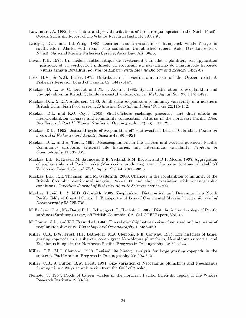
  34

Kawamura, A. 1982. Food habits and prey distributions of three rorqual species in the North Pacific Ocean. Scientific Report of the Whales Research Institute 3$:59-91.

Krieger, K.J., and B.L.Wing. 1985. Location and assessment of humpback whale forage in southeastern Alaska with sonar echo sounding. Unpublished report, Auke Bay Laboratory, NOAA. National Marine Fisheries Service, Auke Bay, AK. 66pp.

Laval, P.H. 1974. Un modele mathematique de l’evitement d’un filet a plankton, son application pratique, et sa verification indirecte en recourant au parasitisme de l’amphipode hyperide Vibilia armata Bovallius. Journal of Experimental Marine Biology and Ecology 14:57-87.

Lorz, H.V., & W.G. Pearcy.1975. Distribution of hyperiid amphipods off the Oregon coast. J. Fisheries Research Board of Canada 32: 1442-1447.

Mackas, D. L., G. C. Louttit and M. J. Austin. 1980. Spatial distribution of zooplankton and phytoplankton in British Columbian coastal waters. Can. J. Fish. Aquat. Sci. 37, 1476-1487.

Mackas, D.L. & E.P. Anderson. 1986. Small-scale zooplankton community variability in a northern British Columbian fjord system. Estuarine, Coastal, and Shelf Science 22:115-142.

Mackas, D.L. and K.O. Coyle. 2005. Shelf-offshore exchange processes, and their effects on mesozooplankton biomass and community composition patterns in the northeast Pacific. Deep Sea Research Part II: Topical Studies in Oceanography 52(5-6): 707-725.

Mackas, D.L., 1992. Seasonal cycle of zooplankton off southwestern British Columbia. Canadian Journal of Fisheries and Aquatic Science 49: 903–921.

Mackas, D.L., and A. Tsuda. 1999. Mesozooplankton in the eastern and western subarctic Pacific: Community structure, seasonal life histories, and interannual variability. Progress in Oceanography 43:335-363.

Mackas, D.L., R. Kieser, M. Saunders, D.R. Yelland, R.M. Brown, and D.F. Moore. 1997. Aggregation of euphausiids and Pacific hake (Merluccius productus) along the outer continental shelf off Vancouver Island. Can. J. Fish. Aquat. Sci. 54: 2080–2096.

Mackas, D.L., R.E. Thomson, and M. Galbraith. 2000. Changes in the zooplankton community of the British Columbia continental margin, 1985-1999, and their covariation with oceanographic conditions. Canadian Journal of Fisheries Aquatic Sciences 58:685-702.

Mackas, David L., & M.D. Galbraith. 2002. Zooplankton Distribution and Dynamics in a North Pacific Eddy of Coastal Origin: I. Transport and Loss of Continental Margin Species. Journal of Oceanography 58:725-738.

McFarlane, G.A., MacDougall, L., Schweigert, J., Hrabok, C. 2005. Distribution and ecology of Pacific sardines (Sardinops sagax) off British Columbia, CA. Cal-COFI Report, Vol. 46.

McGowan, J.A., and V.J. Fraundorf. 1966. The relationship between size of net used and estimates of zooplankton diversity. Limnology and Oceanography 11:456-469.

Miller, C.B., B.W. Frost, H.P. Bathelder, M.J. Clemons, R.E. Conway. 1984. Life histories of large, grazing copepods in a subarctic ocean gyre: Neocalanus plumchrus, Neocalanus cristatus, and Eucalanus bungii in the Northeast Pacific. Progress in Oceangraphy 13: 201-243.

Miller, C.B., M.J. Clemons. 1988. Revised life history analysis for large grazing copepods in the subarctic Pacific ocean. Progress in Oceanography 20: 293-313.

Miller, C.B., J. Fulton, B.W. Frost. 1991. Size variation of Neocalanus plumchrus and Neocalanus flemingeri in a 20-yr sample series from the Gulf of Alaska.

Nemoto, T. 1957. Foods of baleen whales in the northern Pacific. Scientific report of the Whales Research Institute 12:33-89.

  35

Nemoto, T. 1959. Food of baleen whales with reference to whale movements. Scientific Report of the Whales Research Institute 14:149-290.

Nemoto,T. and T. Kasuya. 1965. Foods of baleen whales in the Gulf of Alaska of the North Pacific. Scientific Report of the Whales Research Institute 19:45-51.

O’Connell, M.; Fives, J.M. 1995. The biology of the lesser sand-eel Ammodytes tobianus l. In the Galway Bay area. Biology and Environment. 95b(2): 87-98.

Ohman, M.D., P.E. Smith. 1995. A comparison of zooplankton sampling methods in the Cal-COFI time series. CalCOFI Report Vol. 36.

Ohman, M. 2013. Zooplankton. Crustacean field collection and preservation techniques. DeGrave, Sammy, and Joel Martin, eds. Oxford University Press.

Osgood, K.E., and B.W. Frost. 1994. Comparative life histories of three species of planktonic calanoid copepods in Dabob Bay, Washington. Marine Biology 118: 627-636.

Pankhurst, R.C., D.W. Holder. 1952. Wind tunnel technique. London, Pitman.

Pearcy, W.G. 1983. Quantitative assessment of the vertical distribution of micronektonic fishes with opening/closing midwater trawls. Biological Oceanography 2: 289-310.

Peterson, W.T. 1979. Life history and ecology of Calanus marshallae Forst in the Oregon Upwelling Zone. Dissertation at Oregon State University.

Prakash, A. 1962. Seasonal changes in feeding of coho and spring (Chinook) salmon in southern British Columbian waters. J. Fish. Res. Board. Can. 19:851-866.

Pritchard, A.L., and A.L. Tester. 1944. Food of spring and coho salmon in British Columbia. Bull. Fish. Res. Board Can. 65:23p.

Robards, M.D., M.F. Wilson, R.H. Armstrong, J.F. Piatt. 1999. Sand Lance: a review of biology and predator relations and annotaded bibliography. Res. Pap. PNW-RP-521. Portland, OR: U.S. Department of Agriculture, Forest Service, Pacific Northwest Research Station. 327 p.

Rogers, D.E.; Rabin, D.J.; Rogers, B.J. [and others]. 1979. Seasonal composition and food web relationships of marine organisms in the nearshore zone of Kodiak Island including icthyoplankton, meroplankton (shellfish), zooplankton, and fish. [Seattle, WA]: University of Washington, Fisheries Research Institute, final report FRI-UW-7925: 291 p.

Sameoto, D., N. Cochrane, and A. Herman. 1980. Use of multiple frequency acoustics and other methods in estimating copepod and euphausiid abundances. ICES Theme Session on Measurement of Zooplankton Rates md Biomass Characteristics. C.M. 1990/L:81, Session V. Ref. Theme Session R. 20 p

Sameoto DD, Cochrane N, Herman A (1993) Convergence of acoustic, optical, and net-catch estimates of euphausiid abundance: use of artificial light to reduce net avoidance. Can J Fish Aquat Sci 50:334–346

Schulenberger, E. 1978. Vertical distributions, diurnal migrations, and sampling problems of hyperiid amphipods in the North Pacific central gyre. Deep-Sea Research 25: 605-623.

Scott, J.S. 1973. Food and inferred feeding behavior of northern sand lance (Ammodytes dubius). Journal of theFisheries Research Board of Canada. 30: 451-454.

Shaw, W., and Robinson, C.L.K. 1998. Night versus day abundance estimates of zooplankton at two coastal stations in British Columbia, Canada. Mar. Ecol. Prog. Ser. 175: 143–153.

Smith, P.E., R.I. Clutter. 1965. Hydrodynamics of flow and collection in plankton nets. Ocean science and ocean engineering 1: p.515 (abstract).

  36

Smith, P.E., R.C. Counts, and R.I. Cutter. 1968. Changes in filtering efficiency of plankton nets due to clogging under tow. J. Cons. int. Explor. Mer 32(2):232-248.

Swinney GN, Clarke MR, Maddock L (1986) Influence of an electric light on the capture of oceanic deep-sea fish in Biscay. J Mar Biol Assoc UK 66:483–496

Tanasichuk, R. W. 1998. Interannual variations in the population biology and productivity of Thysanoessa spinifera in Barkley Sound, Canada, with special reference to the 1992 and 1993 warm ocean years. Marine Ecology Progress Series 173: 181-195.

Terazaki, M., C.B. Miller. 1986. Life history and vertical distribution of pelagic chaetognaths at Ocean Station P in the subarctic Pacific. Deep-Sea Research 33: 323-337.

Tomilin, A.G. 1957. Kitoobraznye [Cetacea]. Vol. 9 of Sveri SSSR I Prilezhaschchikh stran [Mammals of the U.S.S.R. and Adjacent Countries]. Izedatel’stvo Akademi Nauk SSSR, Moscow. 756 pp. (Translated by Israel Program for Scientific Translations, 1967, 717 pp., NTIS No. TT 65-50086.)

Tranter, D.J. 1963. Comparison of zooplankton biomass determinations by Indian Ocean standard net, Juday net, and Clarke-Bumpus sampler. Nature, 198:1179--1180.

Tranter, D.J., A.C. Heron 1967. Experiments on filtration in p[lankton nets. Australian Journal of marine Freshwater Research 18:89-111.

Tranter, D.J., Fraser, J.H., eds. 1968. Zooplankton Sampling. Monographs on Oceanographic Methodology 2. Paris. UNESCO Press.

Tranter, D.J., P.E. Smith. 1968. Filtration Performance. In “Monographs on oceanographic methodology 2: Zooplankton Sampling”, UNESCO, Switzerland.

Trevorrow, Mark V., D.L. Mackas, M.C. Benfield. 2005. Comparison of multifrequency acoustic and in situ measurements of zooplankton abundances in Knight Inlet, British Columbia. Journal of the Acoustical Society of America 117 (6):3574-3588.

Trumble, R.J. 1973. Distribution, relative abundance, and general biology of selected underutilized fishery resources of the eastern north Pacific Ocean. Seattle, WA: University of Washington. 178 p. M.S. thesis.

Tsuda, A., H. Saito, H. Kasai. 1999. Life histories of Neocalanus flemingeri and Neocalanus plumhcrus (Calanoida: Copepoda) in the western subarctic Pacific. Marine Biology 135: 533-544.

Tsuda, A., H. Saito, H. Kasai. 2001. Geographical variation of body size of Neocalanus cristatus, N. plumchrus, and N. flemingeri in the Subarctic Pacific and its marginal seas: implications for the origin of large form of N. flemingeri in the Oyashio area. Progress in Oceanography 57:341-352.

Weibe, P.H., S.H. Boyd, B.M. Davis, and J.L. Cox. 1982. Avoidance of towed nets by the euphausiid Nematoscelis megalops. Fishery Bulletin 80(1).

Wiebe, P.C, and M.H. Benfield. 2003. From the Hensen net toward four-dimensional biological oceanography. Progress in Oceanography 56(1):7-136.

Wiebe, P.H., C.J. Ashian, S.M. Gallager, C.S. Davis, G.L. Laweson, N.J. Copley. 2004. Using a high-powered strobe light to increase the catch of Antarctic krill. Marine Biology 144:493-502.

Yamada, Y., T. Ikeda, A. Tsuda. 2004. Comparative life history study on sympatric hyperiid amphipods (Themisto pacifica and T. japonica) in the Oyashio region western North Pacific. Marine Biology 145: 515-527.

  37

Figures & Tables

Figure 1. Schematic for the WP-2 cylindrical-conical net, taken from Tranter & Fraser (1968). The net models we explore in the present study are loosely based on this design.    

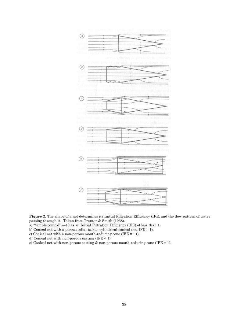
  38

Figure 2. The shape of a net determines its Initial Filtration Efficiency (IFE, and the flow pattern of water passing through it. Taken from Tranter & Smith (1968). a) “Simple conical” net has an Initial Filtration Efficiency (IFE) of less than 1. b) Conical net with a porous collar (a.k.a. cylindrical-conical net; IFE > 1). c) Conical net with a non-porous mouth-reducing cone (IFE =~ 1). d) Conical net with non-porous casting (IFE < 1). e) Conical net with non-porous casting & non-porous mouth reducing cone (IFE = 1).

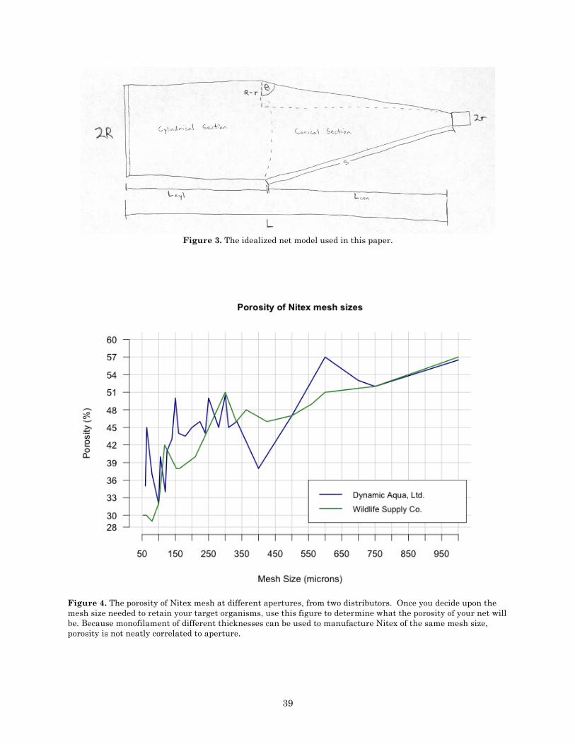
  39

Figure 3. The idealized net model used in this paper.

   

Figure 4. The porosity of Nitex mesh at different apertures, from two distributors. Once you decide upon the mesh size needed to retain your target organisms, use this figure to determine what the porosity of your net will be. Because monofilament of different thicknesses can be used to manufacture Nitex of the same mesh size, porosity is not neatly correlated to aperture.  

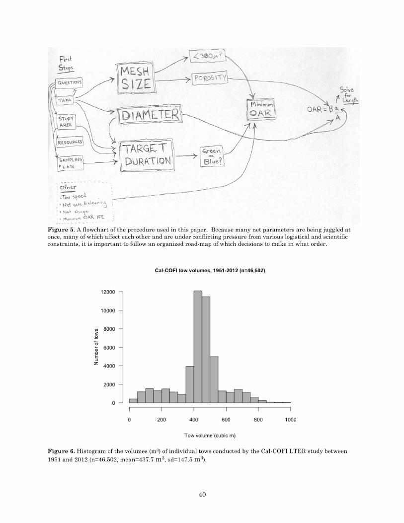
  40

Figure 5. A flowchart of the procedure used in this paper. Because many net parameters are being juggled at once, many of which affect each other and are under conflicting pressure from various logistical and scientific constraints, it is important to follow an organized road-map of which decisions to make in what order.

Figure 6. Histogram of the volumes (m3) of individual tows conducted by the Cal-COFI LTER study between 1951 and 2012 (n=46,502, mean=437.7 m3, sd=147.5 m3).

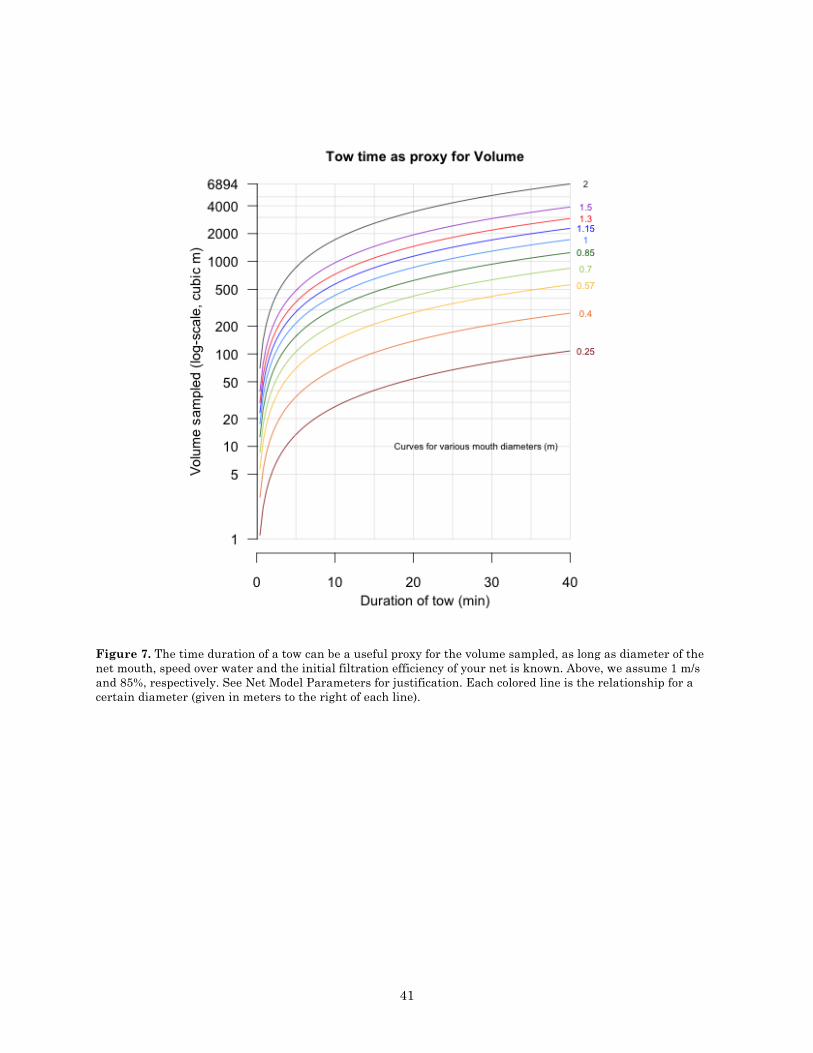
  41

Figure 7. The time duration of a tow can be a useful proxy for the volume sampled, as long as diameter of the net mouth, speed over water and the initial filtration efficiency of your net is known. Above, we assume 1 m/s and 85%, respectively. See Net Model Parameters for justification. Each colored line is the relationship for a certain diameter (given in meters to the right of each line).        

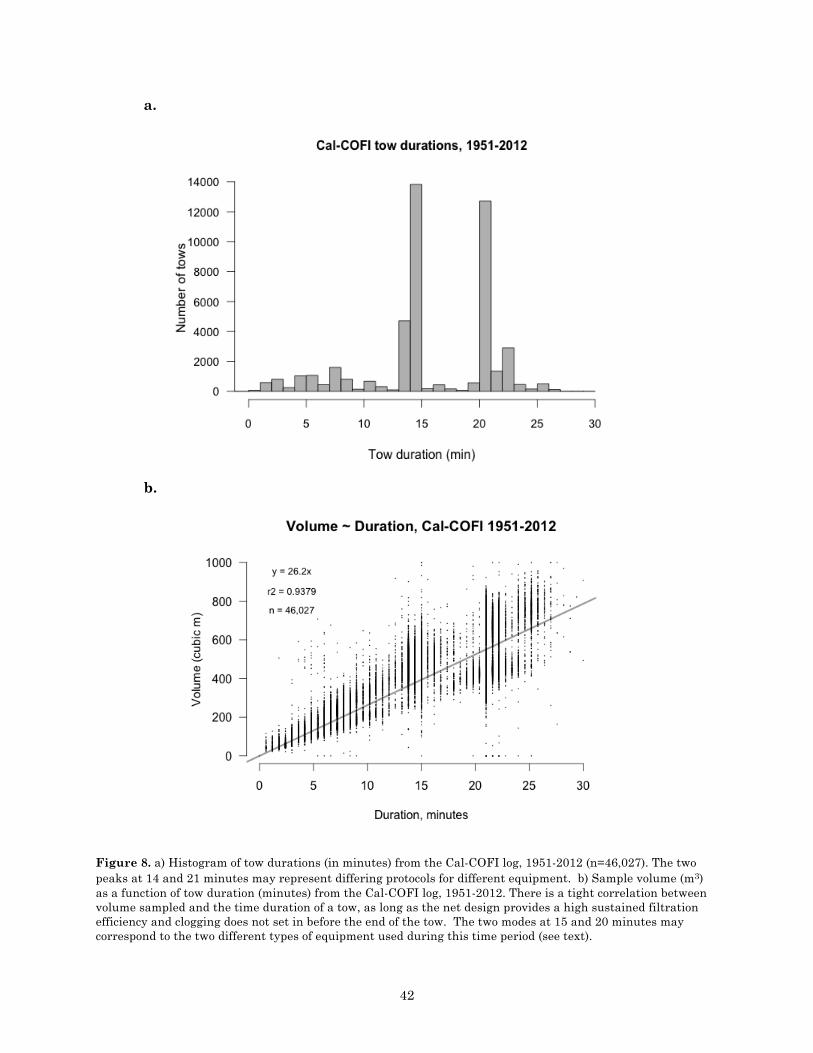
  42

a.

b.

Figure 8. a) Histogram of tow durations (in minutes) from the Cal-COFI log, 1951-2012 (n=46,027). The two peaks at 14 and 21 minutes may represent differing protocols for different equipment. b) Sample volume (m3) as a function of tow duration (minutes) from the Cal-COFI log, 1951-2012. There is a tight correlation between volume sampled and the time duration of a tow, as long as the net design provides a high sustained filtration efficiency and clogging does not set in before the end of the tow. The two modes at 15 and 20 minutes may correspond to the two different types of equipment used during this time period (see text).

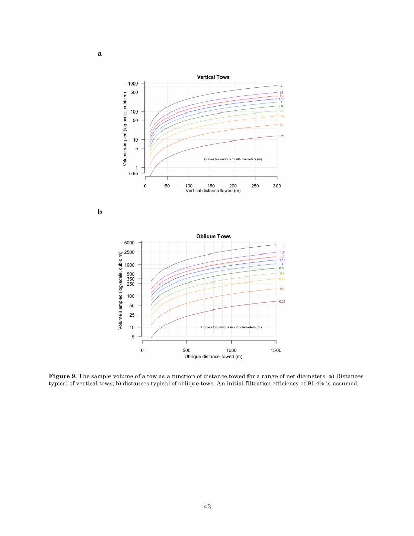
  43

a

b

Figure 9. The sample volume of a tow as a function of distance towed for a range of net diameters. a) Distances typical of vertical tows; b) distances typical of oblique tows. An initial filtration efficiency of 91.4% is assumed.    

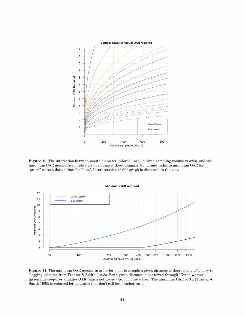
  44

Figure 10. The interaction between mouth diameter (colored lines), desired sampling volume (x axis), and the minimum OAR needed to sample a given volume without clogging. Solid lines indicate minimum OAR for “green” waters, dotted lines for “blue”. Interpretation of this graph is discussed in the text.

Figure 11. The minimum OAR needed in order for a net to sample a given distance without losing efficiency to clogging, adapted from Tranter & Smith (1968). For a given distance, a net towed through “Green waters” (green line) requires a higher OAR than a net towed through blue water. The minimum OAR of 3:1 (Tranter & Smith 1968) is enforced for distances that don’t call for a higher ratio.

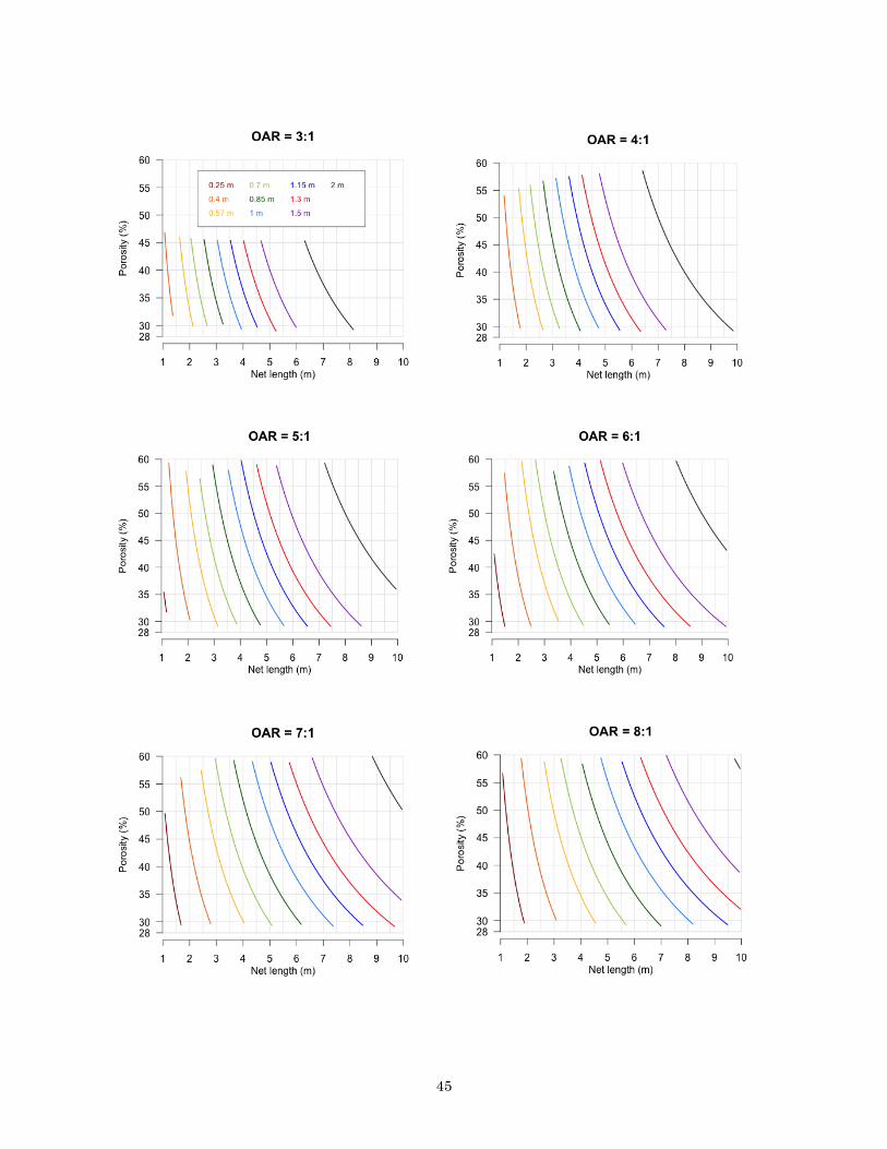
  45

   

   

   

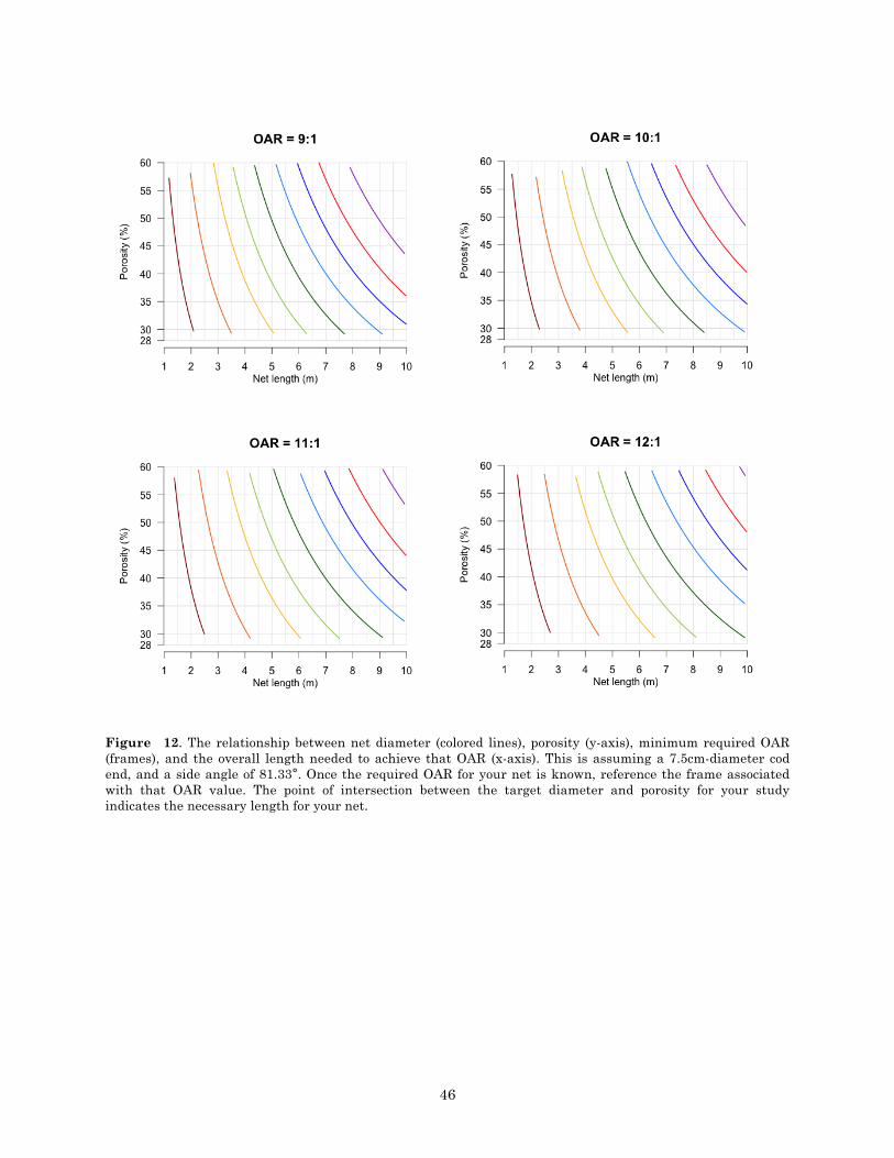
  46

     

     Figure 12. The relationship between net diameter (colored lines), porosity (y-axis), minimum required OAR (frames), and the overall length needed to achieve that OAR (x-axis). This is assuming a 7.5cm-diameter cod end, and a side angle of 81.33°. Once the required OAR for your net is known, reference the frame associated with that OAR value. The point of intersection between the target diameter and porosity for your study indicates the necessary length for your net.      

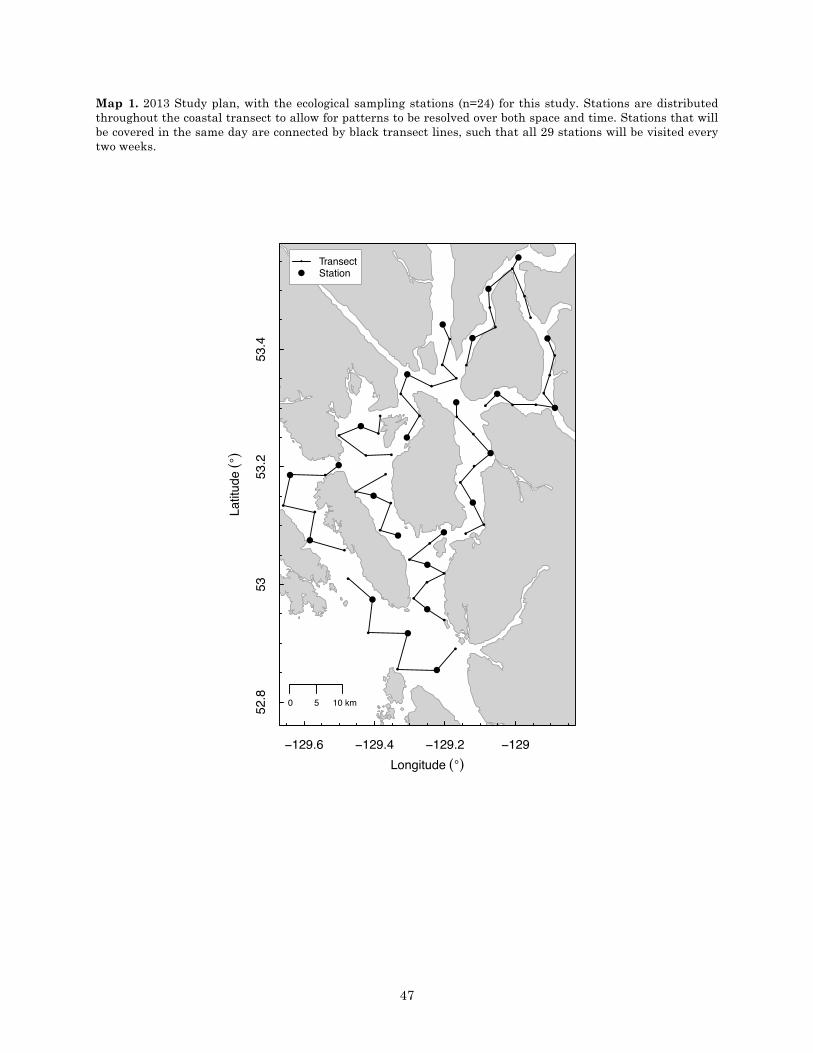
  47

Map 1. 2013 Study plan, with the ecological sampling stations (n=24) for this study. Stations are distributed throughout the coastal transect to allow for patterns to be resolved over both space and time. Stations that will be covered in the same day are connected by black transect lines, such that all 29 stations will be visited every two weeks.

−129.6 −129.4 −129.2 −129

52.8

5353

.253

.4

Longitude (°)

Latit

ude

(°)

●

●●

●●

●

●

●

●

●

●

●

●

●

●

●

●

●

●

●

● ●

●

●

●

● ●●

●

●

●

●

●

●

●

●●

●

●●

●

●

●

●

●

●

●

●

●

●

●

●

●

●

●

●

●

●

●

●

●

●

●

●

●

●

●

●

●

●

●

●

●

●●

●

●●

●●

●

●

●

●

●

●

●

●

●

●

●

●

●

●

●●

●

TransectStation

0 5 10 km

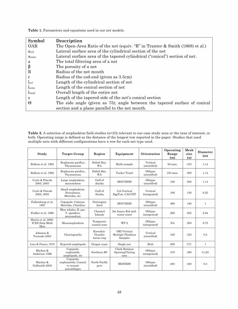
  48

Table 1. Parameters and equations used in our net models. Symbol Description OAR The Open-Area Ratio of the net (equiv. “R” in Tranter & Smith (1968) et al.) acyl Lateral surface area of the cylindrical section of the net acone Lateral surface area of the tapered cylindrical (“conical”) section of net. a The total filtering area of a net β The porosity of a net R Radius of the net mouth r Radius of the cod-end (given as 3.5cm) lcyl Length of the cylindrical section of net lcone Length of the conical section of net ltotal Overall length of the entire net s Length of the tapered side of the net’s conical section Θ The side angle (given as 75); angle between the tapered surface of conical

section and a plane parallel to the net mouth. Table 2. A selection of zooplankton field studies (n=23) relevant to our case study area or the taxa of interest, or both. Operating range is defined as the distance of the longest tow reported in the paper. Studies that used multiple nets with different configurations have a row for each net type used.

Study Target Group Region Equipment Orientation Operating

Range (m)

Mesh size (u)

Diameter (m)

Bollens et al. 1992 Euphausia pacifica,

Thysanoessa Dabob Bay,

WA Multi-sample Vertical

(stratified) 50 max. 333 1.14

Bollens et al. 1992 Euphausia pacifica, Thysanoessa

Dabob Bay, WA

Tucker Trawl Oblique (stratified)

193 max. 500 1.14

Coyle & Pincuk 2005, 2003

Large zooplankton, micronekton

Gulf of Alaska

MOCNESS Oblique (stratified)

100 500 1.14

Coyle & Pincuk 2005, 2003

Small zooplankton: Neocalanus,

Metridia, etc.

Gulf of Alaska

Cal-Vertical EggTow, CALVET

Vertical (integrated) 100 150 0.25

Falkenhaug et al. 1997

Copepods: Calanus, Metridia, Chiridius

Norwegian fjord

MOCNESS Oblique (stratified)

360 180 1

Fiedler et al. 1998 Blue whales, E. pac,

T. spinifera, micronekton

Channel Islands

2m Isaacs-Kid mid-water trawl

Oblique (integrated) 200 505 2.94

Harris et al. 2000. ICES Zoop Meth

Man Mesozooplankton Temperate

coastal zone WP-2 Oblique

(integrated) NA 200 0.75

Johnson & Terazaki 2003 Chaetognaths

Kuroshio-Oyashio

warm-ring

ORI Vertical Multiple Plankton

Sampler

Vertical (stratified) 100 333 0.5

Lorz & Pearcy 1975 Hyperiid amphipods Oregon coast Single-net Both 200 571 1

Mackas & Anderson 1986

Copepods, euphasiids,

amphipods, etc Northern BC

Clark-Bumpus Opening/Closing

nets

Oblique (integrated) 470 390 0.125

Mackas & Galbraith 2002

Copepods, euphausiids; Coastal

vs oceanic assemblages

North Pacific gyre

BIONESS Oblique (stratified)

250 230 0.3

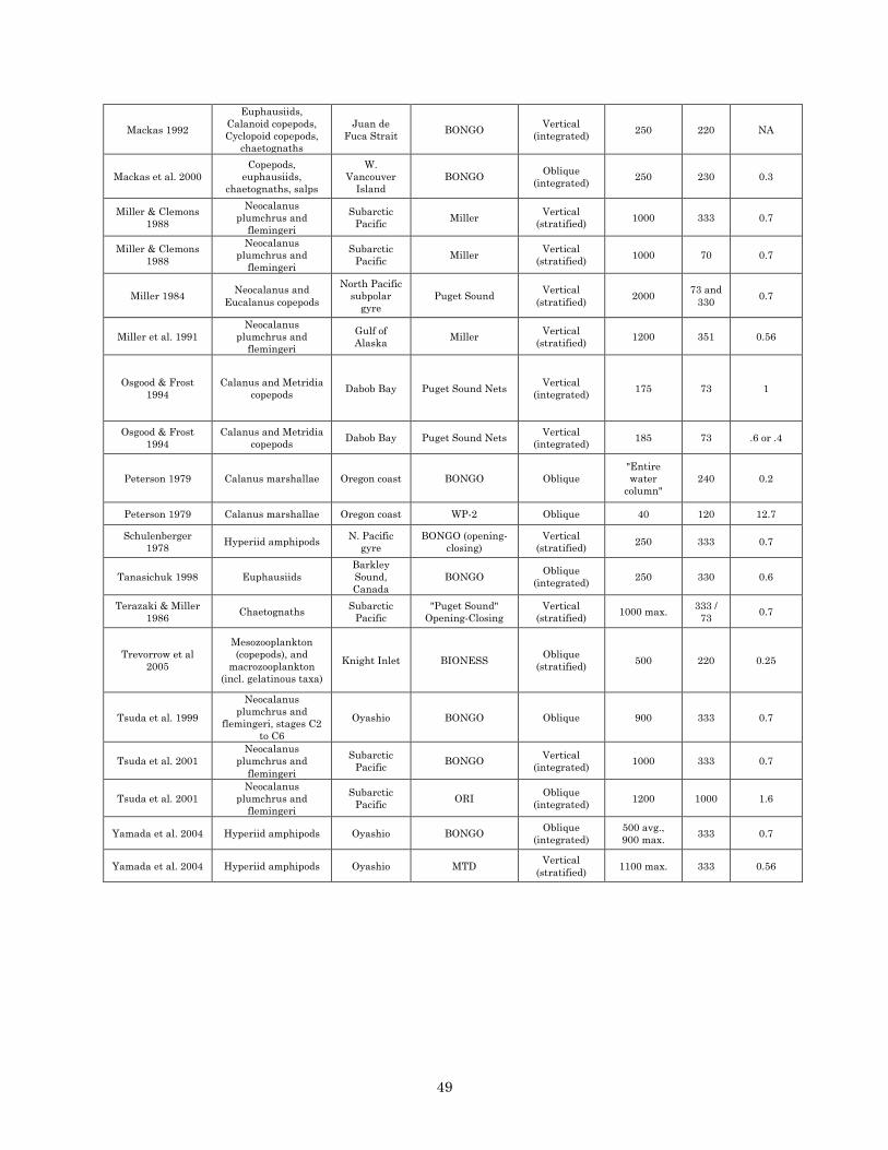
  49

Mackas 1992

Euphausiids, Calanoid copepods, Cyclopoid copepods,

chaetognaths

Juan de Fuca Strait BONGO

Vertical (integrated) 250 220 NA

Mackas et al. 2000 Copepods,

euphausiids, chaetognaths, salps

W. Vancouver

Island BONGO Oblique

(integrated) 250 230 0.3

Miller & Clemons 1988

Neocalanus plumchrus and

flemingeri

Subarctic Pacific Miller

Vertical (stratified) 1000 333 0.7

Miller & Clemons 1988

Neocalanus plumchrus and

flemingeri

Subarctic Pacific Miller

Vertical (stratified) 1000 70 0.7

Miller 1984 Neocalanus and

Eucalanus copepods

North Pacific subpolar

gyre Puget Sound

Vertical (stratified)

2000 73 and

330 0.7

Miller et al. 1991 Neocalanus

plumchrus and flemingeri

Gulf of Alaska

Miller Vertical (stratified)

1200 351 0.56

Osgood & Frost 1994

Calanus and Metridia copepods Dabob Bay Puget Sound Nets

Vertical (integrated) 175 73 1

Osgood & Frost 1994

Calanus and Metridia copepods

Dabob Bay Puget Sound Nets Vertical (integrated)

185 73 .6 or .4

Peterson 1979 Calanus marshallae Oregon coast BONGO Oblique "Entire water

column" 240 0.2

Peterson 1979 Calanus marshallae Oregon coast WP-2 Oblique 40 120 12.7

Schulenberger 1978

Hyperiid amphipods N. Pacific gyre

BONGO (opening-closing)

Vertical (stratified)

250 333 0.7

Tanasichuk 1998 Euphausiids Barkley Sound, Canada

BONGO Oblique

(integrated) 250 330 0.6

Terazaki & Miller 1986

Chaetognaths Subarctic Pacific

"Puget Sound" Opening-Closing

Vertical (stratified)

1000 max. 333 / 73

0.7

Trevorrow et al 2005

Mesozooplankton (copepods), and

macrozooplankton (incl. gelatinous taxa)

Knight Inlet BIONESS Oblique

(stratified) 500 220 0.25

Tsuda et al. 1999

Neocalanus plumchrus and

flemingeri, stages C2 to C6

Oyashio BONGO Oblique 900 333 0.7

Tsuda et al. 2001 Neocalanus

plumchrus and flemingeri

Subarctic Pacific

BONGO Vertical (integrated)

1000 333 0.7

Tsuda et al. 2001 Neocalanus

plumchrus and flemingeri

Subarctic Pacific ORI

Oblique (integrated) 1200 1000 1.6

Yamada et al. 2004 Hyperiid amphipods Oyashio BONGO Oblique (integrated)

500 avg., 900 max.

333 0.7

Yamada et al. 2004 Hyperiid amphipods Oyashio MTD Vertical

(stratified) 1100 max. 333 0.56

 

  50

Table 3. The net inventory of the Scripps Pelagic Invertebrate Collection (SIO PIC) and their estimated open-area ratios (n=123). Columns on net color, condition, and location in the collections have been omitted here. Method of data processing is provided in Appendix 2. Data to left of vertical line and PIC ID# provided by SIO PIC collections manager, Linsey Sala.

Mesh (µ) dmouth (m) dcodend (m) l (m) β OARcyl-cone OARcone PIC ID#

20 0.14 0.09 0.66 0.3 5.42 4.65 115 28 0.3 0.075 1.15 0.3 3.51 2.89 5 40 0.18 0.075 1.2 0.3 7.35 5.67 8 40 0.18 0.075 1.15 0.3 7.02 5.44 9 40 0.18 0.075 1.15 0.3 7.02 5.44 53 0.7 0.075 5 0.3 7.03 4.75 3 53 0.7 0.075 5 0.3 7.03 4.75 6 53 0.3 0.075 1.15 0.3 3.51 2.89 7 53 0.5 0.075 0.95 0.3 0.88 1.34 11 64 0.13 0.08 0.85 0.3 7.57 6.34 96,97 64 0.24 0.08 0.76 0.3 2.95 2.55 98-100

64 0.77 0.11 1.52 0.3 0.95 1.39 101 64 0.2 0.08 0.61 0.3 2.97 2.57 124 64 0.2 0.08 0.28 0.3 0.99 1.2 123 64 0.2 0.06 0.86 0.3 4.22 3.37 134 70 0.3 0.075 1.05 0.3 3.11 2.64 4 75 0.7 0.075 2.6 0.29 2.81 2.4 1 75 0.7 0.075 2.6 0.29 2.81 2.4 2 76 0.2 0.08 0.76 0.29 3.74 3.1 93,94 76 0.22 0.11 0.93 0.29 4.44 3.68 95 76 0.27 0.04 0.38 0.29 0.27 0.98 117

76 0.2 0.06 0.86 0.29 4.08 3.25 135 80 0.13 0.06 0.72 0.29 5.89 4.7 109 86 0.22 0.08 0.85 0.29 3.73 3.07 129 99 0.22 0.08 0.85 0.32 4.12 3.38 128

102 0.5 0.075 2.6 0.32 5.16 3.84 15 102 0.5 0.075 2.7 0.32 5.42 3.99 16 119 0.2 0.13 1.07 0.34 7.02 6.01 88 119 1.14 0.14 2.29 0.34 1.04 1.57 89 120 0.5 0.075 2.3 0.34 4.67 3.61 34 153 0.7 0.075 4.4 0.38 7.6 5.3 21

153 0.7 0.075 4.4 0.38 7.6 5.3 23 153 0.65 0.075 4.9 0.38 9.54 6.4 24 153 0.3 0.075 2.3 0.38 10.28 7.29 33 153 0.41 0.05 0.53 0.38 0.07 1.16 113 153 0.13 0.1 0.76 0.38 8.77 7.86 111 158 0.2 0.08 0.61 0.38 3.76 3.26 84 158 0.22 0.09 0.84 0.38 4.96 4.1 85 158 0.51 0.15 2.06 0.38 4.92 3.99 86 158 1.63 0.18 3.58 0.38 1.39 1.89 87 158 0.23 0.09 0.86 0.38 4.78 3.97 107

158 0.25 0.04 0.38 0.38 0.58 1.39 116 158 0.2 0.13 1.08 0.38 7.92 6.78 110

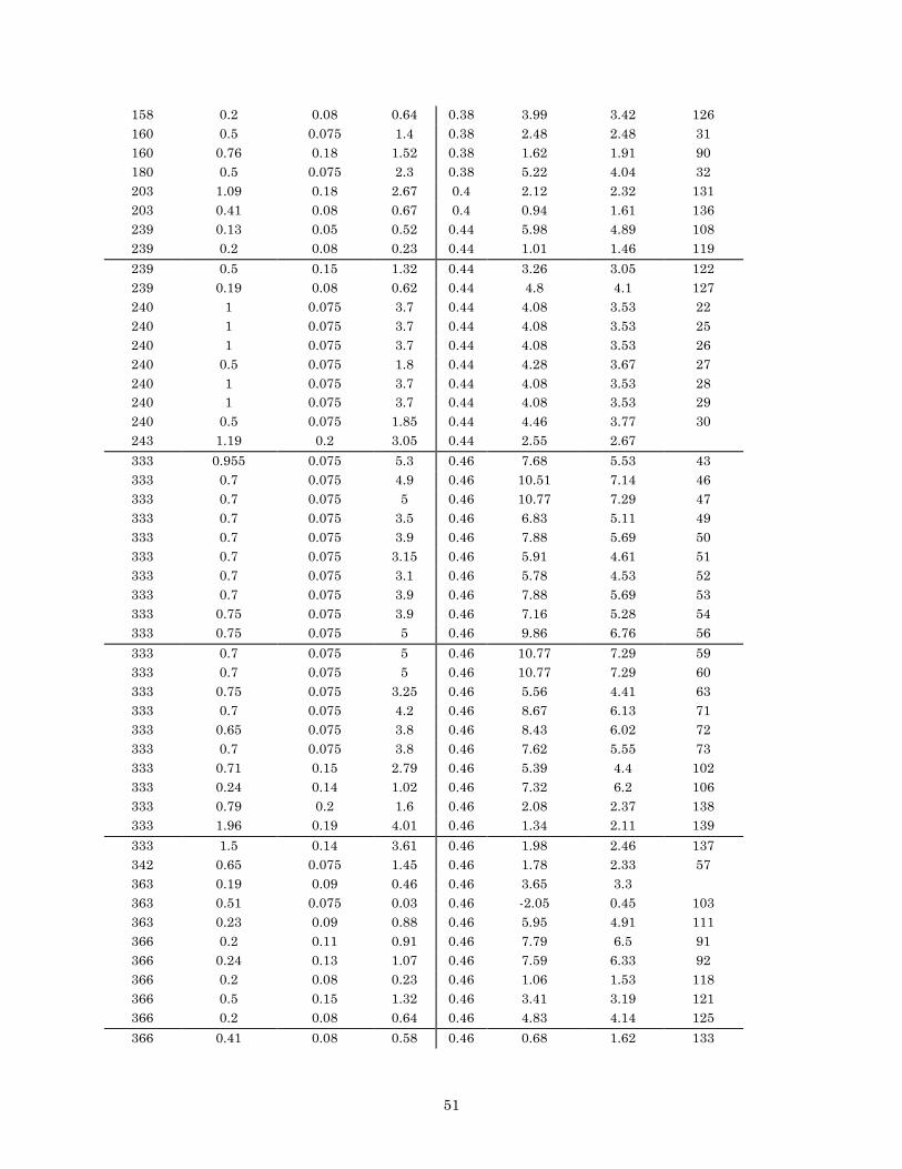
  51

158 0.2 0.08 0.64 0.38 3.99 3.42 126 160 0.5 0.075 1.4 0.38 2.48 2.48 31 160 0.76 0.18 1.52 0.38 1.62 1.91 90 180 0.5 0.075 2.3 0.38 5.22 4.04 32 203 1.09 0.18 2.67 0.4 2.12 2.32 131 203 0.41 0.08 0.67 0.4 0.94 1.61 136 239 0.13 0.05 0.52 0.44 5.98 4.89 108 239 0.2 0.08 0.23 0.44 1.01 1.46 119

239 0.5 0.15 1.32 0.44 3.26 3.05 122 239 0.19 0.08 0.62 0.44 4.8 4.1 127 240 1 0.075 3.7 0.44 4.08 3.53 22 240 1 0.075 3.7 0.44 4.08 3.53 25 240 1 0.075 3.7 0.44 4.08 3.53 26 240 0.5 0.075 1.8 0.44 4.28 3.67 27 240 1 0.075 3.7 0.44 4.08 3.53 28 240 1 0.075 3.7 0.44 4.08 3.53 29 240 0.5 0.075 1.85 0.44 4.46 3.77 30 243 1.19 0.2 3.05 0.44 2.55 2.67

333 0.955 0.075 5.3 0.46 7.68 5.53 43 333 0.7 0.075 4.9 0.46 10.51 7.14 46 333 0.7 0.075 5 0.46 10.77 7.29 47 333 0.7 0.075 3.5 0.46 6.83 5.11 49 333 0.7 0.075 3.9 0.46 7.88 5.69 50 333 0.7 0.075 3.15 0.46 5.91 4.61 51 333 0.7 0.075 3.1 0.46 5.78 4.53 52 333 0.7 0.075 3.9 0.46 7.88 5.69 53 333 0.75 0.075 3.9 0.46 7.16 5.28 54 333 0.75 0.075 5 0.46 9.86 6.76 56

333 0.7 0.075 5 0.46 10.77 7.29 59 333 0.7 0.075 5 0.46 10.77 7.29 60 333 0.75 0.075 3.25 0.46 5.56 4.41 63 333 0.7 0.075 4.2 0.46 8.67 6.13 71 333 0.65 0.075 3.8 0.46 8.43 6.02 72 333 0.7 0.075 3.8 0.46 7.62 5.55 73 333 0.71 0.15 2.79 0.46 5.39 4.4 102 333 0.24 0.14 1.02 0.46 7.32 6.2 106 333 0.79 0.2 1.6 0.46 2.08 2.37 138 333 1.96 0.19 4.01 0.46 1.34 2.11 139

333 1.5 0.14 3.61 0.46 1.98 2.46 137 342 0.65 0.075 1.45 0.46 1.78 2.33 57 363 0.19 0.09 0.46 0.46 3.65 3.3 363 0.51 0.075 0.03 0.46 -2.05 0.45 103 363 0.23 0.09 0.88 0.46 5.95 4.91 111 366 0.2 0.11 0.91 0.46 7.79 6.5 91 366 0.24 0.13 1.07 0.46 7.59 6.33 92 366 0.2 0.08 0.23 0.46 1.06 1.53 118 366 0.5 0.15 1.32 0.46 3.41 3.19 121 366 0.2 0.08 0.64 0.46 4.83 4.14 125

366 0.41 0.08 0.58 0.46 0.68 1.62 133

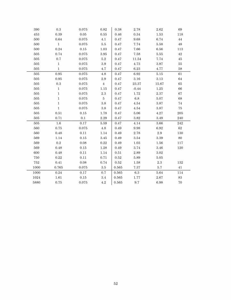
  52

390 0.3 0.075 0.82 0.38 2.78 2.62 69 453 0.39 0.05 0.55 0.46 0.34 1.53 118 500 0.64 0.075 4.1 0.47 9.68 6.74 44 500 1 0.075 5.5 0.47 7.74 5.58 48 500 0.24 0.15 1.03 0.47 7.66 6.56 113 505 0.74 0.075 3.95 0.47 7.58 5.55 42 505 0.7 0.075 5.2 0.47 11.54 7.74 45 505 1 0.075 3.9 0.47 4.73 3.97 55 505 1 0.075 4.7 0.47 6.23 4.77 58

505 0.95 0.075 4.8 0.47 6.92 5.15 61 505 0.95 0.075 2.9 0.47 3.16 3.13 64 505 0.3 0.075 4 0.47 23.37 15.67 65 505 1 0.075 1.15 0.47 -0.44 1.25 66 505 1 0.075 2.3 0.47 1.72 2.37 67 505 1 0.075 5 0.47 6.8 5.07 68 505 1 0.075 3.8 0.47 4.54 3.87 74 505 1 0.075 3.8 0.47 4.54 3.87 75 505 0.51 0.15 1.78 0.47 5.06 4.27 205 505 0.71 0.1 2.29 0.47 3.82 3.49 240

505 1.6 0.17 5.59 0.47 4.14 3.66 242 560 0.75 0.075 4.8 0.49 9.98 6.92 62 560 0.48 0.11 1.14 0.49 2.78 2.9 130 569 1.14 0.15 3.45 0.49 3.54 3.39 80 569 0.2 0.08 0.22 0.49 1.03 1.56 117 569 0.48 0.15 1.28 0.49 3.74 3.46 120 600 0.48 0.11 1.14 0.51 2.89 3.02 750 0.22 0.11 0.71 0.52 5.89 5.05 752 0.41 0.08 0.74 0.52 1.58 2.3 132

1000 0.765 0.075 3.5 0.565 7.37 5.7 41

1000 0.24 0.17 0.7 0.565 6.3 5.64 114 1024 1.61 0.15 3.4 0.565 1.77 2.67 83 5880 0.75 0.075 4.2 0.565 9.7 6.98 70