A Potential Enstrophy and Energy Conserving Scheme … Potential Enstrophy and Energy Conserving Scheme for the Shallow-Water Equations Extended to Generalized Curvilinear Coordinates

A Potential Enstrophy and Energy Conserving Scheme for the Shallow-WaterEquations Extended to Generalized Curvilinear Coordinates

MICHAEL D. TOY AND RAMACHANDRAN D. NAIR

Institute for Mathematics Applied to Geosciences, National Center for Atmospheric Research,a Boulder, Colorado

(Manuscript received 29 June 2016, in final form 3 October 2016)

ABSTRACT

An energy and potential enstrophy conserving finite-difference scheme for the shallow-water equations isderived in generalized curvilinear coordinates. This is an extension of a scheme formulated by Arakawa andLamb for orthogonal coordinate systems. The starting point for the present scheme is the shallow-waterequations cast in generalized curvilinear coordinates, and tensor analysis is used to derive the invariantconservation properties. Preliminary tests on a flat plane with doubly periodic boundary conditions arepresented. The scheme is shown to possess similar order-of-convergence error characteristics using a non-orthogonal coordinate compared to Cartesian coordinates for a nonlinear test of flow over an isolatedmountain.A linear normalmode analysis shows that the discrete form of the Coriolis term provides stationarygeostrophically balanced modes for the nonorthogonal coordinate and no unphysical computational modesare introduced. The scheme uses centered differences and averages, which are formally second-order accu-rate. An empirical test with a steady geostrophically balanced flow shows that the convergence rate of thetruncation errors of the discrete operators is second order. The next step will be to adapt the scheme for use onthe cubed sphere, which will involve modification at the lateral boundaries of the cube faces.

1. Introduction

Arakawa and Lamb (1981, hereafter AL81) de-veloped a finite-difference scheme for the shallow-waterequations that simultaneously conserves energy andpotential enstrophy. As pointed out in subsequent work(e.g., Salmon 2004), this was a significant achievementbecause neither kinetic energy nor potential enstrophyare simple quadratic quantities due to the divergentnature of shallow-water motion. Conserving analogs ofthese two global invariants in numerical models isknown to prevent a spurious cascade of energy towardsmall scales. Direct application ofAL81’s scheme, whichwas derived in rectangular Cartesian coordinates, islimited to orthogonal, quadrilateral grids; however, ithas inspired an active field of research in the develop-ment of schemes that conserve higher-order invariantson generalized grids.AL81’s scheme can be applied directly to global

models that use latitude–longitude grids; however, such

grids suffer from excessive clustering of grid points nearthe poles, which can severely limit the size of the timestep that can be taken. Alternative grid structures with aquasi-uniform distribution of points have been de-veloped to overcome this problem; these include thecubed sphere (Sadourny 1972; Ronchi et al. 1996), theicosahedral geodesic grid (Sadourny et al. 1968;Williamson 1968; Heikes and Randall 1995a,b; Satohet al. 2008; Lee andMacDonald 2009; Bleck et al. 2015),triangular grids (Bonaventura and Ringler 2005;Gassmann 2011), and arbitrarily structured grids basedon Voronoi tessellations (Stuhne and Peltier 2006;Thuburn et al. 2009).The numerical techniques of AL81, developed for

finite-difference equations on orthogonal, quadrilateralgrids, do not easily carry over to these alternative gridstructures, so new techniques have been developed toconserve the various invariant quantities. For example,Ringler and Randall (2002) designed discrete analogs ofthe divergence and curl operators based on their fun-damental, coordinate-invariant definitions that achieveenergy and potential-enstrophy conservation for theshallow-water equations on a geodesic grid. In Thuburnet al. (2009) and Ringler et al. (2010), a conservativescheme, known as TRiSK, was formulated for arbitrarily

a The National Center for Atmospheric Research is sponsoredby the National Science Foundation.

Corresponding author e-mail: Michael D. Toy, [email protected]

MARCH 2017 TOY AND NA IR 751

DOI: 10.1175/MWR-D-16-0250.1

! 2017 American Meteorological Society. For information regarding reuse of this content and general copyright information, consult the AMS CopyrightPolicy (http://www.ametsoc.org/PUBSCopyrightPolicy).

mailto:[email protected]

http://www.ametsoc.org/PUBSCopyrightPolicy



structured locally orthogonal grids. In a follow-up paper,Thuburn and Cotter (2012) extended TRiSK to non-orthogonal grids and formalized the method as a type ofdiscrete exterior calculus (DEC) method (Hirani 2003);however the discretization does not conserve potentialenstrophy. Weller (2014) also developed a scheme fornonorthogonal, arbitrary polygonal grids that nearlyconserves energy and potential enstrophy. In thatpaper, a quasi-orthogonal diamond grid for the cubedsphere was also developed that minimizes errors in-herent with grid nonorthogonality. An issue that ariseswith these schemes is a lack of consistency (i.e., zeroth-order accuracy) of some of the discrete operators. Thisissue has been analyzed on various grids, includingcubed-sphere grids, in Weller (2014) and Thuburnet al. (2014).In a different approach, Salmon (2004, 2007) de-

veloped energy and potential enstrophy conservingschemes for the shallow-water equations on regularsquare grids and unstructured triangular grids usingHamiltonian fluid dynamics. For square grids, Salmonshowed that AL81’s scheme can be derived using thisgeneralized method. Eldred (2015) extended AL81’sscheme to arbitrary nonorthogonal polygonal grids bycombining Hamiltonian and DEC methods, embodyingthe energy and potential-enstrophy conserving proper-ties of AL81.In this paper, we revisit the approach of AL81 for

quadrilateral grids, but instead of starting with thevector-invariant system of equations in rectangularCartesian coordinates, we start with the system ex-pressed in generalized curvilinear coordinates. The re-sult is a finite-difference scheme that exactly conservesmass, energy, and potential enstrophy on generalized(including nonorthogonal) quadrilateral grids with aform almost identical to AL81. In fact, the weightings ofpotential vorticity in the momentum equations, whichare responsible for potential enstrophy conservation,are identical in both schemes. Going to generalizednonorthogonal coordinates is complicated by the ex-pression for kinetic energy involving products of twosets of velocity components: the covariant and contra-variant components, the former being prognostic vari-ables and the latter being diagnostic (e.g., Tort et al.2015). Proper diagnosis of the contravariant compo-nents leads to kinetic energy conservation. Despite thiscomplication, the scheme still possesses the conceptualsimplicity of the AL81 discretization. Also, it is stillbased on centered differences and averages, which areformally second-order accurate. At this point, the schemehas been formulated and tested on a plane surface withdoubly periodic boundary conditions; however, we pro-pose that it could bemodified for application on the cubed

sphere, the challenge being to correctly handle the edgesand corners connecting the cube faces. The scheme couldthen make use of cubic grids based on curvilinear co-ordinate systems for each of the faces, such as thosebased on gnomonic (central) projections (Sadourny1972; Ronchi et al. 1996), which include the equian-gular projections used by Nair et al. (2005a,b), or con-formal (angle preserving) mappings (Ran!cic et al. 1996;McGregor 1996; Adcroft et al. 2004).In section 2 of the paper, we describe the continuous

shallow-water equations in generalized curvilinear co-ordinates and, using tensor analysis, we derive the ten-dency equations for energy, potential vorticity, andpotential enstrophy. In section 3, we derive a finite-difference scheme that conserves both energy and po-tential enstrophy on the staggered Arakawa C grid. Ourstarting point for potential enstrophy conservation isAL81’s scheme itself, and we demonstrate that a par-ticular form of diagnosing the contravariant velocitycomponents leads to kinetic energy conservation. Insection 4, as a first step toward applying the new schemeto the sphere, we test the discrete equations in ashallow-water model on a plane surface with doublyperiodic lateral boundary conditions using a simple,nonorthogonal coordinate transformation. First, we ana-lyze the linear characteristics of the scheme to show thatthere are no unphysical computational modes introducedby the transformation to generalized coordinates, that thenormal modes are all stable, and that stationary geo-strophic modes remain stationary in the discrete system.We then present results of a nonlinear test of flow over anisolated mountain in order to demonstrate the conserva-tion properties of the numerical scheme. The results withthe nonorthogonal coordinate compare well with those ofa run with Cartesian coordinates (i.e., the original schemein AL81). We also compare the resolution-dependent er-ror convergence between the two coordinate systems andshow that the order of convergence is basically maintainedby the extended scheme in AL81, although the error islarger with the nonorthogonal coordinate system. Themodel is then tested under steady-state nonlinear geo-strophic flow in which the exact solution is known, and theoverall discretization error as well as the local truncationerrors of each of the terms in the model equations areshown to possess second-order convergence. Finally, weprovide a summary and discussion in section 5.

2. Continuous equations

To introduce the basic notations for our derivations,we first consider a general 2D coordinate transformationusing classical tensor analysis (e.g., Dutton 1986; Warsi2006; Wesseling 2009).

752 MONTHLY WEATHER REV IEW VOLUME 145

a. Nonorthogonal curvilinear geometry

Consider the coordinate transformation (x, y) /(x1, x2), where x and y are the rectangular Cartesiancoordinates and x15 f1(x, y) and x25 f2(x, y). In gen-eral, the coordinate transformation gives rise to twosets of basis vectors: the ‘‘covariant’’ basis vectors,

ai5

›x

›xi, (1)

and the ‘‘contravariant’’ basis vectors,

ai 5=xi , (2)

where x is the position vector, = is the horizontal gra-dient operator, and i 5 1, 2 is the dimensional index.The covariant metric tensor associated with the trans-formation is defined as Gij 5 ai ! aj, and its inverse is thecontravariant metric tensor Gij, which can be formallydefined as (Warsi 2006)

Gij [›xi

›x

›xj

›x1

›xi

›y

›xj

›y; i, j 2 f1, 2g. (3)

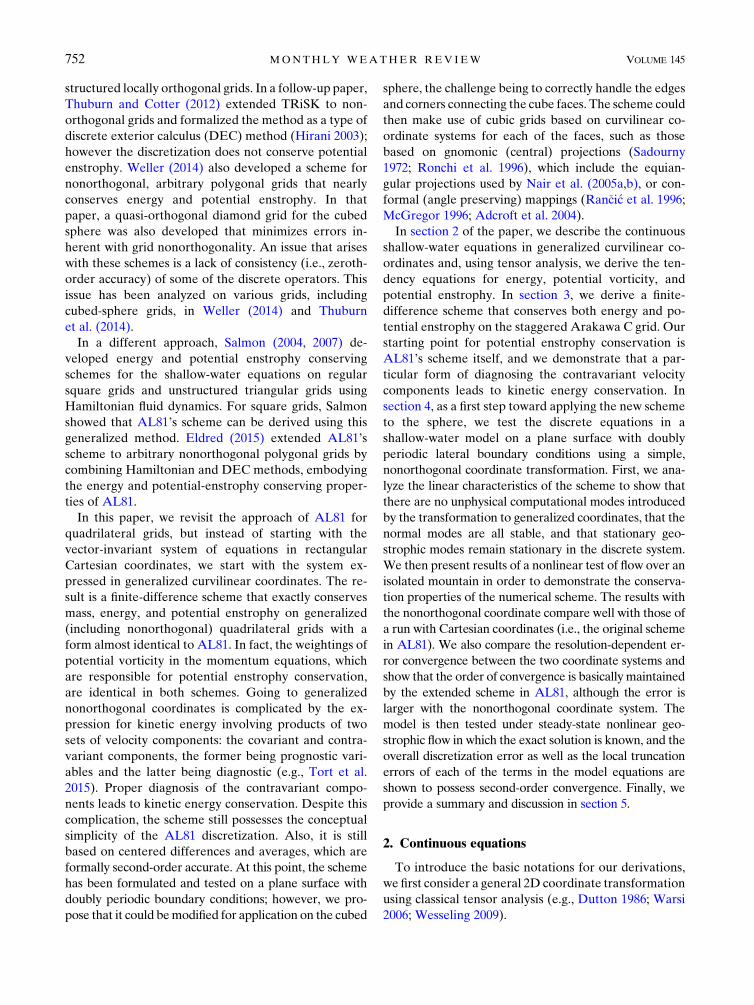
Figure 1 schematically shows a nonorthogonal co-ordinate system (x1, x2) and the covariant and contra-variant basis vectors. Note that in Cartesian coordinates,the basis vectors are the unit vectors i and j. In the caseof nonorthogonal coordinate systems, the two sets ofbasis vectors point in different directions. The covariantbasis vector (ai) corresponding to the ith dimension istangent to coordinate lines of the other dimension, while

the contravariant basis vector (ai) corresponding to theith dimension is normal to coordinate lines of that di-mension (see Fig. 1).In the transformed coordinate system, vectors can be

expressed as linear combinations of either basis vectorset. This gives rise to the covariant velocity components(u1, u2) and the contravariant velocity components(u1, u2), either set being sufficient to specify the velocityin physical space. By convention, the dimensional in-dices of covariant vector components are denoted bysubscripts, while those of contravariant components aredenoted by superscripts. The covariant velocity com-ponents are projections of the velocity onto the co-variant basis vectors, as given by

ui5u ! a

i, (4)

and the contravariant velocity components are pro-jections of the velocity onto the contravariant basisvectors, as given by

ui 5u ! ai , (5)

where u is the velocity. Each set of velocity componentscan be converted to the other using themetric tensorsGij

and Gij through the following relations:

"u1

u2

#5

"G11 G12

G21 G22

#"u1

u2

#and

"u1

u2

#

5

"G

11G

12

G21

G22

#"u1

u2

#

. (6)

The Cartesian x-component and y-component veloci-ties, u and y, respectively, can be diagnosed from thefollowing equations:

u5

!›x1

›x

"u11

!›x2

›x

"u2

y5

!›x1

›y

"u11

!›x2

›y

"u2

9>>>>=

>>>>;

. (7)

Finally, the Jacobian of the coordinate transformation(the metric term), which relates the area elements ineach system, is given by

ffiffiffiffiffiG

p5 jG

ijj1/2 5 ›x

›x1›y

›x22

›x

›x2›y

›x1. (8)

b. Shallow-water equations

The continuity and momentum equations for theshallow-water system (e.g., Sadourny 1972; Nair et al.

FIG. 1. Schematic diagram illustrating a nonorthogonal curvi-linear (x1, x2) grid system and the basis vectors in physical space.The covariant basis vector ai (where i 5 1, 2) is a tangential vector(red), which points along a coordinate line, while the contravariantbasis vector ai (blue) points normally to a coordinate line.


2005a; Bao et al. 2014) can be written in generalizedcurvilinear coordinates as

›

›t(

ffiffiffiffiffiG

ph)1

›

›x1(

ffiffiffiffiffiG

phu1)1

›

›x2(

ffiffiffiffiffiG

phu2)5 0, (9)

›u1

›t1

›

›x1(K1F)5

ffiffiffiffiffiG

phu2q , (10)

and

›u2

›t1

›

›x2(K1F)52

ffiffiffiffiffiG

phu1q , (11)

where h is the fluid depth, K is the kinetic energy,given by

K51

2(u1u1 1 u2u2) , (12)

and F is the geopotential of the free surface, defined as

F[ g(h1 hs) , (13)

where hs is the bottom surface height and g is the grav-itational acceleration. The potential vorticity q is de-fined as

q[f 1 z

h, (14)

where f is the Coriolis parameter, and z is the relativevorticity, given by

z51ffiffiffiffiffiG

p!›u2

›x12›u1

›x2

". (15)

Equations (10) and (11), which are based on thevector invariant form of the momentum equations,have basically the same form as the Cartesian-coordinate equations in AL81. Note that the vorticityin (15) is naturally defined in terms of the covariantvelocity components since they are tangent to co-ordinate surfaces, while the mass-flux terms of thecontinuity equation in (9) are written in terms of thecontravariant components, which are directed nor-mal to coordinate surfaces. Finally, the product

ffiffiffiffiffiG

ph

represents a ‘‘pseudo-density’’ that is related to theamount of mass per unit area in the transformedcoordinate system.We basically follow the same steps as in AL81 to

formulate the conservation of integral invariants such astotal energy, potential vorticity, and potential enstrophyin the generalized coordinate framework. This will serveas a guide for the discrete derivations in the next section.Multiplying (10) by

ffiffiffiffiffiG

phu1 and adding (11) multiplied

byffiffiffiffiffiG

phu2, we get

ffiffiffiffiffiG

ph

!u1›u1

›t1 u2›u2

›t

"1

ffiffiffiffiffiG

phu1›K

›x11

ffiffiffiffiffiG

phu2›K

›x2

1ffiffiffiffiffiG

phu1›F

›x11

ffiffiffiffiffiG

phu2›F

›x25 0. (16)

Using (6) and the fact that themetric tensor is symmetric(i.e., G12 5 G21), the quantity in parentheses on the lhsof (16) can be rearranged as

u1›u1

›t1 u2›u2

›t5u1

›u1

›t1 u2

›u2

›t. (17)

Using (12), we see that this is equivalent to the timetendency of kinetic energy:

u1›u1

›t1u2›u2

›t5

1

2

!u1›u1

›t1 u2›u2

›t

"1

1

2

!u1

›u1

›t1 u2

›u2

›t

"

5›

›t

$1

2(u1u

11u2u

2)

%

5›K

›t.

(18)

Combining (9), (16), and (18) gives the time tendency ofkinetic energy:

›

›t(

ffiffiffiffiffiG

phK)1

›

›x1(

ffiffiffiffiffiG

phu1K)1

›

›x2(

ffiffiffiffiffiG

phu2K)

1ffiffiffiffiffiG

phu1›F

›x11

ffiffiffiffiffiG

phu2›F

›x25 0. (19)

The time tendency of potential energy is obtained bymultiplying (9) by F and rearranging terms to get

›

›t

$ ffiffiffiffiffiG

phg

!1

2h1 h

s

"%1

›

›x1(

ffiffiffiffiffiG

phu1F)1

›

›x2(

ffiffiffiffiffiG

phu2F)

2ffiffiffiffiffiG

phu1›F

›x12

ffiffiffiffiffiG

phu2›F

›x25 0.

(20)

Adding (19) and (20) results in the cancellation of theenergy conversion terms to give the following expres-sion for the time rate of change of total energy:

›

›t

& ffiffiffiffiffiG

ph

$K1 g

!1

2h1 h

s

"%'1

›

›x1[

ffiffiffiffiffiG

phu1(K1F)]

1›

›x2[

ffiffiffiffiffiG

phu2(K1F)]5 0.

(21)

Integrating (21) over the domain results in the followingstatement of the conservation of total energy:

›

›t

& ffiffiffiffiffiG

ph

$K1 g

!1

2h1 h

s

"%'5 0, (22)


where the overbar represents the area integral in x1 andx2 over an infinite domain or over a finite domain withno-flow or periodic boundary conditions.The potential vorticity equation is obtained by com-

bining (10), (11), (14), and (15) to get

›

›t(

ffiffiffiffiffiG

phq)1

›

›x1(

ffiffiffiffiffiG

phu1q)1

›

›x2(

ffiffiffiffiffiG

phu2q)5 0. (23)

This result shows that potential vorticity is globallyconserved. Subtracting (9) times q from (23) and di-viding by

ffiffiffiffiffiG

ph gives

›q

›t1 u1 ›q

›x11u2 ›q

›x25 0. (24)

Multiplying (24) byffiffiffiffiffiG

phq and adding the potential

enstrophy [(1/2)q2] times (9) gives the equation for thetime tendency of potential enstrophy:

›

›t

! ffiffiffiffiffiG

ph1

2q2

"1

›

›x1

! ffiffiffiffiffiG

phu11

2q2

"

1›

›x2

! ffiffiffiffiffiG

phu21

2q2

"5 0, (25)

which, when integrated over the domain, gives an ex-pression for the conservation of potential enstrophy:

›

›t

! ffiffiffiffiffiG

ph1

2q2

"5 0. (26)

In AL81, a finite-difference scheme was derived forthe momentum equations which satisfies the followingrequirements for both divergent and nondivergentflow: that it be consistent with an advection scheme forpotential vorticity such that for a spatially constant q,there is no time change of q, as prescribed by (24);and that it satisfy conservation of total energy and po-tential enstrophy, as given by (22) and (26), respec-tively. In the following section, we show that, due tothe similarity of the governing equations between theCartesian and generalized curvilinear coordinate sys-tems, it is straightforward to carry over the AL81scheme to the generalized coordinate framework, es-pecially for potential enstrophy conservation. How-ever, to satisfy total energy conservation requires anew derivation for nonorthogonal coordinate systemsdue to the form of the kinetic energy given by (12),which involves products of the covariant and contra-variant velocity components. The contravariant ve-locity components must be diagnosed from (6) in sucha way that the relation in (17) is satisfied in the spa-tially discrete system. The difficulty arises due to the

grid staggering and the fact that for nonorthogonalcoordinates, the off-diagonal terms of themetric tensor(i.e., Gij for i 6¼ j) are nonzero.

3. Finite-difference equations

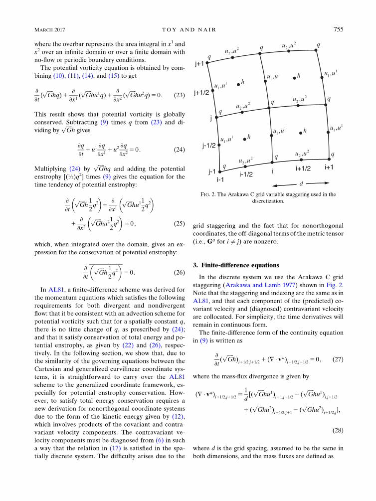
In the discrete system we use the Arakawa C gridstaggering (Arakawa and Lamb 1977) shown in Fig. 2.Note that the staggering and indexing are the same as inAL81, and that each component of the (predicted) co-variant velocity and (diagnosed) contravariant velocityare collocated. For simplicity, the time derivatives willremain in continuous form.The finite-difference form of the continuity equation

in (9) is written as

›

›t(

ffiffiffiffiffiG

ph)

i11/2,j11/2 1 (= ! v*)i11/2,j11/2 5 0, (27)

where the mass-flux divergence is given by

(= ! v*)i11/2,j11/2 [

1

d[(

ffiffiffiffiffiG

phu1)

i11,j11/22 (ffiffiffiffiffiG

phu1)

i,j11/2

1 (ffiffiffiffiffiG

phu2)

i11/2,j112 (ffiffiffiffiffiG

phu2)

i11/2,j],

(28)

where d is the grid spacing, assumed to be the same inboth dimensions, and the mass fluxes are defined as

FIG. 2. The Arakawa C grid variable staggering used in thediscretization.


(ffiffiffiffiffiG

phu1)

i,j11/2 [ [(ffiffiffiffiffiG

ph)(u

1)u1]i,j11/2, (29)

and

(ffiffiffiffiffiG

phu2)

i11/2,j [ [(ffiffiffiffiffiG

ph)(u

2)u2]i11/2,j, (30)

where (ffiffiffiffiffiG

ph)

(u1)

i,j11/2 and (ffiffiffiffiffiG

ph)

(u2)

i11/2,j are theffiffiffiffiffiG

p-weighted

fluid depths interpolated to u1 and u2 points, respectively.Using the flux-form continuity equation in (27) guaranteesmass conservation in the discrete system of equations.Following AL81, we write the discrete form of the

momentum equations in (10) and (11) as

›

›t(u

1)i,j11/22a

i,j11/2(ffiffiffiffiffiG

phu2)

i11/2,j112b


phu2)

i21/2,j112 g


phu2)

i21/2,j2 di,j11/2(

ffiffiffiffiffiG

phu2)

i11/2,j

1 !i11/2,j11/2(

ffiffiffiffiffiG

phu1)

i11,j11/22 !i21/2,j11/2(

ffiffiffiffiffiG

phu1)

i21,j11/2 11

d[(K1F)

i11/2,j11/22 (K1F)i21/2,j11/2]5 0, (31)

and

›

›t(u2)i11/2,j1g

i11,j11/2(ffiffiffiffiffiG

phu1)

i11,j11/2 1 di,j11/2(

ffiffiffiffiffiG

phu1)

i,j11/2 1ai,j21/2(

ffiffiffiffiffiG

phu1)

i,j21/2 1bi11,j21/2(

ffiffiffiffiffiG

phu1)

i11,j21/2

1fi11/2,j11/2(

ffiffiffiffiffiG

phu2)

i11/2,j112fi11/2,j21/2(

ffiffiffiffiffiG

phu2)

i11/2,j21 11

d[(K1F)

i11/2,j11/22 (K1F)i11/2,j21/2]5 0,

(32)

where a, b, g, d, !, and f are linear combinations of the potential vorticity q and K is defined at h points.

a. Conservation of total energy

We now determine the forms of the diagnosed contravariant velocity and kinetic energy required for total energyconservation. Multiplying (31) by (

ffiffiffiffiffiG

phu1)i,j11/2 and (32) by (

ffiffiffiffiffiG

phu2)i11/2,j, using (28)–(30), and summing the re-

sulting equations over the domain results in

!u1pts

›

›t

$(

ffiffiffiffiffiG

ph)(u

1)1

2u1u1

%

i,j11/2

1 !u2pts

›

›t

$(

ffiffiffiffiffiG

ph)(u

2)1

2u2u2

%

i11/2,j

2 !u1pts

$1

2u1u1

›

›t(

ffiffiffiffiffiG

ph)(u

1)%

i,j11/2

2 !u2pts

$1

2u2u2

›

›t(

ffiffiffiffiffiG

ph)(u

2)

%

i11/2,j

2 !hpts

[(K1F)= ! v*]i11/2,j11/2 1

1

2!u1pts

(ffiffiffiffiffiG

ph)

(u1)

i,j11/2

!u1›u1

›t

"

i,j11/2

11

2!u2pts

(ffiffiffiffiffiG

ph)

(u2)

i11/2,j

!u2›u2

›t

"

i11/2,j

21

2!u1pts

(ffiffiffiffiffiG

ph)

(u1)

i,j11/2

!u1

›u1

›t

"

i,j11/2

21

2!u2pts

(ffiffiffiffiffiG

ph)

(u2)

i11/2,j

!u2

›u2

›t

"

i11/2,j

5 0,

(33)

where we used the identity,

!apts

ai,j(bi11/2,j 2b

i21/2,j)52!bpts

bi11/2,j(ai11,j 2 a

i,j), (34)

for two variables a and b defined at staggered i points onthe grid, and a similar identity corresponding to the jindex. Note that, as in the continuous equations, theterms involving q have cancelled out.In the continuous limit, the last four terms on the lhs

of (33) cancel out due to (17). We can achieve cancel-lation of these terms in the discrete system by properlydiagnosing the contravariant velocity components, whichwe write as the discrete form of (6):

(u1)i,j11/2 5 (G11)

i,j11/2(u1)i,j11/21 (G12u

2)(u1)

i,j11/2, (35)

and

(u2)i11/2,j 5 (G21u1)

(u2)

i11/2,j1 (G22)

i11/2,j(u2)i11/2,j, (36)

where (G12u2)(u1)i,j11/2 and (G21u1)

(u2)i11/2,j are interpola-

tions of four neighboring grid points (see Fig. 2). Using(35) and (36), the requirement for cancellation of thelast four terms on the lhs of (33), which is a require-ment for energy conservation in the discrete system,becomes


!u1pts

(ffiffiffiffiffiG

ph)

(u1)

i,j11/2(G12u

2)(u1)

i,j11/2

!›u1

›t

"

i,j11/2

2 !u2pts

(ffiffiffiffiffiG

ph)

(u2)

i11/2,j(u2)i11/2,j

›

›t(G21u

1)(u2)

i11/2,j

2 !u1pts

(ffiffiffiffiffiG

ph)

(u1)

i,j11/2(u1)i,j11/2

›

›t(G12u2)

(u1)

i,j11/21 !

u2pts

(ffiffiffiffiffiG

ph)

(u2)

i11/2,j(G21u1)

(u2)

i11/2,j

!›u

2

›t

"

i11/2,j

5 0. (37)

We assume that

(G12u2)(u1)

i,j11/25

1

(ffiffiffiffiffiG

ph)

(u1)

i,j11/2

A(G12)i,j11/2(G

12)i21/2,j11

ffiffiffiffiffiffiffiffiffiffiffiffiffiffiffiffiffiffiffiffiffiffiffiffiffiffiffiffiffiffiffiffiffiffiffiffiffiffiffiffiffiffiffiffiffiffiffiffiffiffiffiffi(

ffiffiffiffiffiG

ph)

(u1)


ph)

(u2)

i21/2,j11

r(u2)i21/2,j11

"

1B(G12)i,j11/2(G

12)i11/2,j11


ffiffiffiffiffiG

ph)

(u1)


ph)

(u2)

i11/2,j11

r(u

2)i11/2,j11

1C(G12)i,j11/2(G

12)i21/2,j

ffiffiffiffiffiffiffiffiffiffiffiffiffiffiffiffiffiffiffiffiffiffiffiffiffiffiffiffiffiffiffiffiffiffiffiffiffiffiffiffiffiffiffiffiffiffiffiffi(

ffiffiffiffiffiG

ph)

(u1)


ph)

(u2)

i21/2,j

r(u2)i21/2,j

1D(G12)i,j11/2(G

12)i11/2,j


ffiffiffiffiffiG

ph)

(u1)


ph)

(u2)

i11/2,j

r(u

2)i11/2,j

#, (38)

and

(G21u1)(u2)

i11/2,j5

1

(ffiffiffiffiffiG

ph)

(u2)

i11/2,j

E(G12)i11/2,j(G

12)i,j11/2


ffiffiffiffiffiG

ph)

(u2)

i11/2,j(ffiffiffiffiffiG

ph)

(u1)

i,j11/2

r(u1)i,j11/2

"

1F(G12)i11/2,j(G

12)i11,j11/2


ffiffiffiffiffiG

ph)

(u2)


ph)

(u1)

i11,j11/2

r(u

1)i11,j11/2

1G(G12)i11/2,j(G

12)i,j21/2


ffiffiffiffiffiG

ph)

(u2)


ph)

(u1)

i,j21/2

r(u1)i,j21/2

1H(G12)i11/2,j(G

12)i11,j21/2


ffiffiffiffiffiG

ph)

(u2)


ph)

(u1)

i11,j21/2

r(u

1)i11,j21/2

#, (39)

where A thru H are constant coefficients and theoverbars denote averages of neighboring metricterms. There is freedom to use any form of averaging.In the model, whose results are shown in the nextsection, we use the arithmetic mean. The inclusion ofthe fluid depth in the weightings of the covariant ve-locities is a necessary condition for kinetic energyconservation. Note that in orthogonal coordinates, forwhich G12 5 G21 5 0, the rhs of (38) and (39) vanish.Using (38) and (39) in (37), differentiating w.r.t.time, adjusting grid indices, and arranging like termsleads to

A5H; B5G; C5F; D5E . (40)

For consistency, we require

A1B1C1D5 1; E1F1G1H5 1. (41)

We then choose

A5B5C5D5E5F5G5H5 1/4. (42)

With the contravariant velocity components given by (35),(36), (38), (39), and (42), we can finally rewrite (33), thetime tendency of total kinetic energy, as

!u1pts

›

›t

$(

ffiffiffiffiffiG

ph)(u

1)1

2u1u

1

%

i,j11/2

1 !u2pts

›

›t

$(

ffiffiffiffiffiG

ph)(u

2)1

2u2u

2

%

i11/2,j

2 !u1pts

$1

2u1u

1

›

›t(

ffiffiffiffiffiG

ph)(u

1)%

i,j11/2

2 !u2pts

$1

2u2u

2

›

›t(

ffiffiffiffiffiG

ph)(u

2)%

i11/2,j

2 !h pts

[(K1F)= ! v*]i11/2,j11/2 5 0. (43)


When we choose

(ffiffiffiffiffiG

ph)

(u1)

i,j11/2 5 (ffiffiffiffiffiG

ph)

i

i,j11/2, (44)

and

(ffiffiffiffiffiG

ph)

(u2)

i11/2,j 5 (ffiffiffiffiffiG

ph)

j

i11/2,j, (45)

in the definition of the mass fluxes given by (29) and(30), where the overbars ( )

iand ( )

jdenote the

arithmetic average of two neighboring points in the x1

and x2 directions, respectively, we can use the fol-lowing identity for any variables a and b on a stag-gered grid,

!apts

ai,j(b

i)i,j 5 !

bptsbi11/2,j(a

i)i11/2,j, (46)

and the corresponding identity for the j index, to rewrite(43) as

!hpts

›

›t

$(

ffiffiffiffiffiG

ph)

1

2(u1u

1

i1 u2u

2

j)

%

i11/2,j11/2

2 !hpts

(F= ! v*)i11/2,j11/2

2 !hpts

$1

2(u1u

1i1 u2u

2j)

%

i11/2,j11/2

›

›t(

ffiffiffiffiffiG

ph)

i11/2,j11/2 2 !hpts

Ki11/2,j11/2(= ! v*)

i11/2,j11/2 5 0. (47)

As a result, the discrete form of the kinetic energy isdetermined by kinetic energy conservation as

Ki11/2,j11/2 5

1

2(u

1u1

i1 u

2u2

j)i11/2,j11/2. (48)

Using (48) and (27) in (47), the statement of kineticenergy conservation becomes

!hpts

›

›t(

ffiffiffiffiffiG

phK)

i11/2,j11/2 2 !hpts

(F= ! v*)i11/2,j11/2 5 0. (49)

The time tendency of total potential energy is ob-tained by multiplying (27) by Fi11/2,j11/2 and summingover the domain, which results in

!hpts

›

›t

$ ffiffiffiffiffiG

phg

!1

2h1 h

s

"%

i11/2,j11/2

1 !hpts

(F= ! v*)i11/2,j11/2 5 0. (50)

Adding (49) and (50) shows that total energy is con-served by the discretization:

!hpts

›

›t

& ffiffiffiffiffiG

ph

$K1 g

!1

2h1 h

s

"%'

i11/2,j11/2

5 0. (51)

b. Conservation of potential enstrophy

The derivation of the discrete form of potentialenstrophy conservation follows directly from AL81when we define the discrete form of q, defined at (i, j)points, as

qij[( f 1 z)

i,j

h(q)i,j

, (52)

where

zi,j[

1

(ffiffiffiffiffiG

p)i,jd

[(u1)i,j21/22(u

1)i,j11/21(u

2)i11/2,j2(u

2)i21/2,j],

(53)

h(q)i,j 5(

ffiffiffiffiffiG

ph)

(q)

i,j

(ffiffiffiffiffiG

p)i,j

, (54)

and

(ffiffiffiffiffiG

ph)

(q)

i,j 51

4[(

ffiffiffiffiffiG

ph)

i11/2,j11/2 1 (ffiffiffiffiffiG

ph)

i21/2,j11/2

1 (ffiffiffiffiffiG

ph)

i21/2,j21/2 1 (ffiffiffiffiffiG

ph)

i11/2,j21/2]. (55)

Combining (31), (32), and (52)–(54) gives the finite-difference vorticity equation:


›

›t[(

ffiffiffiffiffiG

ph)(q)q]

i,j 51

d[2(

ffiffiffiffiffiG

phu2)

i11/2,j11(ai,j11/2 1fi11/2,j11/2)2 (

ffiffiffiffiffiG

phu2)

i21/2,j11(bi,j11/2 2fi21/2,j11/2)

1 (ffiffiffiffiffiG

phu2)

i11/2,j(ai,j21/2 2 di,j11/2)1 (

ffiffiffiffiffiG

phu2)

i21/2,j(bi,j21/2 2 gi,j11/2)

1 (ffiffiffiffiffiG

phu2)

i11/2,j21(di,j21/2 1fi11/2,j21/2)1 (

ffiffiffiffiffiG

phu2)

i21/2,j21(gi,j21/2 2fi21/2,j21/2)

2 (ffiffiffiffiffiG

phu1)

i11,j11/2(gi11,j11/2 2 !i11/2,j11/2)2 (

ffiffiffiffiffiG

phu1)

i,j11/2(di,j11/2 2 gi,j11/2)

1 (ffiffiffiffiffiG

phu1)

i21,j11/2(di21,j11/2 2 !i21/2,j11/2)2 (

ffiffiffiffiffiG

phu1)

i11,j21/2(bi11,j21/2 1 !i11/2,j21/2)

2 (ffiffiffiffiffiG

phu1)

i,j21/2(ai,j21/2 2bi,j21/2)1 (

ffiffiffiffiffiG

phu1)

i21,j21/2(ai21,j21/2 1 !i21/2,j21/2)]. (56)

Potential vorticity is shown to be globally conserved, as in AL81, by summing (56) over all vorticity points, re-arranging indices, and canceling like terms to obtain

!qpts

›

›t[(

ffiffiffiffiffiG

ph)(q)q]

i,j 5 0. (57)

Combining (27), (28), and (55) gives the continuity equation at q points:

›

›t(

ffiffiffiffiffiG

ph)

(q)

i,j 521

4df[(

ffiffiffiffiffiG

phu2)

i11/2,j112 (

ffiffiffiffiffiG

phu2)


phu1)


phu1)

i,j11/2]

1 [(ffiffiffiffiffiG

phu2)


phu2)


phu1)

i,j11/22 (ffiffiffiffiffiG

phu1)

i21,j11/2]


phu2)


phu2)

i21/2,j211 (

ffiffiffiffiffiG

phu1)

i,j21/22 (ffiffiffiffiffiG

phu1)

i21,j21/2]


phu2)


phu2)

i11/2,j21 1 (ffiffiffiffiffiG

phu1)


phu1)

i,j21/2]g. (58)

Noting that

(ffiffiffiffiffiG

ph)

(q)

i,j

›qi,j

›t5

›

›t[(

ffiffiffiffiffiG

ph)(q)q]

i,j2 qi,j

›

›t(

ffiffiffiffiffiG

ph)

(q)

i,j , (59)

we can subtract (58) multiplied by qi,j from (56) to get

(ffiffiffiffiffiG

ph)

(q)

i,j

›qi,j

›t5

1

d

$2(

ffiffiffiffiffiG

phu2)

i11/2,j11

!ai,j11/2 1f

i11/2,j11/2 2qi,j

4

"2 (

ffiffiffiffiffiG

phu2)

i21/2,j11

!bi,j11/2 2f

i21/2,j11/2 2qi,j

4

"

1 (ffiffiffiffiffiG

phu2)

i11/2,j(ai,j21/2 2 di,j11/2)1 (

ffiffiffiffiffiG

phu2)

i21/2,j(bi,j21/2 2 gi,j11/2)

1 (ffiffiffiffiffiG

phu2)

i11/2,j21

!di,j21/2 1f

i11/2,j21/2 2qi,j

4

"1 (

ffiffiffiffiffiG

phu2)

i21/2,j21

!gi,j21/2 2f

i21/2,j21/2 2qi,j

4

"

2 (ffiffiffiffiffiG

phu1)

i11,j11/2

!gi11,j11/2 2 !

i11/2,j11/2 2qi,j

4

"2 (

ffiffiffiffiffiG

phu1)

i,j11/2(di,j11/2 2 gi,j11/2)

1 (ffiffiffiffiffiG

phu1)

i21,j11/2

!di21,j11/2 2 !

i21/2,j11/2 2qi,j

4

"2 (

ffiffiffiffiffiG

phu1)

i11,j21/2

!bi11,j21/2 1 !

i11/2,j21/2 2qi,j

4

"

2 (ffiffiffiffiffiG

phu1)

i,j21/2(ai,j21/2 2bi,j21/2)1(

ffiffiffiffiffiG

phu1)

i21,j21/2

!ai21,j21/2 1 !

i21/2,j21/2 2qi,j

4

"%.

(60)


Multiplying (60) by qi,j and adding (1/2)q2i,j times (58) gives the potential enstrophy equation:

›

›t

$(

ffiffiffiffiffiG

ph)(q)

1

2q2

%

i,j

5qi,j

d

$2(

ffiffiffiffiffiG

phu2)

i11/2,j11

!ai,j11/2 1f

i11/2,j11/2 2qi,j

8

"

2 (ffiffiffiffiffiG

phu2)

i21/2,j11

!bi,j11/2 2f

i21/2,j11/2 2qi,j

8

"1 (

ffiffiffiffiffiG

phu2)

i11/2,j(ai,j21/2 2 di,j11/2)

1 (ffiffiffiffiffiG

phu2)

i21/2,j(bi,j21/2 2 gi,j11/2)1 (

ffiffiffiffiffiG

phu2)

i11/2,j21

!di,j21/2 1f

i11/2,j21/2 2qi,j

8

"

1 (ffiffiffiffiffiG

phu2)

i21/2,j21

!gi,j21/2 2f

i21/2,j21/2 2qi,j

8

"2 (

ffiffiffiffiffiG

phu1)

i11,j11/2

!gi11,j11/2 2 !

i11/2,j11/2 2qi,j

8

"

2 (ffiffiffiffiffiG

phu1)

i,j11/2(di,j11/2 2 gi,j11/2)1 (

ffiffiffiffiffiG

phu1)

i21,j11/2

!di21,j11/2 2 !

i21/2,j11/2 2qi,j

8

"

2 (ffiffiffiffiffiG

phu1)

i11,j21/2

!bi11,j21/2 1 !

i11/2,j21/2 2qi,j

8

"2 (

ffiffiffiffiffiG

phu1)

i,j21/2(ai,j21/2 2bi,j21/2)

1 (ffiffiffiffiffiG

phu1)

i21,j21/2

!ai21,j21/2 1 !

i21/2,j21/2 2qi,j

8

"%.

(61)

When the linear combinations of potential vorticity arespecified as in AL81,

!i11/2,j11/2 5

1/24(qi11,j11 1 q

i,j11 2 qi,j 2 q

i11,j)

fi11/2,j11/2 5

1/24(2qi11,j11 1q

i,j11 1 qi,j 2 q

i11,j)

ai,j11/2 5

1/24(2qi11,j11

1 qi,j11

1 2qi,j 1 q

i11,j)

bi,j11/2 5

1/24(qi,j11

1 2qi21,j11

1 qi21,j 1 2q

i,j)

gi,j11/2 5

1/24(2qi,j11 1 q

i21,j11 1 2qi21,j 1 q

i,j)

di,j11/2 5

1/24(qi11,j11 1 2q

i,j11 1 qi,j 1 2q

i11,j)

9>>>>>>>>>>>>>>>>>>=

>>>>>>>>>>>>>>>>>>;

, (62)

and they are used in (61) and summed over the domain,the result is the following statement of the conservationof potential enstrophy:

!qpts

›

›t

$(

ffiffiffiffiffiG

ph)(q)

1

2q2

%

i,j

5 0. (63)

In summary, (27)–(32), (35), (36), (38), (39), (42),(44), (45), (48), (52)–(55), and (62) describe the en-ergy and potential enstrophy conserving scheme for theshallow-water equations in generalized curvilinear co-ordinates. In Cartesian coordinates, the scheme reducesexactly to AL81. We should also note that the schemesatisfies the requirement that there be no time changeof potential vorticity for a spatially constant q, whichfollows from the continuous potential vorticity equationin (24), since the rhs of (60) vanishes for a constant qapplied in (62).

4. Results on a plane surface

The shallow-water equations described in the pre-vious sections are based on the vector invariant form ofthe momentum equations, which can be used on curvedsurfaces, such as the sphere. In this section, for sim-plicity, we test the finite-difference scheme on a planesurface with doubly periodic lateral boundary condi-tions and prescribe a simple nonorthogonal coordinatetransformation that is also doubly periodic. We examinethe linear aspects of the discretized system and evaluatethe conservation properties in a nonlinear simulation.Results are compared between the nonorthogonal cur-vilinear coordinate and Cartesian coordinates, in whichthe scheme is equivalent to AL81.

a. Description of the domain and coordinatetransformation

The 2D model domain is a flat plane that extends adistance of 2pa in each Cartesian (x, y) dimension,where a5 6.373 106m is Earth’s radius, and the lateralboundaries are doubly periodic. The coordinate trans-formation used in the experiments is given by

x1 5 x11

2a sin

y

a

x2 5 y1 a sinx

a

9>>=

>>;, (64)

which is plotted in Fig. 3. This is a simple, nonorthogonaltransformation for testing the finite-difference scheme,and is periodic at the lateral boundaries to facilitateevaluation of globally conserved quantities. Note thatthe transformed coordinate has the units of meters.


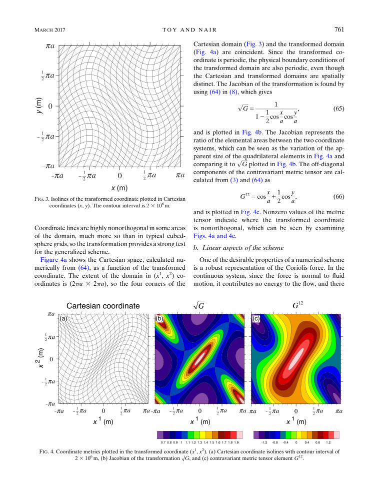
Coordinate lines are highly nonorthogonal in some areasof the domain, much more so than in typical cubed-sphere grids, so the transformation provides a strong testfor the generalized scheme.Figure 4a shows the Cartesian space, calculated nu-

merically from (64), as a function of the transformedcoordinate. The extent of the domain in (x1, x2) co-ordinates is (2pa 3 2pa), so the four corners of the

Cartesian domain (Fig. 3) and the transformed domain(Fig. 4a) are coincident. Since the transformed co-ordinate is periodic, the physical boundary conditions ofthe transformed domain are also periodic, even thoughthe Cartesian and transformed domains are spatiallydistinct. The Jacobian of the transformation is found byusing (64) in (8), which gives

ffiffiffiffiffiG

p5

1

121

2cos

x

acos

y

a

, (65)

and is plotted in Fig. 4b. The Jacobian represents theratio of the elemental areas between the two coordinatesystems, which can be seen as the variation of the ap-parent size of the quadrilateral elements in Fig. 4a andcomparing it to

ffiffiffiffiffiG

pplotted in Fig. 4b. The off-diagonal

components of the contravariant metric tensor are cal-culated from (3) and (64) as

G12 5 cosx

a1

1

2cos

y

a, (66)

and is plotted in Fig. 4c. Nonzero values of the metrictensor indicate where the transformed coordinateis nonorthogonal, which can be seen by examiningFigs. 4a and 4c.

b. Linear aspects of the scheme

One of the desirable properties of a numerical schemeis a robust representation of the Coriolis force. In thecontinuous system, since the force is normal to fluidmotion, it contributes no energy to the flow, and there

FIG. 4. Coordinate metrics plotted in the transformed coordinate (x1, x2). (a) Cartesian coordinate isolines with contour interval of2 3 106m, (b) Jacobian of the transformation OG, and (c) contravariant metric tensor element G12.

FIG. 3. Isolines of the transformed coordinate plotted in Cartesiancoordinates (x, y). The contour interval is 2 3 106m.


exist stationary geostrophically balanced modes. How-ever, in discrete systems there is the possibility of non-stationary geostrophic modes (Thuburn 2008; Thuburnet al. 2009; Eldred 2015). The AL81 scheme avoids suchartificial nonstationary modes, which is one of its desir-able features. Here we determine whether the geo-strophically balanced modes are stationary in the schemeextended to generalized, nonorthogonal curvilinear co-ordinates. Another concern with the generalized schemethat we will investigate is the possible introduction ofcomputational modes due to the four-point averaging ofthe covariant velocities [Eqs. (38) and (39)] used to di-agnose the contravariant velocities.Whenwe assume a constant Coriolis parameter f, then

the continuous dispersion relation for the f-planeshallow-water equations linearized about a resting basicstate and no bottom topography can be derived analyt-ically (e.g., Randall 1994) as

v[v2 2 gh0(k2 1m2)2 f 2]5 0, (67)

where v is the frequency, h0 is the basic-state fluid depth,and k and m are the wavenumbers in the x and y di-rections, respectively. The v 5 0 solutions are the sta-tionary geostrophic modes, while the nonzero-frequencymodes correspond to mixed inertio-gravity waves.The discrete linear system of equations is shown in

appendix A. Inspection of the linearized Coriolis termson the rhs of (A6) and (A7) reveals that the discreteform of the terms are consistent, that is, as the gridspacing vanishes, the metric terms converge to the samevalue such that (A8) and (A9) converge to the contin-uous form in (6), causing the Coriolis terms in (A6) and(A7) to converge to the continuous forms

ffiffiffiffiffiG

pfu2 and

2ffiffiffiffiffiG

pfu1, respectively. For the normal-mode analysis,

we assume that the time-dependent part of the solutionhas the form eivt, so we can write

›

›t(h)

i11/2,j11/2 5 iv(h)i11/2,j11/2

›

›t(u

1)i,j11/25 iv(u

1)i,j11/2

›

›t(u2)i11/2,j5 iv(u2)i11/2,j

9>>>>>>>=

>>>>>>>;

. (68)

The system in (A5)–(A9) for i 5 1, 2, 3, . . . , N andj5 1, 2, 3, . . . ,N, whereN is the number of grid points ineach dimension, then forms an eigenvalue problem inwhich the eigenvalues v are the normal mode frequen-cies. The existence of nonzero imaginary components ofv imply exponential growth of unstable modes.We computed the eigenmodes numerically for the

domain described in section 4a with 16 3 16 evenly

spaced grid points, giving a spacing of d 5 (1/8)pa ineach coordinate direction. The Coriolis parameter wasset to f 5 0.0001 s21, a value of g 5 9.81m s21 was usedfor gravity, and the basic-state fluid depth was h0 55960m. We computed the normal modes for Cartesiancoordinates by setting

ffiffiffiffiffiG

p5G11 5G22 5 1 andG12 5 0;

for the nonorthogonal coordinate transformation, weused (64). For both coordinate systems, all the imaginarycomponents of frequency were found to be zero withinround-off error, and the geostrophic modes were sta-tionary (i.e., v 5 0) also to within round-off error. Inappendix B, we show analytically that the nondivergentgeostrophic modes are indeed stationary. Therefore, theAL81 scheme extended to nonorthogonal, curvilinearcoordinates does not introduce unstable computationalmodes or nonstationary geostrophic modes.The dispersion relations for the discrete system in each

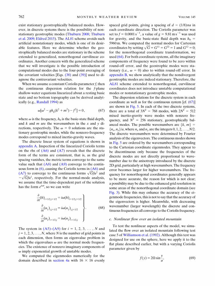
coordinate as well as for the continuous system [cf. (67)]are shown in Fig. 5. In each of the two discrete systems,there are a total of 3N2 5 768 modes, with 2N2 5 512mixed inertio-gravity wave modes with nonzero fre-quency, and N2 5 256 stationary, geostrophically bal-anced modes. The possible wavenumbers are fk, mg 5fnx, nyg/a, where nx and ny are the integers 0, 1, 2, . . . ,N/2.The discrete wavenumbers were determined by Fourieranalysis of the eigenvectors. The continuousmodes shownin Fig. 5 are ordered by the wavenumbers correspondingto the Cartesian coordinate eigenmodes. They appear tobe discontinuous only because the frequencies of thediscrete modes are not directly proportional to wave-number due to the anisotropy introduced by the discrete2D grid, particularly at high wavenumbers. The frequencyerror becomes larger for higher wavenumbers. The fre-quency for nonorthogonal coordinates generally appearsto be more accurate, the reason for which is not clear;a possibilitymay be due to the enhanced grid resolution insome areas of the nonorthogonal coordinate domain (seeFig. 3). While this may enhance the accuracy of the ei-genmode frequencies, this is not to say that the accuracy ofthe eigenvectors is higher. Meanwhile, with decreasingwavenumber (larger wavelength) the discrete and con-tinuous frequencies all converge to theCoriolis frequency.

c. Nonlinear flow over an isolated mountain

To test the nonlinear aspects of the model, we simu-lated the flow over an isolated mountain following testcase 5 ofWilliamson et al. (1992). Although this test wasdesigned for use on the sphere, here we apply it to theflat plane described earlier, but with a varying Coriolisparameter given by

f (y)5 2V siny

a, (69)


whereV5 7.2923 1025 s21 is the rotation rate of Earth.Note that the Coriolis parameter is periodic in the ydomain, which spans f2pa# y# pag. Physically, this istwice the great-circle distance between Earth’s poles,therefore, the domain is topologically and geometricallyequivalent to a rotating cylinder with the same radius asEarth. In the zonal (x) direction, the domain has thesame extent as Earth’s circumference.The initial flow is purely zonal with the following

profile in y:

u(y)5 u0cos

y

a, (70)

where u0 5 20ms21. The initial free surface geo-potential is in geostrophic balance with the flow field andis expressed analytically as

F5 gh0 2 aVu0 sin2y

a, (71)

where h0 5 5960m. The surface height of the mountainis given by

hs5 h

s,0

(12

r

R

), (72)

where hs,05 2000m,R5pa/9, and r25min[R2, (x2 xc)21

(y 2 yc)2]. The center of the mountain is located at

xc 5 2pa/2 and yc 5 pa/6.

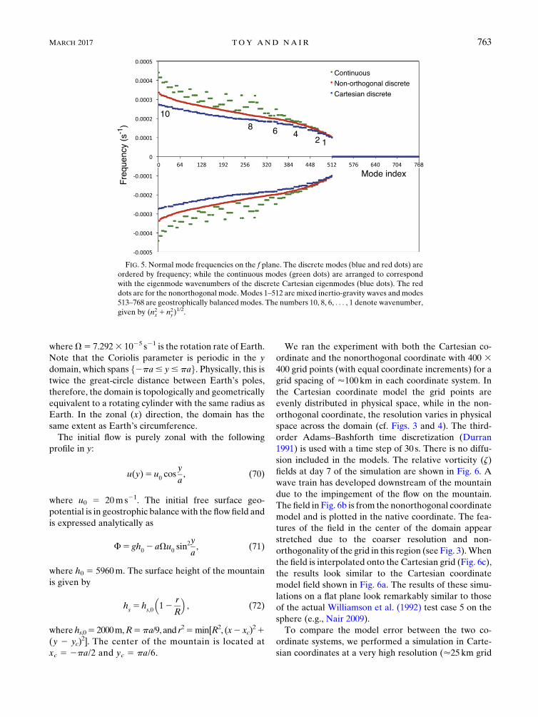
We ran the experiment with both the Cartesian co-ordinate and the nonorthogonal coordinate with 400 3400 grid points (with equal coordinate increments) for agrid spacing of ’100km in each coordinate system. Inthe Cartesian coordinate model the grid points areevenly distributed in physical space, while in the non-orthogonal coordinate, the resolution varies in physicalspace across the domain (cf. Figs. 3 and 4). The third-order Adams–Bashforth time discretization (Durran1991) is used with a time step of 30 s. There is no diffu-sion included in the models. The relative vorticity (z)fields at day 7 of the simulation are shown in Fig. 6. Awave train has developed downstream of the mountaindue to the impingement of the flow on the mountain.The field in Fig. 6b is from the nonorthogonal coordinatemodel and is plotted in the native coordinate. The fea-tures of the field in the center of the domain appearstretched due to the coarser resolution and non-orthogonality of the grid in this region (see Fig. 3).Whenthe field is interpolated onto the Cartesian grid (Fig. 6c),the results look similar to the Cartesian coordinatemodel field shown in Fig. 6a. The results of these simu-lations on a flat plane look remarkably similar to thoseof the actual Williamson et al. (1992) test case 5 on thesphere (e.g., Nair 2009).To compare the model error between the two co-

ordinate systems, we performed a simulation in Carte-sian coordinates at a very high resolution (’25km grid

FIG. 5. Normal mode frequencies on the f plane. The discrete modes (blue and red dots) areordered by frequency; while the continuous modes (green dots) are arranged to correspondwith the eigenmode wavenumbers of the discrete Cartesian eigenmodes (blue dots). The reddots are for the nonorthogonal mode.Modes 1–512 are mixed inertio-gravity waves andmodes513–768 are geostrophically balanced modes. The numbers 10, 8, 6, . . . , 1 denote wavenumber,given by (n2

x 1 n2y)

1/2.


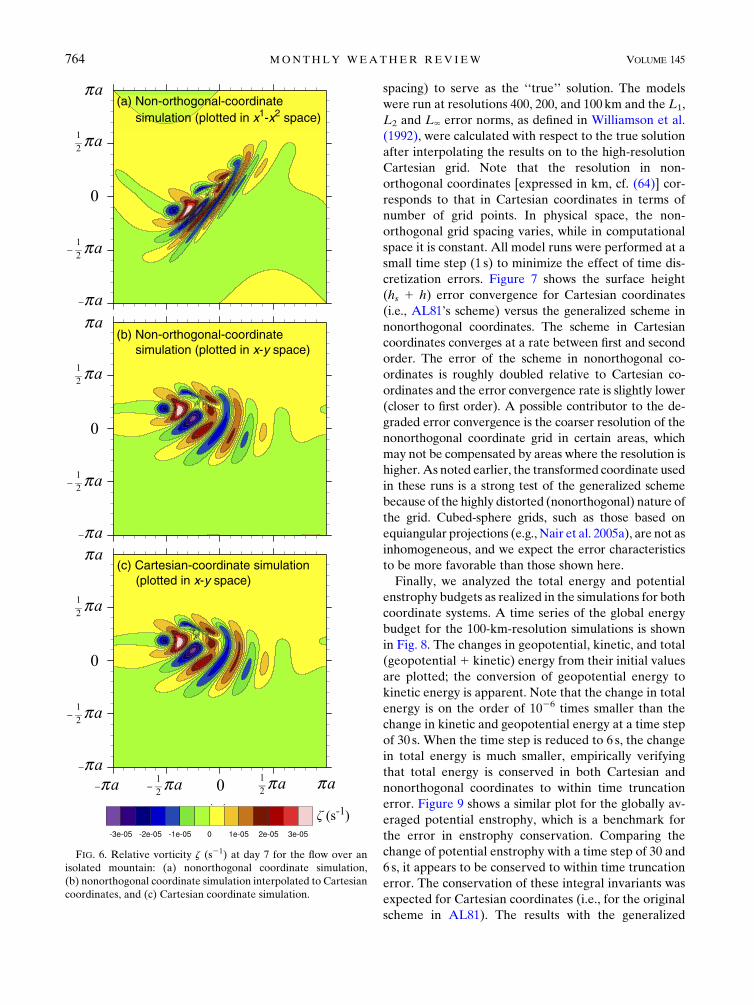
spacing) to serve as the ‘‘true’’ solution. The modelswere run at resolutions 400, 200, and 100 km and the L1,L2 and L‘ error norms, as defined in Williamson et al.(1992), were calculated with respect to the true solutionafter interpolating the results on to the high-resolutionCartesian grid. Note that the resolution in non-orthogonal coordinates [expressed in km, cf. (64)] cor-responds to that in Cartesian coordinates in terms ofnumber of grid points. In physical space, the non-orthogonal grid spacing varies, while in computationalspace it is constant. All model runs were performed at asmall time step (1 s) to minimize the effect of time dis-cretization errors. Figure 7 shows the surface height(hs 1 h) error convergence for Cartesian coordinates(i.e., AL81’s scheme) versus the generalized scheme innonorthogonal coordinates. The scheme in Cartesiancoordinates converges at a rate between first and secondorder. The error of the scheme in nonorthogonal co-ordinates is roughly doubled relative to Cartesian co-ordinates and the error convergence rate is slightly lower(closer to first order). A possible contributor to the de-graded error convergence is the coarser resolution of thenonorthogonal coordinate grid in certain areas, whichmay not be compensated by areas where the resolution ishigher. As noted earlier, the transformed coordinate usedin these runs is a strong test of the generalized schemebecause of the highly distorted (nonorthogonal) nature ofthe grid. Cubed-sphere grids, such as those based onequiangular projections (e.g., Nair et al. 2005a), are not asinhomogeneous, and we expect the error characteristicsto be more favorable than those shown here.Finally, we analyzed the total energy and potential

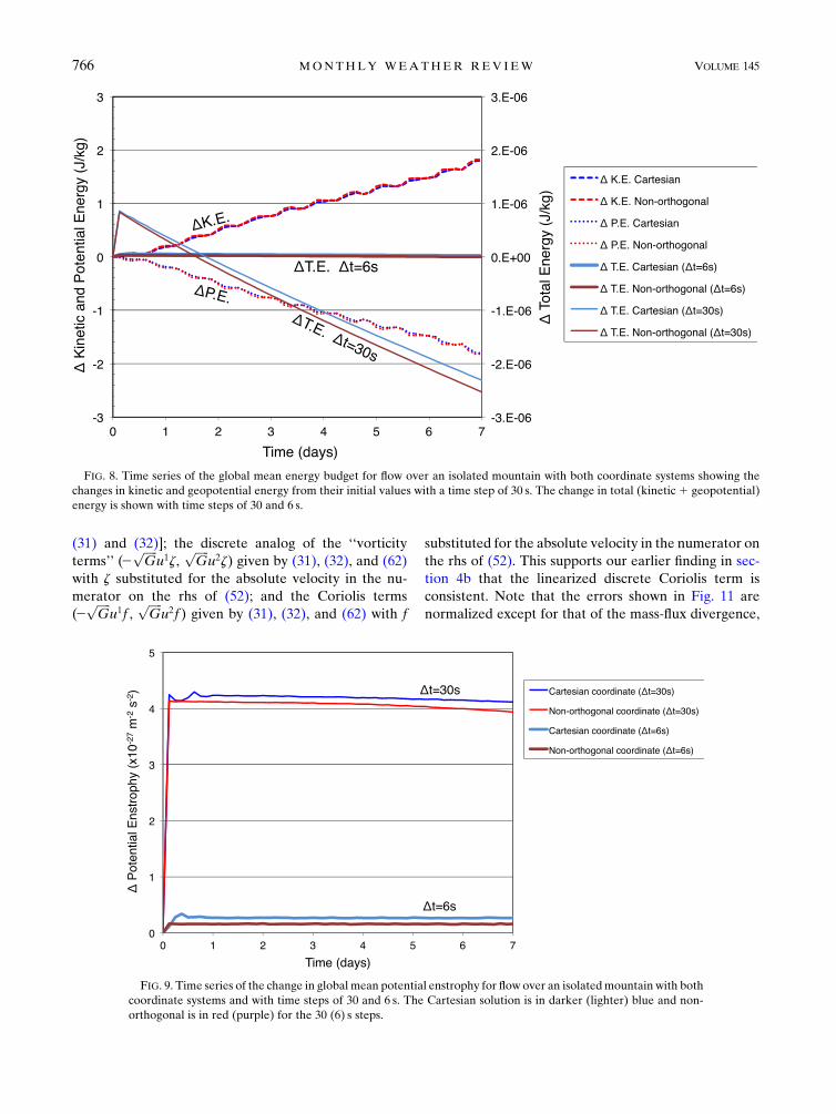
enstrophy budgets as realized in the simulations for bothcoordinate systems. A time series of the global energybudget for the 100-km-resolution simulations is shownin Fig. 8. The changes in geopotential, kinetic, and total(geopotential1 kinetic) energy from their initial valuesare plotted; the conversion of geopotential energy tokinetic energy is apparent. Note that the change in totalenergy is on the order of 1026 times smaller than thechange in kinetic and geopotential energy at a time stepof 30 s. When the time step is reduced to 6 s, the changein total energy is much smaller, empirically verifyingthat total energy is conserved in both Cartesian andnonorthogonal coordinates to within time truncationerror. Figure 9 shows a similar plot for the globally av-eraged potential enstrophy, which is a benchmark forthe error in enstrophy conservation. Comparing thechange of potential enstrophy with a time step of 30 and6 s, it appears to be conserved to within time truncationerror. The conservation of these integral invariants wasexpected for Cartesian coordinates (i.e., for the originalscheme in AL81). The results with the generalized

FIG. 6. Relative vorticity z (s21) at day 7 for the flow over anisolated mountain: (a) nonorthogonal coordinate simulation,(b) nonorthogonal coordinate simulation interpolated to Cartesiancoordinates, and (c) Cartesian coordinate simulation.


curvilinear coordinate verify that the invariants areconserved under the new extended scheme.

d. Steady-state nonlinear zonal geostrophic flow:Analysis of discretization and local truncationerrors

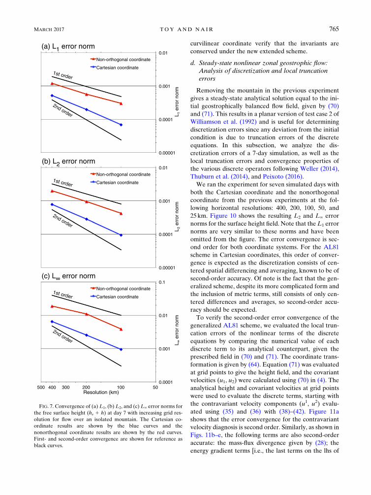
Removing the mountain in the previous experimentgives a steady-state analytical solution equal to the ini-tial geostrophically balanced flow field, given by (70)and (71). This results in a planar version of test case 2 ofWilliamson et al. (1992) and is useful for determiningdiscretization errors since any deviation from the initialcondition is due to truncation errors of the discreteequations. In this subsection, we analyze the dis-cretization errors of a 7-day simulation, as well as thelocal truncation errors and convergence properties ofthe various discrete operators following Weller (2014),Thuburn et al. (2014), and Peixoto (2016).We ran the experiment for seven simulated days with

both the Cartesian coordinate and the nonorthogonalcoordinate from the previous experiments at the fol-lowing horizontal resolutions: 400, 200, 100, 50, and25 km. Figure 10 shows the resulting L2 and L‘ errornorms for the surface height field. Note that theL1 errornorms are very similar to these norms and have beenomitted from the figure. The error convergence is sec-ond order for both coordinate systems. For the AL81scheme in Cartesian coordinates, this order of conver-gence is expected as the discretization consists of cen-tered spatial differencing and averaging, known to be ofsecond-order accuracy. Of note is the fact that the gen-eralized scheme, despite its more complicated form andthe inclusion of metric terms, still consists of only cen-tered differences and averages, so second-order accu-racy should be expected.To verify the second-order error convergence of the

generalized AL81 scheme, we evaluated the local trun-cation errors of the nonlinear terms of the discreteequations by comparing the numerical value of eachdiscrete term to its analytical counterpart, given theprescribed field in (70) and (71). The coordinate trans-formation is given by (64). Equation (71) was evaluatedat grid points to give the height field, and the covariantvelocities (u1, u2) were calculated using (70) in (4). Theanalytical height and covariant velocities at grid pointswere used to evaluate the discrete terms, starting withthe contravariant velocity components (u1, u2) evalu-ated using (35) and (36) with (38)–(42). Figure 11ashows that the error convergence for the contravariantvelocity diagnosis is second order. Similarly, as shown inFigs. 11b–e, the following terms are also second-orderaccurate: the mass-flux divergence given by (28); theenergy gradient terms [i.e., the last terms on the lhs of

FIG. 7. Convergence of (a) L1, (b) L2, and (c) L‘ error norms forthe free surface height (hs 1 h) at day 7 with increasing grid res-olution for flow over an isolated mountain. The Cartesian co-ordinate results are shown by the blue curves and thenonorthogonal coordinate results are shown by the red curves.First- and second-order convergence are shown for reference asblack curves.


(31) and (32)]; the discrete analog of the ‘‘vorticityterms’’ (2

ffiffiffiffiffiG

pu1z,

ffiffiffiffiffiG

pu2z) given by (31), (32), and (62)

with z substituted for the absolute velocity in the nu-merator on the rhs of (52); and the Coriolis terms(2

ffiffiffiffiffiG

pu1f ,

ffiffiffiffiffiG

pu2f ) given by (31), (32), and (62) with f

substituted for the absolute velocity in the numerator onthe rhs of (52). This supports our earlier finding in sec-tion 4b that the linearized discrete Coriolis term isconsistent. Note that the errors shown in Fig. 11 arenormalized except for that of the mass-flux divergence,

FIG. 8. Time series of the global mean energy budget for flow over an isolated mountain with both coordinate systems showing thechanges in kinetic and geopotential energy from their initial values with a time step of 30 s. The change in total (kinetic1 geopotential)energy is shown with time steps of 30 and 6 s.

FIG. 9. Time series of the change in global mean potential enstrophy for flow over an isolatedmountain with bothcoordinate systems and with time steps of 30 and 6 s. The Cartesian solution is in darker (lighter) blue and non-orthogonal is in red (purple) for the 30 (6) s steps.


which is the absolute error due to the analytical di-vergence being zero. Finally, we checked the accuracy ofthe Laplacian operator on a scalar field prescribed byc 5 sin(x/a) cos(y/a), following Thuburn et al. (2014).The continuous and discrete forms of the Laplacianoperator are shown in appendix C. The accuracy issecond order as shown in Fig. 11f, which again is due tothe use of centered differences in the discretization.

5. Summary and discussion

We have extended the AL81 energy and potentialenstrophy conserving finite-difference scheme for theshallow-water equations to generalized curvilinear co-ordinates. This was done using classical tensor analysisand discretizing the vector-invariant form of the

equations of motion in generalized coordinates. The re-sult is a minor addition to the AL81 scheme, required forenergy conservation, which vanishes for rectangularCartesian coordinates. We simulated the divergent flowover an isolatedmountain on a plane surfacewith doubly-periodic boundary conditions using a nonorthogonal co-ordinate; the extended scheme was shown to conserveenergy and potential enstrophy to within time-truncationerror. We compared the resolution-dependent errornorm convergence between runs using Cartesian andnonorthogonal coordinates and found that the rates ofconvergence are comparable (between first and secondorder), although the error was somewhat larger with thenonorthogonal coordinate, presumably due to coarseresolution and lack of orthogonality of coordinate lines incertain areas of the domain.

FIG. 10. As in Fig. 7, but for the steady geostrophically balanced (nomountain) test case and the L1 error norm omitted.


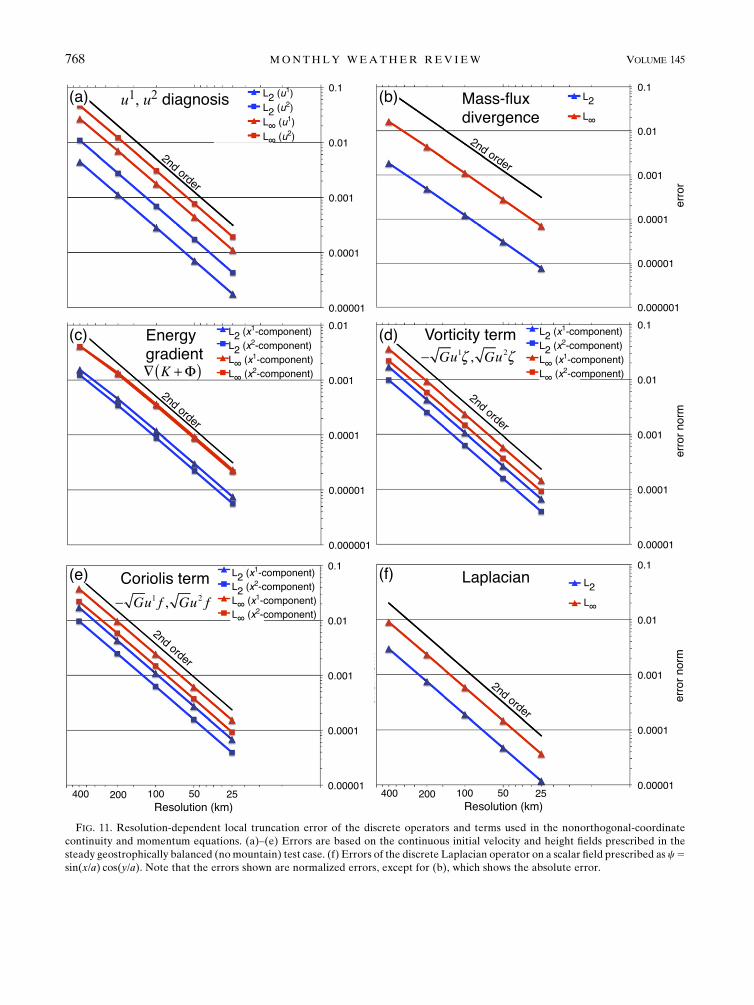
FIG. 11. Resolution-dependent local truncation error of the discrete operators and terms used in the nonorthogonal-coordinatecontinuity and momentum equations. (a)–(e) Errors are based on the continuous initial velocity and height fields prescribed in thesteady geostrophically balanced (nomountain) test case. (f) Errors of the discrete Laplacian operator on a scalar field prescribed as c5sin(x/a) cos(y/a). Note that the errors shown are normalized errors, except for (b), which shows the absolute error.


The AL81 scheme provides a form of the Coriolis termthat does not produce unphysical, nonstationary geostrophicmodes that are sometimes associated with the Arakawa Cgrid staggering (Eldred 2015). Like the original scheme, thenew scheme extended to generalized curvilinear coordinatesprovides a consistent form of the Coriolis term. From anormal mode analysis with the nonorthogonal coordinate, itwas found that the geostrophicmodes remain stationary, thatthere are no unphysical computational modes introduced bythe scheme, and that all of the physicalmodes are stable.Weverified the steadiness of the geostrophic modes by derivingthe discrete linear vorticity equation and checking that fornondivergent flow, the vorticity tendency is zero.The spatial error convergence rates of the nonlinear

discrete terms are formally second order owing the useof centered differencing and averaging, as in the originalAL81 scheme. We verified this empirically by calculat-ing the local truncation error of each term of the modelequations for the geostrophically balanced flow field atvarying grid spacing. The error convergence of the heightfield after a 7-day simulation of the geostrophically bal-anced flow field was also second order.As reported by AL81 and Hollingsworth et al. (1983),

there is a numerical instability (sometimes referred to asthe ‘‘Hollingsworth instability’’) that exists with theAL81scheme when implemented in 3D models. The instabilitycan be avoided by using an alternative form of the dis-crete kinetic energy (e.g., AL81). The result is a loss oftotal energy conservation; however, potential enstrophyis still conserved. We have not yet investigated a stablekinetic energy discretization in generalized curvilinearcoordinates, but it will need to be done before im-plementing the scheme for 3D modeling.The results of the tests show that the generalizedAL81

scheme we have developed could be used advanta-geously in finite-difference global models using cubed-sphere discretizations. A way to obtain the conservationcharacteristics, demonstrated in this paper for interiorgrid points and with periodic boundary conditions, willneed to be developed for the interfaces between the sixregions representing the cube faces; this is left as workfor a forthcoming paper. Also, it may be possible toobtain higher-order accuracy in a generalized-coordinatescheme as was done by Takano and Wurtele (1982) forthe AL81 scheme. Finally, we note that while the

generalized grid we used in the paper was based on amathematically defined coordinate system, as is doneon cubed-sphere grids, the scheme may be used witharbitrary quadrilateral grids, which could be used forrepresenting ocean basins. The elements of the metrictensors would then be determined numerically insteadof analytically. At that point, further analysis will beneeded to determine if the scheme retains second-order accuracy.

Acknowledgments. We would like to thank Drs.Hilary Weller, Pedro Peixoto, Christopher Eldred, andone anonymous reviewer for their helpful and con-structive comments, which greatly improved the paper.The first author would also like to thank the Institute forMathematics Applied to Geosciences (IMAGe) atNCAR for their support and collaboration.

APPENDIX A

Linearized Discrete System of Equations

The continuous system of equations (9)–(11) line-arized about a resting basic state on the f plane can bewritten as

›h

›t1

h0ffiffiffiffiffiG

p$›

›x1(

ffiffiffiffiffiG

pu1)1

›

›x2(

ffiffiffiffiffiG

pu2)

%5 0, (A1)

›u1

›t52g

›h

›x11

ffiffiffiffiffiG

ph0u2q , (A2)

and

›u2

›t52g

›h

›x22

ffiffiffiffiffiG

ph0u1q , (A3)

where h, u1, and u2 refer to perturbation values and q isthe basic-state potential vorticity given by

q5f

h0

. (A4)

Applying the finite-difference scheme derived in section3, the corresponding linearized discrete system sim-plifies to

›

›t(h)

i11/2,j11/2 52h0

d

1

(ffiffiffiffiffiG

p)i11/2,j11/2

[(ffiffiffiffiffiG

p)i

i11,j11/2(u1)


p)i

i,j11/2(u1)

i,j11/2

1 (ffiffiffiffiffiG

p)j

i11/2,j11(u2)


p)j

i11/2,j(u2)

i11/2,j], (A5)


›

›t(u

1)i,j11/252

g

d(h

i11/2,j11/2 2 hi21/2,j11/2)1

f

4[(

ffiffiffiffiffiG

p)j

i11/2,j11(u2)

i11/2,j111 (

ffiffiffiffiffiG

p)j

i21/2,j11(u2)

i21/2,j11

1 (ffiffiffiffiffiG

p)j

i21/2,j(u2)


p)j

i11/2,j(u2)

i11/2,j], (A6)

and

›

›t(u2)i11/2,j52

g

d(h

i11/2,j11/2 2 hi11/2,j21/2)2

f

4[(

ffiffiffiffiffiG

p)i

i11,j11/2(u1)

i11,j11/2 1 (ffiffiffiffiffiG

p)i

i,j11/2(u1)

i,j11/2

1 (ffiffiffiffiffiG

p)i

i,j21/2(u1)

i,j21/2 1 (ffiffiffiffiffiG

p)i

i11,j21/2(u1)

i11,j21/2], (A7)

where

(u1)i,j11/2 5 (G11)

i,j11/2(u1)i,j11/21

1

4

2

664(G12)i,j11/2(G

12)i21/2,j11

ffiffiffiffiffiffiffiffiffiffiffiffiffiffiffiffiffiffiffiffiffiffiffiffiffiffi(

ffiffiffiffiffiG

p)j

i21/2,j11

(ffiffiffiffiffiG

p)i

i,j11/2

vuuut (u2)i21/2,j11

1 (G12)i,j11/2(G

12)i11/2,j11


ffiffiffiffiffiG

p)j

i11/2,j11

(ffiffiffiffiffiG

p)i

i,j11/2

vuuut (u2)i11/2,j111 (G12)i,j11/2(G

12)i21/2,j

ffiffiffiffiffiffiffiffiffiffiffiffiffiffiffiffiffiffiffiffiffiffi(

ffiffiffiffiffiG

p)j

i21/2,j

(ffiffiffiffiffiG

p)i

i,j11/2

vuuut (u2)i21/2,j

1 (G12)i,j11/2(G

12)i11/2,j


ffiffiffiffiffiG

p)j

i11/2,j

(ffiffiffiffiffiG

p)i

i,j11/2

vuuut (u2)i11/2,j

3

775,

(A8)

and

(u2)i11/2,j 5 (G22)

i11/2,j(u2)i11/2,j1

1

4

2

664(G12)i11/2,j(G

12)i,j11/2


ffiffiffiffiffiG

p)i

i,j11/2

(ffiffiffiffiffiG

p)j

i11/2,j

vuuut (u1)i,j11/2

1 (G12)i11/2,j(G

12)i11,j11/2


ffiffiffiffiffiG

p)i

i11,j11/2

(ffiffiffiffiffiG

p)j

i11/2,j

vuuut (u1)i11,j11/2 1 (G12)

i11/2,j(G12)

i,j21/2


ffiffiffiffiffiG

p)i

i,j21/2

(ffiffiffiffiffiG

p)j

i11/2,j

vuuut (u1)i,j21/2

1 (G12)i11/2,j(G

12)i11,j21/2


ffiffiffiffiffiG

p)i

i11,j21/2

(ffiffiffiffiffiG

p)j

i11/2,j

vuuut (u1)i11,j21/2

3

775.

(A9)

APPENDIX B

Linearized Vorticity and Continuity Equationsat q Points

To support the result of our numerical eigendecompo-sition that the generalized AL81 scheme has stationary

geostrophic modes, we derive the linearized discretevorticity equation and show that for geostrophicmodes, inwhich the divergence vanishes, the vorticity tendency alsovanishes (e.g., Thuburn et al. 2009). The time tendency ofthe perturbation relative vorticity zi,j from a resting basicstate on the f plane can be obtained by using (52) and (54)in (56) combined with (62) and (A4) to give


›

›t(

ffiffiffiffiffiG

pz)

i,j 52f

4d[(

ffiffiffiffiffiG

pu2)

i11/2,j112 (

ffiffiffiffiffiG

pu2)

i11/2,j211 (

ffiffiffiffiffiG

pu2)

i21/2,j112 (

ffiffiffiffiffiG

pu2)

i21/2,j21

1 (ffiffiffiffiffiG

pu1)


pu1)


pu1)


pu1)

i21,j21/2], (B1)

where u1 and u1 are the perturbation contravariant ve-locity components. Note that the basic-state fluid depth

h0 has cancelled out. The linearized continuity equationat vorticity points is readily obtained from (58) as

›

›t(

ffiffiffiffiffiG

ph)

(q)

i,j 52h0

4d[(

ffiffiffiffiffiG

pu2)


pu2)

i11/2,j21 1 (ffiffiffiffiffiG

pu2)


pu2)

i21/2,j21

1 (ffiffiffiffiffiG

pu1)


pu1)


pu1)


pu1)

i21,j21/2]. (B2)

When the flow is nondivergent as seen by the fluid depthat mass points, the rhs of (B2) vanishes (i.e., the flow isalso nondivergent in terms of continuity at the vorticitypoints). Therefore, the rhs of (B1) is zero, which confirmsthat the nondivergent geostrophic modes are steady.

APPENDIX C

The Laplacian Operator

The Laplacian operator expressed in generalized curvi-linear coordinates (e.g.,Nair 2009) canbewritten as follows:

=2c51ffiffiffiffiffiG

p$›

›x1

! ffiffiffiffiffiG

pG11 ›c

›x1

"1

›

›x1

! ffiffiffiffiffiG

pG12 ›c

›x2

"

1›

›x2

! ffiffiffiffiffiG

pG21 ›c

›x1

"1

›

›x2

! ffiffiffiffiffiG

pG22 ›c

›x2

"%,

(C1)

where c is a scalar. The discrete form of (C1) used in thetruncation error analysis of section 4d is given by

(=2c)i11/2,j11/2 5

1

d2(ffiffiffiffiffiG

p)i11/2,j11/2

f[(ffiffiffiffiffiG

pG11)

i11(ci13/2 2ci11/2)2 (

ffiffiffiffiffiG

pG11)

i(c

i11/2 2ci21/2)]j11/2


pG12)

i11,j11/2(ci11,j11 2ci11,j)2 (

ffiffiffiffiffiG

pG12)

i,j11/2(ci,j11 2ci,,j)]


pG21)

i11/2,j11(ci11,j11 2ci,j11)2 (

ffiffiffiffiffiG

pG21)

i11/2,j(ci11,j 2ci,j)]


pG22)

j11(cj13/2 2cj11/2)2 (

ffiffiffiffiffiG

pG22)

j(c

j11/2 2cj21/2)]i11/2g . (C2)

REFERENCES

Adcroft, A., J.-M. Campin, C. Hill, and J. Marshall, 2004: Im-

plementation of an atmosphere–ocean general circulation

model on the expanded spherical cube. Mon. Wea. Rev., 132,2845–2863, doi:10.1175/MWR2823.1.

Arakawa, A., and V. R. Lamb, 1977: Computational design of the

basic dynamical process of the UCLA general circulation

model.Methods in Computational Physics, J. Chang, Ed., Vol.

17, Academic Press, 173–265.——, and ——, 1981: A potential enstrophy and energy con-

serving scheme for the shallow water equations.Mon. Wea.

Rev., 109, 18–36, doi:10.1175/1520-0493(1981)109,0018:

APEAEC.2.0.CO;2.Bao, L., R. D. Nair, and H. M. Tufo, 2014: A mass and momentum

flux-form high-order discontinuous Galerkin shallow water

model on the cubed-sphere. J. Comput. Phys., 271, 224–243,

doi:10.1016/j.jcp.2013.11.033.Bleck, R., and Coauthors, 2015: A vertically flow-following icosa-

hedral grid model for medium-range and seasonal prediction.

Part I: Model description. Mon. Wea. Rev., 143, 2386–2403,doi:10.1175/MWR-D-14-00300.1.

Bonaventura, L., and T. Ringler, 2005: Analysis of discrete shallow-water models on geodesic Delaunay grids with C-type staggering.Mon. Wea. Rev., 133, 2351–2373, doi:10.1175/MWR2986.1.

Durran, D. R., 1991: The third-order Adams–Bashforth method:An attractive alternative to leapfrog time differencing. Mon.Wea. Rev., 119, 702–720, doi:10.1175/1520-0493(1991)119,0702:TTOABM.2.0.CO;2.

Dutton, J. A., 1986: The Ceaseless Wind: An Introduction to the

Theory of Atmospheric Motion. Dover Publications, 617 pp.Eldred, C., 2015: Linear and nonlinear properties of numerical

methods for the rotating shallow water equations. Ph.D.thesis, Colorado State University, 274 pp. [Available onlineat http://hdl.handle.net/10217/167080.]

Gassmann, A., 2011: Inspection of hexagonal and triangular C-griddiscretizations of the shallow water equations. J. Comput.Phys., 230, 2706–2721, doi:10.1016/j.jcp.2011.01.014.

Heikes, R., and D. A. Randall, 1995a: Numerical integration of theshallow-water equations on a twisted icosahedral grid. Part I:


http://dx.doi.org/10.1175/MWR2823.1

http://dx.doi.org/10.1016/j.jcp.2013.11.033

http://dx.doi.org/10.1175/MWR-D-14-00300.1


http://hdl.handle.net/10217/167080


Basic design and results of tests.Mon.Wea. Rev., 123, 1862–1880,doi:10.1175/1520-0493(1995)123,1862:NIOTSW.2.0.CO;2.

——, and ——, 1995b: Numerical integration of the shallow-waterequations on a twisted icosahedral grid. Part II: A detailed de-scription of the grid and an analysis of numerical accuracy.Mon.Wea.Rev., 123, 1881–1887, doi:10.1175/1520-0493(1995)123,1881:NIOTSW.2.0.CO;2.

Hirani, A. N., 2003: Discrete exterior calculus. Ph.D. thesis, Cal-ifornia Institute of Technology, 103 pp. [Available online athttp://thesis.library.caltech.edu/1885/3/thesis_hirani.pdf.]

Hollingsworth, A., P. Kållberg, V. Renner, and D. M. Burridge,1983: An internal symmetric computational instability. Quart.J. Roy. Meteor. Soc., 109, 417–428, doi:10.1002/qj.49710946012.

Lee, J.-L., and A. E. MacDonald, 2009: A finite-volume icosahe-dral shallow-water model on a local coordinate. Mon. Wea.Rev., 137, 1422–1437, doi:10.1175/2008MWR2639.1.

McGregor, J. L., 1996: Semi-Lagrangian advection on conformal-cubic grids. Mon. Wea. Rev., 124, 1311–1322, doi:10.1175/1520-0493(1996)124,1311:SLAOCC.2.0.CO;2.

Nair, R. D., 2009: Diffusion experiments with a global discontin-uous Galerkin shallow-water model. Mon. Wea. Rev., 137,3339–3350, doi:10.1175/2009MWR2843.1.

——, S. J. Thomas, and R. D. Loft, 2005a: A discontinuous Galerkinglobal shallow water model. Mon. Wea. Rev., 133, 876–888,doi:10.1175/MWR2903.1.

——, ——, and ——, 2005b: A discontinuous Galerkin transportscheme on the cubed sphere. Mon. Wea. Rev., 133, 814–828,doi:10.1175/MWR2890.1.

Peixoto, P. S., 2016: Accuracy analysis of mimetic finite volumeoperators on geodesic grids and a consistent alternative. J.Comput.Phys., 310, 127–160, doi:10.1016/j.jcp.2015.12.058.

Ran!cic, M., R. J. Purser, and F. Mesinger, 1996: A global shallow-water model using an expanded spherical cube: Gnomonicversus conformal coordinates.Quart. J. Roy.Meteor. Soc., 122,959–982, doi:10.1002/qj.49712253209.

Randall, D. A., 1994: Geostrophic adjustment and the finite-differenceshallow-water equations. Mon. Wea. Rev., 122, 1371–1377,doi:10.1175/1520-0493(1994)122,1371:GAATFD.2.0.CO;2.

Ringler, T. D., and D. A. Randall, 2002: A potential enstrophy andenergy conserving numerical scheme for solution of the shallow-water equations on a geodesic grid. Mon. Wea. Rev., 130, 1397–1410, doi:10.1175/1520-0493(2002)130,1397:APEAEC.2.0.CO;2.

——, J. Thuburn, J. B. Klemp, and W. C. Skamarock, 2010: Aunified approach to energy conservation and potential vor-ticity dynamics for arbitrarily-structured C-grids. J. Comput.Phys., 229, 3065–3090, doi:10.1016/j.jcp.2009.12.007.

Ronchi, C., R. Iacono, and P. S. Paolucci, 1996: The ‘‘cubedsphere’’: A new method for the solution of partial differentialequations in spherical geometry. J. Comput. Phys., 124, 93–114,doi:10.1006/jcph.1996.0047.

Sadourny, R., 1972: Conservative finite-difference approximationsof the primitive equations on quasi-uniform spherical grids.Mon.Wea. Rev., 100, 136–144, doi:10.1175/1520-0493(1972)100,0136:CFAOTP.2.3.CO;2.

——, A. Arakawa, and Y. Mintz, 1968: Integration of the non-divergent barotropic vorticity equation with an icosahedral-hexagonal grid for the sphere. Mon. Wea. Rev., 96, 351–356,doi:10.1175/1520-0493(1968)096,0351:IOTNBV.2.0.CO;2.

Salmon, R., 2004: Poisson-bracket approach to the construction ofenergy- and potential-enstrophy-conserving algorithms for theshallow-water equations. J. Atmos. Sci., 61, 2016–2036, doi:10.1175/1520-0469(2004)061,2016:PATTCO.2.0.CO;2.

——, 2007: A general method for conserving energy and potentialenstrophy in shallow-watermodels. J. Atmos. Sci., 64, 515–531,doi:10.1175/JAS3837.1.

Satoh,M., T. Matsuno, H. Tomita, H.Miura, T. Nasuno, and S. Iga,2008: Nonhydrostatic icosahedral atmospheric model (NICAM)for global cloud resolving simulations. J. Comput. Phys., 227,3486–3514, doi:10.1016/j.jcp.2007.02.006.

Stuhne, G. R., and W. R. Peltier, 2006: A robust unstructured griddiscretization for 3-dimensional hydrostatic flows in sphericalgeometry: A new numerical structure for ocean general cir-culation modeling. J. Comput. Phys., 213, 704–729, doi:10.1016/j.jcp.2005.08.031.

Takano, K., and M. G. Wurtele, 1982: A fourth-order energy andpotential enstrophy conserving difference scheme. Tech. Rep.AFGL-TR-82-0205, Air Force Geophysics Laboratory, 85 pp.

Thuburn, J., 2008: Numerical wave propagation on the hexago-nal C-grid. J. Comput. Phys., 227, 5836–5858, doi:10.1016/j.jcp.2008.02.010.

——, and C. J. Cotter, 2012: A framework for mimetic discretization ofthe rotating shallow-water equations on arbitrary polygonal grids.SIAM J. Sci. Comput., 34, B203–B225, doi:10.1137/110850293.

——, T. D. Ringler, W. C. Skamarock, and J. B. Klemp, 2009:Numerical representation of geostrophic modes on arbitrarilystructured C-grids. J. Comput. Phys., 228, 8321–8335, doi:10.1016/j.jcp.2009.08.006.

——, C. J. Cotter, and T. Dubos, 2014: A mimetic, semi-implicit,forward-in-time, finite volume shallow water model: Compari-son of hexagonal-icosahedral and cubed-sphere grids. Geosci.Model Dev., 7, 909–929, doi:10.5194/gmd-7-909-2014.

Tort, M., T. Dubos, and T. Melvin, 2015: Energy-conserving finite-difference schemes for quasi-hydrostatic equations. Quart.J. Roy. Meteor. Soc., 141, 3056–3075, doi:10.1002/qj.2590.

Warsi, Z. U. A., 2006: Fluid Dynamics: Theoretical and Compu-tational Approaches. 3rd ed. CRC Press, 872 pp.

Weller, H., 2014: Non-orthogonal version of the arbitrary polygo-nal C-grid and a new diamond grid. Geosci. Model Dev., 7,779–797, doi:10.5194/gmd-7-779-2014.

Wesseling, P., 2009: Principles of Computational Fluid Dynamics.Springer-Verlag, 644 pp.

Williamson, D. L., 1968: Integration of the barotropic vorticityequation on a spherical geodesic grid. Tellus, 20A, 642–653,doi:10.1111/j.2153-3490.1968.tb00406.x.

——, J. B. Drake, J. J. Hack, R. Jakob, and P. N. Swarztrauber,1992: A standard test set for numerical approximations to theshallow water equations in spherical geometry. J. Comput.Phys., 102, 211–224, doi:10.1016/S0021-9991(05)80016-6.


http://thesis.library.caltech.edu/1885/3/thesis_hirani.pdf

http://dx.doi.org/10.1002/qj.49710946012

http://dx.doi.org/10.1175/2008MWR2639.1

http://dx.doi.org/10.1175/2009MWR2843.1




http://dx.doi.org/10.1002/qj.49712253209


http://dx.doi.org/10.1006/jcph.1996.0047

http://dx.doi.org/10.1175/JAS3837.1






http://dx.doi.org/10.1137/110850293



http://dx.doi.org/10.5194/gmd-7-909-2014

http://dx.doi.org/10.1002/qj.2590

http://dx.doi.org/10.5194/gmd-7-779-2014

http://dx.doi.org/10.1111/j.2153-3490.1968.tb00406.x

http://dx.doi.org/10.1016/S0021-9991(05)80016-6

Documents

A Potential Enstrophy and Energy Conserving Scheme … Potential Enstrophy and Energy Conserving Scheme for the Shallow-Water Equations Extended to Generalized Curvilinear Coordinates