Embed Size (px)
Citation preview
A Possible Link between the Electroweak
Phase Transition and the Dark Matter of the
Universe
Thesis submitted for the degree ofDoctor of Philosophy
Candidate: Supervisor:Talal Ahmed Chowdhury Prof. Goran Senjanovic
Theoretical Particle PhysicsScuola Internazionale Superiore di Studi Avanzati-SISSA
Trieste, ItalySeptember, 2014
Abstract
A possible connection between the dark matter and strong first order elec-troweak phase transition, which is an essential ingredient of the electroweakbaryogenesis, has been explored in this thesis. It is shown that the extensionof the Standard Model’s minimal Higgs sector with an inert SU(2)L scalardoublet can provide light dark matter candidate and simultaneously inducea strong first order phase transition. There is however no symmetry reasonto prevent the extension using scalars with higher SU(2)L representations.Therefore, by making random scans over the models’ parameters, we show,in the light of electroweak physics constraints, strong first order electroweakphase transition and the possibility of having a sub-TeV cold dark mattercandidate, that the higher representations are rather disfavored comparedto the inert doublet. This is done by computing generic perturbativity be-havior and impact on electroweak phase transitions of higher representationsin comparison with the inert doublet model. Explicit phase transition andcold dark matter phenomenology within the context of the inert triplet andquartet representations are used for detailed illustrations.
Acknowledgements
I am deeply indebted to my supervisor Prof. Goran Senjanovic for his guid-ance in every step of my research. My sincerest gratitude to him for histeaching and supervision since the ICTP diploma course and for the free-dom he has given me to pursue and find my ways. I have greatly benefitednot only from his deep insight of physics but also from his advice regardingphysics and life. His words and guidance will always be one of the mostvaluable lessons in my life.
My sincerest gratitude to Prof. Jim Cline and Prof. Fabrizio Nesti fortheir careful considerations on the thesis and giving important suggestions.
I am grateful to Prof. Roberto Iengo, Prof. Serguey Petcov, Prof. MarcoSerone, Prof. Matteo Bertolini, Prof. Andrea Romanino, Prof. Andrea DeSimone, Prof. Piero Ullio, Prof. Stefano Liberati, Prof. Giulio Bonelli,Prof. Loriano Bonora, Prof. Guido Martinelli and Prof. Marco Fabbrich-esi for teaching me advanced topics of high energy physics during my PhDcoursework in SISSA.
I am also grateful to Prof. Seifallah Randjbar-Daemi, Prof. Edi Gava,Prof. Bobby Acharya, Prof. Alexei Smirnov, Prof. Kumar Narain and Prof.Paolo Creminelli for helping me build up the foundation with their teach-ings in ICTP’s high energy physics diploma course. I am thankful to KerimSuruliz, Mahdi Torabian, T. Enkhbat, Aseem Paranjape, Koji Tsumura andEnrico Trincherini for enjoyable tutorials during the course. I am also thank-ful to Prof. George Thompson and Prof. Giovanni Villadoro.
My special thanks to Prof. Arshad Momen, Prof. Kamrul Hassan, Prof,Khorshed Ahmed Kabir, Prof. Golam Mohammad Bhuiyan and Dr. MahbubMajumder for the guidance during my undergraduate studies in Universityof Dhaka.
I am thankful to Prof. A. M. Harun-Ar-Rashid and late Prof. JamalNazrul Islam for the giving me the inspiration to pursue physics from thevery early stage in my life.
I am grateful to Yue Zhang, Miha Nemevsek, Shehu S. AbdusSalam,Amine Ahriche, Salah Nasri and Rachik Soualah for the collaboration andgiving me the opportunity to learn in the process.
I am indebted to Basudeb Dasgupta for his advice and suggestions onresearch and Xiaoyong Chu for numerous discussions on various topics ofphysics and life. I am also grateful to Rajesh Kumar Gupta and GabrijelaZaharijas for many discussions. My special thanks to Ehsan Hatefi, EmilianoSefusatti, Diana Lopez Nacir and Kate Shaw.
My heartfelt gratitude to my friends and classmates: Marko, Emanuele,Gabriele, Nouman, Alejandro, Alberto, Piermarco, David, Carlo, Marco,
1
Lorezo, Flavio, Eolo, Pietro and Claudia. My special thanks to Luca DiLuzio, Marco Nardecchia and Aurora Meroni. I am also thankful to myclassmates from the diploma course; and my seniors, classmates and juniorsfrom University of Dhaka. Also thanks to my friends scattered all over theworld for their continuous support.
I am grateful to Prof. Rohini Godbole, Prof. Dilip Kumar Ghosh andProf. Sunil Mukhi for the advice, encouragement and collaboration. I amthankful to Prof. Syed Twareque Ali and Prof. Jean Pierre Gazeau for theadvice and collaboration. I am greatly indebted to Prof. Fernando Quevedofor his support, advice and encouragement.
I am also grateful to Riccardo, Federica, Barbara and Rosanna for helpingme completing all the administrative requirements.
I am thankful to Gabriele, Lucina, Adriano, Angie, Rosie, Maria andGuendalina for giving me the warmth of a family. My thanks to Nicoletta,Natalia and Ettore for the kindness and support. Also a special thanks tothe members of Manoaperta for the exciting moments.
My special thanks to Anamika.Last but not least, I want to thank my family for everything they have
done for me. This thesis is dedicated to my mother and to the memory ofmy father.
2
Contents
1 Introduction 6
2 Elements of finite temperature field theory 102.1 Thermodynamic quantities . . . . . . . . . . . . . . . . . . . . 102.2 Tools of finite temperature field theory . . . . . . . . . . . . . 14
2.2.1 Imaginary time formalism . . . . . . . . . . . . . . . . 152.2.2 A toy model at finite temperature . . . . . . . . . . . . 19
2.3 Effective potential at finite temperature . . . . . . . . . . . . . 222.3.1 Effective potential as the sum of 1PI digrams . . . . . 232.3.2 Effective potential from the path integral . . . . . . . . 252.3.3 Effective potential for scalar, fermion and vector fields 272.3.4 Finite temperature effective potential . . . . . . . . . . 29
2.4 Phase transition in the early universe . . . . . . . . . . . . . . 352.4.1 First and second order phase transitions . . . . . . . . 362.4.2 Electroweak phase transition in the Standard Model . . 38
2.5 Infrared problems and resummation . . . . . . . . . . . . . . . 402.5.1 The scalar theory . . . . . . . . . . . . . . . . . . . . . 432.5.2 The Standard Model . . . . . . . . . . . . . . . . . . . 44
3 Electroweak Baryogenesis: the need for strong phase transi-tion 463.1 Sakharov’s conditions for baryogenesis . . . . . . . . . . . . . 473.2 Electroweak baryogenesis . . . . . . . . . . . . . . . . . . . . . 493.3 Baryon number violation at finite temperature by the sphaleron 54
3.3.1 Sphaleron in SU(2)L scalar representation . . . . . . . 553.3.2 Baryon number violation at T > Tc and T < Tc . . . . 603.3.3 Sphaleron decoupling and the strong EWPhT condition 62
4 Scalar representations in the light of electroweak phase tran-sition and cold dark matter phenomenology 654.1 Scalar representations beyond the Standard Model . . . . . . . 66
3
4.1.1 Scalar multiplets with cold dark matter candidates . . 664.1.2 Inert Doublet, Triplet and Quartet mass spectra . . . . 674.1.3 Perturbativity and EW physics constraints on the size
of the multiplets . . . . . . . . . . . . . . . . . . . . . 724.2 Electroweak phase transition (EWPhT) . . . . . . . . . . . . . 77
4.2.1 Finite temperature effective potential . . . . . . . . . . 774.2.2 EWPhT with the Inert Doublet, Triplet and Quartet
representations . . . . . . . . . . . . . . . . . . . . . . 794.2.3 Impact of multiplets’ sizes on EWPhT . . . . . . . . . 89
4.3 Interplay between EWPhT and CDM constraints in the InertDoublet . . . . . . . . . . . . . . . . . . . . . . . . . . . . . . 914.3.1 The inert doublet as dark matter . . . . . . . . . . . . 914.3.2 Interplay between EWPhT and CDM constraints . . . 92
4.4 The Quartet/Doublet versus EW, EWPhT and CDM con-straints. . . . . . . . . . . . . . . . . . . . . . . . . . . . . . . 944.4.1 Model parameters scan and constraints . . . . . . . . . 944.4.2 Allowed parameter regions . . . . . . . . . . . . . . . . 96
4.5 Summary . . . . . . . . . . . . . . . . . . . . . . . . . . . . . 98
5 Conclusions and outlook 99
A Mathematical tools 103A.1 Properties of Γ(s) and ζ(s) . . . . . . . . . . . . . . . . . . . . 103A.2 Some useful integrals . . . . . . . . . . . . . . . . . . . . . . . 104A.3 Frequency sum . . . . . . . . . . . . . . . . . . . . . . . . . . 105
B Coleman-Weinberg potential 107B.1 MS renormalization . . . . . . . . . . . . . . . . . . . . . . . 107B.2 CW effective potential in the Standard Model . . . . . . . . . 108
B.2.1 MS renormalization . . . . . . . . . . . . . . . . . . . . 109B.2.2 Cut-off regularization . . . . . . . . . . . . . . . . . . . 109
C High and low temperature expansion 110C.1 Limits of thermodynamic quantities . . . . . . . . . . . . . . . 110C.2 High temperature expansion for the toy model . . . . . . . . . 113C.3 High and low temperature expansion of the effective potential 114
C.3.1 Bosonic high temperature expansion . . . . . . . . . . 114C.3.2 Fermionic high temperature expansion . . . . . . . . . 117C.3.3 Low temperature expansion . . . . . . . . . . . . . . . 119
D Asymptotic limits of the sphaleron field profiles 120
4

E Quartet SU(2) representation 123E.1 SU(2) generators in the quartet . . . . . . . . . . . . . . . . . 123E.2 Gauge-scalar-scalar vertices . . . . . . . . . . . . . . . . . . . 124
F Tree-Unitarity 125
G Renormalization group equations 129
5
Chapter 1
Introduction
The discovery of an about 126 GeV Higgs boson [1, 2] is yet another im-portant support for and completion of the Standard Model (SM). The SMwith minimal Higgs sector contains one complex Higgs doublet which afterelectroweak symmetry breaking gives a neutral CP-even Higgs boson. Butone can consider a scenario with singlets, with more than one doublet or withan N copies of SU(2)L n-tuplets where the (non standard) Higgs sector canbe used to explicitly account for Baryogenesis and cold dark matter. Usingthese phenomena and related experimental data we set to qualitatively ex-plore for the preferred scalar representation in the SM.
Extensive astrophysical and cosmological observations have already putdark matter (DM) as a constituent of the universe. The existence of DMhas been indicated by the rotation curves for spiral galaxies [3], velocity dis-persion of individual galaxies in galaxy clusters, large x-ray temperatures ofclusters [4], bulk flows and the peculiar motion of our own local group [5],Moreover, inferred from the gravitational lensing of background images, themass of galaxy clusters turn out to be consistent with the large dark-to-visible mass ratios [6]. Furthermore, one of the most compelling evidence, ata statistical significance of 8σ comes from the two colliding clusters of galax-ies, known as the Bullet cluster [7] for which the spatial displacement of thecenter of the total mass from the center of the baryonic mass peaks cannotbe explained with an alteration of gravitational force law. Also, the largescale structure formation from the initial seed perturbations from inflationrequires a significant non-baryonic dark matter component [8]. Finally theobserved acoustic peaks in the cosmic microwave background radiation en-ables us to determine most precisely the relic density of DM in the universeto be, ΩDMh
2 = 0.1196 ± 0.0031 (68% CL) [9] as the DM density providesthe required potential well for the observed acoustic oscillation seen in the
6
CMB. Still we have to determine the exact nature of the dark matter fromparticle physics point of view. Within many viable candidates for DM, themost popular one is considered to be the stable weakly interacting particle(WIMP) [10] for which the observed DM relic density is obtained if it’s masslies near the electroweak scale.
Apart from DM identification, one other unresolved question within theSM is the observed matter-antimatter asymmetry of the universe. Such asym-metry is described by Baryogenesis scenario first put forward by Sakharov [11]and one essential ingredient of this mechanism is ’out of equilibrium process’.Now that the study of beyond standard model (BSM) physics is being ex-plored with the LHC, a well motivated scenario within the testable reach ofLHC is Electroweak Baryogenesis [12] where out of equilibrium condition isgiven by strong first order phase transition. The SM has all the tools requiredby the Sakharov’s condition for Baryogenesis, i.e. baryon number violationat high temperature through sphalerons [13–16], C and CP violation withCKM phase and strong first order phase transition [17, 18]. However, it wasshown that to avoid baryon washout by sphalerons, Higgs mass has to be be-low 45 GeV for strong electroweak phase transition (EWPhT) [19–22], whichwas later confirmed by lattice studies [23–25] and eventually it was ruled outby the LEP data [26]. Now with Higgs at 126 GeV, clearly one can see therequirement of extending SM by new particles, possibly lying nearly the elec-troweak scale, which could not only provide strong EWPhT for explainingmatter asymmetry but also the DM content of the universe.
One promising way is to extend the scalar sector of the SM. Within theliterature there are numerous considerations for non minimal Higgs sectorwith various representations of the additional Higgs multiplet in order to ac-count for Baryogenesis and/or dark matter. For instance, in the inert doubletcase considered in [27–29], it was shown that it can enable one to achievestrong EWPhT with DM mass lying between 45 GeV and 80 GeV and pre-dicts a lower bound on the direct detection that is consistent with XENONdirect detection limit [208] (in case of sub-dominant DM, see [30]). Inertdoublet is a well motivated and minimal extension of scalar sector whichwas first proposed as dark matter [31], was studied as a model for radiativeneutrino mass generation [32], improved naturalness [33] and follows natu-rally [34, 35] in case of mirror families [36–39] that was to fulfill Lee andYang’s dream to restore parity [40]. The DM phenomenology regarding In-ert doublet model has been studied extensively in Refs. [41–55]. Moreover,tentative 130 GeV gamma line from galactic center can be accommodated ininert doublet framework [57]. Therefore, one can extend scalar sector by in-
7
troducing inert scalar representations and explore the nature of phase transi-tion, consistency of the theory at high scale and dark matter phenomenology.
Apart from the doublet, one other possibility is the scalar singlet [58–62](and references there) which can be accounted for strong EWPhT and lightDM candidate but not simultaneously (for exceptions, see [63–65]). Scalarsinglet can also be a force carrier between SM and dark matter sector induc-ing strong EWPhT [66,67] or trigger EWPhT independent of being DM [68].
In the case of larger representations, a systematic study for DM candi-date has been performed in [69] from doublet to 7-plet of SU(2)L with bothfermionic and scalar DM where only allowed interactions of DM are gauge in-teractions. Additionally, scalar multiplet allows renormalizable quartic cou-plings with Higgs doublet. In [70], study of DM phenomenology for suchscalar multiplet was carried out for large odd dimensional and real represen-tation and the mass of the DM turned out to be larger than the scale relevantfor strong EWPhT. Besides, fermions with large yukawa couplings to Higgscan trigger strong EWPhT by producing large entropy when they decoupleand also they can be viable dark matter candidates [71] but it requires somefine tuning of Higgs potential. Another approach with vector-like fermionsis explored in [72].
The work presented in the thesis focused on the comparison among var-ious models of extended the Higgs sector using different representations inorder to find the favored representation that not only provides a viable DMcandidates but also trigger strong 1st order EWPhT accounting for Baryo-genesis.
Outline The thesis is organized as follows. In chapter 2 we have presentedthe elements of finite temperature field theory. In chapter 3 we have presenteda brief review of electroweak baryogenesis and showed how the requirementof baryon number violating sphaleron decoupling leads to strong first orderelectroweak phase transition (EWPhT) condition where results obtained inoriginal work [137] have been partly used in 3.3.1. Chapter 4 is based onoriginal works [27,144] where the results of the investigation regarding scalarrepresentations: inert doublet, triplet and quartet in triggering strong firstorder EWPhT and providing cold dark matter in the universe, are presentedin details. We conclude in chapter 5. In appendix A some mathematicalformulas are collected. Appendix B collects the expressions of the Coleman
8
Weinberg potential in MS and cut-off schemes. Appendix C focuses onthe derivation of high and low temperature limit of various thermodynamicquantities and finite temperature effective potential. In appendix D we havepresented the asymptotic solutions of sphaleron profile functions and theirdependence on scalar representations [137]. The explicit form of generatorsand vertex factors in gauge-scalar sector are given in appendix E. AppendixF has described tree unitarity condition briefly. In appendix G we havedescribed a method to derive renormalization group (RG) equations fromeffective potential and collected RG equations for inert doublet and tripletcases.
9
Chapter 2
Elements of finite temperaturefield theory
Finite temperature field theory has a wide range of applications in particlephysics, condensed matter physics, astrophysics and cosmology.In this chap-ter we have mainly focused on the background tools needed to understandthe electroweak phase transition because of its importance in the evolutionof the universe.
The chapter is organized as follows. In section 2.1, we have derived thethermodynamic quantities from the statistical point of view. Section 2.3 isdevoted to describe briefly key ingredients of thermal field theory: Imaginarytime formalism and finite temperature effective potential. In section 2.4we have addressed the basics of phase transition in the early universe. Insection 2.5 we have pointed out infrared divergences which occur in finitetemperature field theory.
2.1 Thermodynamic quantities
The investigation of equilibrium thermodynamics and the determination ofrelevant thermodynamic quantities can be readily determined once partitionfunction is defined. In the section, starting from the partition function of theBosonic and fermionic oscillator we have derived finite temperature effectivepotential [73].
First consider the ensemble of bosonic harmonic oscillators. The creationand annihilation operators for a i-th bosonic oscillator are ai and a†i whichfollow the commutation relation [ai, a
†j] = δij, In case of non-interacting os-
cillators, the Hamiltonian associated with the ensemble is just the sum ofindividual Hamiltonians of the oscillators,
10
HB =∑i
HBi =∑i
ωi2
(a†iai + aia†i )
=∑i
ωi(Ni +1
2)
where the energy of the i-th oscillator is ωi and occupation number Ni = a†iai.Also, HBi|n〉 = (n+ 1
2)ωi|n〉.
On the other hand, fermionic annihilation and creation operators, bi andb†i respectively for i-th oscillator follows anticommutation relation, bi, b†j =δij. Therefore the total Hamiltonian associated with the ensemble of fermionicoscillators is
HF =∑i
HFi =∑i
ωi2
(b†ibi + bib†i )
=∑i
ωi(Ni −1
2)
where the number operator for fermionic oscillator is Ni = b†ibi and HFi|n〉 =(n− 1
2)ωi|n〉
In the continuum limit where V is the volume of the system, we have∑i
= V
∫d3~p
(2π)3(2.1)
ωi → ω =√~p2 +m2 (2.2)
HB(F )i → HB(F )(ω) (2.3)
Therefore, the total Hamiltonian of an ensemble of particles is,
HB(F ) = V
∫d3~p
(2π)3HB(F )(ω) (2.4)
The partition function of i-th oscillator in the discrete case, is given by,
Zi = Tr e−Hi/T (2.5)
and in the continuum limit,
Z(ω) = Tr e−H(ω)/T (2.6)
For bosonic oscillator,
ZB(ω) =∑n
e−(n+ 12
)ω/T = e−ω/2T (1− e−ω/T ) (2.7)
11
And for the fermionic oscillator,
ZF (ω) =∑n
e−(n− 12
)ω/T = eω/2T (1 + e−ω/T ) (2.8)
Starting from H =∑
iHi and using the fact that unitary transformationwhich changes basis does not change the spectrum of the Hamiltonian oper-ator, it can be shown that Z = Tr e−H/T =
∏i Zi. So, lnZ =
∑i lnZi or in
the continuum limit,
lnZB(F ) = V
∫d3~p
(2π)3ZB(F )(ω) (2.9)
The occupation number and the energy The average occupation num-ber of the oscillator is,
nB(F )(ω) =TrNe−HB(F )/T
ZB(F )
(2.10)
Therefore the average occupation number of the system,
nB(F ) =
∫d3~p
(2π)3nB(F )(ω)
=
∫d3~p
(2π)3
∑n ne
−(n± 12
)ω/T
ZB(F )(ω)
=
∫d3~p
(2π)3
1
eω/T ∓ 1(2.11)
On the other hand, the average energy of the oscillator is
ε(ω) =TrHB(F )e
−HB(F )/T
ZB(F )
(2.12)
Therefore, the energy density associated with the system is
ρB(F ) =
∫d3~p
(2π)3
∑n ω(n± 1
2)(e−(n± 1
2)ω/T
ZB(F )(ω)
=
∫d3~p
(2π)3
[±ω
2+ ωnB(F )
](2.13)
12
Free energy, entropy and the pressure The probability for an oscillatorto be in the state with energy En is
Pn =e−En/T
Z(2.14)
Here, En = ω(n ± 12) for boson and fermion respectively. Therefore the
entropy of the oscillator is S(ω) = −∑
n Pn lnPn. And the total entropy ofthe ensemble is
sB(F ) =
∫d3~p
(2π)3SB(F )(ω) (2.15)
=
∫d3~p
(2π)3
[ωTnB(F ) ∓ ln(1∓ e−ω/T )
](2.16)
The free energy is defined as F = E − TS where, E = V ρ, S = V s andF = V f . From the first law of thermodynamics,
dE = −pdV + TdS (2.17)
So the relation for the Free energy is,
dF = −pdV − SdT (2.18)
For free energy density, f = F/V ,
f = ρ− Ts (2.19)
So now if we plug Eq.(2.11), Eq.(2.13) and Eq.(2.15) into the relation Eq.(2.19),we have the free energy density of the ensemble,
fB(F ) =
∫d3~p
(2π)3
[±ω
2± T ln(1∓ e−ω/T )
](2.20)
From Eq.(2.18), we have the pressure associated with the system,
p = −(∂F
∂V
)T
= −f (2.21)
The above set of expressions provides us the necessary tools to investi-gate the thermodynamic behavior of the system. At this point we will lookinto two limits: a. relativistic and b. non-relativistic limits of the relevantquantities.
13
Relativistic and non-relativistic limits The relativistic limit is consid-ered to be T m. The detailed derivation of the results collected in thissection is given in appendix C. In this limit, the total number density n ofthe system containing boson and fermion is,
n = (gB +3
4gF )
ζ(3)
π2T 3 (2.22)
where gB and gF are the bosonic and fermionic degrees of freedom.Again, the total energy density ρ of the system is,
ρ = (gB +7
8gF )
π2
30T 4 (2.23)
Moreover, the entropy density s associated with that system is
s = (gB +7
8gF )
2π2
45T 3 (2.24)
And, the free energy density f of the system, which is also negative ofthe pressure p
f = −p = (gB −7
8gF )
π2
90T 4 (2.25)
On the other hand at the non-relativistic limit where m p, T , thenumber density n is
n =
(mT
2π
)3/2
e−m/T (2.26)
Furthermore, the energy density is given as
ρ = ρB = ρF = mn (2.27)
2.2 Tools of finite temperature field theory
In the previous section we have derived the essential thermodynamic quan-tities from statistical mechanics point of view. In this section we are goingto describe how one can incorporate temperature in quantum field theoryand apply the field theoretical tools to investigate thermodynamic system.Finite temperature field theoretic approach to investigate the symmetry be-havior and the phase transition of the universe was first addressed in [74–79].The following telegraphic review of finite temperature field theory is heav-ily leaned on [80–85] where the topics of finite temperature field theory arecovered in a more detailed manner.
14
The statistical behavior of a quantum system, in thermal equilibrium, isnormally studied using appropriate ensemble. If the density matrix for thesystem is
ρ(β) = e−βH (2.28)
Here β = 1/T , the inverse of the temperature and H is the Hamiltoniandepending on the choice of the ensemble. For example, in grand canonicalensemble, H = H −
∑i µiNi where H, Ni and µi are the dynamical Hamil-
tonian, number operator and the chemical potential of the system. On theother hand, for microcanonical ensemble where the number of particles ofthe system remains constant, we have H = H. We will adopt the particularensemble based on the nature of thermodynamic system under study.
Again the partition function of the system is
Zβ = Tr ρ(β) = Tr e−βH (2.29)
And the ensemble average of any observable A is
〈A〉β = Z−1β Tr ρ(β)A (2.30)
Let us also define, the Heisenberg operatorAH(t) for corresponding Schroedingeroperator A as
AH(t) = eiHtAe−iHt (2.31)
So for thermal correlation between two Heisenberg operators AH(t) andBH(t′) is
〈AH(t)BH(t′)〉β = Z−1β Tr e−βHAH(t)BH(t′)
= Z−1β Tr e−βHAH(t)eβHe−βHBH(t′)
= Z−1β TrAH(t+ iβ)e−βHBH(t′)
= Z−1β Tr e−βHBH(t′)AH(t+ iβ)
= 〈BH(t′)AH(t+ iβ)〉β (2.32)
The above Eq.(2.32) holds independent of the grassmann parities of theoperators A andB. This relation is known as Kubo-Martin-Schwinger (KMS)relation and such relation can be viewed as a general criterion for thermalequilibrium of the system.
2.2.1 Imaginary time formalism
In this section, we are going to describe one of the prescription for finitetemperature field theory-Imaginary time formalism [86] which is suitable tostudy thermodynamic system in equilibrium or near-equilibrium state.
15
As the dynamical Hamiltonian H can be separated into free and an in-teraction part, H = H0 +H ′, we can write, total Hamiltonian in the densitymatrix as H = H0 +H ′. Then the density matrix can be written as
ρ(β) = e−βH = ρ0(β)S(β) (2.33)
where ρ0(β) = e−βH0 and S(β) = eβH0e−βH = ρ−10 (β)ρ(β). The density
matrix satisfies the following evolution equation over the interval 0 ≤ τ ≤ β,
∂ρ0(τ)
∂τ= −H0ρ0(τ)
∂ρ(τ)
∂τ= −Hρ(τ) = −(H0 +H ′)ρ(τ) (2.34)
Using equations Eq.(2.34), we have the evolution equation for S(β),
∂S(τ)
∂τ= −ρ−1
0 (τ)H ′ρ0(τ)S(τ)
= −H ′I(τ)S(τ) (2.35)
Here, we have defined H ′I = ρ−10 (τ)H ′ρ0(τ) = eτH0H ′e−τH0 which is taken in
the interaction picture. These two relations resemble the evolution equationof the evolution operator as in zero temperature field theory.
Consider the transformation, AI(τ) = eτH0Ae−τH0 which is not neces-sarily unitary for real τ and therefore, A†I(τ) = eτH0A†e−τH0 6= (AI(τ))†.However, if τ were a complex variable, then for imaginary values of τ , thetransformation will be unitary. For this reason, we have to identify τ on thenegative imaginary time axis,
t = −iτ (2.36)
We can also see from Eq.(2.35) that we have
S(β) = Pτ (e−
∫ β0 dτH′I(τ)) (2.37)
where, Pτ stands for ordering in the τ variable. Eq.(2.37) resembles the usualS-matrix of the zero temperature field theory except for the fact that the timeintegration is over a finite interval along imaginary time axis. So as in zerotemperature, we can expand the exponential and each term in the expansionwould give rise to a (modified) Feynman diagram.
Let us now address the 2-point temperature Green’s functions. It is de-fined as the following,
Gβ(τ, τ ′) = 〈Pτ (φH(τ)φ†H(τ ′))〉β (2.38)
16
φH(τ) accounts for both bosonic and fermionic field operator and we havesuppressed spatial and spinorial indices for notational simplicity. Also τordering is sensitive to the Grassmann parity of the field variables and it isdefined as
Pτ (φH(τ)φ†H(τ ′)) = θ(τ − τ ′)φH(τ)φ†(τ ′)± θ(τ ′ − τ)φ†(τ ′)φH(τ) (2.39)
where the minus sign in the second term is for fermionic fields. The relationbetween the Heisenberg and interaction picture is in the following
AH(τ) = eτHAe−τH
= S−1(τ)AI(τ)S(τ) (2.40)
Therefore the 2-point temperature green’s function for τ and τ ′ such that0 ≤ τ, τ ′ ≤ β,
Gβ(τ, τ ′) =Tr e−βH0Pτ (φI(τ)φ†I(τ
′)S(β)
Tr e−βH0S(β)(2.41)
Matsubara frequencies The temperature Green’s functions are
Gβ(τ, τ ′) = 〈Pτ (φH(τ)φ†H(τ ′))〉β (2.42)
Here we are going to show the periodic (anti-periodic) behavior of 2 pointGreen’s function in τ variable. Consider for τ > 0,
Gβ(0, τ) = ±〈φ†H(τ)φH(0)〉β= ±Z−1
β Tr e−βHφ†H(τ)φH(0)
= ±Z−1β Tr e−βHφH(β)φ†H(τ)
= ±Gβ(β, τ) (2.43)
where + and − signs are for bosonic and fermionic operators respectively.So we can see that the bosonic and fermionic Green’s function has to satisfyperiodic and anti-periodic boundary conditions.
Since the Green’s functions are defined within a finite time interval, thecorresponding Fourier transformation will only involve discrete frequencies.Suppressing spatial co-ordinates,
Gβ(ωn) =1
2
∫ β
−βeiωnτGβ(τ) (2.44)
where ωn = nπβ
with n = 0,±1,±2, ... Now because of periodicity of Green’sfunction for bosonic and fermionic operators are different, we will see that
17
only even integer modes contribute to bosonic Green’s function while onlyodd integer modes contribute to the fermionic Green’s function.
Gβ(ωn) =1
2
∫ 0
−βeiωnτGβ(τ) +
1
2
∫ β
0
eiωnτGβ(τ)
= ±1
2
∫ 0
−βeiωnτGβ(τ + β) +
1
2
∫ β
0
eiωnτGβ(τ)
=1
2(1± e−iωnβ)
∫ β
0
eiωnτGβ(τ)
=1
2(1± (−1)n)
∫ β
0
eiωnτGβ(τ) (2.45)
So we immediately see that for bosons Gβ(ωn) vanishes for odd n while forfermions it vanishes for n even. Therefore,
ωn =
(2πnβ
for bosons(2n+1)π
βfor fermions
)(2.46)
They are commonly referred to as the Matsubara frequencies. The spatialco-ordinates are continuous as in the case of zero temperature field theory soputting together, the Fourier transform of 2-point Green’s function is,
Gβ(~x, τ) =1
β
∑n
∫d3k
(2π)3e−i(ωnτ−
~k.~x)Gβ(~k, ωn) (2.47)
To find the form of bosonic propagator, we take zero temperature Klein-Gordon equation
(∂µ∂µ +m2)G(x) = −δ4(x) (2.48)
and by making the transformation t → −iτ or p0 → ip0, which is the Wickrotation and using Eq.(2.47), we have
Gβ(~k, ωn) =1
ω2n + ~k2 +m2
=1
4n2π2/β2 + ~k2 +m2(2.49)
Similarly we can determine the fermionic propagator to be
Sβ(~k, ωn) =γ0ωn + ~γ.~k −mω2n + ~k2 +m2
=γ0((2n+ 1)π/β) + ~γ.~k −m(2n+ 1)2π2/β2 + ~k2 +m2
(2.50)
18
Again, after wick rotation, k0 → ik0 we identify the loop integral asfollows, ∫
d4k
(2π)4→ 1
β
∑n
∫d3k
(2π)3(2.51)
In summary, in imaginary time formalism the Feynman rules are the zerotemperature rules with temperature, β = 1/T and the following replace-ments,
• Performing the wick rotation for the momenta, k0 → ik0.
• The zero component of the momentum,
k0 = 2πnT for bosons
k0 = (2n+ 1)πT for fermions
• Loop integral is identified as∫d4k
(2π)4→ T
∞∑n=−∞
∫d3k
(2π)3
• The propagators are the following
Boson Propagator :1
4n2π2T 2 + ~k2 +m2
Fermion Propagator :γ0((2n+ 1)πT ) + ~γ.~k −m(2n+ 1)2π2T 2 + ~k2 +m2
• Vertex factor: 1T
(2π)3δωn1+ωn2+...δ(3)(~k1 + ~k2 + ...)V , where V involves
couplings.
2.2.2 A toy model at finite temperature
We have considered Yukawa model as an example to demonstrate imaginarytime formalism of the previous subsection. The Lagrangian is the following
L =1
2∂µφ∂
µφ+ iψγµ∂µψ −1
2m2φφ
2 +mψψψ −1
4!λφ4 − yφψψφ (2.52)
19
Figure 2.1: One loop correction to the scalar self energy due to its self inter-action
One loop mass correction Here we are going to calculate the one loopmass correction of the scalar field due to it’s self interaction and interactionwith fermions at finite temperatures. We will see that how finite temperaturemodifies the mass of a scalar particle. This is the thermal screening of particlein the plasma. First we look into one loop correction due to scalar field itself.
From Fig. 2.1, we have
−iδ(B)m2 = −iλT2
∑n,even
∫d3k
(2π)3
1
n2T 2 + ~k2 +m2φ
or δ(B)m2 =λ
2π2T
∑n
∫d3k
(2π)3
1
n2 + (ωk/πT )2(2.53)
where, ω2k = ~k2 + m2
φ. Now if y = ωk/πT , using Eq.(A.18), we have fromEq.(2.53),
δ(B)m2 =λ
4
∫d3k
(2π)3
1
ωkcoth
( ω2T
)(2.54)
Furthermore, using Eq.(A.20), Eq.(2.54) reduces into
δ(B)m2 =λ
4
∫d3k
(2π)3
1
ωk+λ
2
∫d3k
(2π)3
1
ωk
1
eωk/T − 1(2.55)
The first part is the zero temperature part of the mass correction and containsthe divergence. The temperature dependent part is free from ultravioletdivergences. Therefore it is enough to use zero temperature counter-termsto renormalize the theory. As the integral in the second part can not beevaluated in a closed form, we need to look into the high temperature limit,mφ/T 1 and low temperature limit mφ/T 1. But before going into hightemperature expansion we look into fermionic contribution to self energy ofthe scalar.
From Fig. 2.2, we have,
20
Figure 2.2: One loop correction to the scalar self energy by fermions
−iδ(F )m2 = −y2φ
∫d4k
(2π)4
Tr [(/k + /p+mψ)(/k +mψ)]
((k + p)2 −m2ψ)(k2 −m2
ψ)
= 4iy2φT∑n,odd
∫d3k
(2π)3
n2π2T 2 + ω2k − 2m2
ψ
(n2π2T 2 + ω2k)
2
= 4iy2φT∑n,odd
∫d3k
(2π)3
(1
n2π2T 2 + ω2k
−2m2
ψ
(n2π2T 2 + ω2k)
2
)(2.56)
In the second step, we have taken zero external momentum. First part ofEq.(2.56) gives,
δ(F )m21 = −4y2
φT∑n,odd
∫d3k
(2π)3
1
n2π2T 2 + ω2k
= −2y2φ
∫d3k
(2π)3
1
ωktanh
(ωk2T
)= −2y2
φ
∫d3k
(2π)3
1
ωk+ 4y2
φ
∫d3k
(2π)3
1
ωk
1
eωk/T + 1(2.57)
where the first term is the zero temperature quadratic divergent contribu-tion which can be regulated by the usual counterterms introduced at zerotemperature. The second term contains the finite temperature contributionof fermion to the self energy of the scalar. Also, the second integral in thefinite temperature part is actually logarithmically divergent therefore it willnot provide O(T 2) correction which is given by quadratic divergent loop con-tribution as the momentum is now cut off with the temperature.
As the the scalar and fermion contribution in finite temperature partcannot be evaluated in closed form apart from some limiting cases, in thefollowing, we present the results of the integrals in the high temperaturelimit.
21
High temperature expansion In the high temperature limit mi/T 1,the correction to scalar self energy due to it’s self interaction1 is,
δ(B)m2T =
λT 2
24(2.58)
On the other hand the correction due to fermion is
δ(F )m2T = y2
φ
T 2
6(2.59)
Therefore we can see that due to temperature correction, the mass of thescalar has become
m2φ(T ) = m2
R + Π(T ) (2.60)
where mR is the renormalized mass and Π(T ) is the thermal correction whichis
Π(T ) =
(λ
2+ 2y2
φ
)T 2
12(2.61)
Eq.(2.60) expresses the thermal mass of the scalar with the Debye screeningΠ(T ).
2.3 Effective potential at finite temperature
In the previous sections, the main ingredients of finite temperature fieldtheory have been introduced. In this section, we describe the steps to obtainthe finite temperature effective potential which is equivalent to the free energyof the thermodynamic system and essential to investigate the nature of phasetransition.
For simplicity, let us consider a theory with a real scalar field φ(x) withthe Lagrangian density L and the action
S[φ] =
∫d4xL (2.62)
The generating functional (vacuum-to-vacuum amplitude) is
Z[j] = 〈0out | 0in〉j ≡∫Dφ exp[i(S[φ] +
∫d4xφ(x)j(x))] (2.63)
The connected generating functional W [j] is
Z[j] = eiW [j] (2.64)
1The derivations are given in the appendix C
22
The effective action Γ[Φ] is as the Legendre transform of W [j],
Γ[Φ] = W [j]−∫d4x
δW [j]
δj(x)j(x) (2.65)
where Φ is the vacuum expectation value of the field operator φ in the pres-ence of the source j which is Φ(x) = 〈0|φ(x)|0〉j. It is also determined from
Φ(x) =δW [j]
δj(x)(2.66)
In particular, from Eq.(2.65) and Eq.(2.66), we can have
δΓ[Φ]
δΦ= −j (2.67)
In the absence of the external source, Eq.(2.67) implies that,
δΓ[Φ]
δΦ|j=0 = 0 (2.68)
which defines the vacuum of the theory.There are two ways to obtain the one loop effective potential. One method
involves the summing of one particle irreducible (1PI) diagrams. Anotherone is directly from the path integral by shifting the field with respect toa classical background field. In the following we describe two methods inorder.
2.3.1 Effective potential as the sum of 1PI digrams
The one-loop effective potential one can also obtain it as the sum of all 1PIdiagrams as shown first by [87]. We can expand Z[j] (W [j]) in a power seriesof j, to obtain its representation in terms of Green functions G(n) (connectedGreen functions G c
(n)) as,
Z[j] =∞∑n=0
in
n!
∫d4x1 . . . d
4xnj(x1) . . . j(xn)G(n)(x1, . . . , xn) (2.69)
and
iW [j] =∞∑n=0
in
n!
∫d4x1 . . . d
4xnj(x1) . . . j(xn)G c(n)(x1, . . . , xn) (2.70)
23
The effective action is also expanded in powers of Φ as
Γ[Φ] =∞∑n=0
1
n!
∫d4x1 . . . d
4xnΦ(x1) . . .Φ(xn)Γ(n)(x1, . . . , xn) (2.71)
where Γ(n) are the one-particle irreducible (1PI) Green functions.We can make the Fourier transform of Γ(n) and Φ(x) as,
Γ(n)(x1, . . . , xn) =
∫ n∏i=1
[d4pi
(2π)4expipixi
](2π)4δ(4)(p1+· · ·+pn)Γ(n)(p1, · · · , pn)
(2.72)
Φ(p) =
∫d4xe−ipxΦ(x) (2.73)
and by using them in Eq.(2.71) we have,
Γ[Φ] =∞∑n=0
1
n!
∫ n∏i=1
[d4pi
(2π)4Φ(−pi)
](2π)4δ(4)(p1 + · · ·+ pn)Γ(n)(p1, . . . , pn)
(2.74)The effective action can also be expanded in powers of the momentum,
about the point where all external momenta vanish. In configuration spacethis expansion is
Γ[Φ] =
∫d4x
[−Veff(Φ) +
1
2(∂µΦ(x))2Z(Φ) + · · ·
](2.75)
For a translationally invariant theory Φ(x) = φc where φc is a constant.So Eq.(2.75) becomes
Γ[φc] = −∫d4xVeff(φc) (2.76)
where Veff(φc) is the effective potential. Now using the definition of Diracδ-function,
δ(4)(p) =
∫d4x
(2π)4e−ipx (2.77)
we obtain,Φ(p) = (2π)4φcδ
(4)(p). (2.78)
Therefore using Eq.(2.78) in (2.74), we can write the effective action forconstant field configurations as,
Γ(φc) =∞∑n=0
1
n!φnc (2π)4δ(4)(0)Γ(n)(pi = 0) =
∞∑n=0
1
n!φncΓ(n)(pi = 0)
∫d4x
(2.79)
24
where δ(4)(0) is the space-time volume factor∫d4x. Now comparing it with
(2.76) we obtain the final expression for the effective potential,
Veff(φc) = −∞∑n=0
1
n!φncΓ(n)(pi = 0) (2.80)
2.3.2 Effective potential from the path integral
Determining the effective potential by summing 1PI diagrams may becomecumbersome at times. There is another procedure shown in [88] to determinethe effective potential by shifting the scalar field φ(x) as follows
φ(x) = φc + φ(x) (2.81)
where φc is the space time independent constant field value and φ(x) isthe small fluctuation. The exponential in the partition function Eq.(2.63)becomes
S[φc + φ(x)] +
∫d4xj(x)(φc + φ(x))
= S[φc] +
∫d4xj(x)φc +
∫d4xj(x) +
δS
δφ|φ=φcφ
+1
2
∫d4xd4yφ(x)
δ2S
δφ(x)δφ(y)|φ=φcφ(y) (2.82)
In the classical limit the path integral over the field φ(x) is dominated bythe classical solution φc which extremizes the exponent in Eq.(2.63),
δS
δφ(x)|φ=φc = −j (2.83)
Moreover, the propagator of the theory is given by,
iD−1(x, y;φc) =δ2S
δφ(x)δφ(y)|φ=φc (2.84)
Therefore, Eq.(2.83) implies that the third term of second line of Eq.(2.82)is zero. So the partition function is
Z[j] = expiW [j] ∼ exp[iS[φc] +
∫d4xj(x)φc]∫
Dφ(x)exp[i
2
∫d4xd4yφ(x)(iD−1(x, y;φc))φ(y)]
∼ exp[iS[φc] +
∫d4xj(x)φc](DetiD−1(x, y;φc))
−1/2
∼ exp[iS[φc] +
∫d4xj(x)φc +
i
2logDetiD−1(x, y;φc)] (2.85)
25
where we have used ∫Dφexp[
i
2φMφ] = (DetM)−1/2 (2.86)
Also from Eq.(2.65) we have,
W [j] = Γ[φc] +
∫d4xφcj(x) (2.87)
And,
Γ[φc] = −∫d4xVeff(φc) (2.88)
So from Eq.(2.85), Eq.(2.87) and Eq.(2.88) and removing the space-timevolume factor, the effective potential at 1-loop is given by,
Veff(φc) = V0(φc)−i
2ln Det iD−1(x, y;φc) (2.89)
Here, V0(φc) is the tree-level potential. Using ln DetM = Tr lnM and goingto the momentum space, from Eq.(2.89),
Veff(φc) = V0(φc)−i
2Tr
∫d4k
(2π)4ln iD−1(k;φc) (2.90)
In case of determining the fermionic contribution to the effective potentialwe follow the same procedure of shifting the fermion fields ψ(x) = ψb +ψ(x) where ψb is the classical background field and ψ(x) is the quantumfluctuation. The Lagrangian describing the fermion fields is
L = iψ /∂ψ −mψψ − yψψφ (2.91)
By shifting both scalar and fermion fields we extract the part of Lagrangianquadratic in the fermion fields,
L(φc, ψ(x)) = i ¯ψ/∂ψ − ¯ψM(φc)ψ (2.92)
So the partition function for fermion fields is
ZF =
∫DψDψexp[i
∫d4xL] (2.93)
Keeping up to the quadratic fluctuations, we have
ZF = exp[iW ] ∼∫DψDψexp[i
∫d4xd4y ¯ψ(x)(iD−1
F (x, y;φc))ψ(y)]
∼ exp[i−iln Det(iD−1F (x, y;φc) (2.94)
26
Therefore from Eq.(2.76), we can have,
Veff(φc) = iln Det iD−1F (x, y;φc) (2.95)
= iTr
∫d4k
(2π)4ln iD−1
F (k;φc) (2.96)
whereiD−1
F (k;φc) = /k −M(φc) ;M(φc) = m+ yφc (2.97)
2.3.3 Effective potential for scalar, fermion and vectorfields
In the following sections, because of its simplicity and straightforward fea-tures, we will use the second procedure to determine the effective potentialfor scalar, fermion and gauge fields respectively.
Scalar fields Consider a model of self interacting real scalar field describedby the Lagrangian,
L =1
2∂µφ∂
µφ− 1
2m2φ2 − λ
4!φ4 (2.98)
Now we shift the field, φ(x) = φc + φ(x) and the inverse of the propagator inmomentum space, iD−1(k;φc) is given by
iD−1(k;φc) = k2 −m2(φc) (2.99)
where the field dependent mass m2(φc) is
m2(φc) = m2 +1
2λφ2
c (2.100)
Therefore the effective potential at one-loop is
Veff(φc) = V0(φc)−i
2Tr
∫d4k
(2π)4ln [k2 −m2(φc)] (2.101)
After the Wick rotation, k0 → ik0, we have
Veff(φc) = V0(φc) +1
2Tr
∫d4k
(2π)4ln [k2 +m2(φc)] (2.102)
The result can be generalized for the case of Ns complex scalar fieldsdescribed by the Lagrangian
L = ∂µφ†a∂
µφa − V0(φ†a, φa) (2.103)
27
Therefore the effective potential at one loop is given by
Veff(φc) = V0(φc) +1
2Tr
∫d4k
(2π)4ln [k2 +M2
s (φc)] (2.104)
where
(M2s )ab =
∂2V0
∂φ†a∂φb|φ=φc (2.105)
Fermion fields The Lagrangian describing the fermion field is
L = iψ /∂ψ −mψψ − yψψφ (2.106)
By shifting the fields, we have,
iD−1F (k;φc) = /k −M(φc) ;M(φc) = m+ yφc (2.107)
Therefore from Eq.(2.95), the fermionic contribution to the effective potentialat one loop is
V 1eff(φc) = i
∫d4k
(2π)4ln Det(/k −M(φc)) (2.108)
As the determinant of an operator remains invariant under transposition, wecan have
ln Det(/k −M(φc)) = ln Det(/k −M(φc))T
= ln Det(−C−1γµCkµ −M(φc)) , CγµC−1 = −γµT
= ln Det(−/k −M(φc)) (2.109)
Therefore we can write Eq.(2.108) as
V 1eff(φc) = 2iTr
∫d4k
(2π)4ln(k2 −M2(φc)) (2.110)
where trace is taken over the internal indices. Now again doing the Wickrotation k0 → ik0, we have from Eq.(2.110),
V 1eff(φc) = −2Tr
∫d4k
(2π)4ln(k2 +M2(φc)) (2.111)
If there are NF fermion fields with the Lagrangian
L = iψi/∂ψi − ψiMijψj − iψiY aijψjφa (2.112)
After shifting the fields, the mass matrix for the fermion is (Mf )ij = Mij +Y aijφ
ac . Therefore the effective potential will be,
V 1eff(φc) = −2gf
1
2Tr
∫d4k
(2π)4ln(k2 +M2
f (φc)) (2.113)
where gf = 1 for Weyl fermions and gf = 2 for the Dirac fermions.
28
Gauge fields Consider the gauge fields described by the Lagrangian,
L = −1
4Tr(FµνF
µν) + (Dµφ)†Dµφ− V0(φi) (2.114)
For physical results, we need to fix the gauge. A convenient choice is theLandau gauge which preserves the renormalizability of the theory. In thisgauge the propagator for the gauge field is purely transverse,
∆abµν(k) =
−iδab
k2 + iε[ηµν −
kµkνk2
] (2.115)
One calculational advantage of this gauge is that in theories with scalarswhich acquire vevs, the Faddeev-Popov ghost fields decouple from thesescalar fields in this gauge.
After shifting the scalar fields, the mass term for the gauge bosons is
Lm =1
2(Mgb)
2abA
aµA
µb (2.116)
where(Mgb)
2ab(φc) = g2φ†cT
aT bφc (2.117)
Following the procedure of determining the effective potential for the scalarfields, we have the vector boson contribution to the effective potential at oneloop
V 1gb(φc) = gv
1
2Tr
∫d4k
(2π)4ln[k2 +M2
gb(φc)] (2.118)
where gv = 3 is the degrees of freedom of a massive gauge boson.Therefore for a gauge theory with Ns scalar fields and NF fermion fields,
we have from Eq.(2.105), Eq.(2.113) and Eq.(2.118),
Veff(φc) = V0(φc) +1
2Tr
∫d4k
(2π)4ln[k2 +M2
s (φc)]
− 2gf1
2Tr
∫d4k
(2π)4ln(k2 +M2
f (φc))
+ gv1
2Tr
∫d4k
(2π)4ln[k2 +M2
gb(φc)] (2.119)
2.3.4 Finite temperature effective potential
In the previous sections we have presented the effective potential for scalar,fermion and vector fields. Now, by using the Feynman rules for the imaginary
29
time formalism, we can derive the finite temperature effective potential andcompare the results with those of section 2.1.
Let us first concentrate on scalar effective potential. Using the Feyn-man rules for finite temperature, one loop contribution of Eq.(2.102) can beexpressed as
V Teff(φc) = T
∞∑n=−∞
∫d3k
(2π)3ln(4π2n2T 2 + ~k2 +m(φc)
2)
= T
∞∑n=−∞
∫d3k
(2π)3ln(4π2n2T 2 + ω2) (2.120)
where ω2 = ~k2 +m(φc)2. Let us define,
v(ω) =∞∑
n=−∞
ln(4π2n2T 2 + ω2) (2.121)
therefore
∂v
∂ω=
∞∑n=−∞
2ω
4π2n2T 2 + ω2
=ω
2π2T 2
∞∑n=−∞
1
n2 + (ω/2πT )2
=1
Tcoth
( ω2T
)(2.122)
So we have∂v
∂ω=
1
T(1 +
2
eω/T − 1) (2.123)
By integrating Eq.(2.123),
v(ω) =ω
T+ 2ln(1− e−ω/T ) (2.124)
So we have from Eq.(2.120),
V Teff =
∫d3k
(2π)3
[ω2
+ T ln(1− e−ω/T )]
(2.125)
In the following we show that the first term of Eq.(2.125) is zero tem-perature Coleman-Weinberg (CW) one loop effective potential. Details of
30
renormalization of of the CW potential is presented in appendix B. We againstart from Eq.(2.102) where Wick rotation is already performed.
V(1)
eff =1
2
∫dk0
2π
d3k
(2π)3ln(k02
+ ~k2 +m2) (2.126)
Let us again define
f(ω) =
∫ ∞−∞
dk0
2πln(k02
+ ω2) (2.127)
Therefore∂f
∂ω=
∫ ∞−∞
dk0
2π
2ω
k02 + ω2(2.128)
The poles for the integrand in Eq.(2.128) are k0 = ±iω. Now defining thecontour from −∞ to∞ covering the upper half plane of complex k0 plane, wepick up the pole at k0 = iω. Therefore the contour integration in Eq.(2.128)gives
∂f
∂ω=
∫C
dk0
2π
2ω
k02 + ω2= 1 (2.129)
So by integrating Eq.(2.129) we have
f(ω) = ω (2.130)
So from Eq.(2.126) we have
V(1)
eff =
∫d3k
(2π)3
ω
2(2.131)
Therefore decomposing zero temperature and finite temperature part ofEq.(2.125),
V Teff = V
(1)CW + V
(1)T
V(1)
CW =
∫d3k
(2π)3
ω
2(2.132)
V(1)T = T
∫d3k
(2π)3ln(1− e−ω/T ) (2.133)
We can see that finite temperature scalar effective potential, Eq.(2.133) isexactly the temperature-dependent part of the bosonic free energy densitygiven in Eq.(2.20). By changing variable x = k/T we have from Eq.(2.133),
V(1)T =
T 4
2π2
∫ ∞0
dxx2ln(1− e−√x2+m2(φc)/T 2
) (2.134)
31
Fermionic finite temperature effective potential To determine thefinite temperature effective potential for fermions we start from Eq.(2.113)and using again Feynman rules for finite temperature, we have
V TF eff = −2gf
1
2T∑n,odd
∫d3k
(2π)3ln(n2π2T 2 + ~k2 +m2
f ) (2.135)
Again we define
vF (ω) =∑n,odd
ln(n2π2T 2 + ω2) (2.136)
where ω2 = ~k2 +m2f .
∂vF∂ω
=∑n,odd
2ω
n2π2T 2 + ω2(2.137)
The sum over odd integer can be recasted as follows. If we denote,
S(y) =∞∑
n=−∞
1
n2 + y2=π
ycoth(πy) (2.138)
then, ∑n,odd
1
n2 + y2= S(y)− 1
4S(y/2)
=π
ycoth(πy)− π
2ycoth
(πy2
)(2.139)
Using Eq.(2.139), from Eq.(2.137), we have
∂vF∂ω
=2ω
π2T 2
∑n,odd
1
n2 + (ω/πT )2
=1
T(2 coth(ω/T )− coth(ω/2T ))
=1
T(1− 2
eω/T + 1) (2.140)
Therefore by integrating Eq.(2.140) we have
vF (ω) =ω
T+ 2ln(1 + e−ω/T ) (2.141)
Inserting Eq.(2.141) back in Eq.(2.111), we have
V TF eff = −2gf
∫d3k
(2π)3
[ω2
+ T ln(1 + e−ω/T )]
(2.142)
32
Like in the case of scalar effective potential, we can decompose the zeroand finite temperature contribution for fermion effective potential.
V TF eff = V
(1)FCW + V
(1)FT
V(1)FCW = −2gf
∫d3k
(2π)3
ω
2(2.143)
V(1)FT = −2gfT
∫d3k
(2π)3ln(1 + e−ω/T ) (2.144)
where again, Eq.(2.144) is exactly the temperature-dependent part of fermionicfree energy density given by Eq.(2.20). Now by changing the variable x =k/T we have from Eq.(2.144),
V(1)F T =
T 4
2π2
∫ ∞0
dxx2ln(1 + e−√x2+m2
f (φc)/T 2
) (2.145)
Finite temperature effective potential for gauge fields The deter-mination of finite temperature effective potential for gauge boson is similarto the case of scalar effective potential. In the Landau gauge, after shiftingthe scalar field, φ = φc + φ, the gauge boson acquires the mass mgb(φc).Therefore the finite temperature effective potential is
V βgbeff = V
(1)gbCW + V
(1)gbT
V(1)gbCW = 3
∫d3k
(2π)3
ω
2(2.146)
V(1)gbT = 3T
∫d3k
(2π)3ln(1− e−ω/T ) (2.147)
where ω2 = ~k2 + m2gb(φc) and 3 enters because of degrees of freedom for
massive gauge boson. Again the finite temperature part can be recasted bychanging the variable as follows,
V(1)gbT = 3
T 4
2π2
∫ ∞0
dxx2ln(1− e−√x2+m2
gb(φc)/T2
) (2.148)
33
Therefore we can write the finite temperature effective potential as
Veff(φc) = V0(φc) +∑B
gBm4B(φc)
64π2
[lnm2B(φc)
µ2− cB
]+ gB
T 4
2π2
∫ ∞0
dxx2ln(1− e−√x2+m2
B(φc)/T 2)
−∑F
gFm4F (φc)
64π2
[lnm2F (φc)
µ2− cF
]+ gF
T 4
2π2
∫ ∞0
dxx2ln(1 + e−√x2+m2
F (φc)/T 2) (2.149)
where MS renormalization is used for CW potential. Here, cB = 3/2 forscalar particles and cB = 5/6 for the gauge bosons. On the other hand forfermions cF = 3/2.
High temperature effective potential
The high temperature expansion2 of thermal effective potential Eq.(2.149) is
VT (φc) =∑B
gB
[m2B(φc)T
2
12− m3
B(φc)T
12π− m4
B(φc)
64π2
(lnm2B(φc)
abT 2− 3
2
)]+
∑F
gF
[m2F (φc)T
2
48+m4F (φc)
64π2
(lnm2F (φc)
afT 2− 3
2
)](2.150)
where, ab = 16π2e−2γE and af = π2e−2γE .
Scalar thermal masses
As the main focus of the presented work is the EWPhT in the SM withextended scalar sector, we have listed here the general formula for scalarthermal mass at the high temperature limit following [75,78,79].
Consider a gauge theory with group G where the scalar Q is in represen-tation R and the fermion Ψ is in representation F of G. The scalar potentialcan be written as,
V = M2ΦΦ†Φ + λ1(Φ†Φ)2 + λ2(Φ†T aΦ)2 (2.151)
where T a is the generator of G in Φ’s representation. Also the yukawa termis
LY = ΨΓΨΦ + Φ†ΨΓΨ (2.152)
2The derivation is given in appendix C.3
34
where Γ is the gauge covariant Yukawa matrix and Γ = γ0Γγ0. Furthermore,the scalar gauge boson interaction term contributing to the thermal mass is
Lg = g2Φ†T aT bΦV aµ V
µb (2.153)
Now at finite temperature with, T m we have for non-zero scalarcondensate 〈Φ〉 = φc, the thermal mass term, (m2)ji (φc, T )φ†iφj where,
(m2)ji (φc, T ) = (m2)ji (φc)+T 2
12
[2λ1(N + 1)δji + 2λ2(T aT a)ji + 3g2(T aT a)ji + Tr (ΓiΓ
j)]
(2.154)Here N is the dimension of the representation R and trace is taken overspinor and representation indices of F .
2.4 Phase transition in the early universe
To study the phases of a general thermodynamic system, we basically dealwith the free energy associated with the system (for detailed review [89]).The system will involve, in general sense, coupling constants Kn and thecombinations of dynamical degrees of freedom, Θn. Kn can be externalparameters like temperature, field values and Θn will be local operators.Therefore if the partition function of the system is Z[Kn] then the freeenergy is
F [Kn] = −T lnZ[Kn] (2.155)
For notational simplicity we denote [K] = Kn. The phases of the systemis characterized by the region of analyticity of F [K] in the phase diagram.If there are D number of external parameters K1,...,KD, then phase diagramis a D-dimensional space. The possible non-analyticities are points, lines,planes, hyperplanes etc in the phase diagram. Therefore the phase transitionis signaled by a singularity in the thermodynamic potential such as freeenergy. There are two types of phase transitions:
• If either one or more of ∂F∂Ki
is discontinuous across the phase boundarythe transition is said to be first order phase transition.
• If ∂F∂Ki
is continuous across the phase boundary then it is called continu-ous phase transition. One subset of this class is second order phase tran-sition where first derivatives are continuous but second order derivatives∂2F
∂Ki∂Kjacross the phase boundary are discontinuous.
35
Order parameters The phenomenological approach to the phase transi-tion is the Landau theory where the thermodynamic potential, for example,the free energy, is written as the function of order parameter η. The orderparameter is the quantity which distinguishes the phase of the system, i.e.when η = 0 for the temperature T > Tc, where Tc is critical temperature, thesystem is in disordered phase. On the other hand, at temperature T < Tc,η 6= 0 and the system is in ordered phase. For example the Gibbs free energy,G(P, T ) will be function of order parameter η too. But as the free energy isuniquely determined by P and T , η = η(P, T ) and it is determined from thecondition,
∂G
∂η= 0 ;
∂2G
∂η2> 0 (2.156)
which is the condition for minima of the free energy. Moreover, the freeenergy can be expanded in the following,
G(P, T, η) = G0(P, T ) + Aη2 +Bη3 + Cη4 + ... (2.157)
The order parameter can be a scalar, vector, tensor, pseudoscalar or agroup element of a symmetry group. Also the order parameter is not uniquelydefined for a given system because any thermodynamic variable which be-comes zero in the disordered phase and non-zero in an ordered phase can bea possible choice of the order parameter.
To address the cosmological phase transition, we have chosen the orderparameter to be vacuum expectation value of the scalar field: φc(T ). In thestandard hot big bang scenario, the universe is initially at the very high tem-perature and it can be in the symmetric phase, φc = 0 which is the absoluteminimum of the free energy or equivalently that of the finite temperatureeffective potential, V T
eff(φc). At some critical temperature Tc the minimumat φc = 0 becomes metastable and the phase transition will take place. Thephase transition may be first or second order in nature depending on theparameters of the theory.
2.4.1 First and second order phase transitions
In the section we are going to illustrate the difference between the first andsecond order phase transitions by using a simplified example [17,18].
V (φ, T ) = D(T 2 − T 2o )φ2 +
λT4φ4 (2.158)
where D and T 2o are the constant terms and λT is a coupling constant which
can have temperature dependence. At zero temperature, the potential has
36
a negative mass-squared term −DT 20 , which indicates that the state φ = 0
is unstable, and the energetically favored state corresponds to the minimum
at φ = ±√
2DλTTo, where the symmetry φ ↔ −φ of the original theory is
spontaneously broken.From finite temperature potential Eq.(2.158) we have T -dependent mass,
m2(φ, T ) = 3λTφ2 + 2D(T 2 − T 2
o ) (2.159)
and its stationary points, i.e. solutions to dV (φ, T )/dφ = 0, are given by,
φ(T ) = 0
and (2.160)
φ(T ) =
√2D(T 2
o − T 2)
λT
Therefore the critical temperature is given by To. At T > To, m2(0, T ) > 0
and the origin φ = 0 is a minimum. At the same time only the solutionφ = 0 in Eq.(2.160) does exist. At T = To, m
2(0, To) = 0 and both solutionsin Eq.(2.160) collapse at φ = 0. The potential Eq.(2.158) becomes,
V (φ, To) =λT4φ4 (2.161)
At T < To, m2(0, T ) < 0 and the origin becomes a maximum. Simultane-
ously, the solution φ(T ) 6= 0 does appear in Eq.(2.160). This phase transitionis a second order transition, because there is no barrier between the symmet-ric and broken phases. Actually, when the broken phase is formed, the origin(symmetric phase) becomes a maximum and the phase transition may beachieved by a thermal fluctuation for a field located at the origin.
However, a barrier can develop between the symmetric and broken phasesduring phase transition. This is the characteristic of first order phase tran-sitions. A typical example is provided by the following potential,
V (φ, T ) = D(T 2 − T 2o )φ2 − ETφ3 +
λT4φ4 (2.162)
where, as before, D, T0 and E are T independent coefficients, and λT is aslowly varying T -dependent function. The difference between Eq.(2.162) andEq.(2.158) is in the cubic term with coefficient E. This term is provided bythe zero mode contribution in bosonic effective thermal potential Eq.(C.39).At T > T1 the only minimum is at φ = 0. At T = T1
T 21 =
8λTDT2o
8λTD − 9E2(2.163)
37
a local minimum at φ 6= 0 appears as an inflection point. The value of thefield φ at T = T1 is,
φ∗ =3ET1
2λT(2.164)
At T < T1, φ∗ splits into a barrier φ− and a local minimum, φ+.
φ±(T ) =3ET
2λT± 1
2λT
√9E2T 2 − 8λTD(T 2 − T 2
o ) (2.165)
At the temperature T = Tc, V (φ(Tc), 0) = V (0, Tc), so we have,
T 2c =
λTDT2o
λTD − E2(2.166)
φ+(Tc) =2ETcλT
(2.167)
and
φ−(Tc) =ETcλT
(2.168)
For T < Tc the minimum at φ = 0 becomes metastable and the minimumat φ+ becomes the global one. At T = To the barrier disappears, the originbecomes a maximum and
φ−(To) = 0 (2.169)
and the second minimum becomes equal to
φ+(To) =3EToλT
(2.170)
2.4.2 Electroweak phase transition in the Standard Model
For the zero temperature CW part of the finite temperature effective poten-tial for the standard model, we have taken
V (φ) = V0(φ) +1
64π2
∑i=W±,Z,t
m4i (φ)
(log
m2i (φ)
m2i (v)
− 3
2
)+ 2m2
i (v)m2i (φ)
(2.171)
where the radiative corrections due to the W , Z bosons and the top quarkare considered. For the thermal part, we have taken the high temperatureapproximation, Eq.(2.150).
To address the nature of transition in the SM, though the mass of theHiggs is greater than the W boson, we have taken as an illustration, thesame approximation of the Higgs mass being much smaller than W boson
38
mass, considered in the previous works on the electroweak phase transition.In section 2.5.2 we will see that such approximation was essential to ensurethe validity of the perturbation theory in the SM at finite temperature. Thefinite temperature effective potential of the SM is
VSM(φ, T ) = D(T 2 − T 20 )φ2 − ETφ3 +
λT4φ4 (2.172)
where the coefficients are given by
D =2m2
W +m2Z + 2m2
t
8v2(2.173)
E =2m3
W +m3Z
4πv3(2.174)
T 2o =
m2h − 8Bv2
4D(2.175)
B =3
64π2v4
(2m4
W +m4Z − 4m4
t
)(2.176)
λT = λ− 3
16π2v4
(2m4
W logm2W
abT 2+m4
Z logm2Z
abT 2− 4m4
t logm2t
afT 2
)(2.177)
where ab = 16π2e−2γE and af = π2e−2γE
Denoting φ+(Tc) = φc, from Eq.(2.167) and Eq.(2.172) we have
φcTc
=2E
λT=
4Ev2
m2h
(2.178)
where,
E =2m3
W +m3Z
4πv3= 9.6× 10⁻³
The criterion for the strong first order phase transition in the SM (whichis shown in details in section 3.3.3) is given by
φcTc≥ 1.0− 1.3 (2.179)
which puts a bound on the Higgs mass from Eq.(2.178),
mh ≤√
4Ev2/1.3 ∼ 42 GeV (2.180)
This bound was already excluded by higgs searches at LEP [26]. Moreover,now Higgs withmh = 125.5 GeV discovered in ATLAS [1] and CMS [2] clearlyindicates that standard model cannot provide strong first order phase transi-tion for keeping any previously generated baryon asymmetry. For this reason,one explores beyond SM scenario which can satisfy the bound, Eq.(2.179) forphysical Higgs mass.
39
2.5 Infrared problems and resummation
In this section we are going to address the appearance of infrared divergencesin high temperature field theory.
It was pointed out in [75] that symmetry restoration implies that ordi-nary perturbation theory must break down at the onset of phase transition.Otherwise perturbation theory should hold and, since the tree level potentialis temperature independent, radiative corrections (which are temperature de-pendent) should be unable to restore the symmetry. Moreover it mentionedthat the appearance of infrared divergences for the zero Matsubara modes ofbosonic degrees of freedom leads to failure of perturbative expansion. Thisjust means that the usual perturbative expansion in powers of the couplingconstant fails at temperatures beyond the critical temperature. It has to bereplaced by an improved perturbative expansion where an infinite number ofdiagrams are resummed at each order in the new expansion. Consider a dia-gram which has superficial divergence D. By rescaling all internal momentaby T , we have
TDf(pext/T, ωext/T,mint/T ) (2.181)
where pext and ωext represent the various external momenta and energiesand mint represents various internal masses. Thus at T → ∞, the graphbehaves like TD unless there are infrared divergences when the arguments ofthe function f vanish.
Bosonic zero mode sets the form of the expansion parameter in finite tem-perature field theory. The zero mode contribution n = 0 to the propagatorin the loop integral is of the form
T∑n
∫d3k
(2π)3
1
4π2n2T 2 + ω2|n=0 ∼ T
∫d3k
1
ω2(2.182)
On the other hand, for fermionic propagator there is no zero mode con-tribution. Therefore in that case, at high temperature, for n = ±1,
T∑n,odd
∫d3k
(2π)3
1
n2π2T 2 + ω2|n=±1 ∼ T
(πT )2∼ 1
π2T(2.183)
Based on the above estimates, let us construct a dimensionless expansionparameter relevant for high temperature. Apart from additional propagator,each loop order also brings in an additional vertex whose coupling is denotedby g2. As the summation involves factor of T , the expansion parameter willcontain g2T . Now we have to use other scales of the theory to transformit into a dimensionless quantity. For zero modes from Eq.(2.182), we can
40
see that the inverse of ω or after carrying out the spatial momentum inte-gration, inverse power of m enters. Therefore we can assume that for largetemperature πT m we have the expansion parameter for bosonic case as
εb ∼g2T
πm(2.184)
In case of fermions, Eq.(2.183) tells that after integration over spatialmomenta, the inverse power of m does not appear in πT m limit. So weare lead to estimate
εf ∼g2T
π2T∼ g2
π2(2.185)
We are going to address the perturbative and non-perturbative regime ofboth theories shortly.
Now that we have estimated the expansion parameter for bosonic andfermionic high temperature field theory, we again consider real scalar fieldtheory as a simple example.
L =1
2(∂µφ)2 − 1
2φ2 − λ
4!φ4 (2.186)
Shifting the field will give φ = φc + φ(x) and the mass of scalar is m2(φc) =m2 + 1
2λφ2
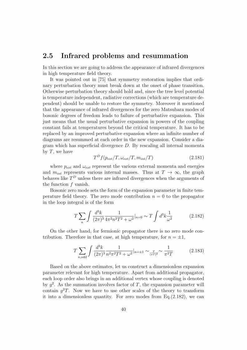
c . Now the one loop contribution to the self-energy of Fig. 2.3is quadratically divergent (D = 2), and so from Eq.(2.181), it will behave
Figure 2.3: One-loop contribution to the scalar self-energy.
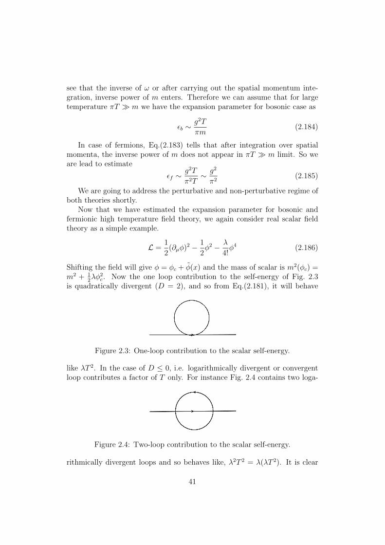
like λT 2. In the case of D ≤ 0, i.e. logarithmically divergent or convergentloop contributes a factor of T only. For instance Fig. 2.4 contains two loga-
Figure 2.4: Two-loop contribution to the scalar self-energy.
rithmically divergent loops and so behaves like, λ2T 2 = λ(λT 2). It is clear
41
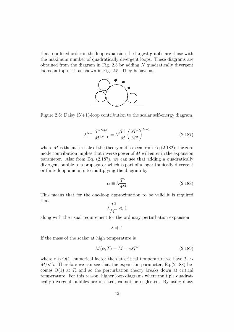
that to a fixed order in the loop expansion the largest graphs are those withthe maximum number of quadratically divergent loops. These diagrams areobtained from the diagram in Fig. 2.3 by adding N quadratically divergentloops on top of it, as shown in Fig. 2.5. They behave as,
Figure 2.5: Daisy (N+1)-loop contribution to the scalar self-energy diagram.
λN+1 T2N+1
M2N−1= λ2T
3
M
(λT 2
M2
)N−1
(2.187)
where M is the mass scale of the theory and as seen from Eq.(2.182), the zeromode contribution implies that inverse power of M will enter in the expansionparameter. Also from Eq. (2.187), we can see that adding a quadraticallydivergent bubble to a propagator which is part of a logarithmically divergentor finite loop amounts to multiplying the diagram by
α ≡ λT 2
M2(2.188)
This means that for the one-loop approximation to be valid it is requiredthat
λT 2
M2 1
along with the usual requirement for the ordinary perturbation expansion
λ 1
If the mass of the scalar at high temperature is
M(φ, T ) = M + cλT 2 (2.189)
where c is O(1) numerical factor then at critical temperature we have Tc ∼M/√λ. Therefore we can see that the expansion parameter, Eq.(2.188) be-
comes O(1) at Tc and so the perturbation theory breaks down at criticaltemperature. For this reason, higher loop diagrams where multiple quadrat-ically divergent bubbles are inserted, cannot be neglected. By using daisy
42
resummation technique [90, 91], one can consistently resum all powers of αand provides a theory where mass of the theory becomes m2(φc) → m2
eff ≡m2(φc) + Π(T ), where Π(T ) is the self-energy corresponding to the one-loopresummed diagram of order O(T 2).
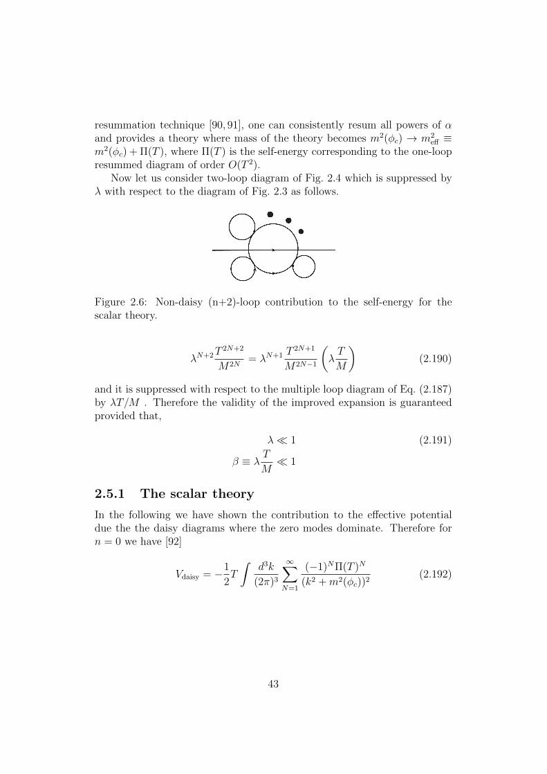
Now let us consider two-loop diagram of Fig. 2.4 which is suppressed byλ with respect to the diagram of Fig. 2.3 as follows.
Figure 2.6: Non-daisy (n+2)-loop contribution to the self-energy for thescalar theory.
λN+2T2N+2
M2N= λN+1 T
2N+1
M2N−1
(λT
M
)(2.190)
and it is suppressed with respect to the multiple loop diagram of Eq. (2.187)by λT/M . Therefore the validity of the improved expansion is guaranteedprovided that,
λ 1 (2.191)
β ≡ λT
M 1
2.5.1 The scalar theory
In the following we have shown the contribution to the effective potentialdue the the daisy diagrams where the zero modes dominate. Therefore forn = 0 we have [92]
Vdaisy = −1
2T
∫d3k
(2π)3
∞∑N=1
(−1)NΠ(T )N
(k2 +m2(φc))2(2.192)
43
where Π(T ) are the one loop bubble diagrams which are independent of theloop momentum k. Using Eq.(A.12) we have
Vdaisy = −1
2T∞∑N=1
1
N(−Π(T ))N
π32
Γ(32)(2π)3
(m2(φc))32−N Γ(3
2)Γ(N − 3
2)
Γ(N)
= − T
16π32
∞∑N=1
1
N(−1)N
(Π(T )
m2(φc)
)Nm3(φc)
Γ(N − 32)
Γ(N)
= −m3(φc)T
12π
∞∑N=1
(−1)N3
4√π
(Π(T )
m2(φc)
)N Γ(N − 32)
Γ(N + 1)
= − T
12π[(m2(φc) + Π(T ))
32 −m3(φc)] (2.193)
Therefore the effective potential is
Veff(φc) = V0(φc) + VCW(φc) + V(1)T (φc, T ) + Vdaisy(φc, T ) (2.194)
And taking the high temperature expansion of thermal effective potentialV
(1)T (φc, T ) and recollecting terms which are relevant for present case, we
have,
V (φc, T ) =1
2(m2 +
λ
12T 2)φ2
c −T
12π(m2(φc) + Π(T ))
32 +
λ
4φ4c + · · · (2.195)
In the limit, m2 + Π(T ) λφ2c , the potential (2.195) yields a first order
phase transition. At T ∼ Tc, we have the mimimum,
φc ∼√λTc (2.196)
Then from Eq.(2.191), with M ∼ m2(φc, T ) and considering the limit m2 +Π(T ) λφ2
c again we have,
β ∼ λTcλTc
= O(1) (2.197)
which indicates that the expansion parameter is of O(1) and therefore per-turbation theory is invalidated for first order phase transition shown by thescalar theory. On the other hand if m2 + Π(T ) is significantly larger, it willreduce the order parameter and the transition will cease to be first order.
2.5.2 The Standard Model
For the Standard Model, where there are gauge and Yukawa interactions, thecase is different from the previous example of the scalar theory. From thesimplified effective potential of the SM, Eq.(2.162) and Eq.(2.167) we have
44
φc ∼g3
λTc (2.198)
Here we have only considered the contribution of transverse gauge bosons tothe phase transition strength, and neglected that of the (screened) longitu-dinal gauge bosons.
The expansion parameter β associated with the Standard Model is,
βSM ∼ g2 T
mW (φ)(2.199)
Therefore at the vicinity of the symmetry breaking mimimum,
βSM ∼ gTcφc∼ λ
g2∼ m2
H
m2W
(2.200)
For this reason, in the Standard Model, the validity of the perturbation the-ory implies that mH mW and as this requirement is already invalidated bythe experimental results, we have to extend the SM to accommodate strongfirst order electroweak phase transition within the validity of the perturbationtheory.
45
Chapter 3
Electroweak Baryogenesis: theneed for strong phase transition
The observed baryon asymmetry of the universe still does not have any satis-factory explanation and it requires us to explore possible beyond the standardmodel scenarios. In this chapter we have presented a telegraphic review ofthe electroweak baryogenesis and the requirement of strong first order elec-troweak phase transition in this scenario. Section 3.1 has described the keyingredients for successful baryogenesis. In section 3.2, we have describedthe features of electroweak baryogenesis briefly. In section 3.3, we have con-structed the sphaleron solution for SU(2) scalar multiplets, described thebaryon number violating rate at above and below the critical temperatureand showed how the sphaleron decoupling condition leads to strong first or-der electroweak phase transition. More detailed account on Baryogenesis canbe found in [93–99].
The baryon asymmetry of the universe is evident from
• The null observation of abundance of the antimatter in the universe.Naturally it is only found in the cosmic ray. The antiproton in thecosmic ray is produced as secondaries in collisions (pp→ 3p+ p). Theratio of the number density of anti-proton to proton is bounded bynpnp∼ 3 × 10⁻⁴ [100–104]. Also, the flux ratio of antihelium to helium
in the cosmic ray has the upper bound of 1.1× 10⁻⁶ [105].
• The baryon to photon ratio is,
η =nB − nB
nγ(3.1)
where nB, nB and nγ are the number density of baryon, antibaryonand photon respectively. This parameter is essential for big bang nu-
46
cleosynthesis (BBN) because abundances of 3He, 4He, D, 6Li and 7Liare sensitive to the value of η. From one measured value of deuteriumabundance (D/H), η is given as [106]
η = 6.28± 0.35× 10⁻¹⁰ (3.2)
• The Cosmic Microwave Background (CMB) radiation facilitates an in-dependent measurement of the baryon asymmetry of the universe be-cause the observed Doppler peaks of the temperature anisotropy inCMB are sensitive to the value of η [107] and the accuracy is bet-ter than the BBN measurement [108]. With measured value ΩBh
2 =0.02207± 0.00033 (68% limit) by Planck collaboration [9], η is
η = 6.1± 0.1× 10⁻¹⁰ (3.3)
η = nB/nγ (as nB ∼ 0) is a good measurement of baryon asymmetry atlate time because nB and nγ stay constant but at the early time, when thetemperature of the universe was low enough to decouple baryon violatingprocesses but still high enough to keep various heavy particles in thermalequilibrium, η is not suitable because the annihilation or decay of thoseheavy particles afterwards, would create photons. So, it is convenient toconsider entropy instead of number density of photons for expressing baryonto photon ratio.
s =π4
45ζ(3)3.91 nγ = 7.04 nγ and
nB − nBnγ
=1
7.04η (3.4)
3.1 Sakharov’s conditions for baryogenesis
Although the universe was initially baryon symmetric (nB ' nB) one needsto explain the matter-antimatter asymmetry observed today in the universe.Either one has to put it as an initial condition or there are some dynam-ical mechanism which would lead to the observed asymmetry. It was firstsuggested by Sakharov [11] that it is possible to produce a small baryon asym-metry in the early universe dynamically. The three ingredients necessary forbaryogenesis are:
1. Baryon number nonconservation This condition is obvious sincewe want to start with a baryon symmetric universe (∆B = 0) and evolveit to a universe where ∆B 6= 0. Although still lacking positive results fromexperiments searching for B non-conservation, the baryon asymmetry of theuniverse is a unique observational evidence in favour of it.
47
2. C and CP violation If C and CP were conserved, the rate of reactionswith particles would be the same as the rate with antiparticles. If the initialstate of the universe was C and CP symmetric, no charge asymmetry coulddevelop from it. Consider the initial density matrix that commutes withC and CP operations, ρ0 = UC,CPρ0U
†C,CP and the Hamiltonian, H of the
system is C and CP invariant. If the time evolution operator is U(t) =exp(iHt), the density matrix at time t, ρ(t) = U(t)ρ0U(t)† will also be C andCP invariant. In such cases, the average of any C or CP odd operator, forexample B and L, is zero.
Here we elaborate more on the role of this second condition in baryonasymmetry. Consider a process A→ B+C that produces baryon B. Chargeconjugation of this process is A → B + C. So the net production rate ofbaryon is
dB
dt∼ Γ(A→ B + C)− Γ(A→ B + C) (3.5)
When charge conjugation is a symmetry, we have
Γ(A→ B + C) = Γ(A→ B + C) (3.6)
Therefore, Eq.(3.5) yields zero net production of baryon. But C violationalone is not enough for baryon asymmetry. One also requires CP violationin conjunction with C violation. Let us first denote the how left and righthanded fermions transform under P, C and CP:
P : ψL −→ ψR, ψR −→ ψL (3.7)
C : ψL −→ ψCL ≡ iσ2ψ∗R, ψR −→ ψCR ≡ −iσ2ψ
∗L
CP : ψL −→ ψCR , ψR −→ ψCL
Consider A decays into two left handed and two right handed quarks
A→ qL qL , A→ qR qR (3.8)
Now the C violation implies
Γ(A→ qL qL) 6= Γ(A→ qCL qCL )
Γ(A→ qR qR) 6= Γ(A→ qCR qCR) (3.9)
But CP invariance will imply that
Γ(A→ qL qL) = Γ(A→ qCR qCR)
Γ(A→ qR qR) = Γ(A→ qCL qCL ) (3.10)
48
When one adds up two decay channels,
Γ(A→ qL qL) + Γ(A→ qR qR) = Γ(A→ qCR qCR) + Γ(A→ qCL qCL ) (3.11)
For this reason, as long as we have equal number density for A and A, wewill not obtain any net quark asymmetry. The only asymmetry that will begenerated because of C violation is the asymmetry between number densityof left and right handed quarks.
3. Departure from thermal equilibrium As the consequence of CPTinvariance, if B violating process are in thermal equilibrium, the inverse pro-cess will wash out any the pre-existing asymmetry. For this reason a de-parture from thermal equilibrium is needed to retain the baryon asymmetryof the universe. There are several ways to achieve departure from equilibrium.
1. Out-of-equilibrium decay or scattering: In this case, the rate of inter-action must be smaller than the expansion rate of the universe, Γ < H.
2. Phase transition: First order phase transition proceeds through bubblenucleation which creates a temporary departure from equilibrium. Secondorder transition can’t provide such non-equilibrium condition as it doesn’thave any barrier between symmetric and broken phase and the transition iscontinuous.
3. Non-adiabatic motion of a scalar field: A coherent scalar field can betrapped in a local minimum of the potential but if the shape of the po-tential changes to become a maximum in such a way that the field maynot have enough time to re-adjust with the potential, it will onset a com-pletely non-adiabatic motion of the field. This is similar to a second orderphase transition but it is the non-adiabatic classical motion which prevailsover the quantum fluctuations, and therefore, departure from equilibriumcan be achieved. If such field condensate carries a global charge such as thebaryon number, the motion can charge up the condensate. Such mechanismhas been used in the Affleck-Dine baryogenesis [109] and its variants (forreview, [110,111]).
3.2 Electroweak baryogenesis
Electroweak Baryogenesis involves a first order phase transition which pro-ceeds through the nucleation of bubbles of broken phase within the surround-ing electroweak plasma in the symmetric phase. These bubbles expand, col-
49
lide and coalesce until the broken phase remains. Steps involving electroweakbaryogenesis are [99]:
• Particles in the electroweak plasma scatter at the bubble wall. If thetheory contains CP violation, this scattering can generate C and CPasymmetries in particle number densities in front of bubble wall.
• These asymmetries diffuse into symmetric phase ahead of bubble wall,where they will bias electroweak sphaleron transition to produce morebaryons than antibaryons.
• Some of the net baryon charge created outside the bubble wall is sweptup by the expanding wall into the broken phase. In the broken phase,the rate of sphaleron transition is strongly suppressed and can be smallenough to avoid washing away the baryons created in first two steps.
From the above steps of EWBG, we can see that Sakharov’s three con-ditions are satisfied manifestly. First, departure from thermal equilibrium isachieved by the rapidly expanding bubble walls through electroweak plasma.Second, violation of baryon number is provided by the rapid sphaleron transi-tion in the symmetric phase. And third, both C and CP violating scatteringprocesses of the particles at phase boundary create particle number asym-metries over those of antiparticles and this excess biases sphaleron transitionto create more baryons over antibaryons.
Anomalous nonconservation of fermion quantum numbers
Consider a theory with left handed ψL and right handed ψR fermions belong-ing to different representations of the gauge group. The partition function isgiven as
Z =
∫DAµDψDψeiS (3.12)
The following transformations
ψ′L = ei(QV −QA)α(x)ψL (3.13)
ψ′R = ei(QV +QA)α(x)ψR (3.14)
will induce additional terms in the action given by,
δS =
∫d4xψL(R)γ
µ(QV ∓QA)ψL(R)∂µα(x) (3.15)
50
The transformations also give rise to non-trivial Jacobian due to the non-invariance of the measure DψDψ. This anomaly can be expressed as theadditional contribution to the action as [112,113],
δSanomaly =
∫d4xα(x)[g2
L
QV −QA
16π2TrF (L)µνF(L)µν−g2
R
QV +QA
16π2TrF (R)µνF(R)µν ]
(3.16)where F (L)µν and F (R)µν are the field strengths with coupling constants gLand gR and they are coupled to left handed and right handed fermionic cur-rent respectively. Here, Fµν = 1
2εµνρσF
ρσ. First consider the transformationrelated to baryon number which is QV = 1
3and QA = 0. Now integrating by
parts Eq.(3.15) and requiring that the partition function is invariant underbaryonic number transformation, we have the baryon current in the standardmodel,
JµB =∑q
1
3qγµq (3.17)
to be anomalous,
∂µJµB =
NF
32π2(−g2F aµνF a
µν + g′2fµν fµν) (3.18)
where NF is the number of fermion generation, F aµν is the field strength of
SU(2)L and fµν is that of U(1)Y with coupling constants g and g′ respectively.Also here Tr(T aT b) = 1
2δab is used for SU(2)L generators and in the case of
U(1)Y , we have used Y = 1/6, 2/3,−1/3 for QL = (uL, dL), uR and dRrespectively.
Similarly for lepton number transformation we have QV = 1 and QA = 0.Therefore, following the same steps for Eq.(3.18), we have the lepton current,
JµL =∑l
(lγµl + νlγµνl) (3.19)
with it’s non vanishing divergence,
∂µJµL =
NF
32π2(−g2F aµνF a
µν + g′2fµν fµν) (3.20)
where Y = −1/2,−1 are used for lL = (νL, eL) and eR respectively in thecase of U(1)Y . Therefore we have
∂µJµB = ∂µJ
µL (3.21)
which shows that the current associated with B−L is conserved. Moreover,since each quark and lepton family gives same contribution to the anomaly
51
and as lepton flavor is conserved in the SM (because of neutrino mass beingzero in the SM at the renormlizable level), there are three conserved chargesin the SM
li =1
3B − Li (3.22)
where Li (i = e, µ, τ) are the leptonic flavors and∑
i Li = L.
Baryon number violation
The RHS of Eq.(3.18) can be re-expressed in the following way,
∂µJµB =
NF
32π2(−g2∂µK
µ + g′2∂µkµ) (3.23)
where
Kµ = εµνρσ(∂νWaρW
aσ −
1
3gεabcW
aνW
bρW
cσ) (3.24)
kµ = εµνρσ(∂νBρBσ) (3.25)
Here, W aµ and Bµ are the SU(2) and U(1) gauge field respectively.
The variation of the baryon number B =∫d3xJ0
B over time interval ∆tis ∆B. It is proportional to the variation of the Chern-Simons number overthe same time interval. The Chern-Simons numbers are defined as follows,
NCS = − g2
16π2
∫d3xεijkTr[∂iWjWk +
2i
3gWiWjWk] (3.26)
nCS = − g′2
16π2
∫d3xεijk∂iBjBk (3.27)
where NCS and nCS are associated with SU(2) and U(1) respectively. Thevariation of Chern-Simons number is related to the nonzero winding numberassociated with non-abelian gauge transformation.
Consider an element of SU(2), U = exp(iαaτa) which can also be writtenas U(x) = x0 + ixaτa where (x0, xa) ∈ R4. Because of UU † = U †U = 1, x0
and xa satisfies, x02 + xaxa = 1 which describes S3. As SU(2) is isomorphicto S3, U(x) can be associated with the mapping S3 → S3. The mappings~x→ U1(~x) and ~x→ U2(~x) will belong to the same equivalence class if thereexists a continuous deformation from U1(~x) to U2(~x). The equivalence class ischaracterized by positive or negative integer which is called winding number.This topological winding number n associated with U(x0, ~x) is
n = − 1
24π2
∫d3xεijkTr (AiAjAk) (3.28)
52
with Ai = ∂iU(x0, ~x)U−1(x0, ~x).Now first consider the transformation of SU(2), U (0) = 1 and it’s contin-
uous deformationU(x) = (1 + iεa(x)τa)U (0) (3.29)
For U (0) and any U(x), the winding number n[U ] is zero. On the other hand,for transformation
U (1) =x0 + i~x.~τ
r, r =
√x2
0 + |~x|2 (3.30)
we have n[U (1)] = 1. This result also holds for any continuous deforma-tion of U (1). Furthermore, if U (n) = [U (1)]n, we have n[U (n)] = n. So theSU(2) gauge transformation is divided into two classes: those which havezero winding numbers and those which have non-zero winding numbers.
Now under the U(1) gauge transformation Bi → Bi + ig′∂iUU
−1 where
U = eiα(x), nCS remains unchanged. On the other hand, SU(2) gauge trans-formation for which one has non-zero winding number Eq.(3.28), will inducenon-vanishing variation of NCS,
δNCS = − 1
24π2
∫d3x εijkTr(U∂iU
−1 · U∂jU−1 · U∂kU−1). (3.31)
Classically the ground state of the gauge theory should be time inde-pendent field configuration with vanishing energy density. Therefore wehave F a
µν = 0 which implies that the gound state will be pure gauge state~Wvac = i
g∇UU−1. Furthermore, the transformation U is required to satisfy
U → 1 as |~x| → ∞. For SU(2)L gauge theory with Higgs field Φ, in thetemporal gauge, W0 = 0, we have the vacuum defined as
W(0)i =
i
g∂iU
(0)U (0)−1
Φ(0) = (0, v/√
2)
NCS = 0
Using the gauge transformation U (n), we can have classically degeneratevacua with different Chern-Simons numbers as follows
W(n)i =
i
g∂iU
(n)U (n)−1
Φ(n) = U (n)Φ(0)
NCS = n
53
As ∆B is proportional to the change of the Chern-Simons number, nCSassociated with U(1), will not contribute to ∆B. So, when the system makesa transition from n-th vacuum to n+1-th vacuum, the Chern-Simons numberchanges by one unit and therefore the variations in B, L and B + L are,
∆B = ∆L = Nf ,∆(B + L) = 2Nf (3.32)
For the SM, number of generation is Nf = 3. When ∆NCS = 1, the vacuumto vacuum transition, because of fermion number nonconservation, will leadto the production of 9 left handed quarks (3 color states for each generations)and 3 left handed leptons so that ∆B = ∆L = 3. Moreover, in the SM∆(B + L) = 6 whereas proton decay, p → e+π0 requires ∆(B + L) = 2.Therefore, despite having B violation due to the anomaly, proton decay isforbidden in the SM. The probability amplitude for tunneling from n-thvacuum to n+ ∆NCS was estimated by WKB method [114,115],
P (∆NCS) ∼ exp(−4π∆NCS
αW) ∼ 10−162∆NCS (3.33)
which implies that baryon number violation in the SM is completely negligibleat zero temperature.
3.3 Baryon number violation at finite tem-
perature by the sphaleron
As already pointed out in Section 3.2, in the Standard Model (SM), theanomalous baryonic and leptonic currents lead to fermion number non-conservationbecause of the instanton induced transitions between topologically distinctvacua of SU(2) gauge fields [114, 115] and at zero temperature, the rateis of the order, e−2π/αw , αw ∼ 1/30, which is irrelevant for any physicalphenomena. However, there exists static unstable solution of the field equa-tions, known as sphaleron [13, 14, 116, 117], that represents the top of theenergy barrier between two distinct vacua and at finite temperature, be-cause of thermal fluctuations of fields, fermion number violating vacuum tovacuums transition can occur which is only suppressed by a Boltzmann fac-tor which contains the height of the barrier at the given temperature, i.e.the energy of the sphaleron [12]. Such baryon number violation induced bythe sphaleron is one of the essential ingredients of Electroweak Baryogene-sis [15, 16, 19, 21, 118, 119] and therefore, it has been extensively studied notonly in the SM [120–124,126–131] and but also in extended SM variants such
54
as, SM with a singlet [59, 132], two higgs doublet model [133], Minimal Su-persymmetric Standard Model [134], the next-to-Minimal SupersymmetricStandard Model [135] and 5 dimensional model [136].
3.3.1 Sphaleron in SU(2)L scalar representation
The standard way to find sphaleron solution in the Yang-Mills-Higgs theoryis to construct the non-contractible loops in the field space [14]. As thesphaleron is a saddle point solution of the configuration space, it is reallyhard to find them by solving the full set of equations of motion. Instead onestarts from an ansatz depending on a parameter µ that characterizes the non-contractible loop in the configuration space and corresponds to the vacuumfor µ = 0 and π while µ = π
2corresponds the highest energy configuration, in
other words, the sphaleron. In the following, we have focused on determiningthe energy functional and profile functions for the sphaleron in the SM forgeneral scalar multiplet [137].
Consider the scalar multiplet Q, charged under SU(2)L × U(1)Y group,is in J representation and has U(1) charge Y . The generators in this rep-resentation are denoted as Ja such that, Tr[JaJ b] = D(R)δab where D(R)is the Dynkin index for the representation. We define the charge operator,Q = J3 + Y and require the neutral component (J3 = −Y ) of the multi-plet to have the vacuum expectation value. The gauge-scalar sector of theLagrangian is
L = −1
4F aµνF a
µν −1
4fµνfµν + (DµQ)†DµQ− V (Q), (3.34)
with scalar potential
V (Q) = −µ2Q†Q+ λ1(Q†Q)2 + λ2(Q†JaQ)2. (3.35)
It was shown in [59] that the kinetic term of the scalar field makes largercontribution to the sphaleron energy than the potential term. Therefore, forsimplicity, we have considered CP-invariant scalar potential involving singlescalar representation to determine the sphaleron solution. It is straight-forward to generalize the calculation for the potential with multiple scalarfields1.
1In fact, in the SM, one needs large couplings between Higgs and extra scalars to triggera strong first order phase transition.
55
Also for convenience we elaborate,
F aµν = ∂µW
aν − ∂νW a
µ + gεabcW bµW
cν ,
fµν = ∂µBν − ∂νBµ,
DµQ = ∂µQ− igW aµJ
aQ− ig′BµY Q, (3.36)
where, g and g′ are the SU(2) and U(1) gauge couplings. The mixing angleθW is tan θW = g′/g.
The energy functional and variational equations
In the following, we have addressed the energy functional and the variationalequations of the sphaleron. The classical finite energy configuration are con-sidered in a gauge where the time component of the gauge fields are set tozero. Therefore the classical energy functional over the configuration is
E(W ai , Bi, Q) =
∫d3x[
1
4F aijF
aij +
1
4fijfij + (DiQ)†(DiQ) + V (Q)]. (3.37)
The non-contractible loop (NCL) in the configuration space is defined as map,S1×S2 ∼ S3 into SU(2) ∼ S3 using the following matrix U∞ ∈ SU(2) [126],
U∞(µ, θ, φ) = (cos2 µ+ sin2 µ cos θ)I2 + i sin 2µ(1− cos θ)τ 3
+ 2i sinµ sin θ(sinφτ 1 + cosφτ 2), (3.38)
where µ is the parameter of the NCL and θ, φ are the coordinates of thesphere at infinity. Also, τa are the SU(2) generators in the fundamentalrepresentation. We also define the 1-form in the following,
iU∞−1dU∞ =∑a
Faτa, (3.39)
which gives
F1 = −[2 sin2 µ cos(µ− φ)− sin 2µ cos θ sin(µ− φ)]dθ
− [sin 2µ cos(µ− φ) sin θ + sin2 µ sin 2θ sin(µ− φ)]dφ,
F2 = −[2 sin2 µ sin(µ− φ) + sin 2µ cos θ cos(µ− φ)]dθ
+ [sin2 µ sin 2θ cos(µ− φ)− sin 2µ sin θ sin(µ− φ)]dφ,
F3 = − sin 2µ sin θdθ + 2 sin2 θ sin2 µdφ. (3.40)
As shown in [126] the NCL starts and ends at the vacuum and consistsof three phases such that in first phase µ ∈ [−π
2, 0] it excites the scalar
56
configuration, in the second phase µ ∈ [0, π] it builds up and destroys thegauge configuration and in the third phase µ ∈ [π, 3π
2] it destroys the scalar
configuration.The field configurations in the first and third phases, µ ∈ [−π
2, 0] and
µ ∈ [π, 3π2
] aregW a
i τadxi = g′Bidx
i = 0, (3.41)
and
Q =v(sin2 µ+ h(ξ) cos2 µ)√
2
(0 .. 1 .. 0
)T, (3.42)
with ξ = gΩr is radial dimensionless coordinate and Ω is the mass parameterused to scale r−1, which we choose in what follows as Ω = mW/g. In thesecond phase µ ∈ [0, π], the field configurations are
gW ai τ
adxi = (1− f(ξ))(F1τ1 + F2τ
2) + (1− f3(ξ))F3τ3,
g′Bidxi = (1− f0(ξ))F3, (3.43)
and
Q =vh(ξ)√
2
(0 .. 1 .. 0
)T. (3.44)
Here, f(ξ), f3(ξ), f0(ξ) and h(ξ) are the radial profile functions. FromEq.(3.43), one can see that, in the spherical coordinate system, for the chosenansatz, the gauge fixing has led to, W a
r = Br = Bθ = 0. Moreover, similarto Eq.(3.43), the gauge fields acting on the scalar field Q can be written as
gW ai J
adxi = (1− f)(F1J1 + F2J
2) + (1− f3)F3J3. (3.45)
Finally the energy over the NCL for first and third phases is,
E(h, µ) =4πΩ
g
∫ ∞0
dξ[cos2 µv2
Ω2
1
2ξ2h′2 + ξ2V (h, µ)
g2Ω2], (3.46)
and for second phase,
E(µ, f, f3, f0, h, µ) =4πΩ
g
∫ ∞0
dξ[sin2 µ(8
3f ′
2+
4
3f ′3
2) +
8
ξ2sin4 µ2
3f 2
3 (1− f)2
+1
3f(2− f)− f32+
4
3(g
g′)2sin2 µf ′0
2+
2
ξ2sin4 µ(1− f0)2
+v2
Ω21
2ξ2h′
2+
4
3sin2 µh2(J(J + 1)− J2
3 )(1− f)2 + J23 (f0 − f3)2
+ξ2
g2Ω4V (h)]. (3.47)
57
From Eq.(3.47), the maximal energy is attained at µ = π2
which correspondsto the sphaleron configuration.
If there are multiple representations J (i) with non-zero neutral compo-nents J
(i)3 ,
Q(i) = vihi(ξ)√2
(0, .., 1.., 0)T , we have the energy of the sphaleron can be param-eterized as
Esph = E(µ =π
2) =
4πΩ
g
∫ ∞0
dξ[8
3f ′
2+
4
3f ′3
2+
8
3ξ22f 2
3 (1− f)2
+ (f(2− f)− f3)2+4
3(g
g′)2f ′0
2+
2
ξ2(1− f0)2+
∑i
1
2
v2i
Ω2ξ2h′i
2
+4
3h2i [2αi(1− f)2 + βi(f0 − f3)2]+ ξ2V (vihi)
g2Ω4], (3.48)
where the parameters
αi =(J (i)(J (i) + 1)− J (i)2
3 )v2i
2Ω2, βi =
J(i)23 v2
i
Ω2, (3.49)
refer to the scalar field couplings to the charged and neutral gauge fields.respectively.
The energy functional, Eq.(3.48) will be minimized by the solutions ofthe following variational equations
f ′′ +2
ξ2(1− f)[f(f − 2) + f3(1 + f3)] +
∑i
αih2i (1− f) = 0,
f ′′3 −2
ξ2[3f3 + f(f − 2)(1 + 2f3)] +
∑i
βih2i (f0 − f3) = 0,
f ′′0 +2
ξ2(1− f0)− g′2
g2
∑i
βih2i (f0 − f3) = 0,
h′′i +2
ξh′i −
8Ω2
3v2i ξ
2hi[2αi(1− f)2 + βi(f0 − f3)2]− 1
g2viΩ2
∂
∂φiV (φ)
∣∣∣∣φk=vkhk
= 0,
(3.50)
with the boundary conditions for (3.50) are given by: f(0) = f3(0) = h(0) =0, f0(0) = 1 and f(∞) = f3(∞) = f0(∞) = hi(∞) = 1. For g′ → 0, wehave, f0(ξ) → 1. The behavior of the field profiles Eq.(3.50) at the limitsξ → 0 and ξ → ∞ are given in appendix D. According to the last term inboth first and second lines in Eq.(3.50), it seems that the couplings of thescalar to gauge components, i.e (3.49), will play the most important role onthe shape of the field profiles as well the sphaleron energy.
58
Estimating the energy of the sphaleron
The sphaleron is therefore the solution which interpolates between the vac-uum at NCS = 0 (for ξ → 0) and the vacuum with NCS = 1 (for ξ →∞). Theenergy and the typical dimension of the sphaleron configuration are basicallythe result of the competition between the energy of the gauge configurationand the energy of the Higgs field. The latter introduces the weak scale intothe problem.
For the doublet case, we can set (J, Y ) = (1/2, 1/2) in Eq.(3.48) andEq.(3.50) to determine the energy of the sphaleron and field profiles numer-ically. In fact, this investigation has been carried out in [137] for scalarmultiplets, (J, Y ) = (1/2, 1/2), (1, 0), (1, 1), (3/2, 1/2), (3/2, 3/2), (2, 0), (2, 1)and (2, 2). But as our main focus is on the Higgs doublet of the SM, theresults regarding larger representations are not presented here. The quanti-tative numerical results for Higgs doublet case is already presented in [14].Still qualitative estimate can give a more physical intuitive picture of thesphaleron. As we pointed out before, the potential energy of the Higgs fieldis less important so for the sphaleron configuration of dimension l, we have
Wi ∼1
gl,
E(Wi) ∼4π
g2l, (3.51)
while the energy of the Higgs field is
E(φ) ∼ 4πv2l. (3.52)
Minimizing the sum E(Wi) + E(φ), we obtain that the typical dimension ofthe sphaleron is
lsp ∼1
gv∼ 10−16 cm, (3.53)
and
Esp ∼8πv
g∼ 10 TeV. (3.54)
The energy of the sphaleron in the case for doublet can be recast into thefollowing form,
Esp =4πv
gB(
λ
g2) (3.55)
where B is a function which depends very weakly on λ/g2: B(0) ' 1.52 andB(∞) ' 2.72. Inclusion of the mixing angle θW changes the energy of thesphaleron at most of 0.2%. The calculation done so far for the sphaleron
59
energy is when the temperature is zero. However, it was shown that at finitetemperature, its energy follows approximately the scaling law
Esp(T ) = Espφ(T )
v, (3.56)
where φ(T ) is the VEV of the Higgs field at finite temperature in the brokenphase. This energy can be re-written as
Esp(T ) =2mW (T )
αWB
(λ
g2
), (3.57)
where mW (T ) = 12gφ(T ) is the mass of W boson at finite temperature.
Moreover, the Chern-Simons number of the sphaleron can be computedin a straightforward manner by using Eq.(3.43) into Eq.(3.26) for µ = π
2and
one can obtain
N spCS =
1
2. (3.58)
3.3.2 Baryon number violation at T > Tc and T < Tc
The rate at T > Tc: At temperatures above the electroweak phase tran-sition, the vacuum expectation value of the Higgs field is zero, φ(T ) = 0, theHiggs field decouples and the sphaleron configuration ceases to exist.
Let us estimate the rate Γsp on dimensional grounds. As we mentioned,at high temperature T the Higgs field decouples from the dynamics and itsuffices to consider a pure SU(2) gauge theory. Topological transitions takeplace through the creation of non-perturbative, nearly static, magnetic fieldconfigurations that generate a change in the Chern-Simons number, ∆NCS
with a corresponding baryon number generation, ∆B = Nf∆NCS.If the field configuration responsible for the transition has a typical scale
l, a change ∆NCS ' 1 requires
∆NCS ∼ g2 l3 ∂AiAi ∼ g2l3AilAi ∼ 1⇒ Ai ∼
1
gl(3.59)
This means that the typical energy of the configuration is
Esp ∼ l3 (∂Ai)2 ∼ 1
g2l. (3.60)
To evade the Boltzmann suppression factor this energy should not be largerthan the temperature T , which requires
l >∼1
g2T. (3.61)
60
Such a length scale corresponds to the one of the dynamically generatedmagnetic mass of order g2T which behaves as a cut off for the maximumcoherence length of the system. The rate of one unsuppressed transition pervolume l3 and time t ∼ l is therefore
Γsp ∼1
l3t∼ (αW T )4. (3.62)
But it was pointed out in [138] that due to the damping effects in the plasma,the rate is suppressed by an extra power of αW to give Γsp ∼ α5
WT4. The
rate however is modified further as [139–141]
Γsym ∼ α5wT
4 ln(1/αw), (3.63)
From now on, we will parametrize the sphaleron rate in symmetric phase as
Γsp = κ(αW T )4. (3.64)
Therefore, it can be seen that in the symmetric phase, T > Tc, the baryonnumber violating processes are unsuppressed.
The Rate at T < Tc: Once the temperature drops off the critical one T <Tc, bubbles of true vacuum (φc 6= 0) start to nucleate where the sphaleronprocesses rate is suppressed as [124]
Γsp ∼ κ 2.8× 10⁵T 4(αW
4π
)4(
ξ(T )
B(λ/g2)
)7
e−ξ(T ) (3.65)
where, ξ(T ) = Esp(T )/T and B(λ/g2) is the function entering in Eq.(3.55).The factor κ is the functional determinant associated with fluctuations aroundthe sphaleron [16]. It has been estimated to be in the range: 10−4 . κ .10−1 [124,143].
B+L Washout
Considering the simplified case where all the conserved charges in the plasma(Q, Li, B − L, `i = B/3 − Li, · · · ) are zero. If we introduce a chemicalpotential for the charge B + L, µB+L, the free energy density of the system(fermions) is given by
F = T
∫d3k
(2π)3
[log
(1 + e−(Ek−µB+L)/T
)+ (µB+L → −µB+L)
]. (3.66)
61
The charge density of B + L may be expressed in terms of the chemicalpotential by
nB+L ∼ µB+LT2 (3.67)
and therefore we may relate the free energy with nB+L
F ∼ µ2B+LT
2 +O(T 4) ∼n2B+L
T 2+O(T 4). (3.68)
The free energy increases quadratically with the fermion number density andthe transitions which increase nB+L are energetically disfavored with respectto the ones that decrease the fermion number. If these transitions are activefor a long enough period of time, the system relaxes to the state of minimumenergy, i.e. nB+L = 0. Therefore any initial asymmetry in B + L relaxes tozero.
To address this issue more quantitatively, one has to consider the ratiobetween the transition rate with ∆NCS = +1, Γ+ and the one with ∆NCS =−1, Γ−,
Γ+
Γ−= e−∆F/T , (3.69)
where ∆F is the free energy difference between the two vacua that arises dueto the presence of chemical potential µB+L. If we define Γsp to be the averagebetween Γ+ and Γ−, we may compute the rate at which the baryon numberis being washed out [20]
dnB+L
dt= Γ+ − Γ− ' −
13
2NF
Γsp
T 3nB+L. (3.70)
Let us now consider temperatures much above the electroweak phase tran-sition, T mW . The exponential depletion of the nB+L due to the sphalerontransition remains active as long as
Γsp
T 3>∼ H ⇒ T <∼ α
4W
Mpl
g1/2∗∼ 1012 GeV. (3.71)
where the Hubble rate is H(T ) = 1.66√g∗T
2/Mpl. Therefore, at any tem-perature below T = 1012 GeV, the sphaleron transition will wash out anypre-existing B + L asymmetry with the time scale τ ∼ 2T 3/(13ΓspNF ).
3.3.3 Sphaleron decoupling and the strong EWPhTcondition
In the previous section, we can see that if the conserved charges in the plasmaare taken to be zero, the asymmetry generated in B, L or B + L will be
62
washed out by the sphaleron transitions if the system is kept in equilibriumfor sufficiently long period of time because these transitions do not conservethese charges. Therefore we require the B violating sphaleron transition toget out of equilibrium after the electroweak phase transition.
The dilution S = Bfinal/Binitial of the baryon asymmetry due to thesphaleron transition is
dS
dt=' −13
2NF
Γsp
T 3S (3.72)
Assuming T is constant during the phase transition the integration of Eq.(3.72)
yields S = e−X with X =13
2Nf
Γsp
T 3t. Using t = 3 × 10⁻²Mpl
T 2 and Eq.(3.65),
the exponent X is written as X ∼ 1010κξ7e−ξ, where we have taken the valuesof the parameters, B = 1.87, αW = 0.0336, Nf = 3, Tc ∼ 100 GeV. Now thefinal baryon asymmetry seen from the observation, is, Bfinal ∼ 10−8 − 10−10
and largest initial asymmetry in the SM can be Binitial ∼ 10−5−10−6 [20,142].Therefore, S >∼ 10−5 or we have X <∼ 10. This bound is translated into,
ξ(Tc) >∼ 7 log ξ(Tc) + 9 log 10 + log κ (3.73)
By considering first the upper bound of κ, κ = 10−1, we obtain fromEq.(3.73),
Esph(Tc)
Tc>∼ 45, (3.74)
and using the lower bound, κ = 10−4 we obtain,
Esph(Tc)
Tc>∼ 37, (3.75)
The bounds Eq.(3.74) and Eq.(3.75) put a condition on the ratio, φ(Tc)/Tc.From Eq.(3.57), at critical temperature Tc, we have
φ(Tc)
Tc=
g
4πB
Esph(Tc)
Tc∼ 1
36
Esph(Tc)
Tc(3.76)
where we have used the previous values of the parameters. The boundEq.(3.74) translates into
φ(Tc)
Tc>∼ 1.3 (3.77)
while the bound Eq.(3.75) translates into,
φ(Tc)
Tc>∼ 1.0 (3.78)
63
For a second order phase transition, φ(Tc) ' 0. So, the above bounds,Eq.(3.77) and (3.78), imply that the electroweak phase transition has tobe a strong first order transition so that the sphaleron transitions do notwash way the baryon asymmetry produced during the transition. However,it is already shown in section (2.4.2) that Higgs mass has to be below 45GeV to have strong electroweak phase transition (EWPhT). Furthermore,lattice studies [23–25] pointed out that for mh > 75 GeV, the transitionactually become a cross-over. Therefore, now with Higgs at 126 GeV, clearlyone can see the requirement of extending SM by new particles, possiblylying nearly the electroweak scale, which could provide strong EWPhT forsuccessful electroweak baryogenesis.
64
Chapter 4
Scalar representations in thelight of electroweak phasetransition and cold dark matterphenomenology
From chapter 2 and 3, we have seen that strong first order electroweak phasetransition required by the electroweak baryogenesis is not possible to obtainin the Standard Model because for this to happen, the Higgs mass has to bemuch smaller than the experimentally confirmed value. Also from chapter1, we have seen that, the observed dark matter of the universe lacks a sat-isfactory explanation with the SM. Therefore, we explore a class of modelswith extended scalar sector of the SM, generally known as the inert multipletmodel where we can achieve a strong first order phase transition and have adark matter candidate.
In this chapter we have focused on the correlation between the EWPhTand DM properties for various inert scalar representations and identified themost favorable candidate from this class of models [27,144]. In section 4.1, wehave presented the scalar potential and mass spectrum of the inert doublet,triplet and quartet model; an upper bound on the size of the multiplet andthe electroweak precision observables. In section 4.2 we have identified theregion of parameter space where strong EWPhT occurs for the inert doublet,complex tripet and quartet and also showed the impact of the size of themultiplet on the strength of the transition by calculating latent heat release.In section 4.3 we have presented the correlation between strong EWPhT anddark matter properties for the inert doublet case. Section 4.4 has featured therelic density analysis, direct detection limit for light DM in the quartet andfinally the correlation between the strong EWPhT and DM properties which
65
has indicated that the smaller representation is favorable than the larger onein providing a light DM and simultaneously trigger strong EWPhT.
4.1 Scalar representations beyond the Stan-
dard Model
4.1.1 Scalar multiplets with cold dark matter candi-dates
The scalar multiplet charged under SU(2)L × U(1)Y gauge group is char-acterized by (J, Y ). The electric charge for components of the multiplet isgiven by, Q = T3 + Y . For half integer representation J = n/2, T3 rangesfrom −n
2to n
2. So the hypercharge of the multiplet needs to be, Y = ±T3 for
one of the components to have neutral charge and can be considered as theDM. For integer representation n, similar condition holds for hypercharge.
When one considers the lightest component of the scalar multiplet as agood dark matter candidate [161], its lifetime has to be longer than about1026 sec which is set by the current experimental limits on the fluxes ofcosmic positrons, antiprotons and γ radiation [162, 163]. Such limits on thelifetime of the DM requires new couplings to be extremely small.1 Therefore,it is natural to adopt a Z2 symmetry under which all the SM particles areZ2 even and the extra scalars are Z2 odd such a way that the new couplingsdon’t arise in the Lagrangian which will lead to the decay of the dark matter.Also this Z2 symmetry becomes accidental for representations J ≥ 2 if weonly allow renormalizable terms in the Lagrangian. Moreover, our study isperformed in a region of parameter space where inert scalar multiplets donot develop any vev both in zero and finite temperature.2
Denoting scalar multiplet as Q, and the SM Higgs as Φ, the most generalHiggs-scalar multiplet potential , symmetric under Z2, can be written in thefollowing form,
V0(Φ, Q) = −µ2Φ†Φ +M2QQ†Q+ λ1(Φ†Φ)2 + λ2(Q†Q)2 + λ3|Q†T aQ|2
+ αΦ†ΦQ†Q+ βΦ†τaΦQ†T aQ+ γ[(ΦT ετaΦ)(QTCT aQ)† + h.c](4.1)
1For example, inert doublet can have yukawa coupling to fermions, yS ff , that can leadinto its decay. But for mDM ∼ 100 GeV (illustrating WIMP scale), the bound on DMlifetime, τDM ∼ 1025 − 1027 sec sets yS ∼ 10−25 − 10−27. Also five dimensional operator,εΛSF
µνFµν can induce DM decay into monochromatic gamma rays. But for mDM ∼ 100GeV and cut-off at EW scale, Λ ∼ v, the DM lifetime again sets ε ∼ 10−25 − 10−27.
2One can consider a scenario where inert multiplet can have non-zero vacuum expec-tation value at some finite temperature but it relaxes to zero as the temperature lowersdown. Such scenario has been explored for doublet [56] and real triplet [193].
66
Here, τa and T a are the SU(2) generators in fundamental and Q’s repre-sentation respectively. C is an antisymmetric matrix analogous to chargeconjugation matrix defined as,
CT aC−1 = −T aT (4.2)
C, being antisymmetric matrix, can only be defined for even dimensionalspace, i.e only for half integer representation. If the isospin of the reps.is j then C is a (2j + 1) × (2j + 1) dimensional matrix. The generatorsare normalized in such a way that they satisfy, for fundamental representa-tion, Tr[τaτ b] = 1
2δab and for other representations, Tr(T aT b) = D2(Q)δab.
Also T aT a = C2(Q). Here, D2(Q) and C2(Q) are Dynkin index and secondCasimir invariant for Q’s representation. The explicit form of generators, εand C matrix are given in section E.1. Notice that, γ term is only allowedfor representation with (J, Y ) = (n
2, 1
2).
For the doublet, real triplet, complex triplet, and the quartet, the scalarmultiplet Q is respectively
(C+
D0 ≡ 1√2(S + iA)
),
∆+
∆0
∆−
(Y=0)
,
∆++
∆+
∆0 ≡ 1√2(S + iA)
(Y=1)
, and
Q++
Q+
Q0 ≡ 1√2(S + iA)
Q′−
.
(4.3)In general, for the half-integer representation with (J, Y ) = (n
2, 1
2) and the
Integer representation with (J, Y ) = (n, Y = 0 or ±T3), the scalar multipletswith component fields denoted as ∆(Q), where Q is the electric charge, arerespectively
Qn2
=
∆(n+1
2)
...∆(0) ≡ 1√
2(S + i A)
...
∆(−n−12
)
and Qn =
∆(n)
...∆(0)
...∆(−n)
Y=0
. (4.4)
For the former representation every component represents a unique field whilefor the latter there is a redundancy ∆(−n) = (∆(n))∗ except the Y 6= 0 casefor which the component are also unique.
4.1.2 Inert Doublet, Triplet and Quartet mass spectra
Mass spectra: half integer representation with Y = 1/2 We nowsketch the general form of mass spectrum for the multiplet. As Y = 1/2, T3
67
value of the neutral component of the multiplet has to have T3 = −12. Now
for the Higgs vacuum expectation value, 〈Φ〉 = (0, v√2)T , the term 〈Φ†〉τ 3〈Φ〉
gives −v2
4. So masses for the neutral components, S and A are respectively
m2S = M2
Q+1
2(α+
1
4β+p(−1)p+1γ)v2 and m2
A = M2Q+
1
2(α+
1
4β−p(−1)p+1γ)v2.
(4.5)Here, p = 1
2Dim(n
2) = 1, 2, ... comes from 2p× 2p C matrix. For the charged
component, with T3 = j, we have,
m2(j) = M2
Q +1
2
(α− 1
2jβ
)v2. (4.6)
Now because of the γ term, there will be mixing between componentscarrying the same amount of charge. So to write down the mixing matrix,we have considered the ordering as follows. A component of the multipletis denoted as |J, T3〉. Components below the neutral component |n
2,−1
2〉 are
denoted with |n2,−1
2−m〉 where, m = 1, 2, ...., n−1
2and corresponding charge
is Q = −m. The piece 〈Φ〉T ετa〈Φ〉 gives v2
2√
2. Therefore, the mixing term
between between components with charge |Q| = m is,
(−1)m+1γv2
4
√(n+ 2m+ 1)(n− 2m+ 1)
In the ordering, (∆+( 1
2),∆+
(− 32
)), with m = 1, the mass matrix becomes,
M2+ =
m2( 1
2)
γv2
4
√(n+ 3)(n− 1)
γv2
4
√(n+ 3)(n− 1) m2
(− 32
)
(4.7)
And with m = 2 and (∆++( 3
2),∆++
(− 52
)) we have,
M2++ =
m2( 3
2)
−γv2
4
√(n+ 5)(n− 3)
−γv2
4
√(n+ 5)(n− 3) m2
(− 52
)
(4.8)
and so on, for charges with m = 3, 4, . . ..
68
Doublet model If we consider S of the inert doublet to be the DM can-didate, then following our parameterization Eq.(4.1) and Eq.(4.3), the massspectrum, is in the following
m2S = M2
Q +1
2
(α +
1
4β + γ
)v2
m2A = m2
S − γv2
m2C = m2
S −1
2
(γ +
1
2β
)v2 (4.9)
mS is the smallest mass in the spectrum when γ < 0 and γ + 12β < 0.
The couplings α, β and γ used in our parameterization is connected toλ3, λ4 and λ5 used in the literature, as follows,
λ3 = α− 1
4β , λ4 =
β
2, λ5 = γ (4.10)
Also, for convenience, we define,
λS = α +1
4β + γ , λA = α +
1
4β − γ , λC = α− 1
4β (4.11)
which are the couplings of S, A and C+ to the higgs.The conditions which ensure boundedness of the potential at large field
values for the doublet are
λ1 > 0 , λ2 > 0
α +1
4β > −2
√λ1λ2 in (h,C+, 0, ..) surface
α +1
4β + γ > −2
√λ1λ2 in (h, S, 0, ..) surface
Quartet model The immediate generalization of doublet case is the J =3/2 quartet case. Apart from splitting between S and A, γ term also mixestwo single charged components of the quartet. According to Eq.(4.7), themass matrix for the single charged fields in (Q+, Q
′+) basis is
M2+ =
(M2
Q + 12
(α− 1
4β)v2
√3
2γv2
√3
2γv2 M2
Q + 12
(α + 3
4β)v2
)(4.12)
Diagonalizing the mass matrix, we have mass eigenstates for single chargedfields, Q+
1 = Q+ cos θ + Q′+ sin θ, Q+
2 = −Q+ sin θ + Q′+ cos θ with tan 2θ =
−2√
3γβ
.
69
Again we consider S to be the dark matter. So masses of the componentsof the multiplet are as follows,
m2S = M2
Q +1
2
(α +
1
4β − 2γ
)v2
m2A = m2
S + 2γv2
m2Q++ = m2
S −1
2(β − 2γ)v2
m2Q+
1 (Q+2 )
= m2S +
(γ ∓ 1
4
√β2 + 12γ2
)v2 (4.13)
Because of the mixing between two single charged states, the mass relationis
m2S +m2
A = m2Q+
1+m2
Q+2
(4.14)
The full stability analysis for the quartet potential is an involved task sofor time being, we can give a partial set of necessary stability conditions bytaking Higgs-scalar two dimensional complex surface (h, ξi, 0, 0, ...) in fieldspace.3.
λ1 > 0 , λ2, λ3 > 0
α +1
4β − 2γ > −2
√λ1(λ2 +
1
4λ3) in (h, S, 0, ..) surface
α +1
4β + 2γ > −2
√λ1(λ2 +
1
4λ3) in (h,A, 0, ..) surface
α− 3
4β > −2
√λ1(λ2 +
3
4λ3) in (h,Q++, 0, ..) surface
α− 1
4β > −2
√λ1(λ2 +
1
4λ3) in (h,Q+, 0, ..) surface
α +3
4β > −2
√λ1(λ2 +
9
4λ3) in (h,Q′−, 0, ..) surface (4.15)
The last two conditions, when expressed in terms of mass eigenstates Q+1 , Q
+2
becomes
α∓ 1
4β(1∓2 cos 2θ)±
√3γ sin 2θ > −
√λ1λ2 +
1
4λ1λ3(3∓ 4 cos 2θ + 2 cos 4θ)
(4.16)in (h,Q+
1,2) surface.
3For general treatment see [164]
70
Mass spectra: integer representation with Y = 0 and Y 6= 0 Forinteger representation, γ term is not allowed. Therefore, there will not beany mass splitting between real and imaginary part of the neutral component.Moreover, for Y = 0 or real representation, the term Q†T 3Q is zero. So treelevel mass spectrum is degenerate and is given by,
m2∆ = M2
Q +1
2αv2. (4.17)
On the other hand, if Y 6= 0, there will be mass splitting due to β term. Alsoone can choose Y as, from −n to n, to set one component to be neutral. IfT3 = j, the mass is given by,
m2(j) = M2
Q +1
2
(α− 1
2βj
)v2 (4.18)
Triplet model Two representatives from this class are the real triplet (T =1, Y = 0) and the complex triplet (T = 1, Y = 1). For real triplet, the term,ƠT 3
T∆ is zero, so the mass spectrum will be degenerate and given as,
m2∆+ = m2
∆0 = M2∆ +
1
2αv2. (4.19)
On the other hand, for the complex case the mass spectrum is,
m2S = m2
A = M2∆ +
1
2
(α +
1
2β
)v2 (4.20)
m2∆+ = M2
∆ +1
2αv2 (4.21)
m2∆++ = M2
∆ +1
2
(α− 1
2β
)v2 (4.22)
There is a relation between masses:
m2∆++ −m2
∆+ = m2∆+ −m2
∆0 = −1
4βv2 (4.23)
And the stability conditions are,
λ1 > 0 , λ2, λ3 > 0
2α + β > −2√λ1(λ2 + λ3) in (h,∆0, 0, ..) surface
α > −2√λ1λ2 in (h,∆+, 0, ..) surface (4.24)
2α− β > −2√λ1(λ2 + λ3) in (h,∆++, 0, ..) surface (4.25)
71
When we don’t consider the Z2 symmetry and allow the new yukawa cou-plings with the complex triplet in the lagrangian, it will enable the neutrinoto acquire mass through the Type-II seesaw mechanism [165]. But in thatcase, the triplet will not able to provide any no viable DM candidate.
Because of the absence of γ term as in half integer representation, thereis no mass splitting between S and A of the neutral component ∆0. Sand A have vector interaction with Z boson that produces spin-independentelastic cross section which is already 8 − 9 orders of magnitude above theCDMS direct detection bound [166] and for this reason, complex triplet orany larger integer multiplet with non zero hypercharge is not going to satisfydirect detection bound as one will require a non-zero splitting between S andA larger than the kinetic energy of DM in our galactic halo to make Z−S−Aprocess kinematically forbidden. Therefore, only neutral component of thereal triplet can be a plausible DM candidate. In fact, real triplet DM has beenalready studied in [69, 70, 167, 168]. In [69, 167] it was shown that observedrelic density can be accounted for the DM if the mass of the DM lies about 2.5TeV. Being degenerate, one can easily see that, such particle would decouplefrom electroweak plasma and had no significant effect on EWPhT. But thequestion of having a strong first order EWPhT in complex triplet is relevantfor cosmic evolution of the universe. Therefore we only focused on EWPhTin the complex triplet case in a later section.
4.1.3 Perturbativity and EW physics constraints onthe size of the multiplets
Perturbativity: Landau pole of the gauge coupling, g
What is the largest possible inert multiplet allowed to be added to the stan-dard model? One possible bound comes from the beta function of SU(2)gauge coupling in presence of large scalar multiplets because the addition ofsuch large multiplet not only halts the asymptotic freedom of non-Abeliangauge couplings but also lowers the scale of landau pole with its size.
Consider non-abelian gauge theory with gauge group G and coupling g.If there are NF different fermion fields in different representations RF
i andNS scalar fields in different representations RS
i , the 1-loop beta function is
β(g) = µdg
dµ= − g3
16π2
[11
3T (A)− 2η
3
NF∑i=1
T (RFi )− 1
3
NS∑i=1
T (RSi )
]= − g3
16π2β
(4.26)Here, η = 1 (2) for Weyl (Dirac) fermions and β is the group theoretic factor.
72
Again, the Dynkin index of representation R, T (R) is define as
Tr (T aRTbR) = T (R)δab (4.27)
T (R) is determined from the following formula,
T (R) =dimR
dimGC2(R) (4.28)
where the quadratic Casimir of representation R is
T aRTaR = C2(R)IdimR (4.29)
Now by integrating Eq.(4.26) from µ0, where g(µ0) = g0, to µ whereg(µ) = g, we have,
g2 =1
1 +βg2
0
8π2 ln µµ0
(4.30)
Now if the matter contribution becomes larger than the gauge contributionin the beta function, β < 0. So the asymptotic freedom of non-abelian gaugetheory is lost and the landau pole will occur as follows,
Λlandau = µ0exp
(8π2
|β|g20
)(4.31)
where we can see that, the presence of larger representation of fermion andscalar fields increase |β| and therefore, the scale of landau pole, Λlandau be-comes smaller.
The one-loop beta function of SU(2) gauge coupling for Standard Modelsolely augmented by a scalar multiplet of isospin J is
β(g) =g3
16π2
(−19
6+
1
9J(J + 1)(2J + 1)
)(4.32)
It can be seen that, β(g) remains negative only for J ≤ 32. For, J ≥ 2, it
becomes positive and hits the landau pole as shown in Fig.(4.1). For instanceadding a scalar multiplet with isospin J ≥ 5 will bring the Landau pole ofSU(2) gauge coupling at Λ ≤ 10 TeV and for J ≥ 10, its even smaller,Λ ≤ 180 GeV. Therefore, perturbativity of gauge coupling at the TeV scalesets a upper bound on the size of the multiplet to be J ≤ 5.
73
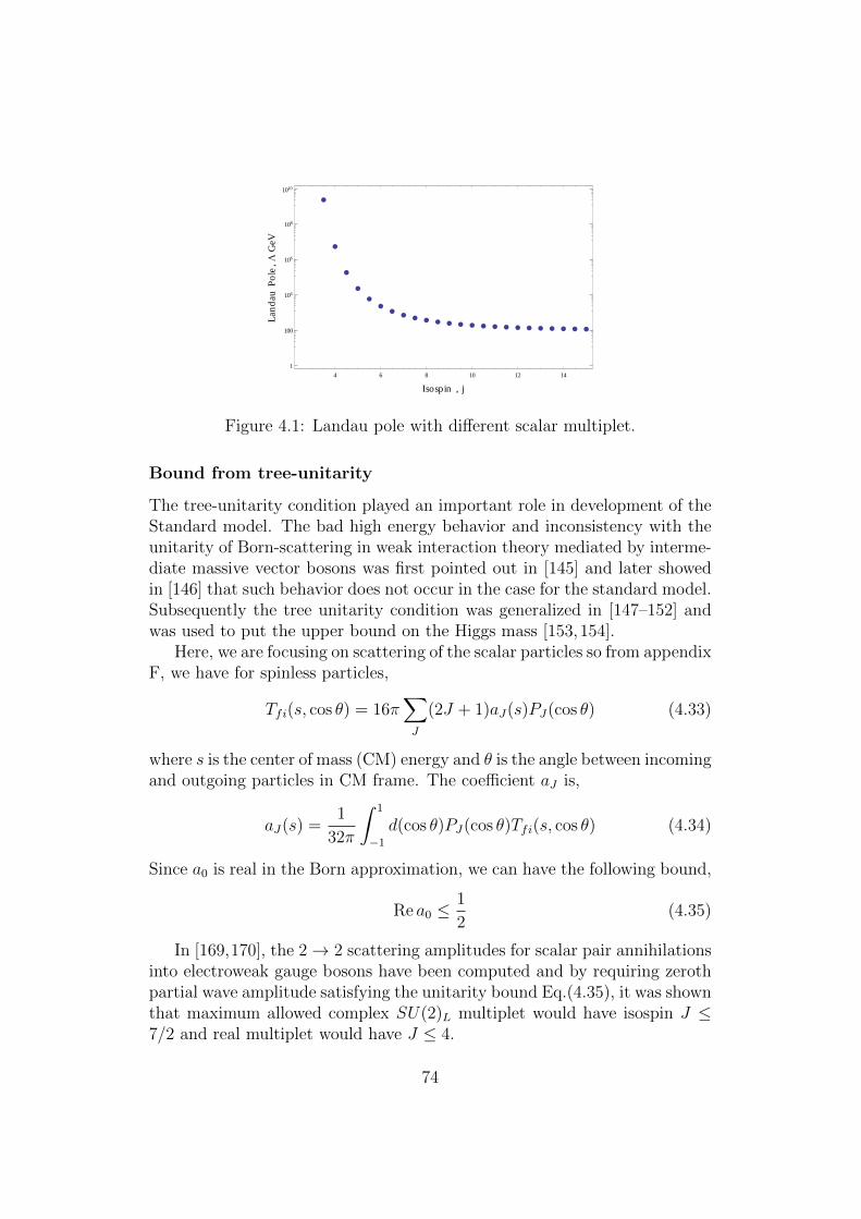
4 6 8 10 12 14
1
100
104
106
108
1010
Isospin , j
Lan
dau
Po
le,L
GeV
Figure 4.1: Landau pole with different scalar multiplet.
Bound from tree-unitarity
The tree-unitarity condition played an important role in development of theStandard model. The bad high energy behavior and inconsistency with theunitarity of Born-scattering in weak interaction theory mediated by interme-diate massive vector bosons was first pointed out in [145] and later showedin [146] that such behavior does not occur in the case for the standard model.Subsequently the tree unitarity condition was generalized in [147–152] andwas used to put the upper bound on the Higgs mass [153,154].
Here, we are focusing on scattering of the scalar particles so from appendixF, we have for spinless particles,
Tfi(s, cos θ) = 16π∑J
(2J + 1)aJ(s)PJ(cos θ) (4.33)
where s is the center of mass (CM) energy and θ is the angle between incomingand outgoing particles in CM frame. The coefficient aJ is,
aJ(s) =1
32π
∫ 1
−1
d(cos θ)PJ(cos θ)Tfi(s, cos θ) (4.34)
Since a0 is real in the Born approximation, we can have the following bound,
Re a0 ≤1
2(4.35)
In [169,170], the 2→ 2 scattering amplitudes for scalar pair annihilationsinto electroweak gauge bosons have been computed and by requiring zerothpartial wave amplitude satisfying the unitarity bound Eq.(4.35), it was shownthat maximum allowed complex SU(2)L multiplet would have isospin J ≤7/2 and real multiplet would have J ≤ 4.
74
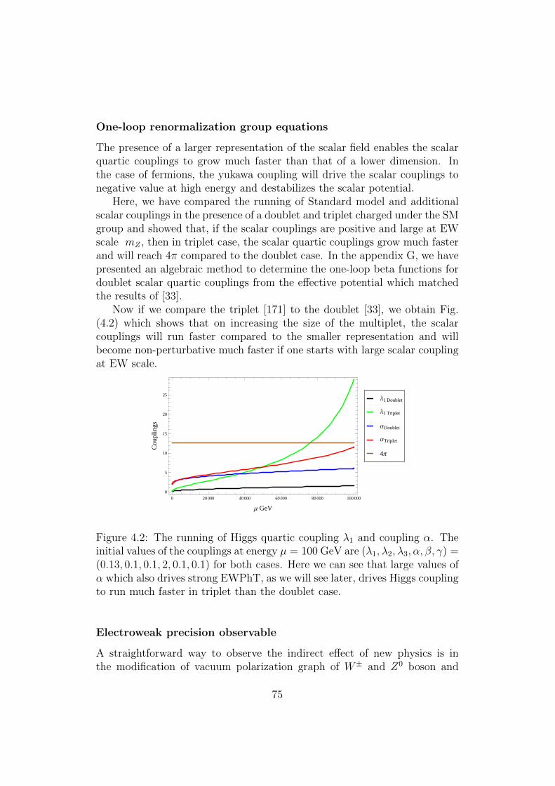
One-loop renormalization group equations
The presence of a larger representation of the scalar field enables the scalarquartic couplings to grow much faster than that of a lower dimension. Inthe case of fermions, the yukawa coupling will drive the scalar couplings tonegative value at high energy and destabilizes the scalar potential.
Here, we have compared the running of Standard model and additionalscalar couplings in the presence of a doublet and triplet charged under the SMgroup and showed that, if the scalar couplings are positive and large at EWscale mZ , then in triplet case, the scalar quartic couplings grow much fasterand will reach 4π compared to the doublet case. In the appendix G, we havepresented an algebraic method to determine the one-loop beta functions fordoublet scalar quartic couplings from the effective potential which matchedthe results of [33].
Now if we compare the triplet [171] to the doublet [33], we obtain Fig.(4.2) which shows that on increasing the size of the multiplet, the scalarcouplings will run faster compared to the smaller representation and willbecome non-perturbative much faster if one starts with large scalar couplingat EW scale.
0 20 000 40 000 60 000 80 000 100 000
0
5
10
15
20
25
Μ GeV
Cou
plin
gs
4Π
ΑTriplet
ΑDoublet
Λ1 Triplet
Λ1 Doublet
Figure 4.2: The running of Higgs quartic coupling λ1 and coupling α. Theinitial values of the couplings at energy µ = 100 GeV are (λ1, λ2, λ3, α, β, γ) =(0.13, 0.1, 0.1, 2, 0.1, 0.1) for both cases. Here we can see that large values ofα which also drives strong EWPhT, as we will see later, drives Higgs couplingto run much faster in triplet than the doublet case.
Electroweak precision observable
A straightforward way to observe the indirect effect of new physics is inthe modification of vacuum polarization graph of W± and Z0 boson and
75
one convenient way to parameterize these ’Oblique correction’ is through S,T and U parameters [172, 173] (analysis of one-loop correction in SM wasfirst done in [174]); plus V, W and X parameters [175] if new physics is atscale comparable to the EW scale. Oblique corrections are dominant overother ’non-oblique’ corrections (vertex diagram and box diagram with SMfermions as external states) because all the particles charged under SM groupwill couple to gauge bosons but usually only one or two particles in a theorywill couple to specific fermion species.
Because of the absence of coupling between inert scalar fields and SMfermions, the only dominant effects will come from oblique corrections. Tparameter, measuring the shift of ρ = MW
MZ cos θwfrom SM value due to the
radiative correction by new particles, is
αT =ΠWW (0)
m2W
− ΠZZ(0)
m2Z
(4.36)
where, ΠWW (0) and ΠZZ(0) vacuum polarization graph of W and Z bosonsevaluated at external momentum, p2 = 0.
EWPO in the Inert Doublet The contribution of the inert doublet toT parameter is [33]
T ≈ 1
24π2αv2(mC −mA)(mC −mS) . (4.37)
If the mass of the Higgs were heavier than the present value, one wouldthen require substantial T or a non-degenerate spectrum of the inert doubletstates. On the other hand, we are motivated by the first-order phase transi-tion, which favors as light SM Higgs, which is also confirmed experimentally.This in turn implies T ≈ 0. There are two possibilities to achieve this: a)mS < mC ≈ mA or b) mS ≈ mC < mA. It will turn out that S, as the DM,has to be lighter than about 80 GeV. It is not completely clear whether thepossibility b) is in accord with the experiment [176]. For this reason, we pur-sued possibility a), where A and C are quite degenerate [44] or equivalentlyγ ≈ β/2 (λ4 ≈ λ5).
As the scalar contribution to the S parameter is small compared to Tparameter, we have from [33],
S =1
2π
∫ 1
0
dxx(1− x)lnxm2
S + (1− x)m2A
m2C
(4.38)
76
EWPO for the Quartet The gauge-scalar-scalar vertices required forcalculating S and T parameters for the quartet are given in section E.2. Thequartet contribution to T parameter,
16π2α
g2T =
1
M2W
(3
2cos2 θ F (mQ++ ,mQ+
1) +
3
2sin2 θ F (mQ++ ,mQ+
2)
+1
4(√
3 sin θ + 2 cos θ)2 F (mQ+1,mS) +
1
4(√
3 sin θ − 2 cos θ)2 F (mQ+1,mA)
+1
4(√
3 cos θ − 2 sin θ)2 F (mQ+2,mS) +
1
4(√
3 cos θ + 2 sin θ)2 F (mQ+2,mA))
− 1
4c2wM
2Z
(F (mS,mA) + sin2 2θ F (mQ+1,mQ+
2)) (4.39)
here,
F (m1,m2) =m2
1 +m22
2− m2
1m22
m21 −m2
2
lnm2
1
m22
(4.40)
In addition, S parameter for quartet multiplet is,
S =s2w
8π
∫ 1
0
dx x(x− 1)[lnm2Q+
1
m2Q+
2
m4Q++
+ 2 cos 2θ lnm2Q+
2
m2Q+
1
+ ln(1− x)m2
S + xm2A
m2Q++
+ sin2 2θ ln[(1− x)m2
Q+1
+ xm2Q+
2
]2
m2Q+
1
m2Q+
2
] (4.41)
Best fit values of S and T The best fit values of S and T parameter with(U = 0)4 is [178]
S = 0.04± 0.09 and T = 0.07± 0.08 (4.42)
Therefore, one can put constraints on S and T parameter by comparing thetheoretical predictions with well measured experimental values of observ-ables.
4.2 Electroweak phase transition (EWPhT)
4.2.1 Finite temperature effective potential
In chapter 2, we have described the finite temperature effective potential indetails. Here we recapitulate the main points. If there are multiple classical
4The contribution to U parameter by scalar multiplet with only gauge interactionsconsidered in our case, will be smaller compared to T parameter by a factor (MW /MS)2,where MS is the leading scalar mass of theory [177]
77
background fields φi , which act as order parameters of the thermodynamicsystem, the total one-loop effective potential at finite temperature is,
Veff (φi, T ) = V0(φi) + VCW (φi) + VT (φi, T ) (4.43)
Here, V0, VCW and VT are tree-level, 1-loop Coleman-Weinberg and finitetemperature potential respectively. The daisy resummed finite temperaturepotential is,
VT =∑B(F )
(±)gB(F )T 4
2π2
∫ ∞0
dxx2 ln(1∓ e−√x2+m2
B(F )(φi,T )/T 2
) (4.44)
Here, gB and gF are bosonic and fermionic degrees of freedom and ± cor-respond to boson and fermion respectively. Thermal mass correction deter-mined with respect to background fields φj is,
m2i (φj)→ m2
i (φj, T ) = m2i (φj) + Πi(T ) (4.45)
where Πi(T ) is the thermal self energy correction (Debye correction) and atthe high temperature limit, it is of the form T 2 times coupling constants.Πi(T ) measures how much particles are screened by thermal plasma fromthe classical background field φ (just like the Debye screening) and largescreening reduces the strength of phase transition. In other words, it is theamplitude for the external particle (sourced by classical field) to forwardscatter off from a real physical particle present in the thermal bath [179].
For numerical convenience, in subsequent studies, we have used the fol-lowing form of the effective potential in high temperature approximation,
Veff = V0 + VCW +∑B
gB[m2B(φ, T )T 2
24− T
12π[m2
B(φ, T )]32 (4.46)
+m4B(φ, T )
64π2lnm2B(φ, T )
AbT 2] +∑F
gF
[m2F (φ)T 2
48− m2
F (φ)
64π2lnm2F (φ)
AfT 2
]It was shown in [17] that high T approximation agrees with exact potential
better than 5% for m/T < 1.6(2.2) for fermions (bosons). So unless greataccuracy is required, one can use Eq.(4.46) to explore the thermodynamicproperties of system.
Issue of imaginary effective potential and gauge dependence Therewill be some region of parameter space, for example, the Goldstone modes,where the effective potential will become imaginary due to the non-analytic
78
cubic terms (m2(φ, T ))32 and the log terms. It doesn’t signal the breakdown
of perturbative calculation, instead, as it was shown in [180, 184] that theimaginary part signals the instability of the homogeneous zero modes. More-over, as mentioned in [181] that the imaginary part vanishes when effectivepotential is calculated to all orders but at any finite order, it can be present.Therefore, in calculation we are only concerned with the real part of thepotential. To ameliorate the gauge dependence of finite temperature effec-tive potential, gauge invariant prescriptions have been developed [182–185].Moreover, in [184], it was shown that landau gauge (ξ = 0) is better in captur-ing the thermodynamic properties by comparing them with those determinedwith gauge invariant Hamiltonian formalism. So in this work we have chosento follow the landau gauge to carry out our numerical calculation. The mainmotivation for us is to explore the phase transition qualitatively and it’s al-ready apparent from the above discussion that perturbative techniques canat best capture the approximate nature of the finite temperature phenomena.For quantitative accuracy one eventually has to use lattice methods.
4.2.2 EWPhT with the Inert Doublet, Triplet and Quar-tet representations
The nature of electroweak phase transition is a cross over for Higgs boson withmass about 125.5 GeV (for a recent lattice study, [186]). Therefore to achievestrong first order phase transition, one must extend the scalar sector of thetheory. Consider an inert multiplet Q with isospin, j and hypercharge Y = 0and the parameter space is chosen in such a way that inert multiplet doesnot obtain any VEV at all temperatures. So, 〈Φ〉 = (0, φ√
2)T and 〈Q〉 = 0.
Because of zero VEV at all temperatures, the only classical background fieldis that of Higgs doublet and therefore the sphaleron configuration is exactlylike that of the Standard Model. For this reason, in this case, first orderphase transition is determined by the condition φc/Tc ≥ 1 as seen in section3.3.3.
The thermal masses for the component fields of the Higgs doublet Φ andreal multiplet Q are
m2h(φ, T ) = −µ2 + 3λ1φ
2 + a(j)T 2
12(4.47)
m2G±(φ, T ) = m2
G0(φ, T ) = −µ2 + λ1φ2 + a(j)
T 2
12
and due to degenerate mass spectrum,
m2i (φ, T ) = M2 +
1
2αφ2 + b(j)
T 2
12(4.48)
79
Temperature coefficients are,
a(j) = 6λ1 +1
2(2j + 1)α +
9
4g2 +
3
4g′2 + 3y2
t (4.49)
b(j) = (2j + 3)λ2 + 2α + 3j(j + 1)g2 (4.50)
Here one can see that from 1st and 3rd term of b(j) that larger representationreceives relatively large thermal corrections due to the scalar loops and gaugeboson loops. These coefficients capture how much particles are screenedby the plasma from the classical field which determines the strength of thetransition. The larger the coefficients are, the weaker the transition willbecome because those particles are effectively decoupled from the plasma.This plasma screening effect on the nature of phase transition for complexsinglet was already studied in [187]. In the following, we showed similareffect for real multiplet as it captures the essential features that depend onsize of the multiplet. Generalization to complex odd dimensional or evendimensional scalar multiplet is straightforward.
Using Eq.(4.46) and neglecting the terms coming from CW-correctionsand log terms we have,
VT (φ, T ) = A(T )φ2 +B(T )φ4 + C(T )[φ2 +K2(T )]32 (4.51)
where,
A(T ) = −1
2µ2 + a(j)
T 2
12(4.52)
B(T ) =1
4λ1
C(T ) = −(2j + 1)T
12π(α
2)
32
K2(T ) =2
α
(M2 + b(j)
T 2
12
)When the universe is at very high temperature, it is in the symmetric
vacuum φ = 0 but when the universe cools down, there can be two char-acteristic temperatures: T1 and T2. For temperature, T < T2, the origin isthe maximum and there is only one global minimum at φ 6= 0 that evolvestowards zero temperature minimum. For T > T2, the origin is a minimumand there is also a maximum at φ−(T ) and another minimum at φ+(T ) givenby,
φ2±(T ) =
1
32B2[9C2 − 16AB ± 3|C|
√9C2 + 32(2B2K2 − AB] (4.53)
80
The second order transition temperature T2 is determined by the condition,
4A2 − 9C2K2 = 0 (4.54)
And the first order transition temperature, T1 where VT (φc(T1), T1) = VT (0, T1)and φ+(T1) = φ−(T1) sets the condition,
9C2 + 32(2B2K2 − AB) = 0 (4.55)
From two conditions, T1 and T2 are determined as,
T 21 =
4λ1µ2 +
8M2+λ21
α
13a(j)λ1 − 2b(j)λ2
1
3α− (2j + 1)2 α3
128π2
(4.56)
and
T 22 =
1
2D(E +
√E2 − 4Dµ4) (4.57)
with
D =a(j)2
144− (2j + 1)2 b(j)α
2
768π2(4.58)
E =1
6a(j)µ2 + (2j + 1)2M
2α2
64π2
The nature of the transition depends on the relation between T1 andT2. If T1 > T2, the transition is first order and plasma screening is notso effective. When T1 < T2, the transition is actually second order due todominant plasma screening. Actually, T1 = T2 gives the turn over conditionfrom first to second order transition and from (4.56) and (4.57), we can havea condition on the parameter space (λ2, α,M, j).
3
256π2(2j + 1)2α4 − b(j)λ2
1 ≥ (a(j)λ1 −3
64π2(2j + 1)2α3)
(M
v
)2
(4.59)
Here, the strict inequality implies the region of parameter space where firstorder transition persists and equality corresponds to the turn-over. Here onecan see that, this inequality saturates if M and b(j) becomes large as thesetwo terms control the plasma screening for the particle. For small values ofα, we can easily see from LHS of (4.59) that the second term increases fasterthan the first term due to the quadratic Casimir for gauge boson contributionand self interacting quartic term in b(j) (Eq.(4.49)). Also if invariant massterm M is large, the RHS will saturates the inequality much faster. Soone can infer that although large representation will favor the first order
81
transition up to certain value of j because of more degrees of freedom in theplasma coupling to the background field, at one point, due to large thermalmass coming from gauge interaction, plasma screening will be large enoughto cease the first order transition and make it as a second order.
Electroweak phase transition with scalar singlet, two higgs doublet model5
[142,188–192] (and references therein) and real triplet [193] have been studiedextensively. Therefore, in the following sections, we have focused on theinert doublet, complex triplet and the quartet to study the nature of phasetransition.
Inert Doublet
The thermal mass for the Higgs and Goldstone fields are
m2h(φ, T ) = −µ2 + 3λ1φ
2 + aT 2
12(4.60)
m2G± = m2
G0 = −µ2 + λ1φ2 + a
T 2
12(4.61)
And thermal masses for the component fields of the inert doublet are
m2S(φ, T ) = M2
D +1
2(α +
1
4β + γ)φ2 + b
T 2
12(4.62)
m2A(φ, T ) = M2
D +1
2(α +
1
4β − γ)φ2 + b
T 2
12(4.63)
m2C(φ, T ) = M2
D +1
2(α− 1
4β)φ2 + b
T 2
12(4.64)
Here the thermal coefficients a and b are,
a = 6λ1 + 2α +9
4g2 +
3
4g′2 + 3y2
t (4.65)
b = 6λD + 2α +9
4g2 +
3
4g′2 (4.66)
MD and λD are denoting common mass term and self quartic coupling of theinert doublet respectively.
5Inert doublet can be considered as a special case of two Higgs doublet model
82
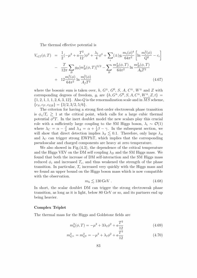
The thermal effective potential is
Veff (φ, T ) =1
2(−µ2 + a
T 2
12)φ2 +
λ1
4φ4 +
∑i
(±)gimi(φ)4
64π2
[lnm2i (φ)
Q2− ci
]− T
12π
∑B
gB[m2B(φ, T )]3/2 −
∑B
m4B(φ, T )
64π2lnm2B(φ, T )
AbT 2
+ 12m4t (φ)
64π2lnm2t (φ)
AfT 2(4.67)
where the bosonic sum is taken over, h, G±, G0, S, A, C±, W± and Z withcorresponding degrees of freedom, gi are h,G±, G0, S, A, C±,W±, Z, t =1, 2, 1, 1, 1, 2, 6, 3, 12. AlsoQ is the renormalization scale and inMS scheme,cS, cF , cGB = 3/2, 3/2, 5/6.
The criterion for having a strong first-order electroweak phase transitionis φc/Tc & 1 at the critical point, which calls for a large cubic thermalpotential φ3T . In the inert doublet model the new scalars play this crucialrole with a sufficiently large coupling to the SM Higgs boson, λi ∼ O(1)where λC = α − β
4and λA = α + 1
4β − γ. In the subsequent section, we
will show that direct detection implies λS . 0.1. Therefore, only large λAand λC can trigger strong EWPhT, which implies that the correspondingpseudoscalar and charged components are heavy at zero temperature.
We also showed in Fig.(4.3), the dependence of the critical temperatureand the Higgs VEV on the DM self coupling λD and the SM Higgs mass. Wefound that both the increase of DM self-interaction and the SM Higgs massreduced φc and increased Tc, and thus weakened the strength of the phasetransition. In particular, Tc increased very quickly with the Higgs mass andwe found an upper bound on the Higgs boson mass which is now compatiblewith the observation.
mh . 130 GeV . (4.68)
In short, the scalar doublet DM can trigger the strong electroweak phasetransition, as long as it is light, below 80 GeV or so, and its partners end upbeing heavier.
Complex Triplet
The thermal mass for the Higgs and Goldstone fields are
m2h(φ, T ) = −µ2 + 3λ1φ
2 + aT 2
12(4.69)
m2G± = m2
G0 = −µ2 + λ1φ2 + a
T 2
12(4.70)
83
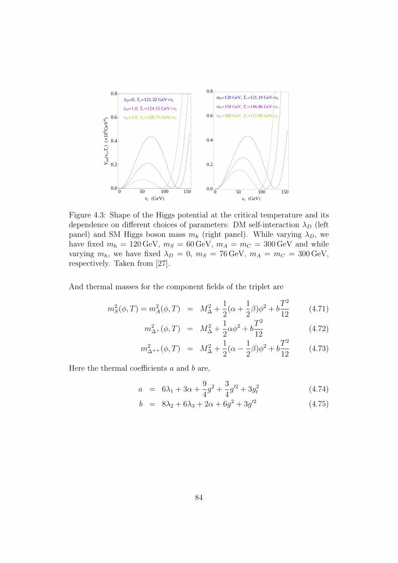
ΛD=0, Tc=121.32 GeV<vc
ΛD=1.0, Tc=124.15 GeV>vc
ΛD=3.0, Tc=128.75 GeV>vc
0 50 100 1500.0
0.2
0.4
0.6
0.8
vc HGeVL
Vto
tHvc,
TcL
H´10
6 GeV
4 Lmh=120 GeV, Tc=121.19 GeV<vc
mh=150 GeV, Tc=146.86 GeV>vc
mh=180 GeV, Tc=172.89 GeV>vc
0 50 100 1500.0
0.2
0.4
0.6
0.8
vc HGeVL
Figure 4.3: Shape of the Higgs potential at the critical temperature and itsdependence on different choices of parameters: DM self-interaction λD (leftpanel) and SM Higgs boson mass mh (right panel). While varying λD, wehave fixed mh = 120 GeV, mS = 60 GeV, mA = mC = 300 GeV and whilevarying mh, we have fixed λD = 0, mS = 76 GeV, mA = mC = 300 GeV,respectively. Taken from [27].
And thermal masses for the component fields of the triplet are
m2S(φ, T ) = m2
A(φ, T ) = M2∆ +
1
2(α +
1
2β)φ2 + b
T 2
12(4.71)
m2∆+(φ, T ) = M2
∆ +1
2αφ2 + b
T 2
12(4.72)
m2∆++(φ, T ) = M2
∆ +1
2(α− 1
2β)φ2 + b
T 2
12(4.73)
Here the thermal coefficients a and b are,
a = 6λ1 + 3α +9
4g2 +
3
4g′2 + 3y2
t (4.74)
b = 8λ2 + 6λ3 + 2α + 6g2 + 3g′2 (4.75)
84
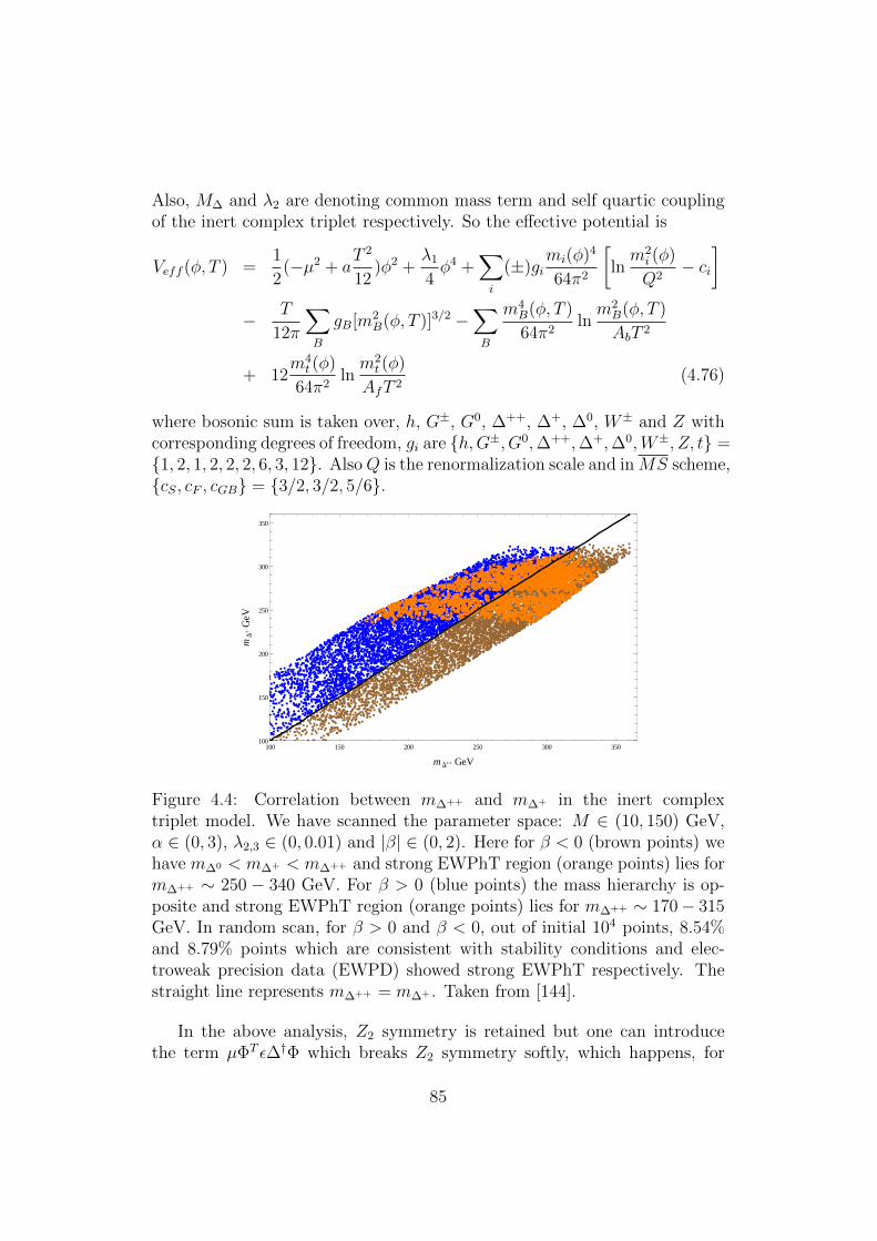
Also, M∆ and λ2 are denoting common mass term and self quartic couplingof the inert complex triplet respectively. So the effective potential is
Veff (φ, T ) =1
2(−µ2 + a
T 2
12)φ2 +
λ1
4φ4 +
∑i
(±)gimi(φ)4
64π2
[lnm2i (φ)
Q2− ci
]− T
12π
∑B
gB[m2B(φ, T )]3/2 −
∑B
m4B(φ, T )
64π2lnm2B(φ, T )
AbT 2
+ 12m4t (φ)
64π2lnm2t (φ)
AfT 2(4.76)
where bosonic sum is taken over, h, G±, G0, ∆++, ∆+, ∆0, W± and Z withcorresponding degrees of freedom, gi are h,G±, G0,∆++,∆+,∆0,W±, Z, t =1, 2, 1, 2, 2, 2, 6, 3, 12. AlsoQ is the renormalization scale and inMS scheme,cS, cF , cGB = 3/2, 3/2, 5/6.
100 150 200 250 300 350100
150
200
250
300
350
mD++ GeV
mD
+G
eV
Figure 4.4: Correlation between m∆++ and m∆+ in the inert complextriplet model. We have scanned the parameter space: M ∈ (10, 150) GeV,α ∈ (0, 3), λ2,3 ∈ (0, 0.01) and |β| ∈ (0, 2). Here for β < 0 (brown points) wehave m∆0 < m∆+ < m∆++ and strong EWPhT region (orange points) lies form∆++ ∼ 250 − 340 GeV. For β > 0 (blue points) the mass hierarchy is op-posite and strong EWPhT region (orange points) lies for m∆++ ∼ 170− 315GeV. In random scan, for β > 0 and β < 0, out of initial 104 points, 8.54%and 8.79% points which are consistent with stability conditions and elec-troweak precision data (EWPD) showed strong EWPhT respectively. Thestraight line represents m∆++ = m∆+ . Taken from [144].
In the above analysis, Z2 symmetry is retained but one can introducethe term µΦT ε∆†Φ which breaks Z2 symmetry softly, which happens, for
85
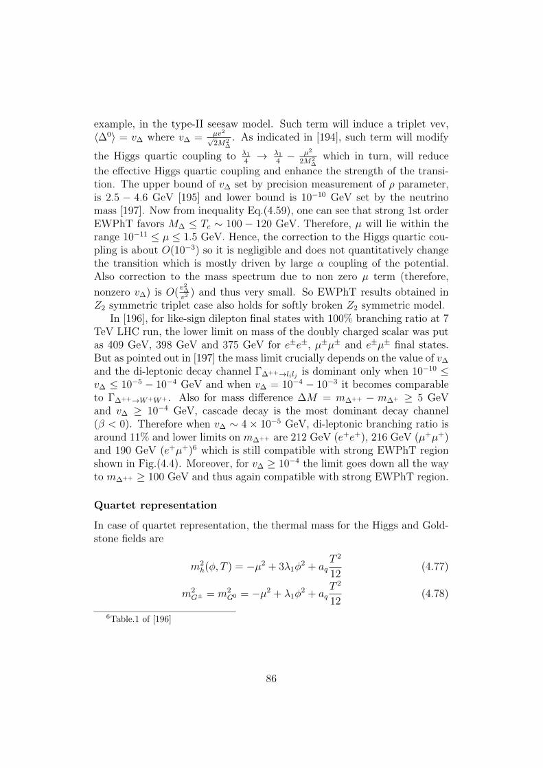
example, in the type-II seesaw model. Such term will induce a triplet vev,〈∆0〉 = v∆ where v∆ = µv2
√2M2
∆
. As indicated in [194], such term will modify
the Higgs quartic coupling to λ1
4→ λ1
4− µ2
2M2∆
which in turn, will reduce
the effective Higgs quartic coupling and enhance the strength of the transi-tion. The upper bound of v∆ set by precision measurement of ρ parameter,is 2.5 − 4.6 GeV [195] and lower bound is 10−10 GeV set by the neutrinomass [197]. Now from inequality Eq.(4.59), one can see that strong 1st orderEWPhT favors M∆ ≤ Tc ∼ 100 − 120 GeV. Therefore, µ will lie within therange 10−11 ≤ µ ≤ 1.5 GeV. Hence, the correction to the Higgs quartic cou-pling is about O(10−3) so it is negligible and does not quantitatively changethe transition which is mostly driven by large α coupling of the potential.Also correction to the mass spectrum due to non zero µ term (therefore,
nonzero v∆) is O(v2∆
v2 ) and thus very small. So EWPhT results obtained inZ2 symmetric triplet case also holds for softly broken Z2 symmetric model.
In [196], for like-sign dilepton final states with 100% branching ratio at 7TeV LHC run, the lower limit on mass of the doubly charged scalar was putas 409 GeV, 398 GeV and 375 GeV for e±e±, µ±µ± and e±µ± final states.But as pointed out in [197] the mass limit crucially depends on the value of v∆
and the di-leptonic decay channel Γ∆++→lilj is dominant only when 10−10 ≤v∆ ≤ 10−5 − 10−4 GeV and when v∆ = 10−4 − 10−3 it becomes comparableto Γ∆++→W+W+ . Also for mass difference ∆M = m∆++ − m∆+ ≥ 5 GeVand v∆ ≥ 10−4 GeV, cascade decay is the most dominant decay channel(β < 0). Therefore when v∆ ∼ 4 × 10⁻⁵ GeV, di-leptonic branching ratio isaround 11% and lower limits on m∆++ are 212 GeV (e+e+), 216 GeV (µ+µ+)and 190 GeV (e+µ+)6 which is still compatible with strong EWPhT regionshown in Fig.(4.4). Moreover, for v∆ ≥ 10−4 the limit goes down all the wayto m∆++ ≥ 100 GeV and thus again compatible with strong EWPhT region.
Quartet representation
In case of quartet representation, the thermal mass for the Higgs and Gold-stone fields are
m2h(φ, T ) = −µ2 + 3λ1φ
2 + aqT 2
12(4.77)
m2G± = m2
G0 = −µ2 + λ1φ2 + aq
T 2
12(4.78)
6Table.1 of [196]
86
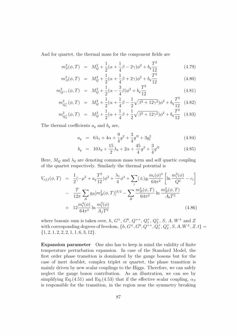
And for quartet, the thermal mass for the component fields are
m2S(φ, T ) = M2
Q +1
2(α +
1
4β − 2γ)φ2 + bq
T 2
12(4.79)
m2A(φ, T ) = M2
Q +1
2(α +
1
4β + 2γ)φ2 + bq
T 2
12(4.80)
m2Q++(φ, T ) = M2
Q +1
2(α− 3
4β)φ2 + bq
T 2
12(4.81)
m2Q+
1(φ, T ) = M2
Q +1
2(α +
1
4β − 1
2
√β2 + 12γ2)φ2 + bq
T 2
12(4.82)
m2Q+
2(φ, T ) = M2
Q +1
2(α +
1
4β +
1
2
√β2 + 12γ2)φ2 + bq
T 2
12(4.83)
The thermal coefficients aq and bq are,
aq = 6λ1 + 4α +9
4g2 +
3
4g′2 + 3y2
t (4.84)
bq = 10λ2 +15
2λ3 + 2α +
45
4g2 +
3
4g′2 (4.85)
Here, MQ and λ2 are denoting common mass term and self quartic couplingof the quartet respectively. Similarly the thermal potential is
Veff (φ, T ) =1
2(−µ2 + aq
T 2
12)φ2 +
λ1
4φ4 +
∑i
(±)gimi(φ)4
64π2
[lnm2i (φ)
Q2− ci
]− T
12π
∑B
gB[m2B(φ, T )]3/2 −
∑B
m4B(φ, T )
64π2lnm2B(φ, T )
AbT 2
+ 12m4t (φ)
64π2lnm2t (φ)
AfT 2(4.86)
where bosonic sum is taken over, h, G±, G0, Q++, Q+1 , Q+
2 , S, A, W± and Zwith corresponding degrees of freedom, h,G±, G0, Q++, Q+
1 , Q+2 , S, A,W
±, Z, t =1, 2, 1, 2, 2, 2, 1, 1, 6, 3, 12.
Expansion parameter One also has to keep in mind the validity of finitetemperature perturbation expansion. In case of the Standard Model, thefirst order phase transition is dominated by the gauge bosons but for thecase of inert doublet, complex triplet or quartet, the phase transition ismainly driven by new scalar couplings to the Higgs. Therefore, we can safelyneglect the gauge boson contribution. As an illustration, we can see bysimplifying Eq.(4.51) and Eq.(4.53) that if the effective scalar coupling, αSis responsible for the transition, in the region near the symmetry breaking
87
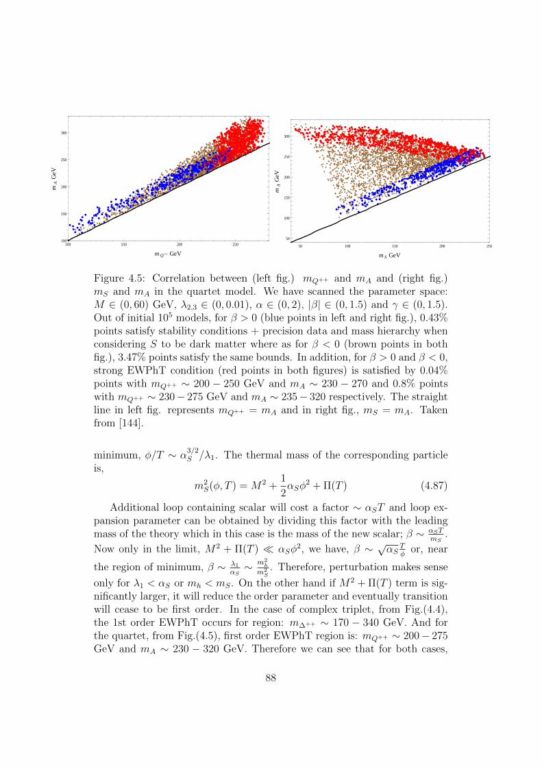
100 150 200 250100
150
200
250
300
mQ++ GeV
mA
GeV
50 100 150 200 250
50
100
150
200
250
300
mS GeV
mA
GeV
Figure 4.5: Correlation between (left fig.) mQ++ and mA and (right fig.)mS and mA in the quartet model. We have scanned the parameter space:M ∈ (0, 60) GeV, λ2,3 ∈ (0, 0.01), α ∈ (0, 2), |β| ∈ (0, 1.5) and γ ∈ (0, 1.5).Out of initial 105 models, for β > 0 (blue points in left and right fig.), 0.43%points satisfy stability conditions + precision data and mass hierarchy whenconsidering S to be dark matter where as for β < 0 (brown points in bothfig.), 3.47% points satisfy the same bounds. In addition, for β > 0 and β < 0,strong EWPhT condition (red points in both figures) is satisfied by 0.04%points with mQ++ ∼ 200 − 250 GeV and mA ∼ 230 − 270 and 0.8% pointswith mQ++ ∼ 230− 275 GeV and mA ∼ 235− 320 respectively. The straightline in left fig. represents mQ++ = mA and in right fig., mS = mA. Takenfrom [144].
minimum, φ/T ∼ α3/2S /λ1. The thermal mass of the corresponding particle
is,
m2S(φ, T ) = M2 +
1
2αSφ
2 + Π(T ) (4.87)
Additional loop containing scalar will cost a factor ∼ αST and loop ex-pansion parameter can be obtained by dividing this factor with the leadingmass of the theory which in this case is the mass of the new scalar; β ∼ αST
mS.
Now only in the limit, M2 + Π(T ) αSφ2, we have, β ∼ √αS Tφ or, near
the region of minimum, β ∼ λ1
αS∼ m2
h
m2S
. Therefore, perturbation makes sense
only for λ1 < αS or mh < mS. On the other hand if M2 + Π(T ) term is sig-nificantly larger, it will reduce the order parameter and eventually transitionwill cease to be first order. In the case of complex triplet, from Fig.(4.4),the 1st order EWPhT occurs for region: m∆++ ∼ 170 − 340 GeV. And forthe quartet, from Fig.(4.5), first order EWPhT region is: mQ++ ∼ 200− 275GeV and mA ∼ 230 − 320 GeV. Therefore we can see that for both cases,
88
the mass regions where first order transition occurs are larger than the Higgsmass and hence, within the validity of perturbation theory.
Other uncertainties? So far, we have worked in the improved one-loopapproximation for the effective potential at non-zero temperature, and so onecan question its reliability at higher orders in the perturbation theory. In fact,in the MSSM, it turns out that the two-loop effects [198] help to strengthenthe phase transition. Similarly, the non-perturbative lattice simulations tendto do the same over the perturbative results [199].
4.2.3 Impact of multiplets’ sizes on EWPhT
Latent heat release The phase transition is characterized by the releaseof latent heat. If there is a latent heat release, the transition is first order innature otherwise it is second or higher order (as in Ehrenfest’s classification).The nature of cosmological phase transition is addressed in [200,201]. In thissection, we have addressed how the size of the representation affects the latentheat release during the electroweak phase transition with assumption thatthe transition is first order driven by large Higgs-inert scalar coupling, i.e. α.Consider a system gone through first order phase transition at temperature,Tc. The high temperature phase consists of radiation energy and false vacuumenergy and energy density is denoted as ρ+. On the other hand, althoughlow temperature phase has equal free energy F it will have different energydensity, ρ−. The discontinuity ∆ρ(Tc) = ρ+(Tc) − ρ−(Tc), gives the latentheat, L = ∆ρ(Tc) = Tc∆s(Tc) where ∆s(Tc) = s+ − s− is entropy densitydifference and it is liberated when the region of high-T phase is convertedinto the low-T phase. Therefore, using F = ρ− Ts with s = −dF
dTand from
expression for effective potential (equivalent to free energy), Eq.(4.44) andas for 1st order phase transition, F+(0, Tc) = F−(φc, Tc), we have the latentheat for the transition,
L = TdF−dT|(φc,Tc) − T
dF+
dT|(0,Tc) (4.88)
For simplicity we can again take real degenerate representation for prob-ing the impact of dimension of large multiplet on the latent heat release. Asthe amount of latent heat represents the strength of first order transition, itis already clear from Fig.(4.6) that larger representation disfavors first orderphase transition. In addition, in section 4.1.3 we have seen that arbitrarilylarge scalar multiplet makes gauge and scalar couplings non-perturbative inTeV or even at smaller scale. Therefore, larger scalar multiplet cannot si-multaneously strengthen the electroweak phase transition and stay consistent
89
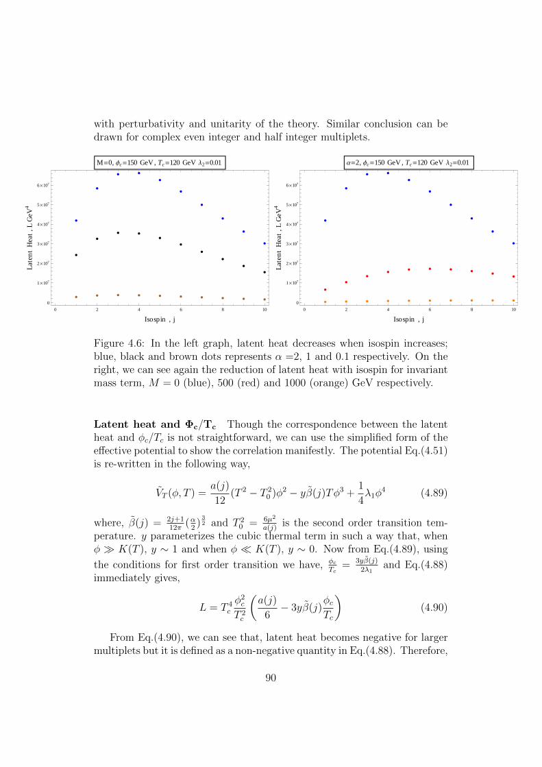
with perturbativity and unitarity of the theory. Similar conclusion can bedrawn for complex even integer and half integer multiplets.
0 2 4 6 8 10
0
1 ´ 107
2 ´ 107
3 ´ 107
4 ´ 107
5 ´ 107
6 ´ 107
Isospin , j
Lat
ent
Hea
t,L
GeV
4
M=0, Φc =150 GeV , Tc =120 GeV Λ2=0.01
0 2 4 6 8 10
0
1 ´ 107
2 ´ 107
3 ´ 107
4 ´ 107
5 ´ 107
6 ´ 107
Isospin , j
Lat
ent
Hea
t,L
GeV
4
Α=2, Φc =150 GeV , Tc =120 GeV Λ2=0.01
Figure 4.6: In the left graph, latent heat decreases when isospin increases;blue, black and brown dots represents α =2, 1 and 0.1 respectively. On theright, we can see again the reduction of latent heat with isospin for invariantmass term, M = 0 (blue), 500 (red) and 1000 (orange) GeV respectively.
Latent heat and Φc/Tc Though the correspondence between the latentheat and φc/Tc is not straightforward, we can use the simplified form of theeffective potential to show the correlation manifestly. The potential Eq.(4.51)is re-written in the following way,
VT (φ, T ) =a(j)
12(T 2 − T 2
0 )φ2 − yβ(j)Tφ3 +1
4λ1φ
4 (4.89)
where, β(j) = 2j+112π
(α2)
32 and T 2
0 = 6µ2
a(j)is the second order transition tem-
perature. y parameterizes the cubic thermal term in such a way that, whenφ K(T ), y ∼ 1 and when φ K(T ), y ∼ 0. Now from Eq.(4.89), using
the conditions for first order transition we have, φcTc
= 3yβ(j)2λ1
and Eq.(4.88)immediately gives,
L = T 4c
φ2c
T 2c
(a(j)
6− 3yβ(j)
φcTc
)(4.90)
From Eq.(4.90), we can see that, latent heat becomes negative for largermultiplets but it is defined as a non-negative quantity in Eq.(4.88). Therefore,
90
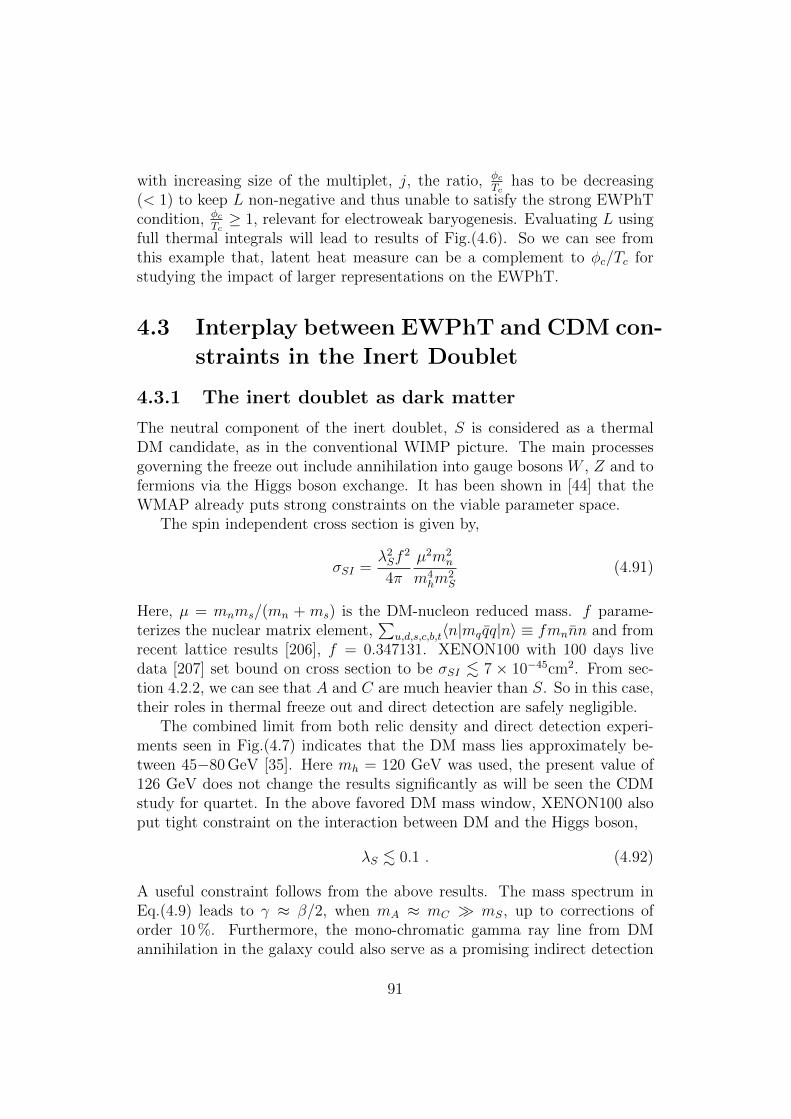
with increasing size of the multiplet, j, the ratio, φcTc
has to be decreasing(< 1) to keep L non-negative and thus unable to satisfy the strong EWPhTcondition, φc
Tc≥ 1, relevant for electroweak baryogenesis. Evaluating L using
full thermal integrals will lead to results of Fig.(4.6). So we can see fromthis example that, latent heat measure can be a complement to φc/Tc forstudying the impact of larger representations on the EWPhT.
4.3 Interplay between EWPhT and CDM con-
straints in the Inert Doublet
4.3.1 The inert doublet as dark matter
The neutral component of the inert doublet, S is considered as a thermalDM candidate, as in the conventional WIMP picture. The main processesgoverning the freeze out include annihilation into gauge bosons W , Z and tofermions via the Higgs boson exchange. It has been shown in [44] that theWMAP already puts strong constraints on the viable parameter space.
The spin independent cross section is given by,
σSI =λ2Sf
2
4π
µ2m2n
m4hm
2S
(4.91)
Here, µ = mnms/(mn + ms) is the DM-nucleon reduced mass. f parame-terizes the nuclear matrix element,
∑u,d,s,c,b,t〈n|mq qq|n〉 ≡ fmnnn and from
recent lattice results [206], f = 0.347131. XENON100 with 100 days livedata [207] set bound on cross section to be σSI . 7 × 10−45cm2. From sec-tion 4.2.2, we can see that A and C are much heavier than S. So in this case,their roles in thermal freeze out and direct detection are safely negligible.
The combined limit from both relic density and direct detection experi-ments seen in Fig.(4.7) indicates that the DM mass lies approximately be-tween 45−80 GeV [35]. Here mh = 120 GeV was used, the present value of126 GeV does not change the results significantly as will be seen the CDMstudy for quartet. In the above favored DM mass window, XENON100 alsoput tight constraint on the interaction between DM and the Higgs boson,
λS . 0.1 . (4.92)
A useful constraint follows from the above results. The mass spectrum inEq.(4.9) leads to γ ≈ β/2, when mA ≈ mC mS, up to corrections oforder 10 %. Furthermore, the mono-chromatic gamma ray line from DMannihilation in the galaxy could also serve as a promising indirect detection
91
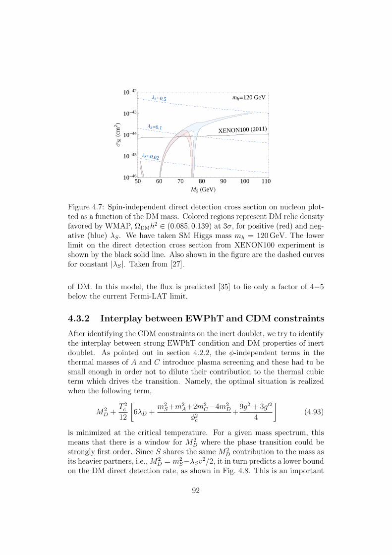
XENON100 H2011L
mh=120 GeVΛS=0.5
ΛS=0.1
ΛS=0.02
50 60 70 80 90 100 11010-46
10-45
10-44
10-43
10-42
MS HGeVL
ΣSI
Hcm
2 L
Figure 4.7: Spin-independent direct detection cross section on nucleon plot-ted as a function of the DM mass. Colored regions represent DM relic densityfavored by WMAP, ΩDMh
2 ∈ (0.085, 0.139) at 3σ, for positive (red) and neg-ative (blue) λS. We have taken SM Higgs mass mh = 120 GeV. The lowerlimit on the direct detection cross section from XENON100 experiment isshown by the black solid line. Also shown in the figure are the dashed curvesfor constant |λS|. Taken from [27].
of DM. In this model, the flux is predicted [35] to lie only a factor of 4−5below the current Fermi-LAT limit.
4.3.2 Interplay between EWPhT and CDM constraints
After identifying the CDM constraints on the inert doublet, we try to identifythe interplay between strong EWPhT condition and DM properties of inertdoublet. As pointed out in section 4.2.2, the φ-independent terms in thethermal masses of A and C introduce plasma screening and these had to besmall enough in order not to dilute their contribution to the thermal cubicterm which drives the transition. Namely, the optimal situation is realizedwhen the following term,
M2D +
T 2c
12
[6λD +
m2S+m2
A+2m2C−4m2
D
φ2c
+9g2 + 3g′2
4
](4.93)
is minimized at the critical temperature. For a given mass spectrum, thismeans that there is a window for M2
D where the phase transition could bestrongly first order. Since S shares the same M2
D contribution to the mass asits heavier partners, i.e., M2
D = m2S−λSv2/2, it in turn predicts a lower bound
on the DM direct detection rate, as shown in Fig. 4.8. This is an important
92
Xenon 100
100 150 200 250 300 350 40010-47
10-46
10-45
10-44
10-43
mC=mA HGeVL
ΣSI
Hcm
2 L
Figure 4.8: Correlation between spin-independent direct detection cross sec-tion and the mass of the charged scalar, after imposing the strong elec-troweak transition condition φc/Tc > 1. We have scanned the parameterspace: mh ∈ (115, 200) GeV, mS ∈ (40, 80) GeV, mA ∈ (100, 500) GeV,mC ∈ (mA − 10 GeV,mA + 10 GeV), λS ∈ (0, 1) and λD ∈ (0, 3). We vetopoints where the thermal mass of A or C exceeds 1.8Tc, which would invali-date the high temperature expansion. Taken from [27].
result in view of the upper bound set by XENON100, which constrains themasses of A and C to lie in a window between 270−350 GeV.
This mass window of heavy scalar masses can be probed by the LHC. Inparticular, the pseudo-scalar component A can be produced in associationwith the DM S, and leads to dilepton final state with missing energy. Here,the preferred mass difference between A and S is larger than the samplevalues studied in [51], which makes it easier to be distinguished from the SMbackground by imposing a harder cut on the missing energy.
Why not a singlet? Before turning to higher representations, let us dis-cuss explicitly the case of the singlet DM. After all, this is a simpler possibilitywith fewer couplings and thus more constrained. In fact, it fails to do the job.More precisely, while the singlet by itself can actually help the phase transi-tion to be of the first order [17], it cannot simultaneously be the DM [210],and vice versa.
What happens is the following. In this case, there is only one couplingwith the Higgs and λA ≡ λC ≡ λS. We survey all the points in Fig. 4.8and find they all satisfy λA,C & 1. On the other hand, direct detection, asshown in Eq. (4.92), constrains this coupling to be much smaller than whatis needed to trigger a strong first-order phase transition. The failure of the
93
real singlet thus makes the choice of the inert doublet scalar the simplestone. One can further extend the real scalar singlet case to a complex one.It was shown [63] that the double job of dark matter and strong electroweakphase transition can be achieved in this case.
4.4 The Quartet/Doublet versus EW, EW-
PhT and CDM constraints.
In this section, we have tried to identify the region of parameter space forhigher representations where one can have a light DM candidate consistentwith other phenomenological constraints along with strong EWPhT. As al-ready pointed out in section (4.1.2), the DM of complex even integer multiplet(Y 6= 0) is excluded by the bound from the direct detection. On the otherhand, the γ term of Eq.(4.1) can split the neutral component of half integerrepresentation and one can easily obtain a light DM component. As quar-tet multiplet (j = 3/2) is the immediate generalization of the inert doublet,we have focused on identifying DM properties in parallel with its impact onstrong EWPhT.
4.4.1 Model parameters scan and constraints
The masses of quartet’s component fields are determined by four free pa-rameters MQ, α, β, γ, Eq.(4.13). But (co)annihilation cross sections whichcontrol the relic density of the dark matter depend on the mass splittingsamong the dark matter and the other components in the multiplet. There-fore we used alternative free parameter set mS, λS,mQ++ ,mA where mS
is the DM mass and λS = α + 14β − 2γ is the coupling between the Higgs
and dark matter component. One can express MQ, α, β, γ,mQ+1,mQ+
2 in
terms of these four parameters using mass relations Eq.(4.13). Moreover, inthe case of quartet, for S to be the lightest component of the multiplet, oneneeds to impose two conditions, γ > 0 and γ ≥ |β|
2which in turn sets the
mass spectrum to be mS < mQ+1< mQ++ < mQ+
2< mA.
Collider constraints:
Direct collider searches at LEP II has put a strong bound on single chargedparticle which is mQ+
1> 70 − 90 GeV [203]. But the doubly charged scalar
of the quartet which only has the cascade decay channel is not stronglyconstrained by collider searches. One constraint can come from W and Zboson width. In our case, setting S as DM imposes in the mass spectrum:
94

mQ++ ≥ mQ+1
, so the constraint on the single charged scalar is also translatedinto a bound on the doubly charged scalar for such mass spectrum. Moreover,the deviations of W and Z width from their SM values can take place throughdecay channels: W± → SQ±1 /AQ
±1 /Q
±±Q∓1 and Z → Q+1 Q−1 /SA/Q
++Q−−.Therefore to avoid such deviation the following mass constraints are alsoimposed: mS +mQ+
1> mW , mA +mQ+
1> mW , mQ++ +mQ+
1> mW , mQ+
1>
mZ/2, mQ++ > mZ/2 and mS + mA > mZ . Apart from collider constraints,one also impose constraints coming from electroweak precision observables.In our scan, we used the allowed range of T parameter, Eq.(4.39) and Sparameter, Eq.(4.41).
DM relic density constraint:
The dark matter density of the universe measured by Planck collaborationis ΩDMh
2 = 0.1196 ± 0.0031 (68% CL) [9]. To determine the relic densityof the multiplets, we used FeynRules [205] to generate the model files forMicrOMEGAs [211]. For inert multiplets, mass splitting between compo-nents are set by both β and γ couplings. In case of doublet, one can setβ and γ to produce large spitting between S component and single chargedcomponent C+ or between S and A in such way that such splitting is compat-ible with electroweak precision observables. Such large splitting can lead tosuppression of co-annihilation channels SA, SC+ → SM particles. But suchsimple tuning of the couplings like in the doublet is not possible for quartetbecause of the mass relation Eq.(4.13). Therefore there is a possibility forco-annihilation channel to open up when mQ+
1/mS ≤ 1.5 ( [204]).
Apart from co-annihilation, other dominant channels which will controlthe relic density of DM at the low mass region are SS → h∗ → bb andSS → WW .
Direct DM detection and invisible Higgs decay constraints:
The updated direct detection limit on the spin independent DM-nucleoncross section is set by XENON100 with 225 days live data [208] where σSI .2 × 10−45cm2. In addition, the future XENON1T will reach the sensitivityof σSI . 2× 10−47cm2 [209].
Also if the mass of the dark matter is smaller than half of the Higgs mass,it will contribute to the invisible decay of the Higgs through h → SS withbranching ratio Brinv = Γinv/(ΓSM + Γinv), where ΓSM = 6.1 MeV and,
Γinv =λ2Sv
2
64πmh
√1− 4m2
S
m2h
(4.94)
95
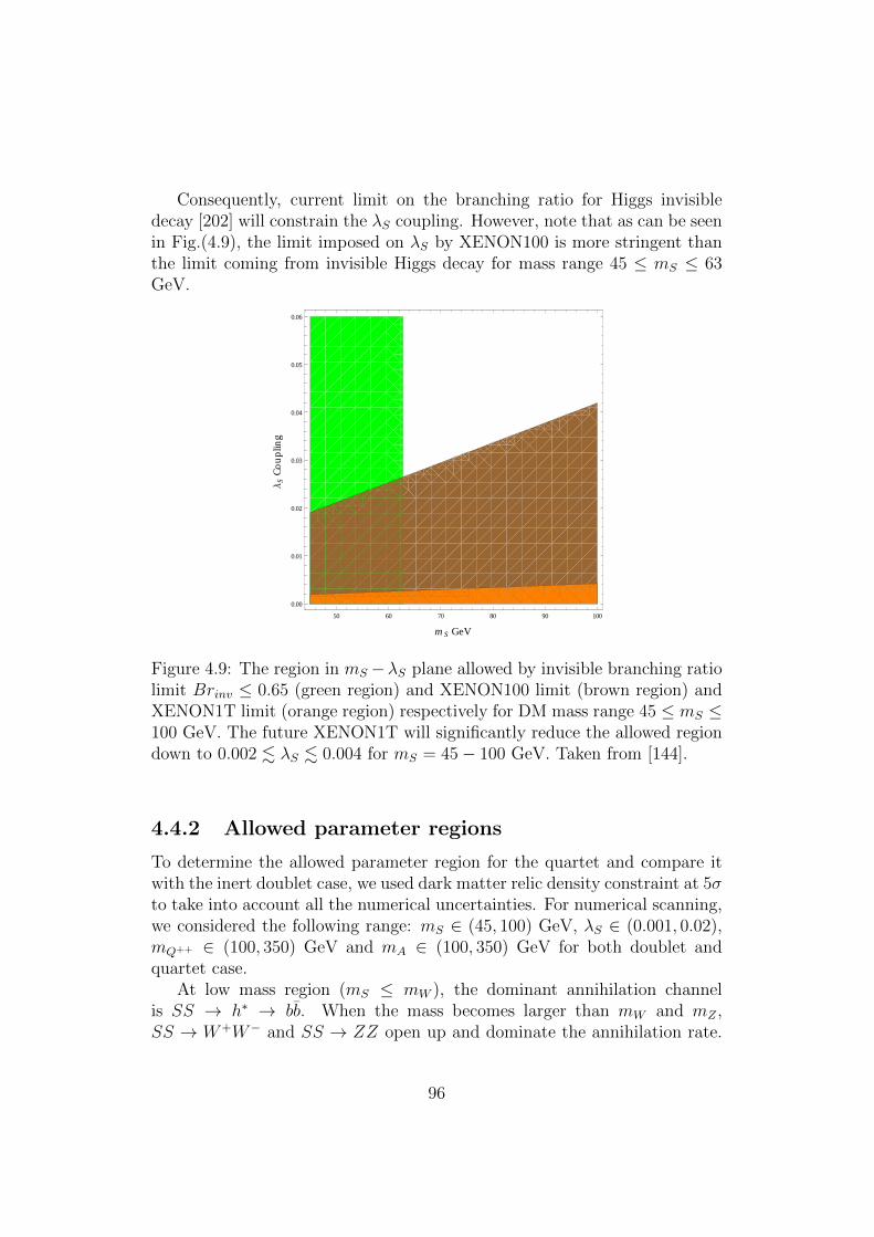
Consequently, current limit on the branching ratio for Higgs invisibledecay [202] will constrain the λS coupling. However, note that as can be seenin Fig.(4.9), the limit imposed on λS by XENON100 is more stringent thanthe limit coming from invisible Higgs decay for mass range 45 ≤ mS ≤ 63GeV.
50 60 70 80 90 100
0.00
0.01
0.02
0.03
0.04
0.05
0.06
mS GeV
ΛS
Co
up
ling
Figure 4.9: The region in mS −λS plane allowed by invisible branching ratiolimit Brinv ≤ 0.65 (green region) and XENON100 limit (brown region) andXENON1T limit (orange region) respectively for DM mass range 45 ≤ mS ≤100 GeV. The future XENON1T will significantly reduce the allowed regiondown to 0.002 . λS . 0.004 for mS = 45− 100 GeV. Taken from [144].
4.4.2 Allowed parameter regions
To determine the allowed parameter region for the quartet and compare itwith the inert doublet case, we used dark matter relic density constraint at 5σto take into account all the numerical uncertainties. For numerical scanning,we considered the following range: mS ∈ (45, 100) GeV, λS ∈ (0.001, 0.02),mQ++ ∈ (100, 350) GeV and mA ∈ (100, 350) GeV for both doublet andquartet case.
At low mass region (mS ≤ mW ), the dominant annihilation channelis SS → h∗ → bb. When the mass becomes larger than mW and mZ ,SS → W+W− and SS → ZZ open up and dominate the annihilation rate.
96
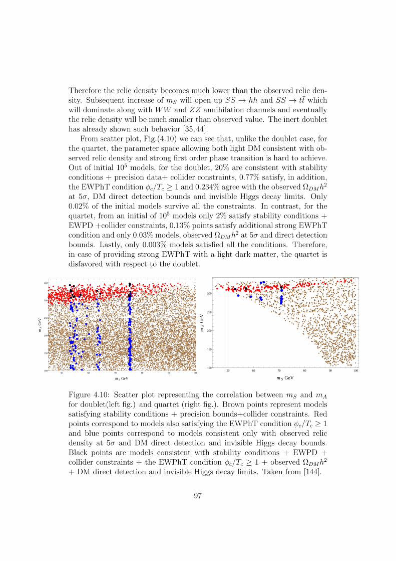
Therefore the relic density becomes much lower than the observed relic den-sity. Subsequent increase of mS will open up SS → hh and SS → tt whichwill dominate along with WW and ZZ annihilation channels and eventuallythe relic density will be much smaller than observed value. The inert doublethas already shown such behavior [35,44].
From scatter plot, Fig.(4.10) we can see that, unlike the doublet case, forthe quartet, the parameter space allowing both light DM consistent with ob-served relic density and strong first order phase transition is hard to achieve.Out of initial 105 models, for the doublet, 20% are consistent with stabilityconditions + precision data+ collider constraints, 0.77% satisfy, in addition,the EWPhT condition φc/Tc ≥ 1 and 0.234% agree with the observed ΩDMh
2
at 5σ, DM direct detection bounds and invisible Higgs decay limits. Only0.02% of the initial models survive all the constraints. In contrast, for thequartet, from an initial of 105 models only 2% satisfy stability conditions +EWPD +collider constraints, 0.13% points satisfy additional strong EWPhTcondition and only 0.03% models, observed ΩDMh
2 at 5σ and direct detectionbounds. Lastly, only 0.003% models satisfied all the conditions. Therefore,in case of providing strong EWPhT with a light dark matter, the quartet isdisfavored with respect to the doublet.
50 60 70 80 90 100100
150
200
250
300
350
mS GeV
mA
GeV
50 60 70 80 90 100100
150
200
250
300
mS GeV
mA
GeV
Figure 4.10: Scatter plot representing the correlation between mS and mA
for doublet(left fig.) and quartet (right fig.). Brown points represent modelssatisfying stability conditions + precision bounds+collider constraints. Redpoints correspond to models also satisfying the EWPhT condition φc/Tc ≥ 1and blue points correspond to models consistent only with observed relicdensity at 5σ and DM direct detection and invisible Higgs decay bounds.Black points are models consistent with stability conditions + EWPD +collider constraints + the EWPhT condition φc/Tc ≥ 1 + observed ΩDMh
2
+ DM direct detection and invisible Higgs decay limits. Taken from [144].
97
4.5 Summary
The combination of the electroweak constraints with the results of EWPhTand dark matter properties for the inert doublet and the quartet has pointedout that the inert quartet provides much smaller region of parameter spacecompared to the doublet in this class of models. Therefore, the inert doubletcan be a more plausible candidate for the dark matter which simultaneouslyprovides strong first order EWPhT in the universe.
98
Chapter 5
Conclusions and outlook
We have considered the electroweak phase transition and dark matter phe-nomenology with various inert scalar representations used for extending theSM’s Higgs sector. The details of the phenomenological studies are done bymaking random scans of parameters within the triplet and quartet context.The results from our analyses in comparing the allowed parameter regions ofthe above mentioned models with the inert doublet model case are summa-rized as follows
• As the size of an inert multiplet which can be added to the SM is notarbitrary but is rather controlled by the perturbativity of SU(2) gaugecoupling at TeV scale (∼ 10 TeV), which sets an upper bound on thesize of the multiplet to be j ≤ 5, that motivated us to study the EWPhT(and subsequently, the DM characteristics) for inert doublet, tripletand quartet models as representatives for allowed larger multiplets.We explicitly showed that it is possible to have strong EWPhT withinthe inert doublet, complex inert triplet and the inert quartet models.
– In case of inert doublet, from Fig.(4.7), we can see that, the strongEWPhT region: mA ≡ mC ∼ 270− 350 GeV.
– For complex triplet, from Fig.(4.4), the 1st order EWPhT occursfor region: m∆++ ∼ 170− 340 GeV.
– For quartet, from Fig.(4.5), first order EWPhT region is: mQ++ ∼200− 275 GeV and mA ∼ 230− 320 GeV.
• Using the expression for the latent heat measure, we have made ageneric study of the impact of higher (than the doublet) scalar multi-plets on the strength of electroweak phase transition. The competitionbetween the number of scalar quasiparticles coupled to EW plasma with
99
large couplings and the screening of those particles resulting from scalarself quartic and gauge boson interaction, which will decouple them fromthe plasma, determines the strength of the transition. The rise and fallof the latent heat with large multiplet, as shown in Fig.(4.6), qualita-tively shows such variation of the EWPhT strength.
• Next we require the simultaneous explanation of EWPhT and the coldDM content of the universe within the doublet and quartet frame. Thetriplet with Y = 2, unlike the half integer representations, is alreadyexcluded by the direct detection limit thus can’t play any viable roleof DM triggering strong EWPhT. For both doublet and quartet cases,we first identified the region of parameter space, out of the randomlyscanned parameter points, which allows both strong EWPhT and alight DM candidate by imposing stability conditions, electroweak pre-cision bounds and corresponding experimental limits. Afterwards Theparameter regions for doublet and quartet that survive all constraintsare compared with each other. Requiring that all the CDM content ofthe universe is explained by the scalar multiplet then, from the scatterplot Fig.(4.10), it can be seen that the quartet has only a very smallallowed parameter space in contrast to inert doublet case. Moreover,the allowed parameter space for having DM with observed relic densityand strong EWPhT in both inert doublet and quartet cases will besignificantly constrained by future XENON1T experiment.
Why higher multiplets are disfavored The above results combined to-gether point out that the higher inert representations are rather disfavoredcompared to the inert doublet. In the case of quartet, when masses of dou-bly charged scalar and pseudoscalar are set to have strong EWPhT (i.e.mQ++ ∼ 200− 275 GeV and mA ∼ 230− 320 GeV), bounds on electroweakprecision variables, specially on T parameter that depends on the mass dif-ferences between the components of the multiplet, makes the mass of oneof the single charged components comparable with the DM mass and thatleads to coannihilation which in turn gives relic density much smaller thanthe observed value. In addition, the mass of that light charged scalar be-comes smaller than the LEP II bound (∼ 90 GeV) when all other constraintsare combined. Larger allowed multiplets j = 5/2, 7/2 also have more thanone single charged scalars and similar situation will arise when different con-straints will be combined. Therefore it is harder to satisfy strong EWPhTcondition, EWPD constraints, collider bounds, observed ΩDMh
2 and DMdirect detection constraints simultaneously for higher representations.
The conclusion is qualitative and only valid within the set of experimental
100
and phenomenological constrains considered. There are however room fordoing more in directions we did not consider here:
• The computational and phenomenological machineries are well withinreach for making detailed quantitative analyses within Bayesian sta-tistical framework. Using strong EWPhT condition and recent resultsfrom relic density measurement, direct and indirect detection limits andcollider constraints from LHC, a comparison between the allowed pa-rameter spaces of inert doublet and quartet can be carried out in thisBayesian framework, in a similar manner to the work done for com-paring different supersymmetric models [212,213] and for comparing asingle versus multi-particle CDM universe hypotheses [214].
• Higher (than doublet) scalar multiplets have relatively more chargedcomponents that couple to the Higgs. As such, they will alter thedecay rate of Higgs going to two photons relative to the SM value[215–220]. Persistence of the apparent (given the large uncertainties)excess in the h→ γγ data will severely constrain the triplet and quartetparameter regions with EWPhT driven by large positive couplings [221,222]. This and similar studies will be interesting for establishing theinert multiplets’ status and/or prospects within collider phenomenologyframework.
• Successful baryogenesis requires CP violation, not only the first orderphase transition. It is easy to imagine new sources of CP violation,but the problem then arises as to whether the new physics behind itaffects the nature of the phase transition. In this sense, new fermionsare more welcome, at least in the perturbative regime, while addingnew scalars is less desirable since they may upset the first order phasetransition. Of course, there is always a large parameter space wherethey are innocuous, since even tiny couplings with the SM particlesmay give enough CP violation.
• Apart from detecting new particles within the mass ranges where theytrigger strong first order electroweak phase transition, one could havea more direct consequence of it in the production of gravitationalwaves [223–226] in the universe.
• Another possibility is the pre-existence of baryon asymmetry in theuniverse. In order to elucidate this possibility, let us recall the problemin the conventional picture: due to the symmetry restoration at hightemperature, the unsuppressed rate of sphaleron transition erase any
101

original B + L asymmetry unless the B − L or any other conservedcharge in the electroweak plasma is non-zero. This, however, is notnecessarily true in the BSM physics with enlarged Higgs sector: gaugesymmetry may get even more broken at high temperature [75,79]. Forthis to happen, it suffices that the cross-term couplings between differ-ent scalar multiplets be negative. It may be worthwhile to investigatethis possibility; however it requires improving the perturbative resultsfor next-to-leading effects which tend to be large [227].
102
Appendix A
Mathematical tools
A.1 Properties of Γ(s) and ζ(s)
In the following we have collected some properties of Γ(s) and ζ(s) that areused in evaluating thermal integrals.
Γ(s) =
∫ ∞0
dxxs−1e−x (A.1)
Γ(s) =Γ(s+ 1)
s(A.2)
Γ′(1) = −γE = −0.57721...
Γ(1
2) =
√π
Γ′(1
2) = −
√π(γE + 2ln2)
Γ(1
2+ ε) =
√π(1− ε(γE + 2ln2) +O(ε2))
Γ(−1
2+ ε) = −2
√π +O(ε) (A.3)
ζ(s) =∞∑n=1
1
sn(A.4)
ζ(0) = −1
2
ζ ′(0) = −1
2ln(2π)
ζ(s) = 2sπs−1 sin(πs
2)Γ(1− s)ζ(1− s) (A.5)
103
For any positive even integer 2n,
ζ(2n) =(−1)n+1(2π)2nB2n
2(2n)!(A.6)
where, B2n are the Bernoulli numbers; B0 = 1, B2 = 1/6, B4 = −1/30,...andB1 = ±1
2, B3 = B5 = 0,...
ζ(2) =π2
6; ζ(3) = 1.202.. ; ζ(4) =
π4
90(A.7)
Moreover, we also have,
ζ(−1 + ε) = − 1
12+O(ε)
ζ(1 + ε) = 21+επε(sinπ
2(1 + ε))Γ(−ε)ζ(−ε)
= −1
ε+ γE +O(ε)
ζ(3 + ε) ∼ ζ(3) +O(ε) ∼ 1.202...+O(ε) (A.8)
A.2 Some useful integrals
I±n =
∫ ∞0
dxxn
ex ± 1(A.9)
I−n − I+n =
∫ ∞0
dxxn2
e2x − 1
=1
2n
∫ ∞0
dyyn
ey − 1
=1
2nI−n
I+n = (1− 1
2n)I−n (A.10)
104
Evaluation of I−n
I−n =
∫ ∞0
dxxn
ex − 1
=
∫ ∞0
dxxne−x(1− e−x)−1
=
∫ ∞0
dx∞∑m=1
xne−mx
=∞∑m=1
1
mn+1
∫ ∞0
dyyne−y
= ζ(n+ 1)Γ(n+ 1) (A.11)
Evaluation by dimensional regularization We define a function f(m,D, n)which is used to evaluate the integrals by dimensional regularization.
f(m,D, n) =
∫dDk
(2π)D1
(k2 +m2)n
=1
(4π)D/2Γ(D/2)
∫ ∞0
(k2)D2−1 1
(k2 +m2)n
=1
(4π)D/2(m2)
D2−nΓ(n− D
2)
Γ(n)(A.12)
When D = 3− ε, we have
f(m, 3− ε, n) =µ−ε
(4π)32
(4πµ2
m2)ε2 (m2)
32−nΓ(n− 3
2+ ε
2)
Γ(n)(A.13)
A.3 Frequency sum
When we deal with loop diagrams in the finite temperature field theory inthe imaginary time formalism, we usually need to evaluate the summationgiven the following
∞∑n=−∞
1
n2 + y2(A.14)
where n is even and odd respectively. First we focus on the even n.Consider a complex function f(z) with the property |f(z)| ≤ M
|z|p where
p > 1 and M is a constant. cot(π2z) has poles at z = 0,±2,±4, ... So the
105
residues of f(z) cot(π2z) at z = n with n even integer and provided f(z) does
not have poles at n,
Resn = limz→n(z − n)cos(π
2z)
sin(π2z)f(z)
=2
πf(n) (A.15)
If f(z) = 1z2+y2 , the poles are z = ±iy will give residues
Res±iy = − iy
cot(iπ
2y) (A.16)
Consider the contour integral where the path C circulates the poles of cot(π2z)
and f(z) so ∫C
f(z) cot(π
2z)dz = 2πi
∑i
Resi (A.17)
But this contour can be deformed so that the integral will be zero. So weimmediately get,
∞∑n=−∞,even
1
n2 + y2=
iπ
2ycot(
iπ
2y)
=π
2ycoth(
π
2y) (A.18)
where coth(x) = i cot(ix) is used.On the other hand, when n = ±1,±3, ..., tan(π
2n) has poles at those
values of n. Therefore, following the same line of arguments, we can derivethat
∞∑n=−∞,odd
1
n2 + y2=
π
2ytanh(
π
2y) (A.19)
We will use the following two simplifications of coth(x) and tanh(x),
coth(x) = 1 +2
e2x − 1(A.20)
tanh(x) = 1− 2
e2x + 1(A.21)
106
Appendix B
Coleman-Weinberg potential
In this appendix, we have collected the expression for the one-loop Cole-man Weinberg (CW) potential in both MS scheme and cut-off regulariza-tion scheme. Here we have presented MS renormalization scheme for zero-temperature one loop Coleman-Weinberg potential as an illustration.
B.1 MS renormalization
From Eq.(2.132), we have
V(1)
CW =
∫dDk
(2π)D
√k2 +m2
2(B.1)
Using Eq.(A.12) and Eq.(A.13) we have,
V(1)SCW =
1
2f(m, 3− ε,−1/2)
=µ−εm4
2(4π)3/2(4πµ2
m2)ε/2
Γ(−2 + ε2)
Γ(−12)
(B.2)
As Γ(−12) = −2
√π and Γ(−2+ ε
2) = 1
ε+ 3
4− γE
2+O(ε), we have from Eq.(B.2)
in the limit ε→ 0,
V(1)SCW = − m4
64π2(2
ε− γE + ln4π) +
m4
64π2(ln
m2
µ2− 3
2) (B.3)
So removing the first term in MS scheme, we have,
V(1)SCW =
m4s(φc)
64π2(ln
m2s(φc)
µ2− 3
2) (B.4)
107
Similarly for fermions, we have from Eq.(2.144) by removing the divergentpart in MS scheme,
V(1)FCW = −2gf
m4f (φc)
64π2(ln
m2f (φc)
µ2− 3
2) (B.5)
On the other hand for the gauge bosons we have
V(1)gbCW = 3
m4gb(φc)
64π2(ln
m2gb(φc)
µ2− 5
6) (B.6)
B.2 CW effective potential in the Standard
Model
Here we collect the expression for one loop CW potential for the StandardModel. The Higgs field of the Standard Model is,
Φ =
G±
φc + h+ iG0
√2
(B.7)
where φc is the real constant background, h the Higgs field, and G± and G0
are the three Goldstone bosons. The tree level potential reads, in terms ofthe background field, as
V0(φc) = −m2
2φ2c +
λ
4φ4c (B.8)
with positive λ and m2, and the tree level minimum corresponding to
v2 =m2
λ.
The field dependent masses of the scalar fields are
m2h(φc) = −m2 + 3λφ2
c
m2G±,G0(φc) = −m2 + λφ2
c (B.9)
so that m2h(v) = 2λv2 = 2m2 and m2
G±,G0(v) = 0. The gauge bosons con-tributing to the one-loop effective potential are W± and Z, with tree levelfield dependent masses,
m2W (φc) =
g2
4φ2c (B.10)
m2Z(φc) =
g2 + g′2
4φ2c
108
Finally, the only fermion which can give a significant contribution to the oneloop effective potential is the top quark, with a field-dependent mass
m2t (φc) =
y2t
2φ2c (B.11)
where yt is the top quark Yukawa coupling.
B.2.1 MS renormalization
In the MS renormalization scheme the finite effective potential for the SM isprovided by
V (φc) = V0(φc) +1
64π2
∑i=W,Z,h,G±,G0,t
nim4i (φc)
[log
m2i (φc)
µ2− Ci
](B.12)
where Ci are constants given by,
CW = CZ =5
6(B.13)
Ch = CG±,G0 = Ct =3
2and ni are the degrees of freedom
nW = 6, nZ = 3, nh = 1, nG±,G0 = 3, nt = −12 (B.14)
B.2.2 Cut-off regularization
A useful cut-off regularization scheme was presented in [17] where the fol-lowing two conditions are imposed:
• the tree level minimum is preserved at one loop.
• At one loop, tree level value of the Higgs mass is also preserved
or in other words,
d(V1 + Vct)
dφc
∣∣∣∣φc=v
= 0 (B.15)
d2(V1 + Vct)
dφ2c
∣∣∣∣φc=v
= 0
where V1 is the one loop effective potential and Vct is the counter-term po-tential to remove the divergences. The final result is [17,84],
V (φc) = V0(φc) +1
64π2
∑i
m4i (φc)
(log
m2i (φc)
m2i (v)
− 3
2
)+ 2m2
i (v)m2i (φc)
(B.16)
109
Appendix C
High and low temperatureexpansion
C.1 Limits of thermodynamic quantities
The high and low temperature limits, which is also called relativistic andnon-relativistic limits follow mi/T 1 and mi p, T respectively.
For convenience at first we present the following two results from sectionA.2 which are going to used for evaluating momentum integrals. The integralsare
I±n =
∫ ∞0
dxxn
ex ± 1(C.1)
I+n = (1− 1
2n)I−n (C.2)
I−n = ζ(n+ 1)Γ(n+ 1) (C.3)
Now let us consider first Eq.(2.11) in the relativistic limit,
nB =1
2π2
∫ ∞0
p2dp1
ep/T − 1
=T 3
2π2
∫ ∞0
dxx2
ex − 1replacing x = p/T
=ζ(3)
π2T 3 (C.4)
Using Eq.(C.2) we have for number density for fermionic case,
nF =3
4
ζ(3)
π2T 3 (C.5)
110
Here, ζ(3) = 1.202.. is the Riemann zeta function. If the degrees of freedomfor bosons and fermions are gB and gF respectively, we have the total numberdensity in the relativistic limit,
n = (gB +3
4gF )
ζ(3)
π2T 3 (C.6)
For example, for photons, gB = 2, for real(complex) scalar, gB = 1(2) andfor Majorana(Dirac) fermion, gF = 4(2).
Now let us consider the relativistic limit for the energy density. FromEq.(2.13), we can see that there are two contributions. The first term isthe zero temperature one-loop Coleman Weinberg potential and second termrepresents the finite temperature part. Focusing on second term, again inthe relativistic limit, we have from Eq.(2.13),
ρB =1
2π2
∫ ∞0
p2dpp
ep/T − 1
=T 4
2π2
∫ ∞0
dxx3
ex − 1
=π2
30T 4 (C.7)
Similarly again using Eq.(C.2), we have for fermionic case,
ρF =7
8
π2
30T 4 (C.8)
So the total energy density in the relativistic limit is
ρ = (gB +7
8gF )
π2
30T 4 (C.9)
Now let us consider the non-relativistic case where m p, T . In thislimit,
n =1
2π2
∫ ∞0
p2dpe−√
(p2+m2)/T 2
=T 3
2π2
∫ ∞0
dxx2e−√x2+y2
; y = m/T
=T 3
π2
∫ ∞y
dzz√z2 − y2e−z ;x2 = z2 − y2
=T 3
π2
√2y
32 e−y
∫ ∞0
dvv12 e−v ; v = z + y
=
(mT
2π
)3/2
e−m/T (C.10)
111
And the energy density in non-relativistic case is
ρB = ρF = mn (C.11)
We can see that, the contribution of non-relativistic spices in the numberand energy densities is very small compared to the relativistic particles.
Let us now consider the entropy and the free energy of in the relativisticlimits. From Eq.(2.16), the first term has turned out to be,
sB1 =π2
30T 3 (C.12)
The second term of entropy in Eq.(2.16) is evaluated in the following way.In the relativistic limit, we can write it as
sB2 =1
2π2
∫ ∞0
dp p2ln(1− e−p/T ) (C.13)
So we can have,
∂sB2
∂T= − 1
2π2T 2
∫ ∞0
dpp3
ep/T − 1
= − T 2
2π2
∫ ∞0
dxx3
ex − 1
= − T 2
2π2ζ(4)Γ(4) = −π
2
30T 2
So we have
sB2 = −π2
90T 3 (C.14)
By adding two pieces,
sB =2π2
45T 3 (C.15)
In case of fermion, the entropy density is
sF =2π2
45
7
8T 3 (C.16)
Therefore the total entropy density of the system will be
s =2π2
45T 3(gB +
7
8gF ) (C.17)
Finally let us address the free energy density in the relativistic limit.From Eq.(2.19), considering only the temperature dependent part, we have,
fB =T
2π2
∫ ∞0
dp p2ln(1− e−p/T ) (C.18)
112
Following the same steps for Eq.(C.13), we have
fB = −π2
90T 4 (C.19)
So now the total free energy density and the pressure of a system with bosonsand fermions is,
f = −p = −π2
90T 4(gB −
7
8gF ) (C.20)
C.2 High temperature expansion for the toy
model
In this section we have presented the derivation of high temperature limit ofscalar and fermionic contribution to scalar self energy and find out the Debyescreening which occurs at finite temperature. The high temperature limit isthe condition, mi/T 1. First we consider bosonic contribution.
δ(B)m2T =
λ
2
∫d3k
(2π)3
1
ωk
1
eωk/T − 1
=λT 2
4π2
∫dx
x2√x2 +m2/T 2
1
e√x2+m2/T 2 − 1
At the high temperature limit it is reduced to
δ(B)m2T =
λT 2
4π2
∫ ∞0
dxx
ex − 1=λT 2
4π2ζ(2)Γ(2)
=λT 2
24(C.21)
Following similar steps for fermion loop, we have,
δ(F )m2T =
2y2φT
2
π2
∫ ∞0
dxx
ex + 1
= y2φ
T 2
6(C.22)
Therefore the Debye screening is,
Π(T ) = (λ
2+ 2y2
φ)T 2
12(C.23)
113
C.3 High and low temperature expansion of
the effective potential
The high and low temperature expansion of the finite temperature effectivepotential is done following [85]. Let us first consider the bosonic finite tem-perature effective potential.
C.3.1 Bosonic high temperature expansion
The starting expression for the bosonic effective potential is
V Teff(φc) = T
∞∑n=−∞
∫d3k
(2π)3ln(4π2n2T 2 + ~k2 +m(φc)
2)
= T∞∑
n=−∞
∫d3k
(2π)3ln(4π2n2T 2 + ω2) (C.24)
Therefore let us define,
J(m,T ) = T∞∑
n=−∞
∫dDk
(2π)Dln(4π2n2T 2 + k2 +m2) (C.25)
And,
H(m,T ) = T∞∑
n=−∞
∫dDk
(2π)D1
4π2n2T 2 + k2 +m2(C.26)
From Eq.(C.25) and Eq.(C.26) we can see that,
H(m,T ) =1
m
d
dmJ(m,T ) (C.27)
J(m,T ) =
∫ m
0
dm′m′H(m′, T ) (C.28)
Let us start from Eq.(C.26). The zero mode contribution n = 0 to theEq.(C.26) can be evaluated using f(m, 3− ε, 1) in the limit ε→ 0 as follows,
H(n=0)(m,T ) = Tf(m, 3− ε, 1)
= Tm
(4π)32
Γ(−1/2) = −mT4π
(C.29)
114
Now we focus on the contributions of non-zero modes in the integralEq.(C.26).
H(n 6=0)(m,T ) = T∑n
∫dDk
(2π)D1
(2πnT )2 + k2 +m2
= 2T∞∑n=1
∫dDk
(2π)D1
(2πnT )2 + k2(1 +
m2
(2πnT )2 + k2)−1
= 2T∞∑n=1
∞∑l=0
∫dDk
(2π)D(−1)l
m2l
((2πnT )2 + k2)l+1
=2T
(4π)D/21
(2πT )2−D
∞∑l=0
(−1)lm2l
(2πT )2l
∞∑n=1
1
n2l+1−D
=2T
(4π)D/21
(2πT )2−D
∞∑l=0
(−1)lm2l
(2πT )2lζ(2l + 1−D)(C.30)
Now evaluating Eq.(C.30) for D = 3− ε gives,
H(n6=0) =µ−εT 2
√4π
(4πµ2
4π2T 2)ε2
∞∑l=0
(−1)l(m2
4π2T 2)l
Γ(l − 12
+ ε)
Γ(l + 1)ζ(2l−1+ε) (C.31)
In the following we have evaluated H(n6=0) for l = 0 and l = 1 respectively.
H(n6=0)l=0 =
µ−εT 2
√4π
(4πµ2
4π2T 2)ε2 Γ(−1
2+ ε)ζ(−1 + ε)
=T 2
2√π
Γ(1
2)ζ(−1)
=T 2
12(C.32)
H(n6=0)l=1 = −µ
−εT 2
√4π
(4πµ2
4π2T 2)ε2m2
4π2T 2
Γ(12
+ ε2)
Γ(2)ζ(1 + ε)
= −µ−εm2
8π2(1 +
ε
2ln
4πµ2
4π2T 2)(
1
ε+γE2− 1
2ln4)
= − m2
8π2ε− m2
8π2lnµeγE
4πT; (µ2 = 4πµ2/eγE) (C.33)
where we have used
Γ(1
2+ε
2)ζ(1 + ε) =
√π(
1
ε+γE2− 1
2ln4 +O(ε)) (C.34)
115
Now by using dimensional regularization again, we get the zero temper-ature contribution to H(m,T )
H0(m) =
∫dDk
(2π)D1
2√k2 +m2
=1
2f(m, 3− ε, 1
2)
=µ−εm2
2(4π)32
(4πµ2
m2)ε2
Γ( ε2− 1)
Γ(12)
=µ−εm2
2(4π)32
(1 +ε
2ln
4πµ2
m2)
1√π
(−2
ε+ γE − 1 +O(ε))
= − m2
8π2ε− m2
8π2lnµ
m− m2
16π2(C.35)
Now the bosonic thermal integral is
H(m,T ) =T 2
12− mT
4π− m2
8π2ε− m2
8π2lneγE µ
4πT
+T 2
2√π
∞∑l=2
(−1)l(m2
4π2T 2)l
Γ(l − 12)
Γ(l + 1)ζ(2l − 1) (C.36)
Therefore the thermal contribution to the bosonic integral, Eq.(C.26) is
HT (m,T ) = H(m,T )−H0(m)
=T 2
12− mT
4π− m2
8π2ε− m2
8π2lneγE µ
4πT
+T 2
2√π
∞∑l=2
(−1)l(m2
4π2T 2)l
Γ(l − 12)
Γ(l + 1)ζ(2l − 1)
+m2
8π2ε+m2
8π2lnµ
m+
m2
16π2(C.37)
Therefore we have
HT (m,T ) =T 2
12− mT
4π− m2
8π2(ln
m
4πe−γET− 1
2)
+T 2
2√π
∞∑l=2
(−1)l(m2
4π2T 2)l
Γ(l − 12)
Γ(l + 1)ζ(2l − 1) (C.38)
116
From Eq.(C.38) we have,
JT (m,T ) =
∫ m
0
dm′m′HT (m,T )
=m2T 2
24− m3T
12π− m4
64π2(ln
m2
16π2e−2γET 2− 3
2)
+m2T 2
4√π
∞∑l=2
(m2
4π2T 2)l
Γ(l − 12)
Γ(l + 2)ζ(2l − 1) (C.39)
C.3.2 Fermionic high temperature expansion
Let us now focus on the high temperature expansion of the fermionic effectivepotential. In bosonic case, we encounter frequency sum of the following form,
σb(T ) = T∞∑
n=−∞
f(ωn) (C.40)
where f(ωn) = 1ω2n+ω2 with ωn = 2πnT and ω2 = k2 +m2.
On the other hand, for fermionic cases, the frequency sum is
σf (T ) = T∞∑
n=−∞
f(ωn) (C.41)
where ωn = (2n + 1)πT . In the following we are going to recast fermionicsum in terms of bosonic sum, Eq.(C.40).
σf (T ) = T [...+ f(−3πT ) + f(−πT ) + f(πT ) + ...]
= T [...+ f(−3πT ) + f(−2πT ) + f(−πT ) + f(0) + f(πT ) + f(2πT )...]
− T [...+ f(−2πT ) + f(0) + f(2πT ) + ...]
= 2T
2[...+ f(−6π
T
2) + f(−4π
T
2) + f(−2π
T
2) + f(0) + f(2π
T
2) + f(4π
T
2)...]
− T [...+ f(−2πT ) + f(0) + f(2πT ) + ...]
= 2σb(T
2)− σb(T ) (C.42)
Using Eq.(C.42), the fermionic thermal integrals can be evaluated using the
117
results of bosonic thermal integrals.
H(m,T ) = T∑n
∫d3k
(2π)3
1
(2n+ 1)2π2T 2 + k2 +m2
=
∫d3k
(2π)3σf (T )
=
∫d3k
(2π)3
[2σb(
T
2)− σb(T )
]= 2H(m,
T
2)−H(m,T ) (C.43)
Now using Eq.(C.36), we have
H(m,T ) = −T2
24− m2
8π2ε− m2
8π2lneγE µ
4πT− m2
8π2ln4
− T 2
2√π
∞∑l=2
(−1)l(1− 22l−1)(m2
4π2T 2)l
Γ(l − 12)
Γ(l + 1)ζ(2l − 1)(C.44)
The thermal contribution to the fermionic integral is
HT (m,T ) = H(m,T )−H0(m) (C.45)
HT (m,T ) = −T2
24−m
2
8π2lneγEm
πT− T 2
2√π
∞∑l=2
(−1)l(1−22l−1)(m2
4π2T 2)l
Γ(l − 12)
Γ(l + 1)ζ(2l−1)
(C.46)Therefore, from Eq.(C.46), the fermionic integral is determined as follows
JT (m,T ) =
∫ m
0
dm′m′HT (m′, T ) (C.47)
JT (m,T ) = −m2T 2
48− m4
64π2(ln
m2
π2e−2γET 2− 3
2)
− m2T 2
4√π
∞∑l=2
(−1)l(1− 22l−1)(m2
4π2T 2)l
Γ(l − 12)
Γ(l + 2)ζ(2l − 1)(C.48)
118
C.3.3 Low temperature expansion
In this section we will consider the case, m T . Denoting y = m/T 1we have in such limit,
JT (m,T ) =
∫ ∞0
dxx2ln(1− e−√x2+y2
)
= −∫ ∞
0
dxx2e−√x2+y2
+O(e−2y)
=
∫ ∞y
dzz√z2 − y2e−z +O(e−2y)
= −e−y∫ ∞
0
dv(v + y)√v2 + 2vye−v +O(e−2y)
= −√
2y32 e−y
∫ ∞0
dvv12 e−v(1 +
v
y)(1 +
v
4y) +O(e−2y)
= −√
2y32 e−yΓ(
3
2)(1 +O(
1
y) +O(e−y)) (C.49)
Therefore we have,
VT = −T 4(m
2πT)
32 e−
mT (1 +O(
T
m) +O(e−
mT ) (C.50)
and
HT (m,T ) =T 3
m(m
2πT)
32 e−
mT (1 +O(
T
m) +O(e−
mT ) (C.51)
Therefore the high temperature expansion of thermal effective potentialEq.(2.149), we have
VT (φc) =∑B
gB
[m2B(φc)T
2
12− m3
B(φc)T
12π− m4
B(φc)
64π2
(lnm2B(φc)
abT 2− 3
2
)]+
∑F
gF
[m2F (φc)T
2
48+m4F (φc)
64π2
(lnm2F (φc)
afT 2− 3
2
)](C.52)
where, ab = 16π2e−2γE and af = π2e−2γE .
119
Appendix D
Asymptotic limits of thesphaleron field profiles
To capture the dependence of solutions on (J, Y ), in this section we haveincluded the analytical estimates of solutions for the asymptotic region ξ → 0and ξ →∞.
For the energy functional Eq.(3.48) to be finite, the profile functionsshould be f(ξ) → 0, f3(ξ) → 0, f0(ξ) → 1 and h(ξ) → 0. Therefore, atξ ∼ 0, the equations Eq.(3.50) are reduced into
ξ2f ′′ − 4f + 2f3 + αξ2h2 = 0 (D.1)
ξ2f ′′3 − 6f3 + 4f + βξ2h2 = 0 (D.2)
f ′′0 + 2(1− f0)− (g′
g)2βξ2h2 = 0 (D.3)
ξ2h′′ + 2ξh′ − 8m
3h = 0 (D.4)
where
m =Ω2
v2(2α + β) (D.5)
The solution of Eq.(D.4) which leads to the finite energy of the sphaleronis
h(ξ) ∼ Aξ−12
(1−p) (D.6)
where
p =
√1 +
32
3m (D.7)
Now at ξ ∼ 0, f(ξ) ∼ f3(ξ), so using this approximation, from Eq.(D.1)we have,
f(ξ) ∼ Bξ2 − 4Aαξ12
(3+p)
(p2− 1)(p
2+ 5)
(D.8)
120
On the other hand, we have considered f(ξ) as a perturbation in Eq.(D.2).Therefore, we have
f3(ξ) ∼ Cξ3 +Bξ2 −Kξ12
(3+p) (D.9)
Here, K is defined as follows,
K =k1
k2
(D.10)
k1 = 3A3α(3p− 8m+ 3) + 8mβ(4m− 9) (D.11)
k2 = 4m(4m− 9)(8m+ 3p− 15) (D.12)
Finally from Eq.(D.3), we have
f0(ξ) ∼ 1 +Dξ2 +3Aβn2
1ξ12
(3+p)
3p− 8m+ 3(D.13)
where n1 = g′/g.Here, A, B, C and D are the integration constants.On the other hand, for asymptotic region, ξ ∼ ∞, all the profile functions
must approach unity to have finite energy of the sphaleron. So we considerthe functions to be the small perturbation to unity as follows. Taking, f(ξ) =1 + δf(ξ), f3(ξ) = 1 + δf3(ξ), f0(ξ) = 1 + δf0(ξ) and h(ξ) = 1 + δh(ξ) andkeeping only the linear terms of the variation, we have
δf ′′ − αδf = 0 (D.14)
δf ′′3 + β(δf0 − δf3) = 0 (D.15)
δf ′′0 −g′2
g2β(δf0 − δf3) = 0 (D.16)
ξ2δh′′ − 2ξδh− 3λv2
g2Ω2ξ2δh = 0 (D.17)
The asymptotic solutions at ξ ∼ ∞ are,
f(ξ) ∼ 1 + Ee−√αξ (D.18)
f3(ξ) ∼ 1 + Fe−√βξ (D.19)
f0(ξ) ∼ 1 +Ge−√βξ (D.20)
h(ξ) ∼ 1 +He−
√3λvgΩ
ξ
ξ(D.21)
where E, F , G and H are again integration constants. The constants from Ato H depend on (J, J3) and couplings and they are determined by matching
121
the corresponding asymptotic solutions and their first derivatives at ξ = 1.Therefore after the matching, the integration constants are,
H = −12(p− 1)e
vΩn
12(p+ 1) + v
Ωn
(D.22)
A = 1 +He−vΩn (D.23)
where, n =√
3λg
The constants B and E are given as,
E = − e√α
√α + 2
(2 +2Aα(1− p)
(p2− 1)(p
2+ 5)
) (D.24)
B = 1 + Ee−√α +
4Aα
(p2− 1)(p
2+ 5)
(D.25)
Again the constants C and F are in the following,
F =e√β
√β + 3
(−3 +B − 1
2(3− p)K) (D.26)
C = 1 + Fe−√β −B +K (D.27)
And finally D and G are given as
G =e√β
√β + 2
3Aβn21(1− p)
2(3p+ 8m− 3)(D.28)
D = Ge−√β − 3Aβn2
1
3p+ 8m− 3(D.29)
122
Appendix E
Quartet SU(2) representation
E.1 SU(2) generators in the quartet
The generators R(T a) in representation R of SU(2) are taken in such away that they satisfy the following relation: Tr[R(T a)R(T b)] = T (R)δab.Here T (R) is the dynkin index for the corresponding representation. It isobtained from T (R)D(Ad) = C(R)D(R) where dimension of Adjoint reps.is D(Ad) = 3 for SU(2) and Casimir invariant is
∑aR(T a)R(T a) = j(j + 1)
and dimension of the reps. R is D(R) = 2j + 1. For SU(2) reps. T (12) = 1
2
and T (32) = 5.
The explicit form of the generators for quartet reps are the following:
T 1 =
0
√3
20 0√
32
0 1 0
0 1 0√
32
0 0√
32
0
, T 2 =
0 −
√3i2
0 0√3i2
0 −i 0
0 i 0 −√
3i2
0 0√
3i2
0
, T 3 = diag(3
2,1
2,−1
2,−3
2).
(E.1)The raising and lowering operators are defined as T± = T 1 ± iT 2. Theantisymmetric matrices in doublet reps is ε and the similar antisymmet-ric matrix for quartet representation, C is constructed using the relationCT aC−1 = −T aT because the explicit form of it depends on the matrixrepresentation of the corresponding generators:
ε =
(0 1−1 0
), C =
0 0 0 10 0 −1 00 1 0 0−1 0 0 0
(E.2)
123
E.2 Gauge-scalar-scalar vertices
In this section we have collected the gauge-scalar-scalar vertices in the quartetsector needed for the electroweak precision observables. All the momenta aretaken inward.
Q++(p1)Q−1 (p2)W−µ :
ie
sw
√3
2cos θ(p1 − p2)µ (E.3)
Q++(p1)Q−2 (p2)W−µ :
ie
sw
√3
2sin θ(p1 − p2)µ (E.4)
Q+1 (p1)S(p2)W−
µ :ie
2sw(2 cos θ +
√3 sin θ)(p1 − p2)µ (E.5)
Q+1 (p1)A(p2)W−
µ :e
2sw(2 cos θ −
√3 sin θ)(p1 − p2)µ (E.6)
S(p1)Q+2 (p2)W−
µ :ie
2sw(√
3 cos θ − 2 sin θ)(p1 − p2)µ (E.7)
A(p1)Q+2 (p2)W−
µ : − e
2sw(√
3 cos θ + 2 sin θ)(p1 − p2)µ (E.8)
Q++(p1)Q−−(p2)Zµ :ie
2swcw(3c2
w − s2w)(p1 − p2)µ (E.9)
Q+1 (p1)Q−1 (p2)Zµ :
ie
2swcw(2c2
w − cos 2θ)(p1 − p2)µ (E.10)
Q+2 (p1)Q−2 (p2)Zµ :
ie
2swcw(2c2
w + cos 2θ)(p1 − p2)µ (E.11)
S(p1)A(p1)Zµ : − e
2swcw(p1 − p2)µ (E.12)
Q+1 (p1)Q−2 (p2)Zµ : − ie
2swcwsin 2θ(p1 − p2)µ (E.13)
(E.14)
Q++(p1)Q−−(p2)Aµ : 2ie(p1 − p2)µ (E.15)
Q+1 (p1)Q−1 (p2)Aµ : ie(p1 − p2)µ (E.16)
Q+2 (p1)Q−2 (p2)Aµ : ie(p1 − p2)µ (E.17)
124
Appendix F
Tree-Unitarity
The tree-unitarity condition presented in section 4.1.3 is derived here basedon [228, 229]. The S-matrix of the give process can be decomposed in thefollowing way,
S = I + iT (F.1)
where T is the transfer matrix containing the information of the interaction.The unitarity of S-matrix implies
S†S = SS† = I (F.2)
which gives,
T − T † = iT †T
= iTT † (F.3)
where the two equivalent relations arises due to S†S and SS†. If the initialand final states (also considering them to be orthonormal) are denoted as |i〉and |f〉, then we have,
〈f |T |i〉 = i(2π)4δ4(Pf − Pi)Tfi (F.4)
where Pi and Pf are the initial and final total 4-momenta respectively. Sowe have,
Tfi − T ∗if = i(2π)4∑n
δ4(Pf − Pn)TfnT∗in
= i(2π)4∑n
δ4(Pf − Pn)T ∗nfTni (F.5)
where n are the intermediate multiparticle states. To characterize a state, onecan use the total angular momentum J , it’s projection along z-component
125
Jz and the helicity operator Λ = ~J.p because they are conserved quantitiestherefore serve as good quantum numbers.
Consider for simplicity the elastic scattering A + B → A + B in thecenter of mass frame. At first the states are labeled by momentum andhelicity: initial two particle state is |i〉 = |pa, λa; pb, λb〉 and final two particlestate is |f〉 = |p′a, λ′a; p′b, λ′b〉. In the center of mass frame, the 3-momenta of|i〉 are ~pa = −~pb = ~pi. Similarly the 3-momenta in the final state |f〉 are~p ′a = −~p ′b = ~pf .
As the helicity is the component of the spin along the direction of mo-mentum, if we now consider the two particle state as a single particle withhelicity Λ in ~pi direction, then Λ = λa − λb. Similarly for final state, wehave Λ′ = λ′a − λ′b along ~pf direction. Now consider, ~pi is along the z axisand ~pf has the polar angles φ and θ with respect to this fixed coordinatesystem. The rotation matrix Rfi, which is the product of the rotation ofangle θ about y axis and the rotation of angle φ about z axis, transformspi ≡ z into the unit vector p′a = ~p ′a
|~p ′a|.
For the case of 2→ 2 elastic scattering, only 2 particle intermediate stateswill contribute in the summation. Therefore the summation over these statesin Eq.(F.20) will be the integration over the intermediate 3-momenta ~p1 and~p2 and summation over the spin quantum numbers or the helicities of thetwo particles denoted by λ1 and λ2. Also in the CM frame of this system,~p1 = −~p2 = ~pk. ∑
n
→∫
d3~p1
(2π)32E1
d3~p2
(2π)32E2
∑λ1,λ2
(F.6)
The rotation matrix Rki(φ′, θ′, 0) takes ~pi into ~pk and Rkf (φ
′′, θ′′, 0) takes~pf into ~pk. Also, Rki = RkfRfi. Now combining with the delta function wehave∑λ1,λ2
∫d3~p1
(2π)32E1
d3~p2
(2π)32E2
(2π)4δ4(p1 + p2 − Pf ) =1
32π2sλ1/2(s,m2
a,m2b)dΩk
(F.7)with λ(x1, x2, x3) = (x2
1 + x22 + x2
3)2 − 2x1x2 − 2x2x3 − 2x3x1 and dΩk =sin θ′′dθ′′dφ′′.
For any two particle system |p1, λ1; p2, λ2〉, we have ~p1 = −~p2 = ~p in theCM frame and helicity Λ = λ1 − λ2. Moreover, the rotation Rθ,φ transformsz into p direction with polar angles θ and φ. So in this case, the state of totalangular momentum J with M being it’s component in z axis is given by
|J,M ;λ1, λ2〉 =
√2J + 1
4π
∫dφ sin θ dθDJλ1−λ2,M
(R−1θ,φ)|p1, λ1; p2, λ2〉 (F.8)
126
The Wigner’s D-matrix is defined as
DJm′,m(α, β, γ) = 〈J,m′|e−iαJze−iβJye−iγJz |J,m〉 (F.9)
Here, α, β and γ are the Euler angles and Ji are the generators of the rotationgroup. As the helicity is a conserved under rotation, using the Wigner-Eckarttheorem, we have
Tfi = 〈p′a, λ′a; p′b, λ′b|T |pa, λa; pb, λb〉= 16π
∑J
(2J + 1)〈λ′a, λ′b|T J(s)|λa, λb〉DJ∗λa−λb,λ′a−λ′b(φ, θ, 0)(F.10)
Therefore, expanding the LHS of Eq.(F.5) in angular momentum states,
16π∑J
(2J + 1)[〈λ′a, λ′b|T J(s)|λa, λb〉DJ∗λa−λb,λ′a−λ′b(Rfi)
− 〈λ′a, λ′b|T †J(s)|λa, λb〉DJλ′a−λ′b,λa−λb(Rfi)]
= 16π∑J
(2J + 1)[〈λ′a, λ′b|T J(s)|λa, λb〉 − 〈λ′a, λ′b|T †J(s)|λa, λb〉]×
DJ∗λa−λb,λ′a−λ′b(Rfi) (F.11)
where symmetry property, DJm′m(R) = DJ∗
mm′(R) is used. Now the RHS ofEq.(F.5) gives,
i8λ1/2(s,m2
a,m2b)
s
∑J,J ′
∑λ1,λ2
(2J + 1)(2J ′ + 1)〈λ′a, λ′b|T †J(s)|λ1, λ2〉 〈λ1, λ2|T J(s)|λa, λb〉
×∫dΩkDJλ1−λ2,λ′a−λ′b
(Rkf )DJ′∗
λa−λb,λ1−λ2(Rkf )DJ
′∗λa−λb,λ1−λ2
(Rfi)
where we have used, DJm′m(R2.R1) = DJ
m′m(R2)DJm′m(R1). Now using∫
dφ sin θ dθDJ∗m1m2(R)DJ ′m′1m′2(R) =
4π
2J + 1δJJ ′δm′1m1
δm′2m2(F.12)
we have the RHS as follows,
i32πλ1/2(s,m2
a,m2b)
s
∑J
(2J + 1)|〈λ′a, λ′b|T J(s)|λa, λb〉|2DJ∗λa−λb,λ′a−λ′b(Rfi)
(F.13)Therefore, equating both sides and picking up J-th contribution,
〈λ′a, λ′b|T J(s)|λa, λb〉 − 〈λ′a, λ′b|T †J(s)|λa, λb〉
=2iλ1/2(s,m2
a,m2b)
s|〈λ′a, λ′b|T J(s)|λa, λb〉|2(F.14)
127
In the high energy limit, when the masses of the particles can be neglected,from Eq.(F.14), by taking absolute value we have,
|ImT J | ≥ |T J |2 = (ImT J)2 + (ReT J)2 (F.15)
where we have suppressed the helicity indices. The unitarity of S matriximplies |T J | ≤ 1. Therefore by re-arranging Eq.(F.15) we have,
(ReT J)2 ≤ |ImT J |(1− |ImT J |) ≤ 1
4(F.16)
which yields the bound,
|ReT J | ≤ 1
2(F.17)
In case of spinless particles, DJ00(0, θ, 0) = PJ(cos θ) and T J ≡ aJ . PJ(cos θ)
is the Legendre polynomial with θ -the scattering angle. So, Eq.(F.10) re-duces to
Tfi(s, cos θ) = 16π∑J
(2J + 1)aJ(s)PJ(cos θ) (F.18)
Therefore using the orthogonality of the Legendre polynomial∫ 1
−1
d(cos θ)PJ(cos θ)PJ ′(cos θ) =2
2J + 1δJJ ′ (F.19)
we have,
aJ(s) =1
32π
∫ 1
−1
d(cos θ)PJ(cos θ)Tfi(s, cos θ) (F.20)
Since a0 is real in the Born approximation, we can put the bound Eq.(F.17)as the following,
Re a0 ≤1
2(F.21)
This is the desired tree unitarity condition.
128
Appendix G
Renormalization groupequations
Besides the standard diagrammatic methods available to calculate one loop[155] and two loop [156–158], here we are going to describe briefly a simpleand straightforward algebraic method [159, 160] to determine one loop betafunctions for scalar couplings from one loop effective potential.
Consider the one loop effective potential,
Veff = V0 + V1 (G.1)
where for simplicity, we have considered Z2 invariant scalar potential,
V0 = λ1(φ†φ)2 + λ2(χ†χ)2 + αφ†φχ†χ+ βφ†τaφχ†τaχ
+ γ[(φT ετaφ)†(χT ετaχ) + c.c] (G.2)
where φ and χ are the SU(2) doublets. Moreover, τa are the generators ofSU(2) and ε is an antisymmetric matrix in the following,
ε =
(0 −11 0
)(G.3)
The scalar potential written in the form above can be generalized to thelarger scalar multiplets.
The one-loop correction is given by,
V1 =1
64π2STrM4ln
M2
µ2(G.4)
where STr is the spin-weighted trace.
129
In the Landau gauge, the effective potential follows the following equation,[µ∂
∂µ+∑i
βλi∂
∂λi− (γiξi
∂
∂ξi+ c.c)
]Veff = 0 (G.5)
Here, λi = λ1, λ2, α, β, γ and βλi are the associated beta functions. Also,ξi = φ, χ and γi = γφ, γχ are the anomalous dimensions.
At one loop level,
D(1)V0 = −µ∂V1
∂µ=
1
32π2STrM4 (G.6)
where for n-th loop order,
D(n) =∑i
β(n)λi
∂
∂λi− (γ
(n)i ξi
∂
∂ξi+ c.c) (G.7)
If we know anomalous dimensions γi, we can determine all the one loopbeta functions by comparing different quartic terms in the both sides ofEq.(G.6). Therefore let us focus on calculating the mass matrices for differentfields.
For the scalar fields, the squared mass matrix is given by,
M2S =
(A BC D
)(G.8)
where
A =
(∂2V0
∂φi∂φ†j∂2V0
∂φi∂χ†j
∂2V0
∂χi∂φ†j∂2V0
∂χi∂χ†j
)(G.9)
B =
(∂2V0
∂φi∂φj
∂2V0
∂φi∂χj∂2V0
∂χi∂φj
∂2V0
∂χi∂χj
)(G.10)
andC = B† , D = A† (G.11)
For example,
(A11)ij = δij(λ1φ†φ+ αχ†χ) + λ1φ
†iφj +β
2χ†iχj (G.12)
Now,STrM4
S = TrA2 + 2 Tr (BC) + TrD2 (G.13)
130
So from Eq.(G.6), we have for scalar couplings,∑i
βλi∂V0
∂λi=
1
32π2STrM4
S + (∑i=φ,χ
γiξi∂V0
∂ξi+ c.c) (G.14)
At the one-loop the anomalous dimension of scalar field is zero, so theanomalous dimensions of φ and χ are
γφ = 3y2t −
9
4g2 − 3
4g′2 (G.15)
γχ = −9
4g2 − 3
4g′2 (G.16)
Moreover, the squared mass matrix for the vector bosons is
M2V =
(14g2φ†
τa, τ b
φ+ (φ→ χ) 1
2gg′φ†τaφ+ (φ→ χ)
12gg′φ†τaφ+ (φ→ χ) 1
2g′2φ†φ+ (φ→ χ)
)(G.17)
By using the following identities,τa, τ b
=
1
2δab
(τa)ij(τb)kl = δilδ
kj −
1
2δijδ
kl (G.18)
we have,
STrM4V = (
9
4g4 +
3
4g′4)
((φ†φ)2 + (χ†χ)2
)+
3
2g2g′2
((φ†φ)2 + (χ†χ)2 − φ†φχ†χ
)(G.19)
Finally, squared mass matrix for fermion is
M2t = y2
t φ†φ (G.20)
and therefore we have
STrM4F = −12y4
t (φ†φ)2 (G.21)
The LHS of Eq.(G.14) gives,
βλ1(φ†φ)2 + βλ2(χ†χ)2 + βαφ†φχ†χ+ ββφ
†τaφχ†τaχ
+ βγ[(φT ετaφ)†(χT ετaχ) + c.c] (G.22)
131
Comparing with the RHS of Eq.(G.14) we can immediately determine thebeta functions of scalar couplings.
16π2βλ1 = 24λ21 + 2α2 +
1
8β2 + γ2 − 9λ1g
2 − 3λ1g′2 +
9
4g4 +
3
4g′4 +
3
2g2g′2 + 12λ1y
2t − 12y4
t
16π2βλ2 = 24λ22 + 2α2 +
1
8β2 + γ2 − 9λ2g
2 − 3λ2g′2 +
9
4g4 +
3
4g′4 +
3
2g2g′2
16π2βα = 4α2 + 12λ1α + λ2α +3
4β2 + 6γ2 − 9αg2 − αg′2 +
9
4g4 +
3
4g′4 − 3
2g2g′2 + 12αy2
t
16π2ββ = 4λ1β + 4λ2β + 8αβ + 16γ2 − 9βg2 − βg′2 + 12βy2t
16π2βγ = 4λ1γ + 4λ2γ + 8αγ + 4βγ − 9γg2 − γg′2 + 12γy2t
(G.23)
Moreover, the one loop beta functions for the SU(2)L, U(1)Y , SU(3)c andtop-yukawa couplings g, g′, g3 and yt respectively are,
16π2βg = −3g3, 16π2βg′ =22
3g′3, 16π2βg3 = −7g3
3
16π2βyt = yt(9
2y2t −
17
12g′2 − 9
4g2 − 8g2
3) (G.24)
Here we also presented triplet RG equations [171] relevant for our analysis,
16π2βλ1 = 24λ21 + 6α2 + β2 − 9λ1g
2 − 3λ1g′2 +
9
2g4 +
3
2g′4 + 3g2g′2 + 12λ1y
2t − 6y4
t
16π2βλ2 = 28λ22 + 48λ2λ3 + 24λ2
3 + 2α2 + β2 − 24λ2g2 − 12λ2g
′2 + 6g4 + 6g′4 + 24g2g′2
16π2βλ3 = 36λ23 + 24λ2λ3 −
1
2β2 − 24λ3g
2 − 12λ3g′2 + 3g4 − 12g2g′2
16π2βα = 3α2 + 6λ1α + 16λ2α + 24λ3α−33
2αg2 − 15
2αg′2 + 6g4 + 3g′4 + 12y2
tα
16π2ββ = 2λ1β + 4λ2β − 4λ3β + 16αβ − 33
2βg2 − 15
2βg′2 + 12g2g′2 − 6βy2
t
16π2βg = −5
2g3, 16π2βg′ =
47
6
√5
3g′3, 16π2βg3 = −7g3
3
16π2βyt = yt(9
2y2t −
17
12g′2 − 9
4g2 − 8g2
3) (G.25)
132
Bibliography
[1] G. Aad et al. [ATLAS Collaboration], “Observation of a new particle inthe search for the Standard Model Higgs boson with the ATLAS detectorat the LHC,” Phys. Lett. B 716 (2012) 1 [arXiv:1207.7214 [hep-ex]].
[2] S. Chatrchyan et al. [CMS Collaboration], “Observation of a new bosonat a mass of 125 GeV with the CMS experiment at the LHC,” Phys.Lett. B 716 (2012) 30 [arXiv:1207.7235 [hep-ex]].
[3] K. G. Begeman, A. H. Broeils and R. H. Sanders, “Extended rotationcurves of spiral galaxies: Dark haloes and modified dynamics,” Mon.Not. Roy. Astron. Soc. 249, 523 (1991).
[4] R. A. Flores, B. Allgood, A. V. Kravtsov, J. R. Primack, D. A. Buoteand J. S. Bullock, “The Shape of galaxy cluster dark matter haloes: Sys-tematics of its imprint on cluster gas, and comparison to observations,”Mon. Not. Roy. Astron. Soc. 377, 883 (2007) [astro-ph/0508226].
[5] A. Dressler, D. Lynden-Bell, D. Burstein, R. L. Davies, S. M. Faber,R. Terlevich and G. Wegner, “Spectroscopy and photometry of ellipticalgalaxies. 1. A New distance estimator,” Astrophys. J. 313, 42 (1987).
[6] A. S. Bolton, S. Burles, L. V. E. Koopmans, T. Treu and L. A. Mous-takas, “The sloan lens acs survey. 1. a large spectroscopically selectedsample of massive early-type lens galaxies,” Astrophys. J. 638, 703(2006) [astro-ph/0511453].
[7] D. Clowe, M. Bradac, A. H. Gonzalez, M. Markevitch, S. W. Randall,C. Jones and D. Zaritsky, “A direct empirical proof of the existence ofdark matter,” Astrophys. J. 648, L109 (2006) [astro-ph/0608407].
[8] K. N. Abazajian et al. [SDSS Collaboration], “The Seventh Data Releaseof the Sloan Digital Sky Survey,” Astrophys. J. Suppl. 182, 543 (2009)[arXiv:0812.0649 [astro-ph]].
133
[9] P. A. R. Ade et al. [Planck Collaboration], “Planck 2013 results. XVI.Cosmological parameters,” arXiv:1303.5076 [astro-ph.CO].
[10] R. J. Scherrer, M. S. Turner, “On the Relic, Cosmic Abundance of StableWeakly Interacting Massive Particles,” Phys. Rev. D33, 1585 (1986).
[11] A. D. Sakharov, “Violation of CP Invariance, C Asymmetry, andBaryon Asymmetry of the Universe,” Pisma Zh. Eksp. Teor. Fiz. 5,32 (1967) [JETP Lett. 5, 24 (1967)].
[12] V. A. Kuzmin, V. A. Rubakov and M. E. Shaposhnikov, “On the Anoma-lous Electroweak Baryon Number Nonconservation in the Early Uni-verse,” Phys. Lett. B 155, 36 (1985).
[13] N. S. Manton, “Topology in the Weinberg-Salam Theory,” Phys. Rev. D28 (1983) 2019.
[14] F. R. Klinkhamer and N. S. Manton, “A Saddle Point Solution in theWeinberg-Salam Theory,” Phys. Rev. D 30, 2212 (1984).
[15] P. B. Arnold and L. D. McLerran, “Sphalerons, Small Fluctuations andBaryon Number Violation in Electroweak Theory,” Phys. Rev. D 36,581 (1987).
[16] M. Dine, P. Huet and R. L. Singleton, Jr, “Baryogenesis at the elec-troweak scale,” Nucl. Phys. B 375, 625 (1992).
[17] G. W. Anderson and L. J. Hall, “The Electroweak phase transition andbaryogenesis,” Phys. Rev. D 45, 2685 (1992).
[18] M. Dine, R. G. Leigh, P. Y. Huet, A. D. Linde and D. A. Linde, “Towardsthe theory of the electroweak phase transition,” Phys. Rev. D 46, 550(1992) [hep-ph/9203203].
[19] M. E. Shaposhnikov, “Baryon Asymmetry of the Universe in StandardElectroweak Theory,” Nucl. Phys. B 287, 757 (1987).
[20] A. I. Bochkarev and M. E. Shaposhnikov, “Electroweak Production ofBaryon Asymmetry and Upper Bounds on the Higgs and Top Masses,”Mod. Phys. Lett. A 2, 417 (1987).
[21] M. E. Shaposhnikov, “Structure of the High Temperature Gauge GroundState and Electroweak Production of the Baryon Asymmetry,” Nucl.Phys. B 299, 797 (1988).
134
[22] A. I. Bochkarev, S. V. Kuzmin and M. E. Shaposhnikov, “Electroweakbaryogenesis and the Higgs boson mass problem,” Phys. Lett. B 244,275 (1990).
[23] K. Kajantie, M. Laine, K. Rummukainen and M. E. Shaposhnikov, “TheElectroweak phase transition: A Nonperturbative analysis,” Nucl. Phys.B 466, 189 (1996) [hep-lat/9510020].
[24] K. Kajantie, M. Laine, K. Rummukainen and M. E. Shaposhnikov,“Is there a hot electroweak phase transition at m(H) larger or equal tom(W)?,” Phys. Rev. Lett. 77, 2887 (1996) [hep-ph/9605288].
[25] K. Kajantie, M. Laine, K. Rummukainen and M. E. Shaposhnikov,“A Nonperturbative analysis of the finite T phase transition in SU(2)× U(1) electroweak theory,” Nucl. Phys. B 493, 413 (1997) [hep-lat/9612006].
[26] http://lephiggs.web.cern.ch/LEPHIGGS/papers/CERN-EP-98-046
[27] T. A. Chowdhury, M. Nemevsek, G. Senjanovic and Y. Zhang, “DarkMatter as the Trigger of Strong Electroweak Phase Transition,” JCAP1202, 029 (2012) [arXiv:1110.5334 [hep-ph]].
[28] D. Borah and J. M. Cline, “Inert Doublet Dark Matter with StrongElectroweak Phase Transition,” Phys. Rev. D 86, 055001 (2012)[arXiv:1204.4722 [hep-ph]].
[29] G. Gil, P. Chankowski and M. Krawczyk, “Inert Dark Matter andStrong Electroweak Phase Transition,” Phys. Lett. B 717, 396 (2012)[arXiv:1207.0084 [hep-ph]].
[30] J. M. Cline and K. Kainulainen, “Improved Electroweak Phase Transi-tion with Subdominant Inert Doublet Dark Matter,” Phys. Rev. D 87,071701 (2013) [arXiv:1302.2614 [hep-ph]].
[31] N. G. Deshpande and E. Ma, “Pattern of Symmetry Breaking with TwoHiggs Doublets,” Phys. Rev. D 18, 2574 (1978).
[32] E. Ma, “Verifiable radiative seesaw mechanism of neutrino mass anddark matter,” Phys. Rev. D 73, 077301 (2006) [hep-ph/0601225].
[33] R. Barbieri, L. J. Hall, V. S. Rychkov, “Improved naturalness with aheavy Higgs: An Alternative road to LHC physics,” Phys. Rev. D74,015007 (2006). [hep-ph/0603188].
135
[34] H. Martinez, A. Melfo, F. Nesti, G. Senjanovic, “Three Extra Mirror orSequential Families: A Case for Heavy Higgs and Inert Doublet,” Phys.Rev. Lett. 106, 191802 (2011). [arXiv:1101.3796 [hep-ph]].
[35] A. Melfo, M. Nemevsek, F. Nesti, G. Senjanovic, Y. Zhang, “Inert Dou-blet Dark Matter and Mirror/Extra Families after Xenon100,” Phys.Rev. D84 (2011) 034009. [arXiv:1105.4611 [hep-ph]].
[36] M. Gell-Mann, P. Ramond, R. Slansky, “Color Embeddings, Charge As-signments, and Proton Stability in Unified Gauge Theories,” Rev. Mod.Phys. 50, 721 (1978).
[37] F. Wilczek, A. Zee, “Families from Spinors,” Phys. Rev. D25, 553(1982).
[38] G. Senjanovic, F. Wilczek, A. Zee, “Reflections On Mirror Fermions,”Phys. Lett. B141, 389 (1984).
[39] J. Bagger, S. Dimopoulos, “O(18) Revived: Splitting The Spinor,” Nucl.Phys. B244, 247 (1984).
[40] T. D. Lee, C. -N. Yang, “Question of Parity Conservation in WeakInteractions,” Phys. Rev. 104, 254-258 (1956).
[41] L. Lopez Honorez, E. Nezri, J. F. Oliver and M. H. G. Tytgat, “TheInert Doublet Model: An Archetype for Dark Matter,” JCAP 0702, 028(2007) [hep-ph/0612275].
[42] S. Andreas, T. Hambye and M. H. G. Tytgat, “WIMP dark matter,Higgs exchange and DAMA,” JCAP 0810, 034 (2008) [arXiv:0808.0255[hep-ph]].
[43] T. Hambye and M. H. G. Tytgat, “Electroweak symmetry breaking in-duced by dark matter,” Phys. Lett. B 659, 651 (2008) [arXiv:0707.0633[hep-ph]].
[44] E. M. Dolle and S. Su, “The Inert Dark Matter,” Phys. Rev. D 80,055012 (2009) [arXiv:0906.1609 [hep-ph]].
[45] L. Lopez Honorez and C. E. Yaguna, “A new viable region of the inertdoublet model,” JCAP 1101, 002 (2011) [arXiv:1011.1411 [hep-ph]].
[46] P. Agrawal, E. M. Dolle and C. A. Krenke, “Signals of Inert DoubletDark Matter in Neutrino Telescopes,” Phys. Rev. D 79, 015015 (2009)[arXiv:0811.1798 [hep-ph]].
136
[47] S. Andreas, M. H. G. Tytgat and Q. Swillens, “Neutrinos from InertDoublet Dark Matter,” JCAP 0904, 004 (2009) [arXiv:0901.1750 [hep-ph]].
[48] E. Nezri, M. H. G. Tytgat and G. Vertongen, “e+ and anti-p from inertdoublet model dark matter,” JCAP 0904, 014 (2009) [arXiv:0901.2556[hep-ph]].
[49] Q. -H. Cao, E. Ma and G. Rajasekaran, “Observing the Dark Scalar Dou-blet and its Impact on the Standard-Model Higgs Boson at Colliders,”Phys. Rev. D 76, 095011 (2007) [arXiv:0708.2939 [hep-ph]].
[50] E. Lundstrom, M. Gustafsson and J. Edsjo, “The Inert Doublet Modeland LEP II Limits,” Phys. Rev. D 79, 035013 (2009) [arXiv:0810.3924[hep-ph]].
[51] E. Dolle, X. Miao, S. Su and B. Thomas, “Dilepton Signals in the InertDoublet Model,” Phys. Rev. D 81, 035003 (2010) [arXiv:0909.3094 [hep-ph]].
[52] M. Gustafsson, “The Inert Doublet Model and Its Phenomenology,” PoSCHARGED 2010, 030 (2010) [arXiv:1106.1719 [hep-ph]].
[53] M. Gustafsson, S. Rydbeck, L. Lopez-Honorez and E. Lundstrom, “Sta-tus of the Inert Doublet Model and the Role of multileptons at the LHC,”Phys. Rev. D 86, 075019 (2012) [arXiv:1206.6316 [hep-ph]].
[54] M. Aoki, S. Kanemura and H. Yokoya, “Reconstruction of Inert DoubletScalars at the International Linear Collider,” Phys. Lett. B 725, 302(2013) [arXiv:1303.6191 [hep-ph]].
[55] A. Arhrib, Y. -L. S. Tsai, Q. Yuan and T. -C. Yuan, “An UpdatedAnalysis of Inert Higgs Doublet Model in light of XENON100, PLANCK,AMS-02 and LHC,” arXiv:1310.0358 [hep-ph].
[56] I. F. Ginzburg, K. A. Kanishev, M. Krawczyk and D. Sokolowska, “Evo-lution of Universe to the present inert phase,” Phys. Rev. D 82, 123533(2010) [arXiv:1009.4593 [hep-ph]].
[57] M. Gustafsson, E. Lundstrom, L. Bergstrom and J. Edsjo, “SignificantGamma Lines from Inert Higgs Dark Matter,” Phys. Rev. Lett. 99,041301 (2007) [astro-ph/0703512 [ASTRO-PH]].
137
[58] S. Profumo, M. J. Ramsey-Musolf and G. Shaughnessy, “Singlet Higgsphenomenology and the electroweak phase transition,” JHEP 0708, 010(2007) [arXiv:0705.2425 [hep-ph]].
[59] A. Ahriche, “What is the criterion for a strong first order electroweakphase transition in singlet models?,” Phys. Rev. D 75, 083522 (2007)[hep-ph/0701192].
[60] J. R. Espinosa, T. Konstandin, F. Riva, “Strong Electroweak PhaseTransitions in the Standard Model with a Singlet,” Nucl. Phys. B854(2012) 592-630. [arXiv:1107.5441 [hep-ph]].
[61] J. M. Cline and K. Kainulainen, “Electroweak baryogenesis and darkmatter from a singlet Higgs,” JCAP 1301, 012 (2013) [arXiv:1210.4196[hep-ph]].
[62] J. M. Cline, K. Kainulainen, P. Scott and C. Weniger, “Update on scalarsinglet dark matter,” arXiv:1306.4710 [hep-ph].
[63] V. Barger, P. Langacker, M. McCaskey, M. Ramsey-Musolf andG. Shaughnessy, “Complex Singlet Extension of the Standard Model,”Phys. Rev. D 79, 015018 (2009) [arXiv:0811.0393 [hep-ph]].
[64] M. Gonderinger, H. Lim and M. J. Ramsey-Musolf, “Complex ScalarSinglet Dark Matter: Vacuum Stability and Phenomenology,” Phys. Rev.D 86, 043511 (2012) [arXiv:1202.1316 [hep-ph]].
[65] A. Ahriche and S. Nasri, “Light Dark Matter, Light Higgs and theElectroweak Phase Transition,” Phys. Rev. D 85, 093007 (2012)[arXiv:1201.4614 [hep-ph]].
[66] S. Das, P. J. Fox, A. Kumar, N. Weiner, “The Dark Side of the Elec-troweak Phase Transition,” JHEP 1011, 108 (2010). [arXiv:0910.1262[hep-ph]];
[67] M. Carena, N. R. Shah and C. E. M. Wagner, “Light Dark Matterand the Electroweak Phase Transition in the NMSSM,” arXiv:1110.4378[hep-ph].
[68] A. Ahriche and S. Nasri, “Dark matter and strong electroweak phasetransition in a radiative neutrino mass model,” JCAP 1307, 035 (2013)[arXiv:1304.2055].
[69] M. Cirelli, N. Fornengo, A. Strumia, “Minimal dark matter,” Nucl. Phys.B753, 178-194 (2006). [hep-ph/0512090].
138
[70] T. Hambye, F. -S. Ling, L. Lopez Honorez and J. Rocher, “Scalar Mul-tiplet Dark Matter,” JHEP 0907, 090 (2009) [Erratum-ibid. 1005, 066(2010)] [arXiv:0903.4010 [hep-ph]].
[71] M. S. Carena, A. Megevand, M. Quiros and C. E. M. Wagner, “Elec-troweak baryogenesis and new TeV fermions,” Nucl. Phys. B 716, 319(2005) [hep-ph/0410352].
[72] H. Davoudiasl, I. Lewis and E. Ponton, “Electroweak Phase Transition,Higgs Diphoton Rate, and New Heavy Fermions,” arXiv:1211.3449 [hep-ph].
[73] G. Senjanovic, “Phase Transitions at High Temperature,” Lecture noteson High Temperature Field theory and Topological defects.
[74] D. A. Kirzhnits and A. D. Linde, “Symmetry Behavior in Gauge Theo-ries,” Annals Phys. 101, 195 (1976).
[75] S. Weinberg, “Gauge and Global Symmetries at High Temperature,”Phys. Rev. D 9, 3357 (1974).
[76] C. W. Bernard, “Feynman Rules for Gauge Theories at Finite Temper-ature,” Phys. Rev. D 9, 3312 (1974).
[77] L. Dolan and R. Jackiw, “Symmetry Behavior at Finite Temperature,”Phys. Rev. D 9, 3320 (1974).
[78] R. N. Mohapatra and G. Senjanovic, “Soft CP Violation at High Tem-perature,” Phys. Rev. Lett. 42, 1651 (1979).
[79] R. N. Mohapatra and G. Senjanovic, “Broken Symmetries at High Tem-perature,” Phys. Rev. D 20, 3390 (1979).
[80] Ashok. Das, “Finite Temperature Field Theory,” World Scientific (1997)416 p
[81] J. I. Kapusta and C. Gale, “Finite-temperature field theory: Principlesand applications,” Cambridge, UK: Univ. Pr. (2006) 428 p
[82] M. Le Bellac, “Thermal Field Theory,” Cambridge, UK: Univ. Pr.(2000) 272 p
[83] N. P. Landsman and C. G. van Weert, “Real and Imaginary TimeField Theory at Finite Temperature and Density,” Phys. Rept. 145,141 (1987).
139
[84] M. Quiros, “Finite temperature field theory and phase transitions,” hep-ph/9901312.
[85] M. Laine, “Basics of Thermal Field theory- A Tutorial of PerturbativeComputations,” Lecture notes, University of Beilefeld
[86] T. Matsubara, “A New approach to quantum statistical mechanics,”Prog. Theor. Phys. 14, 351 (1955).
[87] S. R. Coleman and E. J. Weinberg, “Radiative Corrections as the Originof Spontaneous Symmetry Breaking,” Phys. Rev. D 7, 1888 (1973).
[88] R. Jackiw, “Functional evaluation of the effective potential,” Phys. Rev.D 9, 1686 (1974).
[89] N. Goldenfeld, “Lectures On Phase Transitions And The Renormaliza-tion Group,” Frontiers in Physics, Westview Press (1992), 414 pages
[90] R. R. Parwani, “Resummation in a hot scalar field theory,” Phys. Rev.D 45, 4695 (1992) [Erratum-ibid. D 48, 5965 (1993)] [hep-ph/9204216].
[91] P. B. Arnold and O. Espinosa, “The Effective potential and first orderphase transitions: Beyond leading-order,” Phys. Rev. D 47, 3546 (1993)[Erratum-ibid. D 50, 6662 (1994)] [hep-ph/9212235].
[92] J. R. Espinosa, M. Quiros and F. Zwirner, “On the nature of theelectroweak phase transition,” Phys. Lett. B 314, 206 (1993) [hep-ph/9212248].
[93] V. A. Rubakov and M. E. Shaposhnikov, “Electroweak baryon numbernonconservation in the early universe and in high-energy collisions,”Usp. Fiz. Nauk 166, 493 (1996) [Phys. Usp. 39, 461 (1996)] [hep-ph/9603208].
[94] M. Trodden, “Electroweak baryogenesis,” Rev. Mod. Phys. 71, 1463(1999) [hep-ph/9803479].
[95] A. Riotto, “Theories of baryogenesis,” hep-ph/9807454.
[96] M. Dine and A. Kusenko, “The Origin of the matter - antimatter asym-metry,” Rev. Mod. Phys. 76, 1 (2003) [hep-ph/0303065].
[97] J. M. Cline, “Baryogenesis,” hep-ph/0609145.
[98] A. Mazumdar, “The origin of dark matter, matter-anti-matter asymme-try, and inflation,” arXiv:1106.5408 [hep-ph].
140
[99] D. E. Morrissey and M. J. Ramsey-Musolf, “Electroweak baryogenesis,”New J. Phys. 14, 125003 (2012) [arXiv:1206.2942 [hep-ph]].
[100] E. A. Bogomolov, N. D. Lubyanaya, V. A. Romanov, S. V. Stepanovand M. S. Shulakova, “A Stratospheric Magnetic Spectrometer Inves-tigation Of The Singly Charged Component Spectra And CompositionOf The Primary And Secondary Cosmic Radiation. (talk),” In *Kyoto1979, Proceedings, 16th International Cosmic Ray Conference, Vol.1*,330-335
[101] R. L. Golden, S. Horan, B. G. Mauger, G. D. Badhwar, J. L. Lacy,S. A. Stephens, R. R. Daniel and J. E. Zipse, “Evidence For The Exis-tence Of Cosmic Ray Anti-protons,” Phys. Rev. Lett. 43 (1979) 1196.
[102] A. Buffington, S. M. Schindler and C. R. Pennypacker, “A measure-ment of the cosmic-ray antiproton flux and a search for antihelium,”Astrophys. J. 248, 1179 (1981).
[103] S. P. Ahlen, S. Barwick, J. J. Beatty, C. R. Bower, G. Gerbier,R. M. Heinz, D. Lowder and S. Mckee et al., “New Limit on the Low-energy Anti-proton / Proton Ratio in the Galactic Cosmic Radiation,”Phys. Rev. Lett. 61 (1988) 145.
[104] G. Steigman, “Observational tests of antimatter cosmologies,” Ann.Rev. Astron. Astrophys. 14 (1976) 339.
[105] J. Alcaraz et al. [AMS Collaboration], “Search for anti-helium in cos-mic rays,” Phys. Lett. B 461 (1999) 387 [hep-ex/0002048].
[106] R. H. Cyburt, “Primordial nucleosynthesis for the new cosmology: De-termining uncertainties and examining concordance,” Phys. Rev. D 70(2004) 023505 [astro-ph/0401091].
[107] W. Hu and S. Dodelson, “Cosmic microwave background anisotropies,”Ann. Rev. Astron. Astrophys. 40 (2002) 171 [astro-ph/0110414].
[108] S. Sarkar, “Measuring the baryon content of the universe: BBN versusCMB,” astro-ph/0205116.
[109] I. Affleck and M. Dine, “A New Mechanism for Baryogenesis,” Nucl.Phys. B 249, 361 (1985).
[110] K. Enqvist and A. Mazumdar, “Cosmological consequences of MSSMflat directions,” Phys. Rept. 380 (2003) 99 [hep-ph/0209244].
141
[111] R. Allahverdi and A. Mazumdar, “A mini review on Affleck-Dinebaryogenesis,” New J. Phys. 14 (2012) 125013.
[112] K. Fujikawa, “Path Integral Measure for Gauge Invariant Fermion The-ories,” Phys. Rev. Lett. 42, 1195 (1979).
[113] K. Fujikawa, “Path Integral for Gauge Theories with Fermions,” Phys.Rev. D 21, 2848 (1980) [Erratum-ibid. D 22, 1499 (1980)].
[114] G. ’t Hooft, “Symmetry Breaking Through Bell-Jackiw Anomalies,”Phys. Rev. Lett. 37 (1976) 8.
[115] G. ’t Hooft, “Computation of the Quantum Effects Due to a Four-Dimensional Pseudoparticle,” Phys. Rev. D 14 (1976) 3432 [Erratum-ibid. D 18 (1978) 2199].
[116] R. F. Dashen, B. Hasslacher and A. Neveu, “Nonperturbative Meth-ods and Extended Hadron Models in Field Theory. 3. Four-DimensionalNonabelian Models,” Phys. Rev. D 10 (1974) 4138.
[117] V. Soni, “Possible Classical Solutions In The Weinberg-salam Model,”Phys. Lett. B 93 (1980) 101.
[118] S. Y. .Khlebnikov and M. E. Shaposhnikov, “The Statistical Theoryof Anomalous Fermion Number Nonconservation,” Nucl. Phys. B 308(1988) 885.
[119] M. Dine, O. Lechtenfeld, B. Sakita, W. Fischler and J. Polchinski,“Baryon Number Violation at High Temperature in the Standard Model,”Nucl. Phys. B 342 (1990) 381.
[120] T. Akiba, H. Kikuchi and T. Yanagida, “Static Minimum Energy PathFrom a Vacuum to a Sphaleron in the Weinberg-Salam Model,” Phys.Rev. D 38 (1988) 1937.
[121] T. Akiba, H. Kikuchi and T. Yanagida, “The Free Energy of theSphaleron in the Weinberg-Salam Model,” Phys. Rev. D 40 (1989) 588.
[122] L. G. Yaffe, “Static Solutions of SU(2) Higgs Theory,” Phys. Rev. D40 (1989) 3463.
[123] P. B. Arnold and L. D. McLerran, “The Sphaleron Strikes Back,” Phys.Rev. D 37 (1988) 1020.
142
[124] L. Carson, X. Li, L. D. McLerran and R. -T. Wang, “Exact Computa-tion of the Small Fluctuation Determinant Around a Sphaleron,” Phys.Rev. D 42 (1990) 2127.
[125] L. Carson and L. D. McLerran, “Approximate Computation of theSmall Fluctuation Determinant Around a Sphaleron,” Phys. Rev. D 41(1990) 647.
[126] F. R. Klinkhamer and R. Laterveer, “The Sphaleron at finite mixingangle,” Z. Phys. C 53 (1992) 247.
[127] B. Kleihaus, J. Kunz and Y. Brihaye, “The Electroweak sphaleron atphysical mixing angle,” Phys. Lett. B 273 (1991) 100.
[128] J. Kunz, B. Kleihaus and Y. Brihaye, “Sphalerons at finite mixingangle,” Phys. Rev. D 46 (1992) 3587.
[129] Y. Brihaye, B. Kleihaus and J. Kunz, “Sphalerons at finite mixing angleand singular gauges,” Phys. Rev. D 47 (1993) 1664.
[130] S. Braibant, Y. Brihaye and J. Kunz, “Sphalerons at finite tempera-ture,” Int. J. Mod. Phys. A 8 (1993) 5563 [hep-ph/9302314].
[131] Y. Brihaye and J. Kunz, “Electroweak bubbles and sphalerons,” Phys.Rev. D 48 (1993) 3884 [hep-ph/9304256].
[132] J. Choi, “Sphalerons in the standard model with a real Higgs singlet,”Phys. Lett. B 345 (1995) 253 [hep-ph/9409360].
[133] B. M. Kastening, R. D. Peccei and X. Zhang, “Sphalerons in the twodoublet Higgs model,” Phys. Lett. B 266 (1991) 413.
[134] J. M. Moreno, D. H. Oaknin and M. Quiros, “Sphalerons in theMSSM,” Nucl. Phys. B 483 (1997) 267 [hep-ph/9605387].
[135] K. Funakubo, A. Kakuto, S. Tao and F. Toyoda, “Sphalerons in theNMSSM,” Prog. Theor. Phys. 114 (2006) 1069 [hep-ph/0506156].
[136] A. Ahriche, “Sphalerons on Orbifolds,” Eur. Phys. J. C 66 (2010) 333[arXiv:0904.0700 [hep-ph]].
[137] A. Ahriche, T. A. Chowdhury and S. Nasri, “Sphalerons and the Elec-troweak Phase Transition in Models with Higher Scalar Representa-tions,” in preparation.
143
[138] P. B. Arnold, D. Son and L. G. Yaffe, “The Hot baryon violation rate isO (alpha-w**5 T**4),” Phys. Rev. D 55 (1997) 6264 [hep-ph/9609481].
[139] D. Bodeker, “On the effective dynamics of soft nonAbelian gauge fieldsat finite temperature,” Phys. Lett. B 426, 351 (1998) [hep-ph/9801430].
[140] P. B. Arnold, D. T. Son and L. G. Yaffe, “Effective dynamics of hot, softnonAbelian gauge fields. Color conductivity and log(1/alpha) effects,”Phys. Rev. D 59, 105020 (1999) [hep-ph/9810216].
[141] G. D. Moore, “Sphaleron rate in the symmetric electroweak phase,”Phys. Rev. D 62 (2000) 085011 [hep-ph/0001216].
[142] A. I. Bochkarev, S. V. Kuzmin and M. E. Shaposhnikov, “On the ModelDependence of the Cosmological Upper Bound on the Higgs Boson andTop Quark Masses,” Phys. Rev. D 43 (1991) 369.
[143] J. Baacke and S. Junker, “Quantum fluctuations around the electroweaksphaleron,” Phys. Rev. D 49 (1994) 2055 [hep-ph/9308310], “Quan-tum fluctuations of the electroweak sphaleron: Erratum and addendum,”Phys. Rev. D 50 (1994) 4227 [hep-th/9402078].
[144] S. S. AbdusSalam and T. A. Chowdhury, “Scalar Representations inthe Light of Electroweak Phase Transition and Cold Dark Matter Phe-nomenology,” JCAP 1405 (2014) 026 [arXiv:1310.8152 [hep-ph]].
[145] M. Gell-Mann, M. L. Goldberger, N. M. Kroll and F. E. Low, “Ame-lioration of divergence difficulties in the theory of weak interactions,”Phys. Rev. 179 (1969) 1518.
[146] S. Weinberg, “Physical Processes in a Convergent Theory of the Weakand Electromagnetic Interactions,” Phys. Rev. Lett. 27 (1971) 1688.
[147] J. Schechter and Y. Ueda, “High-energy behavior of gauge-theory treegraphs. (erratum),” Phys. Rev. D 7 (1973) 3119 [Erratum-ibid. D 8(1973) 3709].
[148] J. M. Cornwall, D. N. Levin and G. Tiktopoulos, “Uniqueness of spon-taneously broken gauge theories,” Phys. Rev. Lett. 30, 1268 (1973)[Erratum-ibid. 31, 572 (1973)].
[149] J. M. Cornwall, D. N. Levin and G. Tiktopoulos, “Derivation of GaugeInvariance from High-Energy Unitarity Bounds on the s Matrix,” Phys.Rev. D 10 (1974) 1145 [Erratum-ibid. D 11 (1975) 972].
144
[150] D. N. Levin and G. Tiktopoulos, “A Search for All RenormalizableInteractions,” Phys. Rev. D 12 (1975) 415.
[151] J. S. Bell, “High-energy Behavior Of Tree Diagrams In Gauge Theo-ries,” Nucl. Phys. B 60 (1973) 427.
[152] C. H. Llewellyn Smith, “High-Energy Behavior and Gauge Symmetry,”Phys. Lett. B 46 (1973) 233.
[153] B. W. Lee, C. Quigg and H. B. Thacker, “Weak Interactions at VeryHigh-Energies: The Role of the Higgs Boson Mass,” Phys. Rev. D 16(1977) 1519.
[154] W. J. Marciano, G. Valencia and S. Willenbrock, “RenormalizationGroup Improved Unitarity Bounds on the Higgs Boson and Top QuarkMasses,” Phys. Rev. D 40 (1989) 1725.
[155] T. P. Cheng, E. Eichten and L. F. Li, “Higgs Phenomena in Asymp-totically Free Gauge Theories,” Phys. Rev. D 9, 2259 (1974).
[156] M. E. Machacek and M. T. Vaughn, “Two Loop RenormalizationGroup Equations in a General Quantum Field Theory. 1. Wave FunctionRenormalization,” Nucl. Phys. B 222, 83 (1983).
[157] M. E. Machacek and M. T. Vaughn, “Two Loop Renormalization GroupEquations in a General Quantum Field Theory. 2. Yukawa Couplings,”Nucl. Phys. B 236, 221 (1984).
[158] M. E. Machacek and M. T. Vaughn, “Two Loop Renormalization GroupEquations in a General Quantum Field Theory. 3. Scalar Quartic Cou-plings,” Nucl. Phys. B 249, 70 (1985).
[159] C. Ford, I. Jack and D. R. T. Jones, “The Standard model effectivepotential at two loops,” Nucl. Phys. B 387, 373 (1992) [Erratum-ibid. B504, 551 (1997)] [hep-ph/0111190].
[160] P. M. Ferreira and D. R. T. Jones, “Bounds on scalar masses in twoHiggs doublet models,” JHEP 0908, 069 (2009) [arXiv:0903.2856 [hep-ph]].
[161] M. Taoso, G. Bertone and A. Masiero, “Dark Matter Candidates: ATen-Point Test,” JCAP 0803, 022 (2008) [arXiv:0711.4996 [astro-ph]].
[162] T. Hambye, “On the stability of particle dark matter,” PoS IDM 2010,098 (2011) [arXiv:1012.4587 [hep-ph]].
145
[163] M. Gustafsson, T. Hambye and T. Scarna, “Effective Theory of DarkMatter Decay into Monochromatic Photons and its Implications: Con-straints from Associated Cosmic-Ray Emission,” Phys. Lett. B 724, 288(2013) [arXiv:1303.4423 [hep-ph]].
[164] K. Kannike, “Vacuum Stability Conditions From Copositivity Crite-ria,” Eur. Phys. J. C 72, 2093 (2012) [arXiv:1205.3781 [hep-ph]].
[165] M. Magg and C. Wetterich, “Neutrino Mass Problem And Gauge Hier-archy,” Phys. Lett. B94 (1980) 61; G. Lazarides, Q. Shafi and C. Wet-terich, “Proton Lifetime and Fermion Masses in an SO(10) Model,”Nucl. Phys. B181 (1981) 287; R.N. Mohapatra and G. Senjanovic,“Neutrino Masses and Mixings in Gauge Models with Spontaneous Par-ity Violation,” Phys. Rev. D23 (1981) 165; T.P. Cheng and L.-F. Li,“Neutrino Masses, Mixings and Oscillations in SU(2) x U(1) Models ofElectroweak Interactions,” Phys. Rev. D22 (1980) 2860.
[166] D. S. Akerib et al. [CDMS Collaboration], “Limits on spin-independentwimp-nucleon interactions from the two-tower run of the cryogenic darkmatter search,” Phys. Rev. Lett. 96, 011302 (2006) [astro-ph/0509259].
[167] M. Cirelli, A. Strumia and M. Tamburini, “Cosmology and Astro-physics of Minimal Dark Matter,” Nucl. Phys. B 787, 152 (2007)[arXiv:0706.4071 [hep-ph]].
[168] P. Fileviez Perez, H. H. Patel, M. .J. Ramsey-Musolf and K. Wang,“Triplet Scalars and Dark Matter at the LHC,” Phys. Rev. D 79, 055024(2009) [arXiv:0811.3957 [hep-ph]].
[169] K. Hally, H. E. Logan and T. Pilkington, “Constraints on large scalarmultiplets from perturbative unitarity,” Phys. Rev. D 85, 095017 (2012)[arXiv:1202.5073 [hep-ph]].
[170] K. Earl, K. Hartling, H. E. Logan and T. Pilkington, “Constrainingmodels with a large scalar multiplet,” arXiv:1303.1244 [hep-ph].
[171] M. A. Schmidt, “Renormalization group evolution in the type I+ IIseesaw model,” Phys. Rev. D 76, 073010 (2007) [Erratum-ibid. D 85,099903 (2012)] [arXiv:0705.3841 [hep-ph]].
[172] D. C. Kennedy and B. W. Lynn, “Electroweak Radiative Correctionswith an Effective Lagrangian: Four Fermion Processes,” Nucl. Phys. B322, 1 (1989).
146
[173] M. E. Peskin and T. Takeuchi, “Estimation of oblique electroweak cor-rections,” Phys. Rev. D 46, 381 (1992).
[174] G. Passarino and M. J. G. Veltman, “One Loop Corrections for e+e- Annihilation Into mu+ mu- in the Weinberg Model,” Nucl. Phys. B160, 151 (1979).
[175] I. Maksymyk, C. P. Burgess and D. London, “Beyond S, T and U,”Phys. Rev. D 50, 529 (1994) [hep-ph/9306267].
[176] A. Pierce and J. Thaler, “Natural Dark Matter from an UnnaturalHiggs Boson and New Colored Particles at the TeV Scale,” JHEP 0708(2007) 026 [hep-ph/0703056 [HEP-PH]].
[177] R. Barbieri, A. Pomarol, R. Rattazzi and A. Strumia, “Electroweaksymmetry breaking after LEP-1 and LEP-2,” Nucl. Phys. B 703, 127(2004) [hep-ph/0405040].
[178] J. Beringer et al. [Particle Data Group Collaboration], “Review of Par-ticle Physics (RPP),” Phys. Rev. D 86, 010001 (2012).
[179] P. B. Arnold, “The Electroweak phase transition: Part 1. Review ofperturbative methods,” In *Vladimir 1994, Proceedings, Quarks ’94* 71-86, and Washington U. Seattle - UW-PT-94-13 (94/10,rec.Oct.) 17 p[hep-ph/9410294].
[180] E. J. Weinberg and A. -q. Wu, “Understanding Complex PerturbativeEffective Potentials,” Phys. Rev. D 36, 2474 (1987).
[181] E. J. Weinberg, “Radiative corrections as the origin of spontaneoussymmetry breaking,” hep-th/0507214.
[182] N. K. Nielsen, “On the Gauge Dependence of Spontaneous SymmetryBreaking in Gauge Theories,” Nucl. Phys. B 101, 173 (1975).
[183] W. Buchmuller, Z. Fodor and A. Hebecker, “Gauge invariant treatmentof the electroweak phase transition,” Phys. Lett. B 331, 131 (1994) [hep-ph/9403391].
[184] D. Boyanovsky, D. Brahm, R. Holman and D. S. Lee, “The Gaugeinvariant effective potential: Equilibrium and nonequilibrium aspects,”Phys. Rev. D 54, 1763 (1996) [hep-ph/9603337].
147
[185] H. H. Patel and M. J. Ramsey-Musolf, “Baryon Washout, ElectroweakPhase Transition, and Perturbation Theory,” JHEP 1107, 029 (2011)[arXiv:1101.4665 [hep-ph]].
[186] M. Laine, G. Nardini and K. Rummukainen, “Lattice study of an elec-troweak phase transition at mh 126 GeV,” JCAP 1301, 011 (2013)[arXiv:1211.7344 [hep-ph]].
[187] J. R. Espinosa and M. Quiros, “The Electroweak phase transition witha singlet,” Phys. Lett. B 305, 98 (1993) [hep-ph/9301285].
[188] N. Turok and J. Zadrozny, “Phase transitions in the two doubletmodel,” Nucl. Phys. B 369, 729 (1992).
[189] J. M. Cline, K. Kainulainen and A. P. Vischer, “Dynamics of two Higgsdoublet CP violation and baryogenesis at the electroweak phase transi-tion,” Phys. Rev. D 54, 2451 (1996) [hep-ph/9506284].
[190] J. M. Cline and P. -A. Lemieux, “Electroweak phase transition in twoHiggs doublet models,” Phys. Rev. D 55, 3873 (1997) [hep-ph/9609240].
[191] J. M. Cline, K. Kainulainen and M. Trott, “Electroweak Baryogenesisin Two Higgs Doublet Models and B meson anomalies,” JHEP 1111,089 (2011) [arXiv:1107.3559 [hep-ph]].
[192] J. Shu and Y. Zhang, “Impact of a CP Violating Higgs: from LHC toBaryogenesis,” Phys. Rev. Lett. 111, 091801 (2013) [arXiv:1304.0773[hep-ph]].
[193] H. H. Patel and M. J. Ramsey-Musolf, “Stepping Into ElectroweakSymmetry Breaking: Phase Transitions and Higgs Phenomenology,”arXiv:1212.5652 [hep-ph].
[194] J. Kehayias and S. Profumo, “Semi-Analytic Calculation of the Grav-itational Wave Signal From the Electroweak Phase Transition for Gen-eral Quartic Scalar Effective Potentials,” JCAP 1003, 003 (2010)[arXiv:0911.0687 [hep-ph]].
[195] A. Arhrib, R. Benbrik, M. Chabab, G. Moultaka, M. C. Peyranere,L. Rahili and J. Ramadan, “The Higgs Potential in the Type II SeesawModel,” Phys. Rev. D 84, 095005 (2011) [arXiv:1105.1925 [hep-ph]].
[196] G. Aad et al. [ATLAS Collaboration], “Search for doubly-charged Higgsbosons in like-sign dilepton final states at
√s = 7 TeV with the ATLAS
detector,” Eur. Phys. J. C 72, 2244 (2012) [arXiv:1210.5070 [hep-ex]].
148
[197] A. Melfo, M. Nemevsek, F. Nesti, G. Senjanovic and Y. Zhang, “TypeII Seesaw at LHC: The Roadmap,” Phys. Rev. D 85, 055018 (2012)[arXiv:1108.4416 [hep-ph]].
[198] J. R. Espinosa, “Dominant two loop corrections to the MSSM finitetemperature effective potential,” Nucl. Phys. B 475 (1996) 273 [hep-ph/9604320].
[199] M. Laine, “Electroweak phase transition beyond the standard model,”hep-ph/0010275.
[200] A. Megevand, “First order cosmological phase transitions in the radia-tion dominated era,” Phys. Rev. D 69, 103521 (2004) [hep-ph/0312305].
[201] A. Megevand and A. D. Sanchez, “Supercooling and phase coexistencein cosmological phase transitions,” Phys. Rev. D 77, 063519 (2008)[arXiv:0712.1031 [hep-ph]].
[202] ATLAS-CONF-2013-011, “Search for invisible decays of a Higgs bosonproduced in association with a Z boson in ATLAS,” CERN, March, 2013.
[203] The LEP SUSY Working Group,http://lepsusy.web.cern.ch/lepsusy/LEPSUSYWG/01-03.1
[204] K. Griest and D. Seckel, “Three exceptions in the calculation of relicabundances,” Phys. Rev. D 43, 3191 (1991).
[205] N. D. Christensen and C. Duhr, “FeynRules - Feynman rules madeeasy,” Comput. Phys. Commun. 180, 1614 (2009) [arXiv:0806.4194[hep-ph]].
[206] J. Giedt, A. W. Thomas and R. D. Young, “Dark matter, the CMSSMand lattice QCD,” Phys. Rev. Lett. 103, 201802 (2009) [arXiv:0907.4177[hep-ph]].
[207] E. Aprile et al. [XENON100 Collaboration], “Dark Matter Results from100 Live Days of XENON100 Data,” Phys. Rev. Lett. 107, 131302(2012) [arXiv:1104.2549 [astro-ph.CO]].
[208] E. Aprile et al. [XENON100 Collaboration], “Dark Matter Results from225 Live Days of XENON100 Data,” Phys. Rev. Lett. 109, 181301(2012) [arXiv:1207.5988 [astro-ph.CO]].
[209] E. Aprile [XENON1T Collaboration], “The XENON1T Dark MatterSearch Experiment,” arXiv:1206.6288 [astro-ph.IM].
149
[210] J. R. Espinosa, T. Konstandin, J. M. No and M. Quiros, “Some Cosmo-logical Implications of Hidden Sectors,” Phys. Rev. D 78 (2008) 123528[arXiv:0809.3215 [hep-ph]].
[211] G. Belanger, F. Boudjema, P. Brun, A. Pukhov, S. Rosier-Lees, P. Salati and A. Semenov, “Indirect search for dark matterwith micrOMEGAs2.4,” Comput. Phys. Commun. 182, 842 (2011)[arXiv:1004.1092 [hep-ph]].
[212] F. Feroz, B. C. Allanach, M. Hobson, S. S. AbdusSalam, R. Trottaand A. M. Weber, “Bayesian Selection of sign(mu) within mSUGRAin Global Fits Including WMAP5 Results,” JHEP 0810 (2008) 064[arXiv:0807.4512 [hep-ph]].
[213] S. S. AbdusSalam, B. C. Allanach, M. J. Dolan, F. Feroz andM. P. Hobson, “Selecting a Model of Supersymmetry Breaking Media-tion,” Phys. Rev. D 80 (2009) 035017 [arXiv:0906.0957 [hep-ph]].
[214] S. S. AbdusSalam and F. Quevedo, “Cold Dark Matter Hypotheses inthe MSSM,” Phys. Lett. B 700 (2011) 343 [arXiv:1009.4308 [hep-ph]].
[215] J. R. Ellis, M. K. Gaillard and D. V. Nanopoulos, “A PhenomenologicalProfile of the Higgs Boson,” Nucl. Phys. B 106, 292 (1976).
[216] M. A. Shifman, A. I. Vainshtein, M. B. Voloshin and V. I. Zakharov,“Low-Energy Theorems for Higgs Boson Couplings to Photons,” Sov. J.Nucl. Phys. 30, 711 (1979) [Yad. Fiz. 30, 1368 (1979)].
[217] M. Carena, I. Low and C. E. M. Wagner, “Implications of a Mod-ified Higgs to Diphoton Decay Width,” JHEP 1208, 060 (2012)[arXiv:1206.1082 [hep-ph]].
[218] J. Fan and M. Reece, “Probing Charged Matter Through Higgs Dipho-ton Decay, Gamma Ray Lines, and EDMs,” JHEP 1306, 004 (2013)[arXiv:1301.2597].
[219] I. Picek and B. Radovcic, “Enhancement of h → γγ by seesaw-motivated exotic scalars,” Phys. Lett. B 719 (2013) 404 [arXiv:1210.6449[hep-ph]].
[220] V. Brdar, I. Picek and B. Radovcic, “Radiative Neutrino Mass with Sco-togenic Scalar Triplet,” Phys. Lett. B 728 (2014) 198 [arXiv:1310.3183[hep-ph]].
150
[221] D. J. H. Chung, A. J. Long and L. -T. Wang, “The 125 GeV Higgs andElectroweak Phase Transition Model Classes,” Phys. Rev. D 87, 023509(2013) [arXiv:1209.1819 [hep-ph]].
[222] W. Huang, J. Shu and Y. Zhang, “On the Higgs Fit and ElectroweakPhase Transition,” arXiv:1210.0906 [hep-ph].
[223] M. Kamionkowski, A. Kosowsky, M. S. Turner, “Gravitational radi-ation from first order phase transitions,” Phys. Rev. D49, 2837-2851(1994). [astro-ph/9310044];
[224] R. Apreda, M. Maggiore, A. Nicolis, A. Riotto, “Gravitational wavesfrom electroweak phase transitions,” Nucl. Phys. B631, 342-368 (2002).[gr-qc/0107033];
[225] C. Grojean, G. Servant, “Gravitational Waves from Phase Transitionsat the Electroweak Scale and Beyond,” Phys. Rev. D75, 043507 (2007).[hep-ph/0607107];
[226] J. M. No, “Large Gravitational Wave Background Signals in Elec-troweak Baryogenesis Scenarios,” Phys. Rev. D 84 (2011) 124025[arXiv:1103.2159 [hep-ph]].
[227] G. Bimonte and G. Lozano, “Symmetry nonrestoration and inversesymmetry breaking on the lattice,” Phys. Lett. B 388 (1996) 692 [hep-th/9603201].
[228] C. Itzykson and J. B. Zuber, New York, Usa: Mcgraw-hill (1980) 705P.(International Series In Pure and Applied Physics)
[229] V. B. Berestetskii, E. M. Lifshitz and L. P. Pitaevskii, “Quantum Elec-trodynamics, Vol. 4, Course of Theoretical Physics, 2nd Edition,” Perg-amon Press (1982), 652 p.
151