Embed Size (px)
Citation preview
A polarizing Fourier transform spectrometer for atmospheric
spectroscopy at millimeter wavelengths
by
Miguel Velázquez de la Rosa Becerra
A thesis submitted to the Instituto Nacional de Astrofísica, Optica y Electrónica for the degree of Doctor of Philosophy in the department of Astrophysics.
Supervisor:
Dr. David H. Hughes.
Sta. Ma. Tonantzintla, Pue. México
Enero, 2007
©INAOE 2007 Derechos Reservados
El autor otorga al INAOE el permiso de reproducir y distribuir copias de esta tesis en su totalidad o en partes.
A Raquel...
que con gran amor y
paciencia me ha motivado
a finalizar este trabajo, gracias.

Quiero agradecer ...
A David Hughes y a Daniel Ferrusca por compartir conmigo su
trabajo y amistad. A mis sinodales, Dra. Esperanza Carrasco, Dr.
Alejandro Cornejo, Dr. Alfonso Torres, Dr. Luis Salas y Dr. Jesus
Gonzalez, por sus comentarios y observaciones.
A mis companeros del INAOE y amigos: Perla, Felix, Ary, Liliana,
Olga y Daniel, Izbeth, Martha y a tantos buenos amigos y gente
querida que me han acompanado durante estos anos.
Por ultimo, al CONACYT por apoyarme economicamente para re-
alizar estos estudios.

Resumen
Esta tesis describe el diseno, integracion y caracterizacion de un sistema es-
pectroscopico para su operacion en longitudes de onda milimetrica, basado en los
principios de un espectrometro de transformada de Fourier Martin-Puplett. El
objetivo principal de este proyecto instrumental fue caracterizar las variaciones
estacionales en las ventanas de transmision atmosferica del cielo en Sierra La
Negra, el sitio del Gran Telescopio Milimetrico a una altitud de ∼4600 m.
El sistema de deteccion del FTS-MPI, el cual es montado dentro de un crios-
tato de LN2/L4He, usa como dispositivo principal un bolometro compuesto que
opera en temperaturas criogenicas (∼1.5 - 3.9 K). El bolometro es fabricado con
termistor de germanio dopado por transmutacion de neutrones (NTD, por sus
siglas es ingles). La uniones termicas y electricas son provistas por alambres
the niobio-titanio (NbTi) con un diametro de 12 µm, que definen la conductan-
cia termica del dispositivo. Los parametros fısicos tales como temperatura de
operacion, conductancia termica, capacidad calorıfica y respuesta temporal son
discutidos y determinados experimentalmente en este trabajo. A partir de estos
parametros fue posible calcular las figuras de merito del sistema, i.e. NEP y
responsividad.
El diseno de la electronica de operacion en frıo y ambiente esta descrito, ası
como el sistema de adquisicion de datos, implementado con la tecnologıa NI-
DAQ y LabView, que nos permitio el registro de datos y la visualizacion de ellos
pre-procesados.
El espectrometro es un interferometro el cual usa un polarizador de rejilla de
alambre como divisor de haz. Los dos polarizadores de rejilla de alambre son fa-
bricados con alambre de tungsteno, con un diametro de 25 µm y un espaciamiento
entre alambres de 75 µm. Las dimensiones finales de la optica del interferometro,
incluyendo polarizadores permitio lograr una respuesta espectral de ∼215 GHz - 2
THz. La optica de acoplamiento para el bolometro y el FTS-MPI, ası como todas
i
las partes opticas y mecanicas del ineterferometro fueron disenadas y construidas
en el INAOE.
El FTS-MPI fue exitosamente integrado y probado con el sistema de deteccion
en nuestro laboratorio e interferogramas de cargas frıas (LN2) y del cielo fueron
obtenidos. El rendimiento optico del sistema fue determinado a partir del analisis
de los interferogramas registrados. Finalmente los espectros de potencia calcula-
dos son mostrados, los cuales muestran deteccion confiable de lıneas espectrales
relacionadas con la emision de vapor de agua contenido en la atmosfera.
ii
Abstract
This thesis describes the design, integration and characterization of a spec-
troscopic system for millimeter wavelength operation based on the principles of
Martin-Puplett Fourier transform spectrometer. The initial goal of this exper-
imental project was to characterize the seasonal variations in the atmospheric
transmission windows above Sierra La Negra, the site of the Gran Telescopio
Milimetrico at an altitude of ∼4600 m.
The detection system of the FTS-MPI, which is mounted inside a LN2/L4He
cryostat, takes advantage of a single-pixel composite bolometer operating at cryo-
genics temperatures (∼1.5 - 3.9 K). The bolometer is fabricated with a NTD ger-
manium thermistor. The thermal and electrical links are provided by NbTi wires
with a diameter of 12 µm, that define the thermal conductance of the device.
The physical parameters, such as bath temperature, thermal conductance, heat
capacity and temporal response are discussed and determined experimentally in
this work. From these parameters we are able to calculate the figures of merit of
the system, i.e. NEP and responsivity.
The design of the cold and warm electronics are described, as well as the data
acquisition system, implemented with the technology of NI-DAQ and LabView,
that allow us to record the data and to visualize the pre-processed spectra.
The spectrometer is a Martin-Puplett interferometer which uses a wire-grid
polarizer as a beam-splitter. The wire-grid polarizers are fabricated with tungsten
wire, with a diameter of 25 µm and a wire spacing of 75 µm. The final dimensions
of the interferometer optics, including the polarizers, allow us to achieve a spectral
response between 215 GHz to 2 THz. The coupling optics for the bolometer and
the FTS-MPI, as well as all the optical and mechanical parts of the interferometer
were designed and built at INAOE.
The FTS-MPI was successfully integrated and tested with the detection sys-
tem in our laboratory, and interferograms of cold-loads (LN2 sources) and of sky
iii
were obtained. The optical performance of the system was determined from the
analysis of the recorded interferograms. Finally the computed power-spectra are
shown, which provide a confident detection of spectral features related with the
water-vapour emission of the atmosphere.
iv
Contents
1 Introduction 1
1.1 Sub-millimetre/millimetre astronomy . . . . . . . . . . . . . . . . 2
1.2 High-z Universe at sub-mm/mm
wavelengths . . . . . . . . . . . . . . . . . . . . . . . . . . . . . . 4
1.3 Ground-based observations at sub-mm/mm . . . . . . . . . . . . . 12
1.4 The atmosphere . . . . . . . . . . . . . . . . . . . . . . . . . . . . 13
1.5 Water vapour absorption . . . . . . . . . . . . . . . . . . . . . . . 15
1.6 Measuring the atmospheric transparency . . . . . . . . . . . . . . 18
1.6.1 Radiometers . . . . . . . . . . . . . . . . . . . . . . . . . . 18
1.6.2 Interferometers . . . . . . . . . . . . . . . . . . . . . . . . 20
1.7 LMT site characterization with a FTS . . . . . . . . . . . . . . . 22
1.8 Millimetre Instrumentation Laboratory . . . . . . . . . . . . . . . 24
1.9 Objective of the thesis . . . . . . . . . . . . . . . . . . . . . . . . 26
1.10 Thesis Outline . . . . . . . . . . . . . . . . . . . . . . . . . . . . . 27
2 Fourier Transform Spectrometry: FTS 29
2.1 Interference Spectroscopy . . . . . . . . . . . . . . . . . . . . . . . 30
2.1.1 Two beam interference . . . . . . . . . . . . . . . . . . . . 31
2.1.2 Frequency information . . . . . . . . . . . . . . . . . . . . 32
v
Contents Contents
2.1.3 The finite retardation and apodization . . . . . . . . . . . 33
2.1.4 Computation of the spectrum . . . . . . . . . . . . . . . . 34
2.1.5 Sampling . . . . . . . . . . . . . . . . . . . . . . . . . . . 35
2.1.6 Phase error and correction . . . . . . . . . . . . . . . . . . 36
2.1.7 Interferogram scanning methods . . . . . . . . . . . . . . . 38
2.2 Martin Puplett Interferometer . . . . . . . . . . . . . . . . . . . . 39
2.2.1 Wire grid polarizer . . . . . . . . . . . . . . . . . . . . . . 40
2.2.2 Roof mirror . . . . . . . . . . . . . . . . . . . . . . . . . . 40
2.3 Polarization through the interferometer . . . . . . . . . . . . . . . 41
3 Bolometer theory for millimeter-wave detectors 45
3.1 An ideal Bolometer . . . . . . . . . . . . . . . . . . . . . . . . . . 47
3.2 Principles of operation . . . . . . . . . . . . . . . . . . . . . . . . 48
3.3 Electrical properties . . . . . . . . . . . . . . . . . . . . . . . . . 50
3.3.1 Bolometer time response . . . . . . . . . . . . . . . . . . . 51
3.3.2 Responsivity . . . . . . . . . . . . . . . . . . . . . . . . . . 52
3.3.3 Noise and noise equivalent power (NEP) . . . . . . . . . . 53
3.4 Physical parameters . . . . . . . . . . . . . . . . . . . . . . . . . . 57
3.4.1 Heat capacity . . . . . . . . . . . . . . . . . . . . . . . . . 57
3.4.2 Thermal conductance . . . . . . . . . . . . . . . . . . . . . 58
3.4.3 Choice of the thermistor . . . . . . . . . . . . . . . . . . . 58
4 Cryogenic Camera for the FTS 61
4.1 Bolometer design . . . . . . . . . . . . . . . . . . . . . . . . . . . 61
4.1.1 Detector load and sky-power conditions . . . . . . . . . . . 64
4.1.2 Operational temperature . . . . . . . . . . . . . . . . . . . 65
4.1.3 Thermal conductance . . . . . . . . . . . . . . . . . . . . . 66
4.1.4 Heat capacity and time constant . . . . . . . . . . . . . . . 68
4.1.5 The bolometer absorber . . . . . . . . . . . . . . . . . . . 68
vi
Contents Contents
4.2 Detection system components . . . . . . . . . . . . . . . . . . . . 70
4.2.1 Cryogenics . . . . . . . . . . . . . . . . . . . . . . . . . . . 70
4.2.2 Cooling-down process . . . . . . . . . . . . . . . . . . . . . 72
4.2.3 Temperature stability at the cold-plate . . . . . . . . . . . 75
4.2.4 Read-out electronics . . . . . . . . . . . . . . . . . . . . . 78
4.2.5 IR/FIR optical filtering . . . . . . . . . . . . . . . . . . . 81
4.2.6 Coupling optics . . . . . . . . . . . . . . . . . . . . . . . . 83
4.2.7 Acquisition and control software . . . . . . . . . . . . . . . 85
4.3 Expected performance . . . . . . . . . . . . . . . . . . . . . . . . 86
4.4 Experimental characterization
of the bolometer . . . . . . . . . . . . . . . . . . . . . . . . . . . . 91
4.5 V-I curves . . . . . . . . . . . . . . . . . . . . . . . . . . . . . . . 92
4.6 Resistance vs. Temperature . . . . . . . . . . . . . . . . . . . . . 94
4.7 Electrical responsivity . . . . . . . . . . . . . . . . . . . . . . . . 96
4.8 Noise Equivalent Power . . . . . . . . . . . . . . . . . . . . . . . . 96
4.9 The bolometric system on the FTS . . . . . . . . . . . . . . . . . 99
5 FTS: System Design and Integration 101
5.1 Fourier transform spectrometer design . . . . . . . . . . . . . . . 102
5.1.1 Spectral Resolution . . . . . . . . . . . . . . . . . . . . . . 102
5.1.2 Spectral range . . . . . . . . . . . . . . . . . . . . . . . . . 103
5.1.3 System throughput of the system . . . . . . . . . . . . . . 106
5.2 Optics machining . . . . . . . . . . . . . . . . . . . . . . . . . . . 108
5.3 Optics alignment . . . . . . . . . . . . . . . . . . . . . . . . . . . 110
5.4 Analysis of the spectral effect of Fluorogold filter . . . . . . . . . 111
5.5 Experimental setup . . . . . . . . . . . . . . . . . . . . . . . . . . 117
5.5.1 Chopper Stability . . . . . . . . . . . . . . . . . . . . . . . 120
5.5.2 Continuous-scan mode results . . . . . . . . . . . . . . . . 121
5.6 Modified experimental setup . . . . . . . . . . . . . . . . . . . . . 125
vii
Contents Contents
5.7 Data sampling: step-integrate mode . . . . . . . . . . . . . . . . . 126
5.8 Zero path difference variability . . . . . . . . . . . . . . . . . . . . 129
5.9 Computed spectra . . . . . . . . . . . . . . . . . . . . . . . . . . 134
6 Conclusions and Future Work 139
6.1 Future work . . . . . . . . . . . . . . . . . . . . . . . . . . . . . . 143
6.1.1 He3 bolometric system . . . . . . . . . . . . . . . . . . . . 143
6.1.2 Single pixel or pixel array? . . . . . . . . . . . . . . . . . . 146
6.1.3 Large aperture FTS-MPI system for the LMT . . . . . . . 147
References 149
viii
Chapter 1
Introduction
The Instituto Nacional de Astrofısica Optica y Electronica, Mexico (INAOE)
is building the Large Millimetre Telescope (LMT), the world’s largest telescope
optimized for millimetre-wavelength single-dish astronomy. The project is being
developed in cooperation with the University of Massachusetts (UMASS), USA.
The LMT is a 50-m telescope designed to operate in the sub-millimetre/millimetre
wavelength regime (850µm < λ < 4000µm) and is being built on the summit of
the Volcan Sierra La Negra at an altitude of 4,600 m, situated ∼100 km east of
the city of Puebla (latitude ∼ +19 degree North). The major scientific objective
of the LMT is to study the formation of the structure and the evolutionary
history of the Universe over an enormous range of physical scales (from dust
grains to clusters of galaxies and large-scale structures in the Cosmic microwave
background).
Previous site monitoring (Estrada et al., 2002) has demonstrated that the sky
opacity at 215 GHz (τ215) above Sierra La Negra is about < 0.2 over the dry
winter months with a seasonal increase, during the summer to 0.2 < τ215 < 0.7.
The site has been characterized however with radiometric methods that provided
1
Introduction 1.1 Sub-millimetre/millimetre astronomy
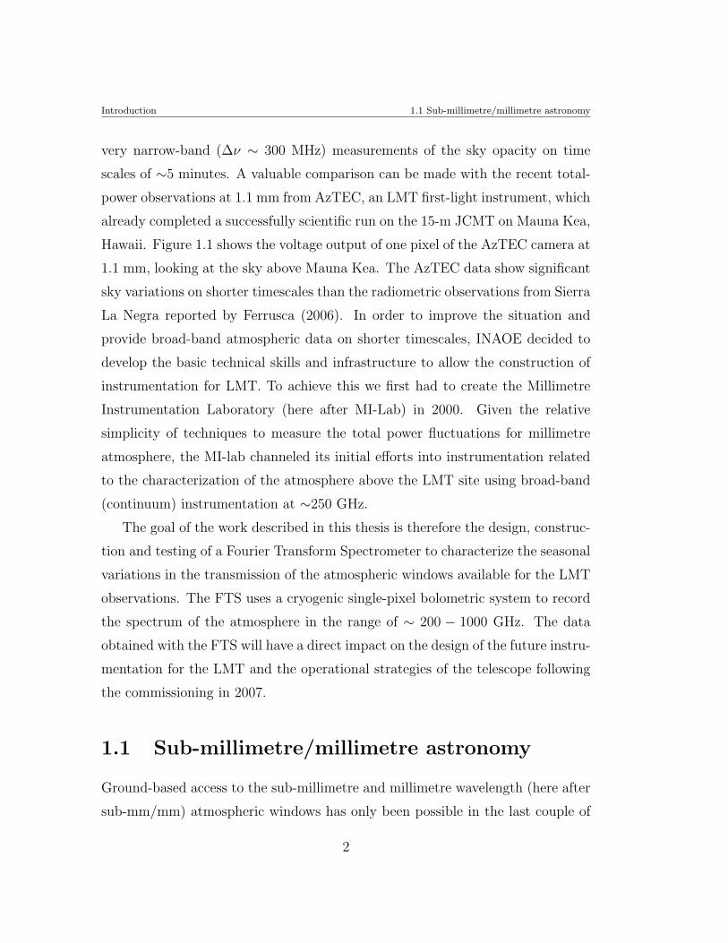
very narrow-band (∆ν ∼ 300 MHz) measurements of the sky opacity on time
scales of ∼5 minutes. A valuable comparison can be made with the recent total-
power observations at 1.1 mm from AzTEC, an LMT first-light instrument, which
already completed a successfully scientific run on the 15-m JCMT on Mauna Kea,
Hawaii. Figure 1.1 shows the voltage output of one pixel of the AzTEC camera at
1.1 mm, looking at the sky above Mauna Kea. The AzTEC data show significant
sky variations on shorter timescales than the radiometric observations from Sierra
La Negra reported by Ferrusca (2006). In order to improve the situation and
provide broad-band atmospheric data on shorter timescales, INAOE decided to
develop the basic technical skills and infrastructure to allow the construction of
instrumentation for LMT. To achieve this we first had to create the Millimetre
Instrumentation Laboratory (here after MI-Lab) in 2000. Given the relative
simplicity of techniques to measure the total power fluctuations for millimetre
atmosphere, the MI-lab channeled its initial efforts into instrumentation related
to the characterization of the atmosphere above the LMT site using broad-band
(continuum) instrumentation at ∼250 GHz.
The goal of the work described in this thesis is therefore the design, construc-
tion and testing of a Fourier Transform Spectrometer to characterize the seasonal
variations in the transmission of the atmospheric windows available for the LMT
observations. The FTS uses a cryogenic single-pixel bolometric system to record
the spectrum of the atmosphere in the range of ∼ 200 − 1000 GHz. The data
obtained with the FTS will have a direct impact on the design of the future instru-
mentation for the LMT and the operational strategies of the telescope following
the commissioning in 2007.
1.1 Sub-millimetre/millimetre astronomy
Ground-based access to the sub-millimetre and millimetre wavelength (here after
sub-mm/mm) atmospheric windows has only been possible in the last couple of
2
Introduction 1.1 Sub-millimetre/millimetre astronomy
Figure 1.1: Voltage output of one pixel of the AzTEC camera at 1.1 mm, looking
at the sky above Mauna Kea. The top panel shows the sky variations over a
times-scale of 1 minute. The two curves show measurements taken under differ-
ent sky opacity conditions(τ215GHz ∼ 0.034, dark-line; τ215GHz ∼ 0.114, red-line).
The bottom panel shows the power-spectrum density of the sky under the opac-
ity conditions shown in the upper panel, where the dark-line and red-line again
represent low and high opacity conditions.
3

Introduction1.2 High-z Universe at sub-mm/mm
wavelengths
decades due to the improvements in telescope design and instrument technology
(e.g. large aperture telescopes and detections systems based on thermal devices).
Observational evidence shows that the Universe is full of very cold material such
as planets (with surface temperatures ∼ 40 - 750 K), comets (∼10 K at the Oort
Cloud and close to 300 K when approaching to the Solar System) and galax-
ies which contain cold neutral gas and cold molecular gas (T<20 K). All these
objects are consequently strong radiators at FIR/sub-mm/mm wavelengths, and
the properties of the dusty ISM are strongly related to early evolutionary stages
of the galaxies, stars and planets. Furthermore, since the Universe is transparent
to sub-mm/mm wavelengths, we are able to measure the rest-frame peak of the
FIR emission, which is strongly related to the stellar formation rate obscured
by dust in local galaxies and also in galaxies at the highest redshift with the
sub-mm/mm observations. In order to understand the origin and evolution of
these fundamental astronomical objects, experimental data with suitable reso-
lution ans sensitivity at sub-mm/mm wavelengths are required. Therefore the
LMT will play an important role in modern astronomy and astrophysics.
1.2 High-z Universe at sub-mm/mm
wavelengths
The Universe is full of cold discrete sources and a diffuse background that radi-
ate strongly at FIR - sub-mm/mm wavelengths. Six decades ago the Big-Bang
model, was proposed as an explanation for the origin of the Universe. The Big-
Bang model predicts an expanding Universe that causes a redshift in the light
coming from very distant objects, which is proportional to their distance from
the observer. Also, the model predicts the existence of the isotropic Cosmic Mi-
crowave Background (here after CMB) radiation that fills the entire Universe. In
1964, Penzias & Wilson were the first to detect a signal with the expected char-
4
Introduction1.2 High-z Universe at sub-mm/mm
wavelengths
acteristics of the CMB (Alpher et al., 1948). They measured an excess isotropic
sky signal at 4 MHz, using their 20-foot horn reflector antenna in Holmdel, New
Jersey, and were not able to attribute the signal to terrestrial sources or any kind
of noise coming from their equipment. The signal was equivalent to a blackbody
emitter with a temperature of 3.5 ± 1 K, originating from primordial radiation
at an epoch when the Universe was very hot and dense (Penzias & Wilson, 1965;
Dicke et al., 1965), and the radiation and the matter were strongly coupled. As
the Universe cooled to T ∼ 10000 K, photons no longer interacted efficiently with
the matter and they started to travel freely. In this radiation-dominated epoch,
the Universe was in thermodynamic equilibrium and hence produced a Planckian
energy distribution which has not been affected by continuous the expansion of
the Universe.
The CMB is one of the most exciting topics in modern cosmology and astron-
omy. After the first detection of the CMB, many other experiments have been
designed in order to measure the CMB power spectrum on different angular scales
which provides information on cosmological parameters and the amplitude of the
initial acoustic oscillation in baryon-photon fluid, etc. Three different types of ex-
periments have conducted CMB observations: (i) Satellites, e.g. COBE, WMAP;
(ii) Balloon-borne, e.g. BOOMEranG, MAXIMA, ARCHEOPS, QMAP; (iii)
Ground-based, e.g. CAT, TOCO/MAT, Viper, ACBAR, DASI, CBI, Saskatoon,
Tenerife.
In 1989 the Cosmic Background Experiment satellite (COBE) confirmed with
FIRAS (Far Infrared Absolute Spectrophotometer experiment) that the distri-
bution of energy of CMB was isotropic and fitted a blackbody curve described
with a temperature of 2.725±0.0002 K, (Mather et al., 1990). The Differential
Microwave Radiometer (3-10 mm, DMR) experiment on COBE also discovered
a small signal of 30 µK fluctuations (∼10 deg), (Bennett et al., 1996). This
anisotropy is evidence of variations in density which would eventually evolve into
galaxies, clusters and other larges structures. Finally, DIRBE (Diffuse Infrared
5
Introduction1.2 High-z Universe at sub-mm/mm
wavelengths
Background Experiment) mapped the entire sky at FIR wavelengths to extend
the previous observations of the infrared Astronomy Satellite IRAS (1983). The
Wilkinson Microwave Anisotropy Probe (WMAP) satellite was launched in 2001,
with the mission to observe, with a resolution of ∼0.3 deg, and sensitivity of 20
µK per 0.3 square deg the CMB which showed temperature differences of ∼ 10−6
K (see Figure1.2).
Other evidence to support the suggestion of a cold and active Universe was
provided by the IRAS satellite, which conducted an all sky FIR survey in 1983.
Imaging the sky at 12, 25, 60, 100 µm (2 arcmin FWHM), IRAS detected
∼350,000 individual point sources, of which 75% were galaxies at low redshift
z∼0.02 (Soifer et al., 1987). Whilst the majority were identified as late type
spirals, IRAS also discovered a new population of luminous infrared starburst
galaxies (LIRG’s) with a monochromatic (60 µm) luminosities LFIR > 1012L.
The combined FIR emission of these objects is larger than the total luminosity
in all others bands, (Sanders & Mirabel, 1996). The energy distribution and lu-
minosity is due to dust in the interstellar medium heated to 30 - 80 K by the
optical-UV photons (i.e. attributed to the primary radiation from young massive
stars forming at rates of >100 M/yr) and re-radiated into FIR region. IRAS
confirmed the existence of the cosmic infrared background CIB (i.e. unresolved
high-z objects). The CIB has a total energy density ∼ 40× 10−9 W/m2/sr, com-
pared with the optical background (17±3)×10−9 W/m2/sr (Franceschini, 2001),
where 30% of the CIB energy density belongs to the local universe. The rest of
this energy density could be attributed to a large population of isothermal objects
distributed over a range of redshifts (z>1) with similar SED to those local objects
called ultraluminous infrared galaxies (ULIRG’s). A more precise measurement
of the CIB was made by COBE/DIRBE (42 arcmin FWHM) which discovered
that the CIB is isotropic. The IRAS survey was also used to determine the 60
µm galaxy luminosity function, (Saunders et al., 1990), which helps to constrain
the evolution models of the starburst galaxy population in order to understand
6
Introduction1.2 High-z Universe at sub-mm/mm
wavelengths
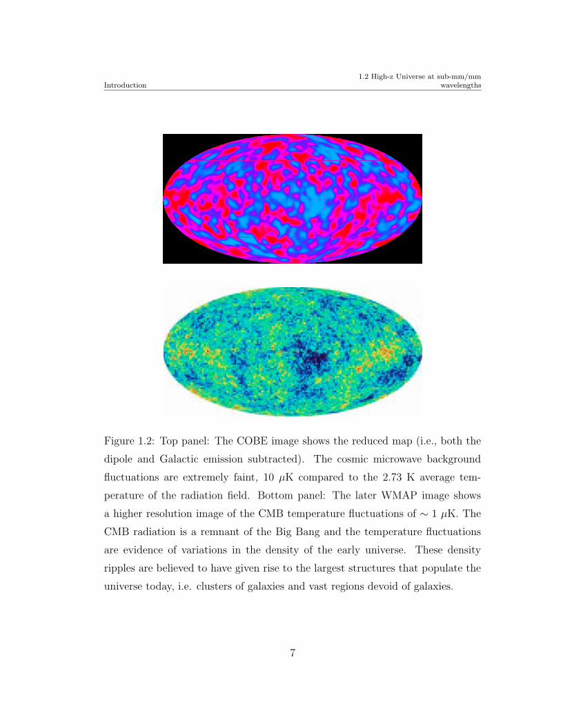
Figure 1.2: Top panel: The COBE image shows the reduced map (i.e., both the
dipole and Galactic emission subtracted). The cosmic microwave background
fluctuations are extremely faint, 10 µK compared to the 2.73 K average tem-
perature of the radiation field. Bottom panel: The later WMAP image shows
a higher resolution image of the CMB temperature fluctuations of ∼ 1 µK. The
CMB radiation is a remnant of the Big Bang and the temperature fluctuations
are evidence of variations in the density of the early universe. These density
ripples are believed to have given rise to the largest structures that populate the
universe today, i.e. clusters of galaxies and vast regions devoid of galaxies.
7
Introduction1.2 High-z Universe at sub-mm/mm
wavelengths
the spectral composition of the CIB.
Higher angular resolution studies were not made until the Infrared Space
Observatory was launched in 1995. The three-year mission provided evidence
that further supported a population of optically-obscured sources at high-z. The
ISOPHOT (a 170 µm photometer) deep extragalactic survey (Far Infrared Back-
ground project, FIRBACK) detected sources as faint as ∼100 mJy, which con-
tribute ∼10% (z< 2) of the CIB (Puget et al., 1999). Therefore, an important
result of the confirmation of the CIB is the fact that most of the star formation is
produced in a heavily-obscured interstellar medium. Furthermore, due to a strong
k-correction, sub-mm/mm wavelength observations are even more capable of pro-
viding information to trace the star formation evolution in dusty galaxies in the
high-z Universe, (Hughes & Dunlop, 1999). For example, if a large population of
ULIRG’s (e.g. Arp 220, L60 = 8.4×10¹¹L) are at z> 1 then the strong negative
k-correction at sub-mm/mm wavelengths will make their detection possible out
to redshifts as high as z∼10 (Blain et al. 2002, see Figure 1.3). The sub-mm/mm
emission of local ULIRG’s is also due mainly to dust, and it is well described by
optically-thin thermal emission greybody with temperatures between 20 to 80 K.
The greybody spectrum is due to the shape, size and composition of dust grains
(i.e. small grains are unable to emit efficiently at wavelengths similar to or larger
than their sizes, i.e. λ ≥ 2πa).
Therefore, the rapid increase in our understanding of the high-z redshift Uni-
verse and the technological development of telescopes and receivers, operating
at FIR-mm wavelengths, over the last few decades, the capability to detect of
sub-mm/mm radiation from distant galaxies is one of the most important and re-
cent developments in observational cosmology. The most successful sub-mm/mm
extragalactic surveys have been conducted since 1997 with the Submillimetre
Common -User Bolometer Array (SCUBA) on the 15-m James Clerk Maxwell
Telescope (JCMT) on Mauna Kea, Hawaii. The SCUBA galaxy source-counts
have been used to constrain the evolutionary history of dust-enshrouded star-
8
Introduction1.2 High-z Universe at sub-mm/mm
wavelengths
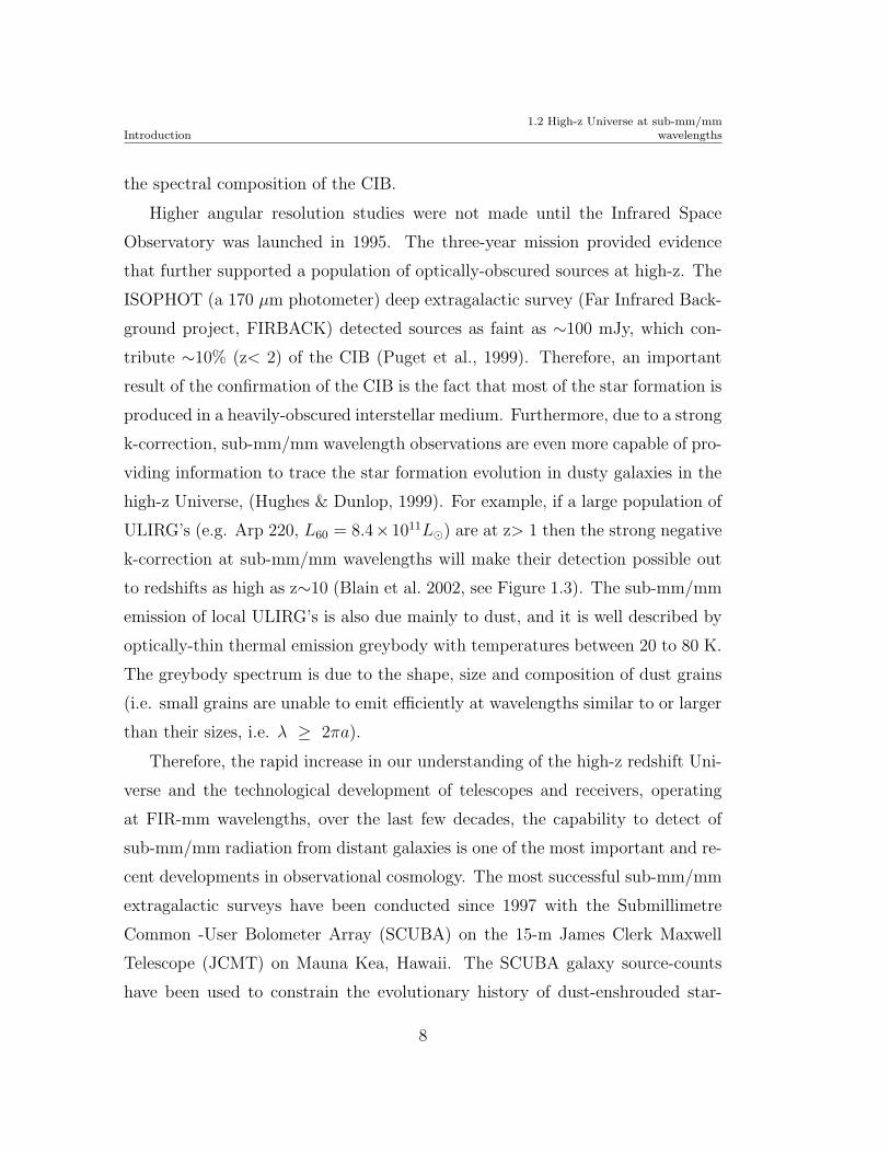
Figure 1.3: Flux density of a ULIRG (e.g. Arp 220) as a function of the redshift.
The flux density is observed at wavelengths of 175, 450 and 850 µm, over a range
of redshifts z = 0.1−10. The lines of different thickness illustrate 20 K, 40 K and
80 K SED temperatures. The graphs were made using a pure evolution model
(i.e. 5 × 10¹², β = 1.5, Ωo = 0.3 and ΩΛ = 0.7). As the SED is redshifted, it
becomes fainter, but the negative k-correction compensates for this dimming, and
so the flux remains basically constant for z ∼ 1− 8 (e.g. at 850 µm wavelength).
In the case of longer wavelengths or warmer SEDs, the k-correction increases the
observed flux at higher redshifts.
9
Introduction1.2 High-z Universe at sub-mm/mm
wavelengths
burst galaxies at z ∼2 - 3, as well as the intensity of the background radiation
at sub-mm/mm wavelengths (Smail et al., 1997; Hughes et al., 1998; Scott et al.,
2002).
However, todate less than 1 sq. degree of the entire sky has been mapped
at sub-mm/mm wavelengths, because the actual surveys are still restricted by
the angular resolution, sensitivity and field-of-view. For example, SCUBA and
MAMBO on the 30-m IRAM telescope, have mapped individual regions with ar-
eas of 0.002 - 0.2 sq degree and have resolved close to 20% of the total radiation
at FIR wavelengths measured by COBE/DIRBE. A new generation of large for-
mat array cameras (SCUBA-II; ∼ 64000 pixeles) will allow one to significantly
improve the mapping speed by fully-sampling the focal plane of the 15-m JCMT
telescope in the near future. On the other hand, the small primary apertures
of these existing sub-mm telescopes, limit the sensitivities of the source detec-
tions to an extra-galactic confusion limit of ∼2 mJy at 850 µm, with 15 arcsec
resolution. A larger single-dish millimetre wavelength telescope will provide a
greater gain in both sensitivity and resolution and, combined with large format-
array cameras, will significally increase the mapping speeds. Therefore the 50-m
LMT millimetre-wavelength observations will be extremely important in tracing
the evolution of the star formation in dusty enviroments at high-z. For exam-
ple AzTEC (Aztronomical Thermal Emission Camera) is one of the first-light
instruments for the LMT. AzTEC uses a 144-pixel SiNi spider-web bolometer
array operating at 1.1 and 2.1 mm, with a FOV of 2.4 sq. arcmin. Given the
predicted AzTEC sensitivity (NEFD ∼ 3 mJy−1/2 per pixel at 1.1 mm), and a
mapping-speed of ∼ 0.3 deg2hr−1mJy−2 on the LMT, as well increasing the high
angular resolution, AzTEC and the LMT will reduce the measured extragalac-
tic confusion limits. This will make it possible to resolve a significant increased
fraction (90 - 100%) of the mm-FIR wavelength background into individual point
sources (i.e. LFIR > 1011L). In addition, the large-scale structure of the Uni-
verse will be studied with the LMT by conducting observations of clusters via the
10
Introduction1.2 High-z Universe at sub-mm/mm
wavelengths
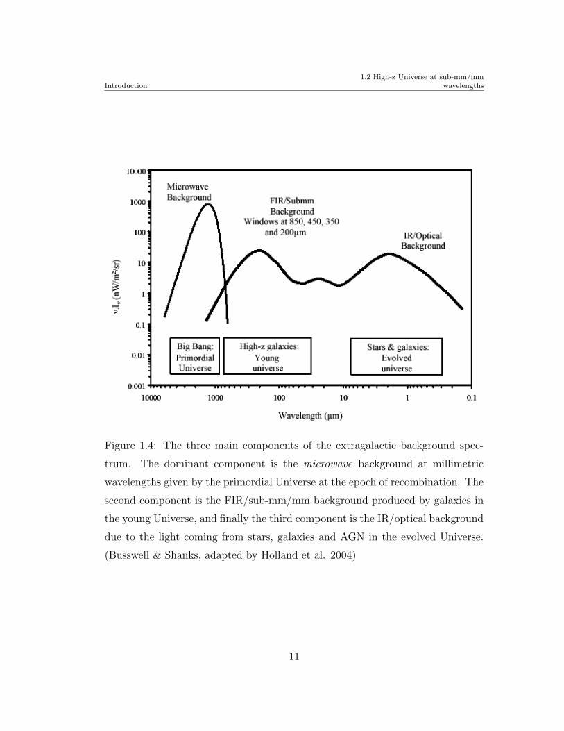
Figure 1.4: The three main components of the extragalactic background spec-
trum. The dominant component is the microwave background at millimetric
wavelengths given by the primordial Universe at the epoch of recombination. The
second component is the FIR/sub-mm/mm background produced by galaxies in
the young Universe, and finally the third component is the IR/optical background
due to the light coming from stars, galaxies and AGN in the evolved Universe.
(Busswell & Shanks, adapted by Holland et al. 2004)
11
Introduction 1.3 Ground-based observations at sub-mm/mm
Sunyaev-Zeldovich effect, with AzTEC observing at both 1.1 mm and 2.1 mm the
increment and decrement of the S-Z signature, (Hughes, 2005). Therfore, hav-
ing motivated and justified the many opportunities to conduct exciting scientific
projects at FIR-millimetric wavelengths, in particular with the LMT, we now
describe the unavoidable impact of the atmosphere on ground-based millimetric
wavelengths observations.
1.3 Ground-based observations at sub-mm/mm
Despite the growing importance of the sub-mm/mm astronomy in understand-
ing the evolution and growth of the structure in the Universe, it is currently
only practical to make the majority of these observations from ground-based ob-
servatories. At sub-mm/mm (∼ 4 mm - 300 µm), the atmosphere is partially
transparent. In this region there is absorption and emission from a variety of
molecules (CO, NH3, HCl, etc ...). There are windows of excellent transmission
between ∼50 GHz and 300 GHz, but these still include some features from H2O
and O2. With the exception of two wide windows at 650 GHz and 850 GHz,
however, the atmosphere is completely opaque at higher frequencies until one
reaches the mid infrared (∼10 THz). This high atmospheric opacity is due to wa-
ter molecules and dioxide of carbon and ozone. In addition, a pseudo-continuum
with both wet and dry components contributes to the atmospheric absorption.
This pseudo-continuum is stronger at higher sub-mm frequencies.
The atmospheric transparency is one of the most important features when
choosing a telescope site. The atmospheric opacity produces a reduction in sig-
nal strength by the absorption, and therefore longer integration times are required
to reach the desired signal-to-noise ratio. Also the atmospheric stability will pro-
duce phase delays on the incoming signal. This is produced by the non-uniform
distribution of the atmospheric water vapor, due to imperfect mixing. The water
vapor moves in layers creating a turbulent cells which impose a limit for interfer-
12
Introduction 1.4 The atmosphere
ometric observations. In addition, time fluctuations on the sky temperature due
to the water vapour are an important source of sky-noise for ground-based obser-
vations. Atmospheric models are helpful in conjunction with observational data
programs to study the strategies for site characterization (Surtees, 1991). Models
of the atmospheric spectrum were first presented by van Vleck (1947a,b). The
current favored model is the Atmospheric Transmission Model, (ATM) (Pardo et
al. 2001). These models depend on the physical parameters, such as barometric
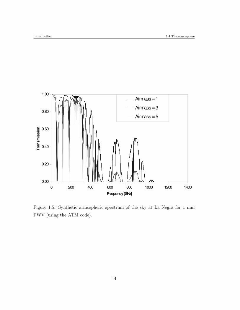
pressure or site altitude, surface temperature and amount of water (PWV) (see
Figure 1.5). In ground-based observations, beyond the issue of site-selection, it
is helpful to characterize the site before the first observations begin in order to
plan the observatory operations. Both temporal and spatial atmospheric charac-
terization are necessary and typically involve measurements of opacity, PWV and
sky stability. Previous knowledge of the sky behavior will also help in the design
of the electronic systems (control and readout) for the next generation of de-
tectors, for example those based on superconductors materials (superconducting
transition-edge sensors, TES). Therefore removing the effect of the atmospheric
water-vapour is the major challenge in ground-based sub-mm/mm observational
astronomy. One way to minimize the water-vapour problem is to build observa-
tories in high and dry sites, where atmospheric water content is small or ideally,
ignoring the financial implications, telescopes on balloon-borne or satellite plat-
forms. The next sections will describe briefly some atmospheric properties and
characteristics, and some of the methods to study the atmosphere that ultimately
motivated our decision to build a FTS system.
1.4 The atmosphere
The Earth is surrounded by gases that we call atmosphere. The atmosphere is
a mix of gases (air) formed by nitrogen (79%), oxygen (20%) and other gases
(1%). The atmosphere is dived into many layers. Strong correlations exist be-
13
Introduction 1.4 The atmosphere
0.00
0.20
0.40
0.60
0.80
1.00
0 200 400 600 800 1000 1200 1400
Frequency [GHz]
Tran
smis
sion
.
Airmass = 1
Airmass = 3
Airmass = 5
Figure 1.5: Synthetic atmospheric spectrum of the sky at La Negra for 1 mm
PWV (using the ATM code).
14
Introduction 1.5 Water vapour absorption
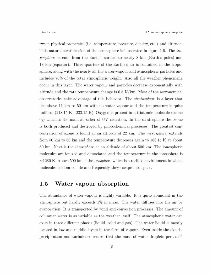
tween physical properties (i.e. temperature, pressure, density, etc.) and altitude.
This natural stratification of the atmosphere is illustrated in figure 1.6. The tro-
posphere extends from the Earth’s surface to nearly 8 km (Earth’s poles) and
18 km (equator). Three-quarters of the Earths’s air is contained in the tropo-
sphere, along with the nearly all the water-vapour and atmospheric particles and
includes 70% of the total atmospheric weight. Also all the weather phenomena
occur in this layer. The water vapour and particles decrease exponentially with
altitude and the rate temperature change is 6.5 K/km. Most of the astronomical
observatories take advantage of this behavior. The stratosphere is a layer that
lies above 11 km to 50 km with no water-vapour and the temperature is quite
uniform (218.15 K - 233.15 K). Oxygen is present in a triatomic molecule (ozone
03) which is the main absorber of UV radiation. In the stratosphere the ozone
is both produced and destroyed by photochemical processes. The greatest con-
centration of ozone is found at an altitude of 22 km. The mesosphere, extends
from 50 km to 80 km and the temperature decreases again to 183.15 K at about
80 km. Next is the ionosphere at an altitude of about 500 km. The ionospheric
molecules are ionized and dissociated and the temperature in the ionosphere is
∼1280 K. Above 500 km is the exosphere which is a rarified environment in which
molecules seldom collide and frequently they escape into space.
1.5 Water vapour absorption
The abundance of water-vapour is highly variable. It is quite abundant in the
atmosphere but hardly exceeds 1% in mass. The water diffuses into the air by
evaporation. It is transported by wind and convection processes. The amount of
columnar water is as variable as the weather itself. The atmospheric water can
exist in three different phases (liquid, solid and gas). The water liquid is mostly
located in low and middle layers in the form of vapour. Even inside the clouds,
precipitation and turbulence ensure that the mass of water droplets per cm−3
15
Introduction 1.5 Water vapour absorption
Troposphere
Stratosphere
Mesosphere
Ionosphere
Exosphere
Ozone layer
~ 8 – 18 km
~ 50 km
~ 80 km
~ 500 km
300 K273 K243 K213 K
Figure 1.6: Stratification of the Earth atmosphere showing the change in tem-
perature (K) with the increasing altitude (km).
16
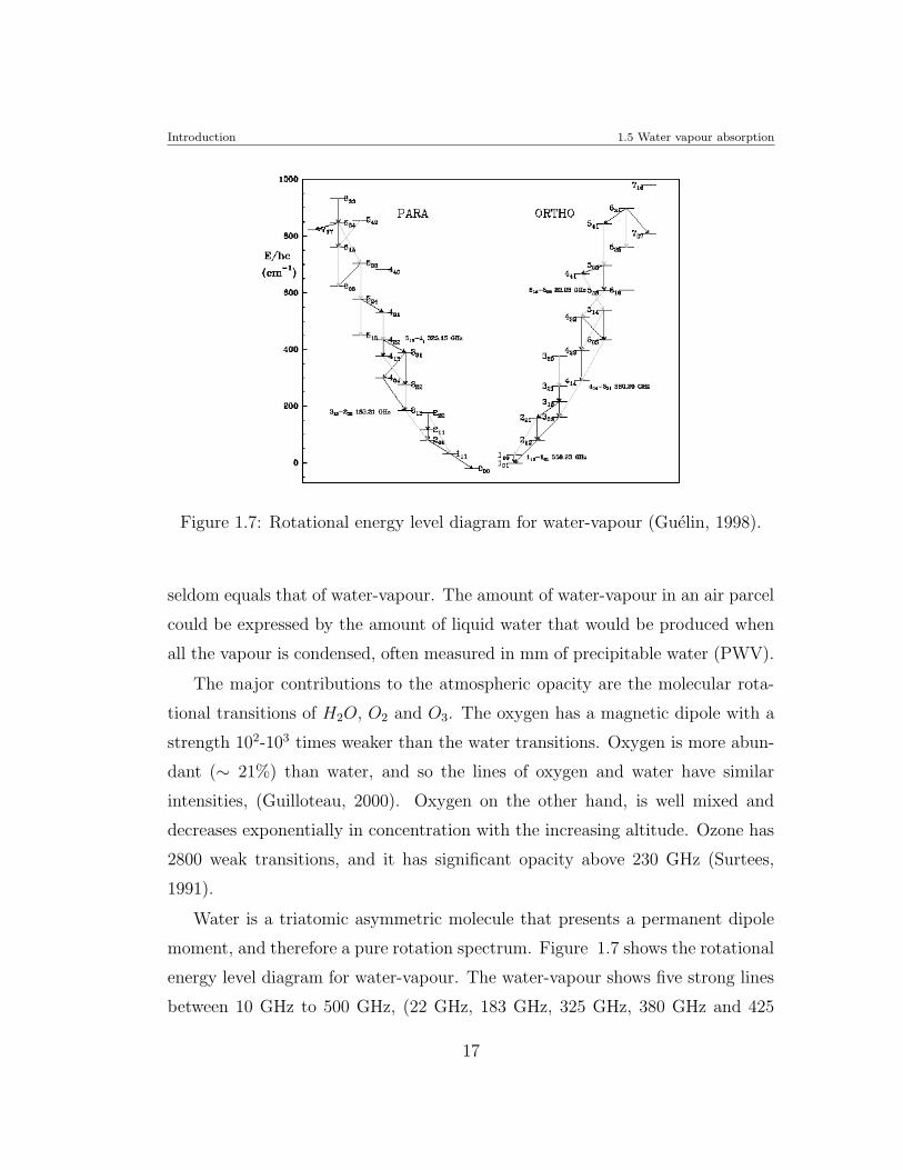
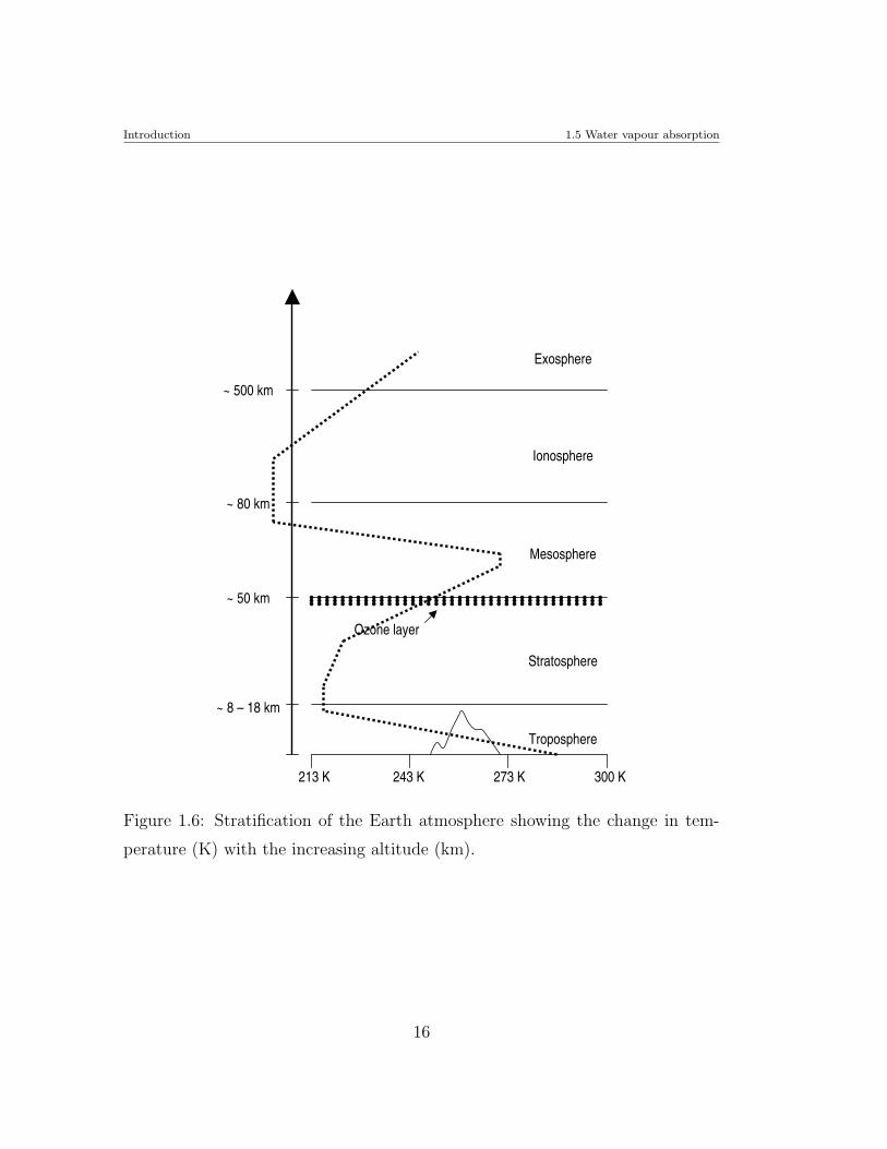
Introduction 1.5 Water vapour absorption
Figure 1.7: Rotational energy level diagram for water-vapour (Guelin, 1998).
seldom equals that of water-vapour. The amount of water-vapour in an air parcel
could be expressed by the amount of liquid water that would be produced when
all the vapour is condensed, often measured in mm of precipitable water (PWV).
The major contributions to the atmospheric opacity are the molecular rota-
tional transitions of H2O, O2 and O3. The oxygen has a magnetic dipole with a
strength 102-103 times weaker than the water transitions. Oxygen is more abun-
dant (∼ 21%) than water, and so the lines of oxygen and water have similar
intensities, (Guilloteau, 2000). Oxygen on the other hand, is well mixed and
decreases exponentially in concentration with the increasing altitude. Ozone has
2800 weak transitions, and it has significant opacity above 230 GHz (Surtees,
1991).
Water is a triatomic asymmetric molecule that presents a permanent dipole
moment, and therefore a pure rotation spectrum. Figure 1.7 shows the rotational
energy level diagram for water-vapour. The water-vapour shows five strong lines
between 10 GHz to 500 GHz, (22 GHz, 183 GHz, 325 GHz, 380 GHz and 425
17
Introduction 1.6 Measuring the atmospheric transparency
GHz). Above 500 GHz water-vapour emits strongly and produces an optically-
thick atmosphere that radiates with power > 106 times stronger than the typical
astronomical sources at sub-mm/mm wavelengths.
1.6 Measuring the atmospheric transparency
The opacity and atmospheric instability effects are important for the sub-mm/mm
wavelength range. Observations at wavelengths < 2 mm are more affected by
the atmospheric conditions and only a few sites in the world offer acceptable
conditions for sub-mm/mm astronomical observations, including the LMT site
Sierra La Negra.
1.6.1 Radiometers
Astronomical observations under high opacity conditions are futile due to the
fact that astronomical radiation can not penetrate the atmosphere. The opacity
over sub-mm/mm wavelength range is highly correlated with the amount of at-
mospheric water-vapour, so a potential site for sub-mm/mm observatory will be
a dry site at very high altitude.
A common method to measure the opacity is by means of a tipping radiome-
ter. Typically there are two types; single-line and broad-band window. Tip-
ping radiometers directly measure the total atmospheric opacity (adding all the
contributions from all the atmospheric components) at wavelengths close to the
wavelengths of the bandpasses in which the observations are being made. The at-
mospheric opacity is measured by using a tipping mirror in order to measure the
sky temperature at different elevations (e.g. 215 GHz INAOE radiometer, Tor-
res et al. 1997; Estrada et al. 2002), and a linear relation between the measured
power as function of the airmass is then fitted to these data. Currently 200-225
GHz tipping radiometers are standard for site characterization at sub-mm/mm
18
Introduction 1.6 Measuring the atmospheric transparency
wavelengths. A single-line radiometer measures the total power in a single-line,
for example at 22 GHz or 183 GHz which lie within the frequency range of strong
water emission lines. The opacity is then obtained from the amount of water by
means of atmospheric models, describing the water line-profile (Delgado et. al.,
1999).
Tipping radiometers are relatively simple to construct and operate (i.e. no
strict support is required), and they are suitable for long-term monitoring cam-
paigns. The disadvantage is that they only measure the opacity at a single wave-
length or in a broad-band window. More detailed atmospheric information over
a wide-band (e.g. ∼ 200 GHz - 2 THz) can be performed by spectroscopic meth-
ods. Wide-band radiometers are more complex and they usually require cryo-
genic cooling, as well as a more elaborate optical system. Alternatively Fourier
Transform Spectrometers (FTS) covering all the sub-mm/mm range, offering de-
tailed atmospheric spectra of the site, and have been extensively used in South
Pole (Chamberlin et al., 2003), and Pampa La Bola, Chile, for example (Matsuo
et al., 1998; Matsushita et al., 1999, 2000).
19
Introduction 1.6 Measuring the atmospheric transparency
1.6.2 Interferometers
In the sub-mm/mm wavelength range, temporal variations in the amount of at-
mospheric water-vapour cause sky instability. Because the astronomical radiation
travels more slowly through cells of water-vapour than through the dry air, fluc-
tuations in the water-vapour content will produce variations in the phase of the
detected astronomical radiation. The main consequences of these fluctuations
are: (i) loss of resolution and (ii) attenuation of the intensity of the astronomical
radiation.
Interferometers are useful to simultaneously measure the sky stability (phase/
brightness fluctuations), as well as atmospheric opacity. Whilst atmospheric sta-
bility is not as fundamental as transparency for a site characterization, it is im-
portant for observations of the faintest point sources and the extended cosmic
microwave background. Experiments to measure the anisotropy of the CMB
at small angular scales (< arcmin) are the most affected by these fluctuations.
For sub-mm/mm interferometry, the instability causes phase fluctuations and
also produces lower resolution observations. Measuring the phase fluctuations
directly with an interferometer, by observing a convenient beacon outside the
atmosphere, i.e., on a geostationary satellite, can correct the phase (Ishiguro
et al., 1990). Inhomogeneities in the atmospheric water-vapour distribution also
produce fluctuations in the sky brightness that have been measured by interferom-
eters, (Lay & Halverson, 2000). Differential measurements are usually employed
to minimize the effects of the sky instability: (i) chopped-beam instruments mea-
sure the difference in emission between two or more directions on the sky, e.g.
Python I-IV: (Dragovan et al., 1994; Ruhl et al., 1995; Platt et al., 1997; Kovac
et al., 1997), (ii) swept-beam instruments sweep a beam rapidly backward and
forward ∼5 Hz, e.g. Python V: (Coble et al., 1999); Mobile Anisotropy Exper-
iment: (Torbet et al., 1999). Both techniques efficiently reduce the noise from
rapid sky-fluctuations. A similar chopping (sky-subtracting) strategy is also used
20
Introduction 1.6 Measuring the atmospheric transparency
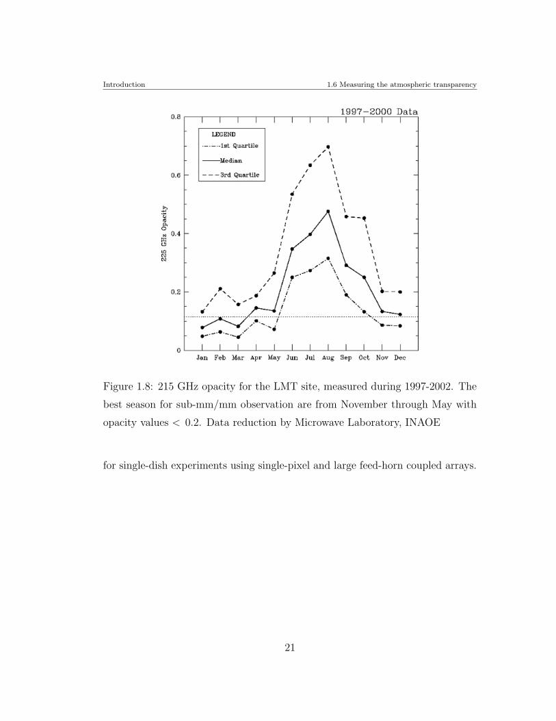
Figure 1.8: 215 GHz opacity for the LMT site, measured during 1997-2002. The
best season for sub-mm/mm observation are from November through May with
opacity values < 0.2. Data reduction by Microwave Laboratory, INAOE
for single-dish experiments using single-pixel and large feed-horn coupled arrays.
21
Introduction 1.7 LMT site characterization with a FTS
1.7 LMT site characterization with a FTS
Since 1999, there has been construction on Sierra La Negra to build a single-dish
large-aperture sub-mm/mm telescope (∼ 50 m) at an altitude of 4600 m. The
opacity of the site has been measured with water-vapour tipping radiometers at
215 GHz during 1997 - 2005 (Torres et al., 1997; Estrada et al., 2002). Sierra
La Negra is a sub-mm/mm site during a large fraction of the year (November
through May) when the opacity τ215GHz is around 0.2 or less (third quartile,
see Figure 1.8). However, the characterization of the atmospheric transparency
and stability of the LMT site has only been made with narrow-band radiometric
methods at 215 GHz (Torres et al., 1997; Estrada et al., 2002). This information
just reflects the narrow-band behavior of the sky, and a better understanding
of the atmospheric behavior is needed in order to understand the broad-band
characteristics since continuum detectors are commonly used at sub-mm/mm
wavelengths (i.e bolometers array, AzTEC, SPEED). The operational band of
a bolometric camera is defined by the available atmospheric windows (e.g. 2.1
mm, 1.1 mm, 850µm: see Figure 1.5), and the optical filtering within the camera.
In practice, however the optical bandpass filters are designed to closely match
the atmospheric windows. This maximizes the sensitivity whilst minimizing the
impact of a variable sky emission.
Also, the sky stability has a strong influence on the design of the readout
electronics, because the change in the optical background can produce changes in
sensitivity and overloading on the detector system. It is not only the broadband
systems that need atmospheric information, but also the heterodyne systems (i.e.
SEQUOIA, Z-machine, etc) which will work over a wide range of frequencies,
70 − 115 GHz, and hence are also affected by the sky conditions. Figure 1.9
illustrates the atmospheric modeled transmission from Sierra La Negra over a
range of 50 − 400 GHz showing the atmospheric behavior for summer and win-
ter seasons. The atmospheric transmission was calculated from measurements of
22
Introduction 1.7 LMT site characterization with a FTS
3 2.1 1.4 1.1 .85
λ [mm]
50 100 150 200 250 300 350 4000
0.2
0.4
0.6
0.8
1
ν [GHz]
Transmission
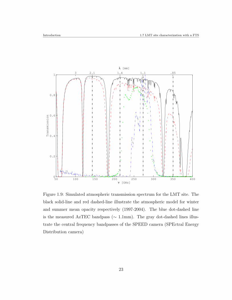
Figure 1.9: Simulated atmospheric transmission spectrum for the LMT site. The
black solid-line and red dashed-line illustrate the atmospheric model for winter
and summer mean opacity respectively (1997-2004). The blue dot-dashed line
is the measured AzTEC bandpass (∼ 1.1mm). The gray dot-dashed lines illus-
trate the central frequency bandpasses of the SPEED camera (SPEctral Energy
Distribution camera)
23
Introduction 1.8 Millimetre Instrumentation Laboratory
the mean opacity, base temperature and local pressure for the respective season.
Also, shown in figure 1.9 are the transmission characteristic of the AzTEC filter
at 1.1 mm, which is not contaminated with any water-emission lines (that occur
at 183 and 325 GHz, which define the wider sub-mm/mm window). Extensive
broad-band observations of the atmospheric transmission above the LMT site,
derived by the FTS system described in this thesis, can guide the future instru-
ments developments for the LMT. Also, the FTS system will provide information
about the percentage time of open atmospheric windows and the guidelines for
the design of the broad-band filtering, allowing us to optimize the observation
operations throughout the year. Therefore, an FTS system developed at INAOE
will be a powerful complementary instrument for a continuous site characteriza-
tion program. Furthermore by optimizing the design of the first instruments, the
LMT will play a leading-role in the coming decades in the investigations into the
formation and evolution of the structure at all epochs.
1.8 Millimetre Instrumentation Laboratory
The MI-Lab was created to design and build instruments for the site characteriza-
tion, scientific experiments, as well as to provide support to the LMT instruments
by forming the necessary human resources through the technical training of stu-
dents. In order to design, build and integrate the cryogenic FTS system as part
of this development, we first had to establish the suitable working space for a
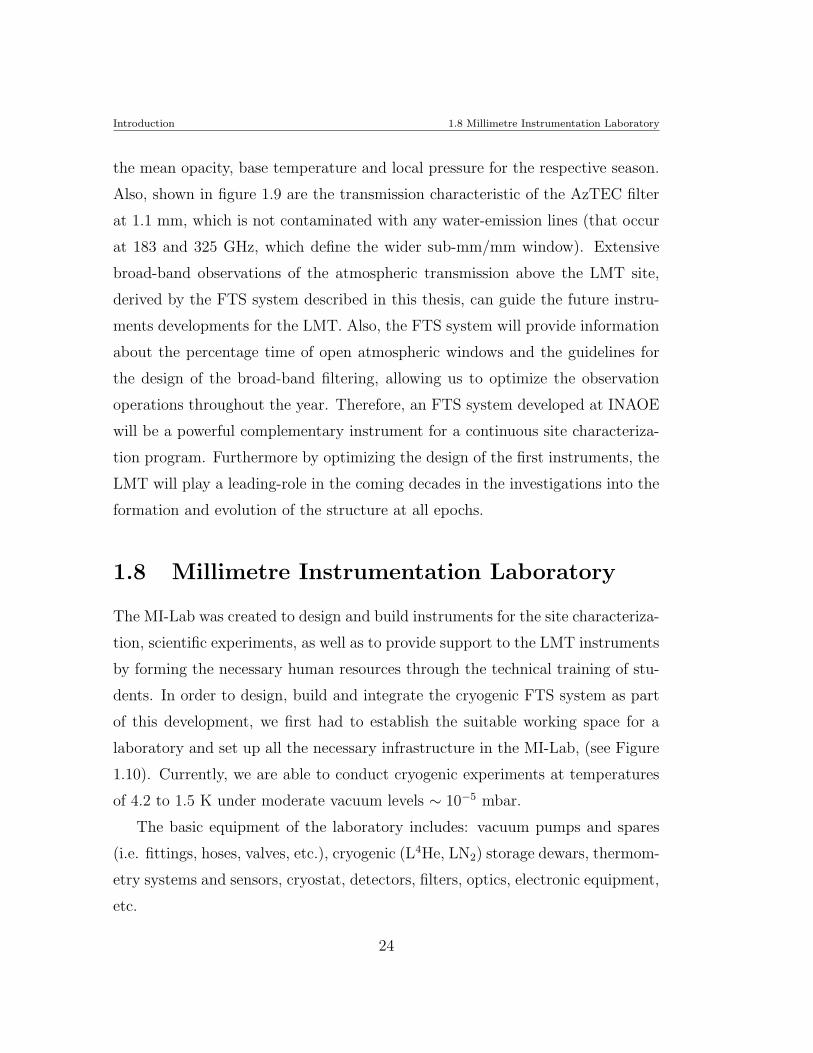
laboratory and set up all the necessary infrastructure in the MI-Lab, (see Figure
1.10). Currently, we are able to conduct cryogenic experiments at temperatures
of 4.2 to 1.5 K under moderate vacuum levels ∼ 10−5 mbar.
The basic equipment of the laboratory includes: vacuum pumps and spares
(i.e. fittings, hoses, valves, etc.), cryogenic (L4He, LN2) storage dewars, thermom-
etry systems and sensors, cryostat, detectors, filters, optics, electronic equipment,
etc.
24
Introduction 1.8 Millimetre Instrumentation Laboratory
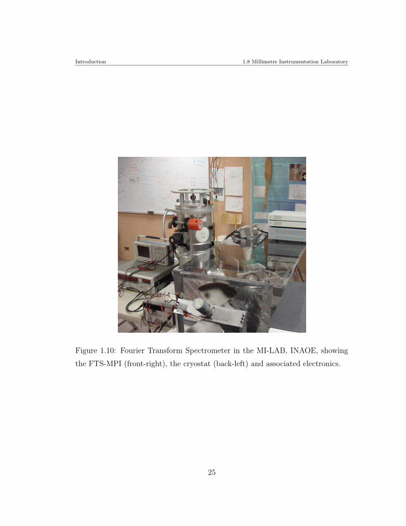
Figure 1.10: Fourier Transform Spectrometer in the MI-LAB, INAOE, showing
the FTS-MPI (front-right), the cryostat (back-left) and associated electronics.
25
Introduction 1.9 Objective of the thesis
1.9 Objective of the thesis
At the start of this effort to build and develop experience in sub-mm/mm wave-
length instrumentation at INAOE, we asked a few straight-forward questions. Is
it possible to characterize the atmospheric conditions of the sky for LMT site
in the sub-mm/mm range by building at INAOE a cryogenic Fourier Transform
Spectrometer, instead of buying a commercial one? Is a Fourier Transform spec-
trometer a suitable instrument for the purpose of characterizing the atmosphere
above Sierra La Negra? It is possible to use a cryogenic composite bolometer
operating temperatures above 1 K in order to make measurements over the sub-
mm/mm range? In order to answer the above questions, we proposed to design
and construct a Fourier transform spectrometer using a single-pixel cryogenic
camera, based on a composite bolometer operating at temperatures < 2 K. The
composite bolometer uses a NTD Ge thermistor type-B from Haller-Beeman Inc.
and uses NbTi electrical leads which would allow us to measure radiation levels
as low as 10−12 W. The advantage of the NbTi wires is that they reduce the
thermal conductance by a factor ∼100 compared to brass, and by a factor of
∼1000 compared to copper at cryogenic temperatures as low as 1.8 K. The final
working temperature of the system is ∼ 1.8 K (under vacuum), which provides
an expected thermal conductance close to 1 × 10⁻¹⁰ W/K, allowing the system
to work with backgrounds of about 10−12 W. The responsivity of the detection
system is 3 × 10⁶ V/W and the NEP is 1.26 × 10⁻¹³ W/Hz1/2. In order to have
a compact system we decided to adopt a medium-throughput system (i.e. ∼ 8.9
cm, ∼ f/4.7) and a small linear stage (i.e. 18 cm) without sacrificing the spectral
resolution. The FTS-MPI system allows us to measure a broad-band spectrum
in the 215 - 1000 GHz frequency range with a resolution from 10 GHz - 500 MHz.
As an important secondary goal, the FTS could provide detailed (high-resolution)
measured atmospheric spectra for comparison with models (e.g. ATM), and al-
low us to set up a continuous program of site characterization and monitoring
26
Introduction 1.10 Thesis Outline
with the following objectives: (i) to identify and quantify the site conditions and
their influence on the design and operation of the current, as well as the future
instruments; (ii) to provided historical records of the site conditions to guide the
efficient future operation of the LMT observatory (i.e flexible queue scheduling,
engineering maintenance periods, etc.).
The present work also deals with the development of a methodology for the
design and integration skills, that will lead to the development of future sub-
mm/mm astronomical instrumentation at INAOE in Mexico.
One important factor is the experimental quantification of the thermal prop-
erties of the NbTi wires, which were expected to have a suitable behavior for
operational temperatures lower than 2 K, but for which insufficient data existed
in the literature prior to this decision. Finally we developed a complete Fourier
transform spectrometer that operates at sub-mm/mm wavelengths, that includes
the optics which were completely fabricated at the INAOE facilities.
1.10 Thesis Outline
The design of FTS-MPI system is described in this thesis, which is part of the
first instrumentation projects conducted by the MI-Lab at INAOE. The basic
Fourier transform spectroscopy, based on a polarizing Martin-Puplett interfer-
ometer, is reviewed in Chapter 2, as well as a brief discussion about using a
bolometric camera as part of the FTS-MPI. The detection system is based on
cryogenic bolometer, and the basic theory is reviewed in Chapter 3. The design
of the bolometer, optical coupling, cryogenic system, readout electronics and the
performance analysis is developed in the Chapter 4. The design of the FTS-MPI,
as well as the integration of the system is described in Chapter 5, and in addi-
tion we discuss the data reduction method and first results from the laboratory
tests. In Chapter 6, the final conclusions and the summary of the result of this
project are presented. A discussion of the modifications to the system in order
27

Introduction 1.10 Thesis Outline
to provided an operational spectroscopic instrument, installed at the LMT are,
also presented as part of the future work.
28
Chapter 2
Fourier Transform Spectrometry:
FTS
This chapter deals with the theory of Fourier transform spectroscopy, and the
Fourier transform method of interference spectroscopy via which a spectrum can
be recorded and analyzed. The basic properties i.e apodization, interferogram
sampling and spectrum computation are discussed in order to understand the
performance of the Fourier spectrometer. The spectroscopic process can be di-
vided into two main parts: the first, the recording of the interferogram; and the
second, the computation of the spectrum from the Fourier-transform of the in-
terferogram. The discussion is then extended to the design of our FTS system
at INAOE, based on the Martin-Puplett interferometer which is widely used for
far-infrared experiments and astronomy studies.
29
Fourier Transform Spectrometry: FTS 2.1 Interference Spectroscopy
2.1 Interference Spectroscopy
A spectrometer is an instrument that separates the continuous radiation from the
electromagnetic spectrum into individual higher resolution measurements (spec-
tra). There exist several types of spectrometers, each used in different research
fields. Generally a spectrometer works over a small fraction of frequencies in the
electromagnetic spectrum. The spectrometers are mainly divided in two cate-
gories: (i) Dispersing spectrometers (e.g. prism spectrometer, diffraction spec-
trometer); (ii) interference spectrometers (e.g. two-beam interferometer, multi-
beam interferometer).
The dispersing interferometers or diffraction gratings, spatially separate the
individual frequency components (monochromators) of the incoming radiation.
Each frequency component is selected by a slit and measured with a suitable
detector. The final spectrum is obtained after measuring all the frequency com-
ponents of interest. The main drawback is their slow scanning process when
used as a monochromator. In comparison the interferometric method uses an
interferometer which divides the incoming radiation into two or more paths (i.e.
multi-beam systems) and then recombines the beams after a phase delay has been
introduced into one of the beams. This delay produces an interference pattern
which is detected and recorded. The recombined signal is called an interferogram,
which is the Fourier Transform of the power spectrum of the incoming radiation.
Therefore, the inverse Fourier Transform of the interferogram will yield the origi-
nal power spectrum. The main drawback in Fourier transform spectroscopy comes
from the post-observation mathematical process which can introduce errors into
the final computed spectrum. Methods to reduce the impact of these errors are
discussed.
30
Fourier Transform Spectrometry: FTS 2.1 Interference Spectroscopy
2.1.1 Two beam interference
Mathematically the interference could be explained as simply the superposition
of two scalar waves. The nature of the light is vectorial (electric and magnetic
fields are both vectorial). The electric field E at any point in space could be
represented by the combined fields E1,E1,..., from different sources,
E = E1 + E2 + · · · (2.1)
Since the electric field varies too fast, a better quantity to measure by a variety
of detectors such as the bolometers, is the radiant flux density S. The radiant
flux density is defined as,
I = 〈S〉 = ευ⟨
E2⟩
(2.2)
where the term in brackets is the squared time-average magnitude of the intensity
of the electric field. Now we consider a beam of radiant energy divided into two
parts. Those two beams superpose at a point Q after travelling different paths.
Let E1(t) and E2(t) be the analytic representation of the beams. Each beam is
represented at Q as k1E1(t− θ1) and k2E2(t− θ2), where θ is the time delay and
k is a geometric factor. The superposed beams can be expressed as a vectorial
sum,
E(t) = k1E1(t − θ1) + k2E2(t − θ2), (2.3)
using the expression for the radiant flux with the Eq.(2.3) we get
I =⟨
E(t)E(t)∗⟩
,
31
Fourier Transform Spectrometry: FTS 2.1 Interference Spectroscopy
where E(t)E(t)∗ = k1k2E1(t − θ1)E∗
1(t − θ1)
+ k1k2E2(t − θ2)E∗
2(t − θ2)
+ k1k∗
2E1(t − θ1)E∗
2(t − θ2)
+ k∗
1 k2E∗
1(t − θ1)E2(t − θ2). (2.4)
The first and the second terms of Eq.(2.4) are the radiant flux densities at Q
without any interference. The third and fourth terms are the complex conjugates
of each one, such that their sum is
2 |k1k2| <
E1(t − θ1)E∗
2(t)
. (2.5)
Using Eq.(2.5), and the fact that I1(t) =⟨
E1(t)E1(t)∗
⟩
, I2(t) =⟨
E2(t)E2(t)∗
⟩
and that kk∗ = |k|2, then I(t) at Q is,
I(t) = |k1|2 I1(t) + |k2|2 I2(t) + 2 |k1k2| <⟨
E1(t − θ1)E∗
2(t)⟩
(2.6)
2.1.2 Frequency information
The frequency information is contained in the interference pattern. The quantity
< E1(t − θ1)E∗
2(t) > in the third term of Eq. 2.6 is the mutual coherence of
the two beams. This term is a cross-correlation function from which we obtain
the cross-power spectrum by taking the Fourier transform. We can express the
mutual coherence as,
C12(θ) = Γ12(θ) (2.7)
If the two beams came from the same source in such way that E1(t) = E2(t) we
get the auto-correlation function of the source. Therefore the Fourier transform
gives the power density spectrum denoted by B(ν):
B(ν) =
∫ +∞
−∞
C11(θ)exp(−2πiνθ)dθ (2.8)
32
Fourier Transform Spectrometry: FTS 2.1 Interference Spectroscopy
Using the inversion theorem,
C11(θ) =
∫ +∞
−∞
B(ν)exp(2πiνθ)dν (2.9)
Realizing the following substitutions to put these equations (2.8,2.9) in terms of
the path difference and wavenumber,
θ = δ/c,
ν = σc,
C11(θ) = I(δ),
B(ν) = I(σ).
we obtain expressions
I(δ) =
∫ +∞
−∞
I(σ)exp(2πiσδ)dσ (2.10)
I(σ) =
∫ +∞
−∞
I(δ)exp(−2πiσδ)dδ (2.11)
The expression in Eq. (2.10) is the auto-correlation of the source, and it is a
function of the path difference δ. Therefore, recording the interferogram and
taking the Fourier transform, we can obtain a computed source spectrum.
2.1.3 The finite retardation and apodization
The computed spectrum is not a perfect representation of the true spectrum, since
the interferogram is not measured over an infinitely long path-difference, and
hence the result is a truncated interferogram. Mathematically this truncation
can be expressed as the result of the complete interferogram multiplied by a
truncation function D(δ) defined as,
D(δ) = 1 |δ| < L
= 0 |δ| ≥ L,(2.12)
33
Fourier Transform Spectrometry: FTS 2.1 Interference Spectroscopy
where L is the maximum retardation. The product of two functions, say D(δ)
and I(δ), is the convolution of the Fourier transform of each function. Conse-
quently, the computed spectrum is the true spectrum convolved with the Fourier
Transform of the truncation function. The Fourier Transform of D(δ) is the sinc
function:
F [D(δ)] = 2Lsin(2πσL)
2πσL= 2Lsinc(2πσL). (2.13)
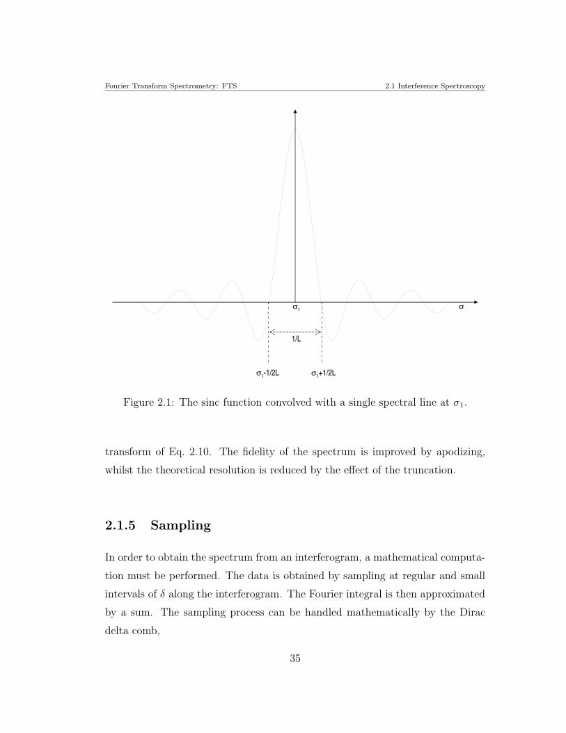
When the sinc function is convolved with a single narrow feature of the true
spectrum, the result is the sinc function centered at the wavenumber σ1, hence
the narrow spectral line is smoothed (see Fig. 2.1). The two first zeros of the
sinc function occurs at σ1 ± 1/2L. Thus two spectral lines separated by 1/L are
completely resolved. The above is the basic definition of the spectral resolution,
and is given by the maximum path difference in the interferogram. The trun-
cation function D(δ) has a sudden cutoff which introduces side-lobes near sharp
spectral features. This process, known as apodization, reduces the side-lobes, but
sacrifices the result resolution given by L.
2.1.4 Computation of the spectrum
The expression 2.11 is the density power spectrum, and 2.10 is the autocorrelation
function defining the square of the amplitude function; i.e. |Φ|2 = I(δ), and
therefore
I(σ) =
∫
−∞
+∞
|Φ|2 exp(−2πiσδ)dδ (2.14)
Since |Φ|2 is the product of a function times itself, the Fourier transform is the
convolution of the Fourier transform of the function with itself. The calculation
of the spectrum from a sampled interferogram can be performed by a Fourier
series approximation or in a more convenient way, by taking the inverse Fourier
34
Fourier Transform Spectrometry: FTS 2.1 Interference Spectroscopy
1/L
σ1-1/2L σ1+1/2L
σ1 σ
Figure 2.1: The sinc function convolved with a single spectral line at σ1.
transform of Eq. 2.10. The fidelity of the spectrum is improved by apodizing,
whilst the theoretical resolution is reduced by the effect of the truncation.
2.1.5 Sampling
In order to obtain the spectrum from an interferogram, a mathematical computa-
tion must be performed. The data is obtained by sampling at regular and small
intervals of δ along the interferogram. The Fourier integral is then approximated
by a sum. The sampling process can be handled mathematically by the Dirac
delta comb,
35
Fourier Transform Spectrometry: FTS 2.1 Interference Spectroscopy
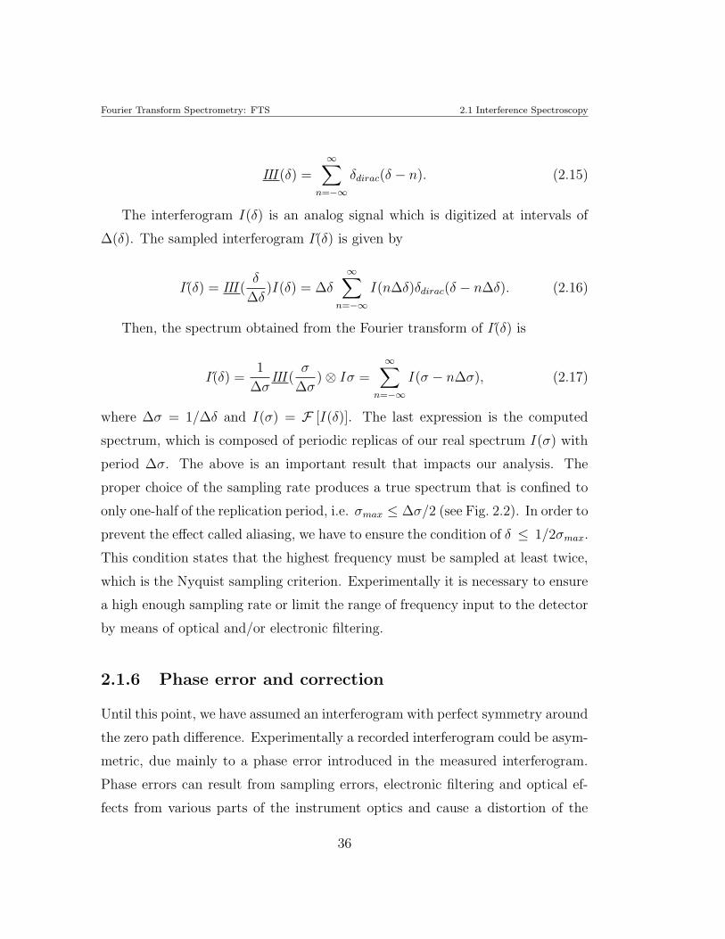
III(δ) =∞
∑
n=−∞
δdirac(δ − n). (2.15)
The interferogram I(δ) is an analog signal which is digitized at intervals of
∆(δ). The sampled interferogram I(δ) is given by
I(δ) = III(δ
∆δ)I(δ) = ∆δ
∞∑
n=−∞
I(n∆δ)δdirac(δ − n∆δ). (2.16)
Then, the spectrum obtained from the Fourier transform of I(δ) is
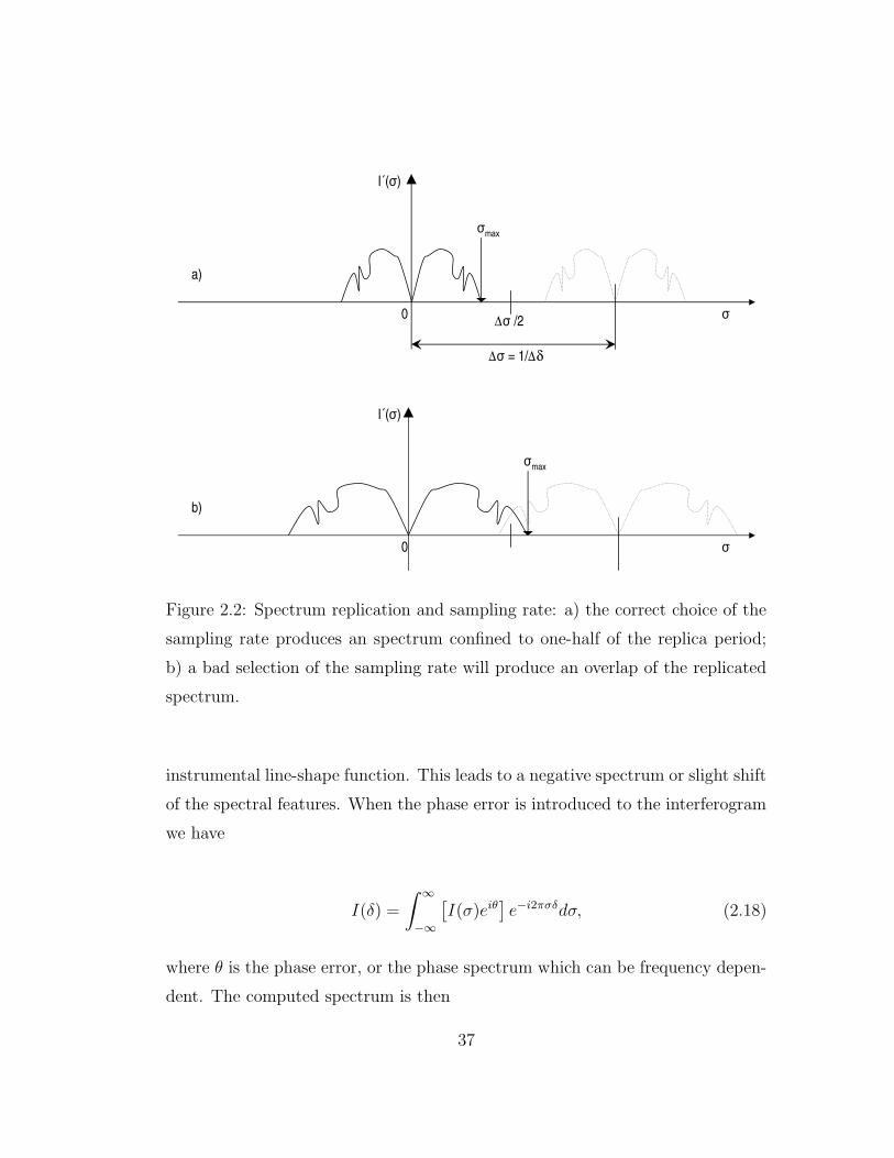
I(δ) =1
∆σIII(
σ
∆σ) ⊗ Iσ =
∞∑
n=−∞
I(σ − n∆σ), (2.17)
where ∆σ = 1/∆δ and I(σ) = F [I(δ)]. The last expression is the computed
spectrum, which is composed of periodic replicas of our real spectrum I(σ) with
period ∆σ. The above is an important result that impacts our analysis. The
proper choice of the sampling rate produces a true spectrum that is confined to
only one-half of the replication period, i.e. σmax ≤ ∆σ/2 (see Fig. 2.2). In order to
prevent the effect called aliasing, we have to ensure the condition of δ ≤ 1/2σmax.
This condition states that the highest frequency must be sampled at least twice,
which is the Nyquist sampling criterion. Experimentally it is necessary to ensure
a high enough sampling rate or limit the range of frequency input to the detector
by means of optical and/or electronic filtering.
2.1.6 Phase error and correction
Until this point, we have assumed an interferogram with perfect symmetry around
the zero path difference. Experimentally a recorded interferogram could be asym-
metric, due mainly to a phase error introduced in the measured interferogram.
Phase errors can result from sampling errors, electronic filtering and optical ef-
fects from various parts of the instrument optics and cause a distortion of the
36
Fourier Transform Spectrometry: FTS 2.1 Interference Spectroscopy
a)
b)
∆ = 1/∆δ
∆ /20
max
max
I´()
I´()
0
Figure 2.2: Spectrum replication and sampling rate: a) the correct choice of the
sampling rate produces an spectrum confined to one-half of the replica period;
b) a bad selection of the sampling rate will produce an overlap of the replicated
spectrum.
instrumental line-shape function. This leads to a negative spectrum or slight shift
of the spectral features. When the phase error is introduced to the interferogram
we have
I(δ) =
∫
∞
−∞
[
I(σ)eiθ]
e−i2πσδdσ, (2.18)
where θ is the phase error, or the phase spectrum which can be frequency depen-
dent. The computed spectrum is then
37
Fourier Transform Spectrometry: FTS 2.1 Interference Spectroscopy
I(σ) = I(σ)eiθ. (2.19)
Therefore, an asymmetric interferogram produces a complex spectrum. The
phase spectrum can be corrected using the Mertz method, Mertz 1965, which is
the most commonly scheme used. The instrumental phase is determined taking
a small symmetric sample of the interferogram about the central fringe and then
performing Fourier transform on this sample. The result is a low-resolution, high
signal-to-noise computed spectrum, which is normalized to its maximum. Using
the real and imaginary of the high S/N computed spectrum we obtain the phase
spectrum as
θ(σ) = arctan=(σ)
<(σ). (2.20)
The conjugate of this phase spectrum e−iθ(σ) is then multiplied by the Fourier
transformed spectrum of the full interferogram in order to obtain the computed
phase-corrected spectrum of the source I(σ).
2.1.7 Interferogram scanning methods
Commonly there are two kind of interferometers depending of the scanning me-
thod: step-scan interferometer and rapid-scan interferometer. In the step-scan-
ning method, the movable mirror, on a motorized track, starts from a reference
point and steps to equidistant points along the linear track. At each point the
movable mirror is kept stationary and the detector signal is recorded. The mov-
able mirror proceeds along the track until the desired resolution is achieved. The
step-scan method has an unavoidable downtime (overhead) while moving from
one sampling point to the next, and whilst waiting for the mirror position to
stabilize, before acquiring the signal. This approach takes a longer time to com-
plete a single scan than a continuous movement,and therefore it is sensitive to
38
Fourier Transform Spectrometry: FTS 2.2 Martin Puplett Interferometer
slow variations in the source intensity and instability in the detector and readout
electronics.
In the rapid-scan method the movable mirror moves at constant velocity along
the linear track. This method modulates the incoming signal at a frequency ν
which is related to the mirror velocity ν,
ν =ν
λ= νσ, (2.21)
An important factor in the rapid-scan system is the determination of the
correct time to start the data acquisition. This information is required because
the analysis method relies on the co-adding (synchronization) of various low S/N
interferograms. The S/N ratio increases as the square root of the number of scans
co-added.
2.2 Martin Puplett Interferometer
The Martin-Puplett Interferometer (here after, MPI) is a version of the Michelson
interferometer that uses wire-grid polarizers as beam splitters and roof mirrors
for reflectors. The MPI has been used widely in FIR spectroscopy and in astro-
physical spectroscopy. The MPI provides two input ports; one of them could be
used with a blackbody source of known temperature in order to have an absolute
intensity calibration. In addition, the MPI provides two output ports which are
complementary and hence the output signals can be subtracted to cancel any
common-mode noise. The MPI is an absolute interferometer because the DC off-
set component is removed. One of the main advantages of the wire-grid polarizers
is the flat broad-band spectral response.
39
Fourier Transform Spectrometry: FTS 2.2 Martin Puplett Interferometer
2.2.1 Wire grid polarizer
A wire-grid polarizer consists of many parallel wires separated by a small distance
in the plane of the grid. The physical properties of the polarizing grids designed
and fabricated for this experiment (i.e dimensions, wire-spacing, material, etc)
are described in chapter 5. When the light enters the polarizer, the component
parallel to the wire grid will induce a current along the wires. Therefore, all the
wires act as a solid metallic surface, which reflects that portion of the incoming
light with a 180 degree phase shift. The perpendicular portion of the incoming
light will not introduce a significant current in the transverse direction of the
wires, and therefore this component is unaffected and the light will be transmitted
through the polarizer. Hence, if the incoming light is polarized in a particular
direction, say horizontally, and is incident on a polarizer oriented at an angle of 45
degrees respected to the incoming light, then half of the light will be transmitted
and half will be reflected. For the case in which half of the light is reflected, a 180
degree phase shift occurs and the transmitted portion is unaffected. Thus both
the reflected and the transmitted components are 180 degrees out of phase.
2.2.2 Roof mirror
A roof mirror is a pair of plane metal surfaces placed at 90 degrees to one another.
The intersection line formed by the two planes is called the roof line. The effect of
a roof mirror is to reflect the incoming light which is perpendicular to the roof line
in the direction of incidence. The roof mirror also rotates the polarization by 2φ,
where φ is the angle between the roof line and the incident polarization direction.
If the resulting direction of polarization after passing through the polarizer is 45
degrees, then the polarization shift is 90 degrees.
40
Fourier Transform Spectrometry: FTS 2.3 Polarization through the interferometer
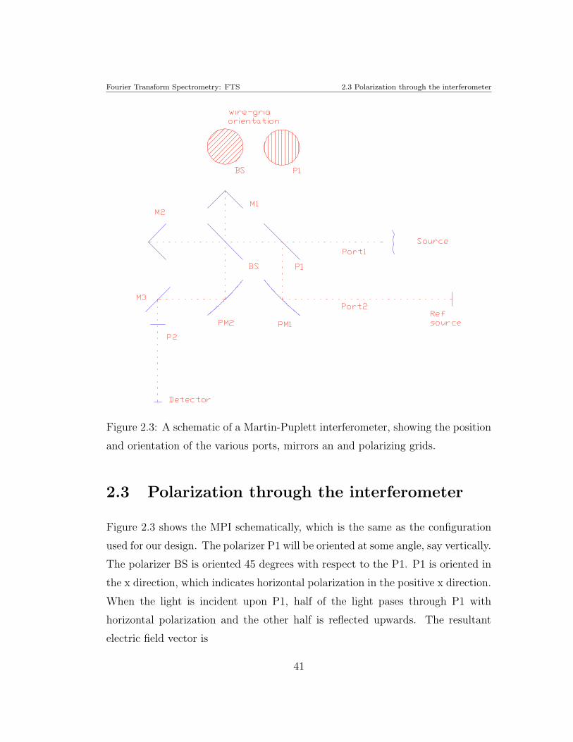
Figure 2.3: A schematic of a Martin-Puplett interferometer, showing the position
and orientation of the various ports, mirrors an and polarizing grids.
2.3 Polarization through the interferometer
Figure 2.3 shows the MPI schematically, which is the same as the configuration
used for our design. The polarizer P1 will be oriented at some angle, say vertically.
The polarizer BS is oriented 45 degrees with respect to the P1. P1 is oriented in
the x direction, which indicates horizontal polarization in the positive x direction.
When the light is incident upon P1, half of the light pases through P1 with
horizontal polarization and the other half is reflected upwards. The resultant
electric field vector is
41
Fourier Transform Spectrometry: FTS 2.3 Polarization through the interferometer
Ei = Asin
(
2πct
λ
)
x, (2.22)
where A is the amplitude of the field. The light that comes from PM1 and
is incident at P1 will also enter the interferometer by reflection. After passing
through the P1 the light strikes BS. Half the light is transmitted through the
beam splitter and half is reflected. The transmitted light now has a electric field
vector of
Et =1
2Asin
(
2πct
λ
)
(x + y). (2.23)
The transmitted light is incident on the roof mirror M2 which reflects the
light back with a phase shift of 90 degrees and returns to BS. At this point the
light has a traveled a distance d1, which is the round-trip distance from BS to
M2. The electric field vector is
Et =1
2Asin
(
2π(ct + d1)
λ
)
(x − y). (2.24)
On the other hand, the light which is reflected towards M1 from BS has an
electric field vector of
Er =1
2Asin
(
2πct
λ+ π
)
(x − y). (2.25)
where the polarization is −45 degrees, and a 180 degree phase shift is intro-
duced by the BS reflection. The light travels toward M1, and the polarization
angle is now shifted 90 degrees. The light has travelled a round trip distance d2
from BS to M1. Thus, the electric field vector is
Er =1
2Asin
(
2π(ct + d2)
λ+ π
)
(x + y), (2.26)
when the light returns to BS. Now, the light beams are incident on BS. The beam
that comes from M2 will now reflect and a 180 degree phase shift is introduced
with respect to the light leaving BS. The electric field vector is
42
Fourier Transform Spectrometry: FTS 2.3 Polarization through the interferometer
Etr =1
2Asin
(
2π(ct + d1)
λ+ π
)
(x − y). (2.27)
The light that comes from M1 is now transmitted through BS. The electric
field vector is unaltered. We can write this vector as
Ert =1
2Asin
(
2π(ct + d2)
λ+ π
)
(x + y). (2.28)
The two beams leave BS in parallel and continue toward the mirror PM2 and
eventually the detector. The total field Etot is therefore the sum of Etr and Ert
Etot = Asin
(
π(2ct − d1 − d2)
λ+ π
)
cos
(
π(d1 − d2)
λ
)
x
+ Acos
(
π(2ct − d1 − d2)
λ+ π
)
sin
(
π(d1 − d2)
λ
)
y.
(2.29)
Note that the first term in both components have an argument of ( π(2ct−d1−d2)λ
+ π); the sine term will be zero when 2ct − d1 − d2 is an integral number of
wavelengths, and the cosine term will be zero when 2ct−d1−d2 is a half number of
wavelengths. The argument in the second term of both components is(
π(d1−d2)λ
)
.
The sine term will be zero when (d1 − d2) is an integral number of wavelengths
and similarly the cosine term will be also zero when (d1 − d2) is a half number
of wavelengths.
A MPI system is able to work with two input ports and two output ports. If
there is a load present in the system in both input ports, then the radiation from
this load will enter the interferometer by transmission and reflection at P1. In our
analysis P1 is oriented vertically. The radiation from a load placed to the right
of P1 will be transmitted, and a load placed below P1 (after being collimated
by PM1) will be reflected. The transmitted component will have a horizontal
polarization and the reflected component will have vertical polarization. Then,
the two components will sum after P1, producing unpolarized light. When this
43
Fourier Transform Spectrometry: FTS 2.3 Polarization through the interferometer
unpolarized light is incident on BS, it will split and recombine such that the
beam will be unpolarized after leaving BS. The sum of the contribution of both
the horizontal and vertical polarized components after BS will be
ET = A
sin
(
π(2ct − d1 − d2)
λ
)
cos
(
π(d1 − d2)
λ
)
+ cos
(
π(2ct − d1 − d2)
λ
)
sin
(
π(d1 − d2)
λ
)
(x + y).
(2.30)
The incident light on the detector is one half of the light leaving BS, no
matter the orientation of P2. The light from the load will affect the absolute
measurement of the intensity in a constant way as long as the load source is
unpolarized, isotropic and uniform in time.
Up to here, we have reviewed the basics of the Fourier transform spectroscopy.
The importance of this brief resume, it is to put into the context the basics math-
ematical expression to understand the influence of the aspects such as, maxi-
mum optical path difference L, sampling intervals δ and scanning methods (i.e.
continuous-scan and step-integrate scan). We have also described the main ele-
ments of the Martin-Puplett interferometer, which allows us to understand how
the elements affect the radiation entering the interferometer. This previous knowl-
edge will give the tools for the design of the FTS system, which is described in
Chapter 5.
44
Chapter 3
Bolometer theory for
millimeter-wave detectors
There are a wide variety of detectors used in astronomy, which act mainly as
the transducer of the incoming radiation. The detectors can be categorized by
the physical process used to convert the electromagnetic radiation into an elec-
trical variable. In essence, there are three techniques: (i) photoelectric effect; (ii)
induced current by electromagnetic radiation, and (iii) thermal effects.
The photoelectric detection is achieved by generation of energy carriers in the
detector due to the incidence of a photon. The detection of a single photon is
possible if the energy exceeds several MeV i.e. at wavelengths larger than 200
µm. Devices based on a photoelectric effect are used over a wide spectral-range,
that goes from X-rays to mid infrared wavelengths.
Detectors which convert the electromagnetic field into current are also called
“no quantum” detectors. The electromagnetic field is coupled to an antenna,
which produces a current, which is then applied a non-linear element, i.e. a
Shottky diode. These detectors are usable throughout the whole radio and sub-
45
Bolometer theory for millimeter-wave detectors Bolometer theory for millimeter-wave detectors
mm/mm wavelength range.
The detectors based on thermal effect absorb the photon energy and transform
it into thermal excitation. The incident radiation can be detected by the small
temperature drift produced by the excitation. These detectors are mainly used at
infrared and sub-mm/mm wavelengths as bolometers, as well as in the X-ray and
gamma-ray regimes as calorimeters. Due to their broad-band spectral response,
bolometers are also the most suitable as detectors for spectroscopy (i.e. as part
of an FTS).
The Fourier transform spectrometer described in this thesis will be used to
measure the sub-mm/mm atmospheric emission and calculate the transmission
spectrum of the atmosphere and other materials, such as bandpass filters. We
have chosen to use a bolometer as the detector in a cryogenic system operating at
∼ 1.8 or 3.9 K. The FTS-MPI is designed to work over a frequency range of ∼ 215
to 2000 GHz. The estimated sky background power that falls on the bolometer
continuously is 30× 10−9 W. For an operating temperature is 1.8 K, the required
noise equivalent power (NEP) of the detector under background limited operation
is ∼ 10−15 WHz−1/2. These parameters drive the design and performance of the
bolometer, which are described in chapter 4, as well as the results of the electrical
characterization of the cryogenic detector system.
In this chapter we describe bolometer theory and their basic principles of op-
eration. We focus our attention on those devices that use Neutron Transmutation
Doped Germanium (NTD Ge here after) thermistors. The theory has been devel-
oped and reported by other authors (e.g. Low 1961; Mather 1982; Richards 1994),
and therefore only a brief review of the theory for ideal bolometers is given here.
The experimental characterization of our cryogenic bolometer system is described
in chapter 4.
46
Bolometer theory for millimeter-wave detectors 3.1 An ideal Bolometer
3.1 An ideal Bolometer
A bolometer is a thermal device, which does not detect photons by means of an
excitation of the charge carriers, but instead it detects a thermal variation which
is proportional to the energy absorbed from the photons. Typically bolometers
have a broadband spectral response that is defined by the properties of the ab-
sorber material used. Bolometers are the most suitable devices for applications
in the infrared and sub-mm/mm spectral range (since stressed photoconductors
reach their limits at ∼ 200µm). The germanium crystal was the first thermome-
ter, (Low, 1961) to be developed for operation at low temperature. Currently the
most popular thermometer elements are those made by the NTD process, which
produces more uniform doping through the semiconductor crystal.
Semiconductor bolometers have been used successfully in astronomical obser-
vations in the past, although they will become increasingly replaced by a new
generation of devices in the future. The increasing research effort into the devel-
opment of superconducting detectors and into micro-machining techniques have
now made it possible to construct large-format detectors array (i.e. ≥ 1000 pix-
els). The next generation of instruments (e.g. SCUBA-2) will be based on the
Superconducting Transition Edge Sensor (TES) array that will work mapping the
focal plane of the telescope as fast as a CCD or IR array does.
TES detectors are made of a superconducting film that works in the transition
temperature region TC , between the superconducting and normal state. The
resistance has a very steep dependence on temperature as shown in Figure 3.1.
Small changes in temperature will produce a large change in resistance. These
devices are voltage biased, so that the change in resistance produces a change
in the current through the superconducting film, which is measured with a very
sensitive ammeter (i.e. Superconducting Quantum Interference Devices, SQUID).
47
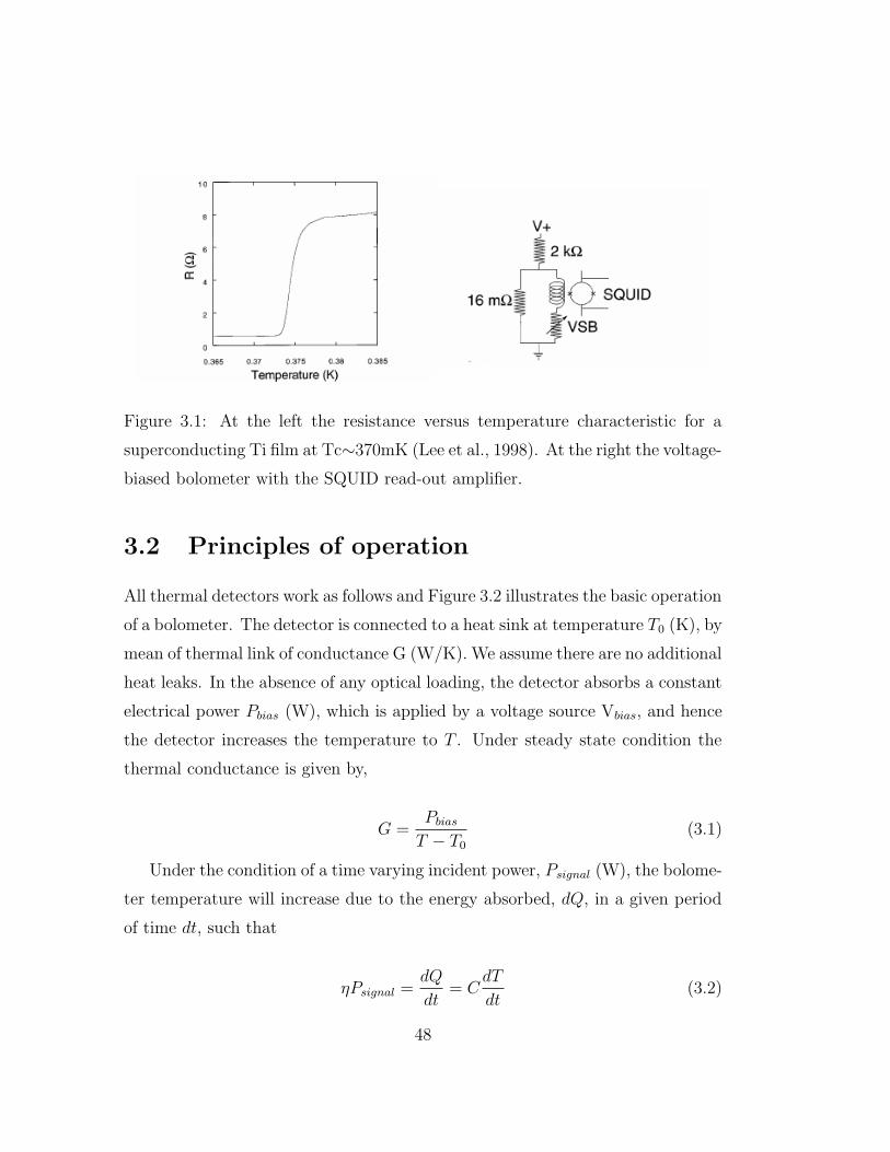
Bolometer theory for millimeter-wave detectors 3.2 Principles of operation
Figure 3.1: At the left the resistance versus temperature characteristic for a
superconducting Ti film at Tc∼370mK (Lee et al., 1998). At the right the voltage-
biased bolometer with the SQUID read-out amplifier.
3.2 Principles of operation
All thermal detectors work as follows and Figure 3.2 illustrates the basic operation
of a bolometer. The detector is connected to a heat sink at temperature T0 (K), by
mean of thermal link of conductance G (W/K). We assume there are no additional
heat leaks. In the absence of any optical loading, the detector absorbs a constant
electrical power Pbias (W), which is applied by a voltage source Vbias, and hence
the detector increases the temperature to T . Under steady state condition the
thermal conductance is given by,
G =Pbias
T − T0
(3.1)
Under the condition of a time varying incident power, Psignal (W), the bolome-
ter temperature will increase due to the energy absorbed, dQ, in a given period
of time dt, such that
ηPsignal =dQ
dt= C
dT
dt(3.2)
48
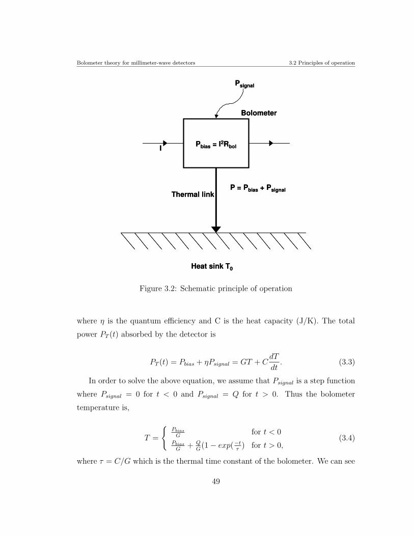
Bolometer theory for millimeter-wave detectors 3.2 Principles of operation
Heat sink T0
Thermal linkP = Pbias + Psignal
Psignal
Pbias = I2RbolI
Bolometer
Heat sink T0
Thermal linkP = Pbias + Psignal
Psignal
Pbias = I2RbolI
Bolometer
Figure 3.2: Schematic principle of operation
where η is the quantum efficiency and C is the heat capacity (J/K). The total
power PT (t) absorbed by the detector is
PT (t) = Pbias + ηPsignal = GT + CdT
dt. (3.3)
In order to solve the above equation, we assume that Psignal is a step function
where Psignal = 0 for t < 0 and Psignal = Q for t > 0. Thus the bolometer
temperature is,
T =
Pbias
Gfor t < 0
Pbias
G+ Q
G(1 − exp(−t
τ) for t > 0,
(3.4)
where τ = C/G which is the thermal time constant of the bolometer. We can see
49
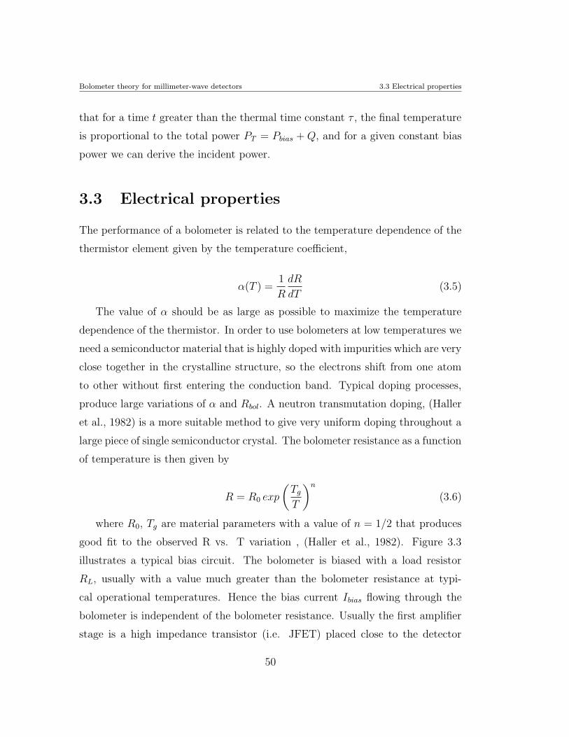
Bolometer theory for millimeter-wave detectors 3.3 Electrical properties
that for a time t greater than the thermal time constant τ , the final temperature
is proportional to the total power PT = Pbias + Q, and for a given constant bias
power we can derive the incident power.
3.3 Electrical properties
The performance of a bolometer is related to the temperature dependence of the
thermistor element given by the temperature coefficient,
α(T ) =1
R
dR
dT(3.5)
The value of α should be as large as possible to maximize the temperature
dependence of the thermistor. In order to use bolometers at low temperatures we
need a semiconductor material that is highly doped with impurities which are very
close together in the crystalline structure, so the electrons shift from one atom
to other without first entering the conduction band. Typical doping processes,
produce large variations of α and Rbol. A neutron transmutation doping, (Haller
et al., 1982) is a more suitable method to give very uniform doping throughout a
large piece of single semiconductor crystal. The bolometer resistance as a function
of temperature is then given by
R = R0 exp
(
Tg
T
)n
(3.6)
where R0, Tg are material parameters with a value of n = 1/2 that produces
good fit to the observed R vs. T variation , (Haller et al., 1982). Figure 3.3
illustrates a typical bias circuit. The bolometer is biased with a load resistor
RL, usually with a value much greater than the bolometer resistance at typi-
cal operational temperatures. Hence the bias current Ibias flowing through the
bolometer is independent of the bolometer resistance. Usually the first amplifier
stage is a high impedance transistor (i.e. JFET) placed close to the detector
50
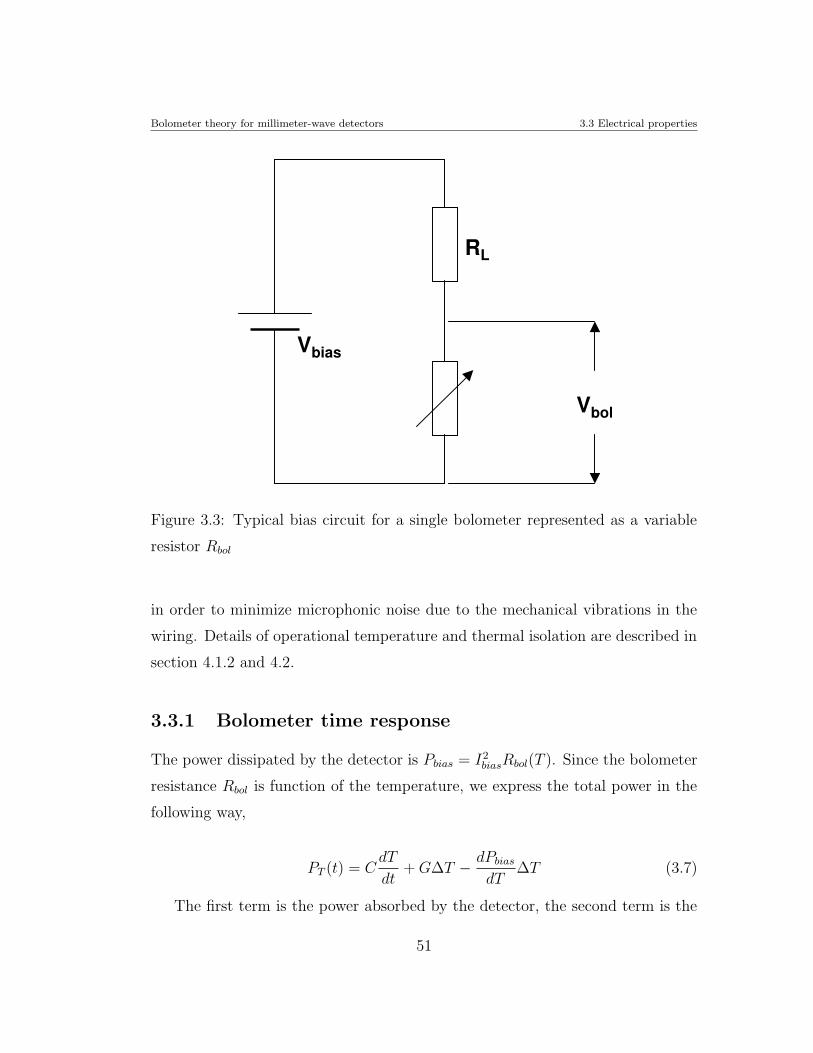
Bolometer theory for millimeter-wave detectors 3.3 Electrical properties
Vbol
RL
Vbias
Figure 3.3: Typical bias circuit for a single bolometer represented as a variable
resistor Rbol
in order to minimize microphonic noise due to the mechanical vibrations in the
wiring. Details of operational temperature and thermal isolation are described in
section 4.1.2 and 4.2.
3.3.1 Bolometer time response
The power dissipated by the detector is Pbias = I2biasRbol(T ). Since the bolometer
resistance Rbol is function of the temperature, we express the total power in the
following way,
PT (t) = CdT
dt+ G∆T − dPbias
dT∆T (3.7)
The first term is the power absorbed by the detector, the second term is the
51
Bolometer theory for millimeter-wave detectors 3.3 Electrical properties
bias power and third is the dissipated power by the detector resistance Rbol. The
change in the power due to a change in the temperature is expressed as,
dP
dT= I2 dRbol
dT(3.8)
where dRbol
dT= R0α(T ), and hence
dP
dT= α(T )Pbias (3.9)
Substituting equation 3.9 into the expression for total power (Eq. 3.7) we
obtain
PT (t) = CdT
dt+ (G − αPbias)∆T. (3.10)
Solving this diferential equation we then obtain the electrical time constant
τe = CG−αPbias
.
When α < 0 we observe that the electrical time constant is smaller than the
thermal time constant (τ = C/G). Therefore, a bolometer responds electrically
faster than thermally which is due to the Electro thermal feedback. This effect
has the advantage to speed up the response time of the sensor.
3.3.2 Responsivity
The temperature of a bolometer increases due to absorbed radiant power. The
bolometer is also biased by a constant current, and produces additional electrical
power via the Joule effect. The bolometer dissipates the combined power through
the thermal link to the heat sink. Changes in the voltage output are related to
variations in the absorbed power. The detector responsivity is defined as the
change in the voltage output due to the absorbed input signal power, dV/dP
(V/W),
dV = IdR = IαRdT = αV dT, (3.11)
52
Bolometer theory for millimeter-wave detectors 3.3 Electrical properties
for a zero frequency response (τ >> τe) and where dT is expressed as
dT =dP
G − αPbias
(3.12)
and hence
dV =αV dP
G − αPbias
. (3.13)
The electrical responsivity of a bolometer S(0) = dV/dP is then
S(0) =αV
G − αPbias
. (3.14)
In order to measure the electrical responsivity it is necessary to derive α and
G from the V-I load curve. The dependence of the voltage on bias is not linear
due to the Joule heating of the bolometer. For a bolometer with α < 0, Vbol(I)
is linear with a slope R when Vbol ≈ 0 (low bias regime), and it also has a broad
roll over before falling slowly at larger bias currents. Experimental V-I curves are
presented in Chapter 4.
From the load curves, we are able to derive R = V/I and the impedance Z =
dV/dI. The electrical responsivity S can also be expressed in terms of R and Z
when no optical power is applied.
S(0) =(Z − R)
2IR(3.15)
Note that the responsivity of a bolometer is independent of the operation
wavelength.
3.3.3 Noise and noise equivalent power (NEP)
There are two ways to study the noise in a bolometric system. The first is un-
der assumption of thermal equilibrium. The second is using the non-equilibrium
53
Bolometer theory for millimeter-wave detectors 3.3 Electrical properties
theory developed by Mather (1982) in which the mechanism of the thermal feed-
back is taken into account. In the present work we use the thermal equilibrium
theory that is very useful for obtaining a general understanding of the bolometer
operation and its optimization.
One important figure of merit for a bolometer is the noise equivalent power
(NEP), which is a measure of the sensitivity of a bolometer, and is defined as
the power absorbed that produces a signal to noise ratio of unity at the output
(units of W/Hz1/2). The NEP is formed by taking into account the detector and
the background noise, and can be expressed as,
NEPtot =√
NEP 2detector + NEP 2
background (3.16)
In an ideal case the NEP should be limited by the thermal noise (i.e. sky
background, telescope and optics background) and not by the detector noise
contribution. In general there are two types of noise in a bolometric system. One
kind is related to the pure electrical components (i.e. Johnson noise coming from
the bolometer, load resistor and amplifier). The bolometer is subject to Johnson
noise due to the random motion of the free electrons in the thermistor element
and it is expressed as,
NEPJ =(4kTRbol)
1/2
S(3.17)
where k is the Boltzman constant, and S is responsivity in V/W. The NEPJ
is independent of the load resistance. Another source of Johnson noise comes
from the load resistors, but in the practice we reduce this contribution by using
a large load resistor RL >> Rbol at the operating temperature.
Second, noise comes from thermalization of the mechanical vibrations and
thermal fluctuations at the thermal link (i.e. electrical leads), which is produced
by the random propagation of energy carriers, (e.g. electrons, phonons, photons,
etc). These fluctuations are generally called phonon noise, and are analogous
54
Bolometer theory for millimeter-wave detectors 3.3 Electrical properties
to the Johnson noise. We consider a system with a heat capacity C connected
via a thermal link with a conductance G to a heat sink at T0 to help describe
its contribution. In thermal equilibrium the energy ET stored in the thermal
capacitance CT should be,
ET =1
2CT T 2
N (3.18)
where TN is the thermal fluctuation, and the power dissipation in the RT (where
RT is the equivalent resistance that replaces the thermal link) is
PT =T 2
N
RT
. (3.19)
We also expect the circuit to have a exponential response with a time constant
of RT CT . From τ = C/G we obtain,
CT =C
Tand RT =
T
G(3.20)
where RT is the thermal resistance. Using the the electrical analogous 〈V 2J 〉 =
(4kTR)dν, to make the analogy with the thermal variables we have,
〈T 2N〉 =
4kT 2
Gdν (3.21)
We let Pν be the power falling on the bolometer which produces a temperature
change of
∆Ts =ηPν
G(3.22)
Thus the value of Pν give us an equality between thermal fluctuations and the
signal noise,
∆Ts = 〈T 2N〉1/2 (3.23)
such that the phonon NEP in unit bandwidth is expressed as,
55
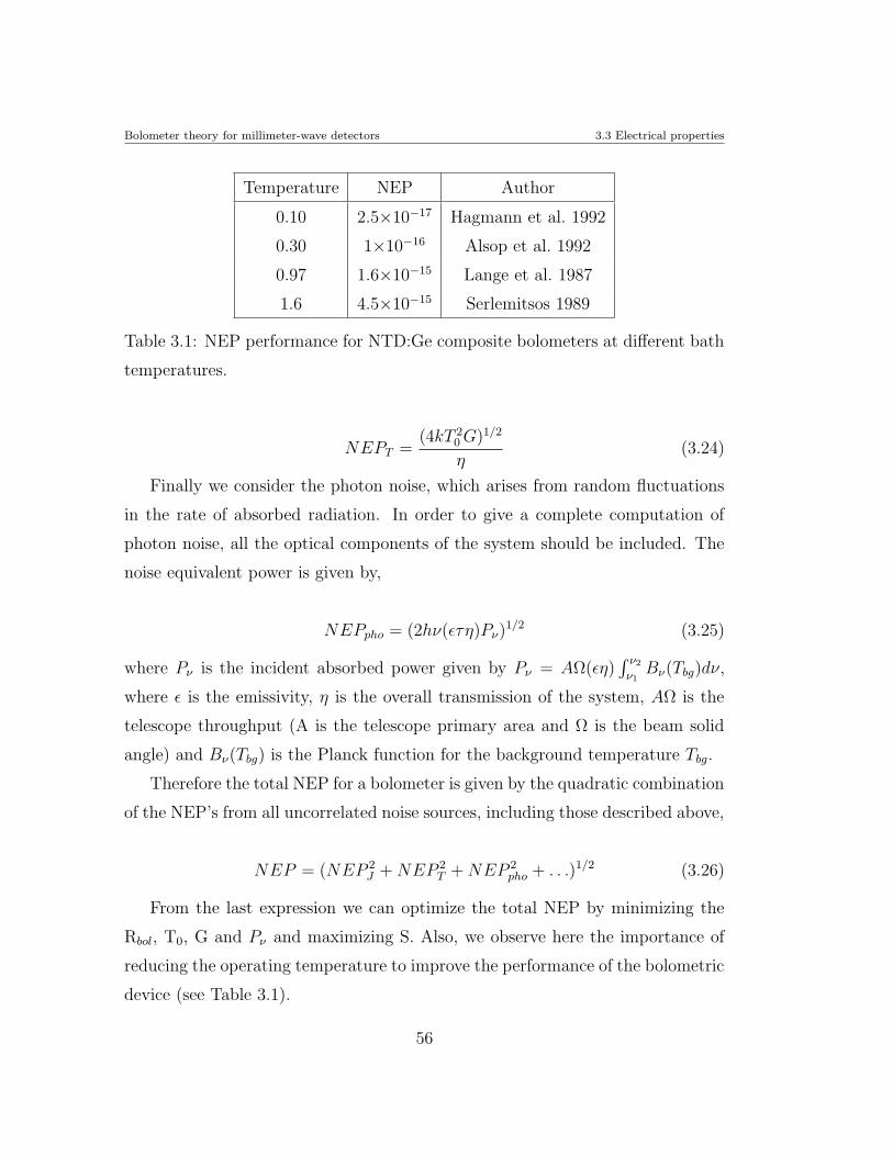
Bolometer theory for millimeter-wave detectors 3.3 Electrical properties
Temperature NEP Author
0.10 2.5×10⁻¹⁷ Hagmann et al. 1992
0.30 1×10⁻¹⁶ Alsop et al. 1992
0.97 1.6×10⁻¹⁵ Lange et al. 1987
1.6 4.5×10⁻¹⁵ Serlemitsos 1989
Table 3.1: NEP performance for NTD:Ge composite bolometers at different bath
temperatures.
NEPT =(4kT 2
0 G)1/2
η(3.24)
Finally we consider the photon noise, which arises from random fluctuations
in the rate of absorbed radiation. In order to give a complete computation of
photon noise, all the optical components of the system should be included. The
noise equivalent power is given by,
NEPpho = (2hν(ετη)Pν)1/2 (3.25)
where Pν is the incident absorbed power given by Pν = AΩ(εη)∫ ν2
ν1
Bν(Tbg)dν,
where ε is the emissivity, η is the overall transmission of the system, AΩ is the
telescope throughput (A is the telescope primary area and Ω is the beam solid
angle) and Bν(Tbg) is the Planck function for the background temperature Tbg.
Therefore the total NEP for a bolometer is given by the quadratic combination
of the NEP’s from all uncorrelated noise sources, including those described above,
NEP = (NEP 2J + NEP 2
T + NEP 2pho + . . .)1/2 (3.26)
From the last expression we can optimize the total NEP by minimizing the
Rbol, T0, G and Pν and maximizing S. Also, we observe here the importance of
reducing the operating temperature to improve the performance of the bolometric
device (see Table 3.1).
56
Bolometer theory for millimeter-wave detectors 3.4 Physical parameters
3.4 Physical parameters
3.4.1 Heat capacity
The material used as a thermistor is usually a semiconductor crystal. The specific
heat of a pure semiconductor material at low temperature is given by the Debye
theory for a crystal lattice:
clatv =
12π4ℵAk
5
(
T
ΘD
)3
, (3.27)
where ℵA is Avogadro’s number times density over atomic weight and ΘD
is the Debye temperature. For metals, cv, includes contributions both from the
lattice structure and from free electrons. The electronic specific heat is
cev = γeT (ρ mole−1), (3.28)
where γe depends on the metal and ρ is the material density. The specific
heat includes the lattice and electronic contributions, and as the temperature
approaches to zero, the major contribution is due to cev. Hence
cv = DT 3 + γeT, (3.29)
Since a bolometer is a semiconductor connected by metallic leads, the con-
tributions to its heat capacity comes from both the crystalline semiconductor
elements (C ∝ T 3) and from the electrical leads (C ∝ T ), such that
C = clatv Vlat + ce
vVe, (3.30)
where Vlat and Ve represent their respective volumes.
For temperatures above 1 K we have chosen very carefully the materials in
order to reduce the total heat capacity of our device (see Chapter 4). Another
way to minimize C is by reducing the total volume of the elements, although in
57
Bolometer theory for millimeter-wave detectors 3.4 Physical parameters
the practice the exact dimension of some components are hard to control (i.e.
glue, silver epoxy, etc.)
3.4.2 Thermal conductance
The behavior of the thermal link has a direct influence on many figures of merit
for a bolometer (e.g. NEP, time response and responsivity). The thermal conduc-
tance is dominated by the electrical leads. The thermal conductivity of metals is
described by
ke ≈ LσT (3.31)
where the term L is the Lorentz number (≈ 2.45×10⁻⁸ WΩK−2) and σ is the
electrical conductivity. The value of ke is ∼ T a, with a ≥ 1 for low temperatures
(e.g. ∼.1 - 4.2 K). Usually a bolometer is connected with two leads of length L
and cross sectional area A, so that the thermal conductance is
G = 2A
Lke. (3.32)
3.4.3 Choice of the thermistor
Usually Si and Ge semiconductors are used as the thermometer material for
bolometers operating at L4He temperatures. These devices must then be heavily
doped in order reduce the intrinsic large resistance at such low operating tem-
peratures (∼ 0.1 − 4.2 K).
Semiconductors thermistors are doped close to the metal-insulator transition
with majority impurity, in order to get a hopping conductivity mode, (Efros &
Shklovskii, 1975), which gives a temperature-dependent resistance described by
Eq. 3.6. A neutron transmutation doping (NTD) of ultra-pure Ge produces a
more uniform material that can operate effectively at temperatures from 4.2 K
58
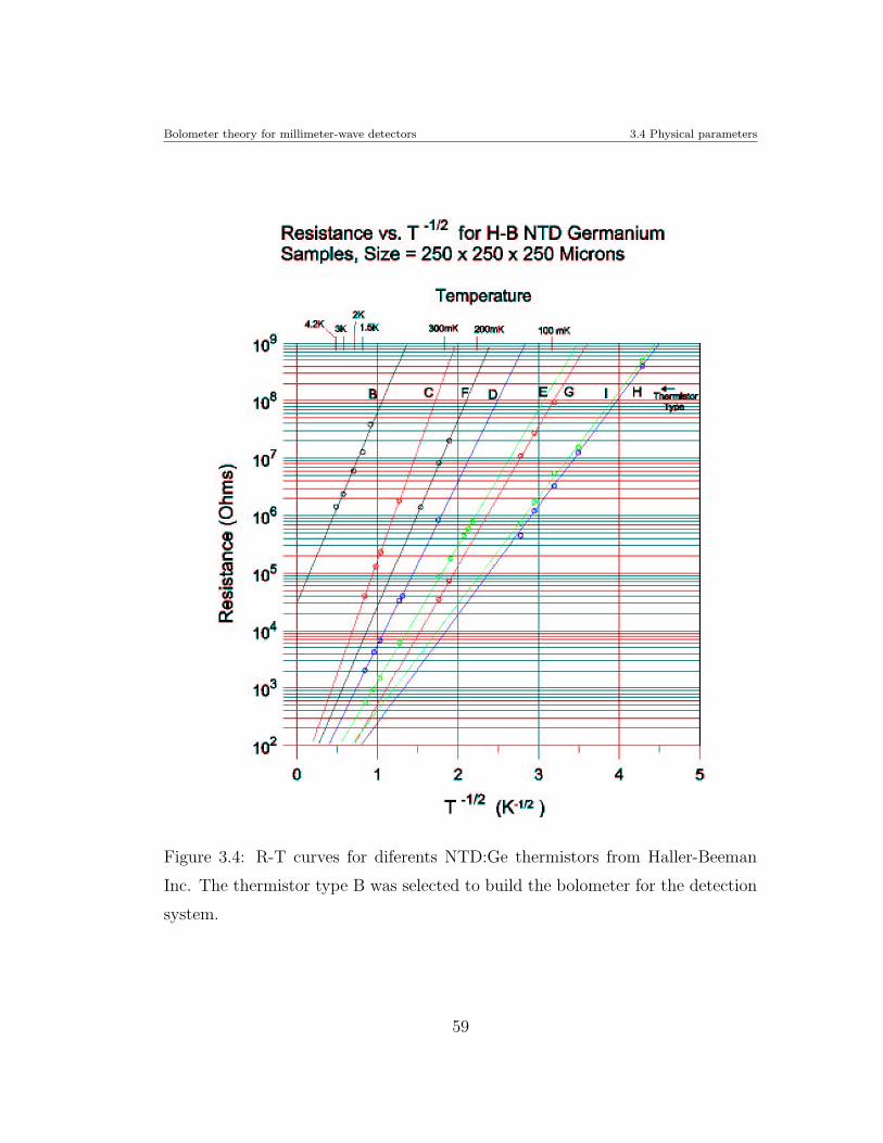
Bolometer theory for millimeter-wave detectors 3.4 Physical parameters
Figure 3.4: R-T curves for diferents NTD:Ge thermistors from Haller-Beeman
Inc. The thermistor type B was selected to build the bolometer for the detection
system.
59
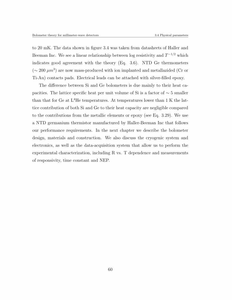
Bolometer theory for millimeter-wave detectors 3.4 Physical parameters
to 20 mK. The data shown in figure 3.4 was taken from datasheets of Haller and
Beeman Inc. We see a linear relationship between log resistivity and T−1/2 which
indicates good agreement with the theory (Eq. 3.6). NTD Ge thermometers
(∼ 200 µm3) are now mass-produced with ion implanted and metallazided (Cr or
Ti-Au) contacts pads. Electrical leads can be attached with silver-filled epoxy.
The difference between Si and Ge bolometers is due mainly to their heat ca-
pacities. The lattice specific heat per unit volume of Si is a factor of ∼ 5 smaller
than that for Ge at L4He temperatures. At temperatures lower than 1 K the lat-
tice contribution of both Si and Ge to their heat capacity are negligible compared
to the contributions from the metallic elements or epoxy (see Eq. 3.29). We use
a NTD germanium thermistor manufactured by Haller-Beeman Inc that follows
our performance requirements. In the next chapter we describe the bolometer
design, materials and construction. We also discuss the cryogenic system and
electronics, as well as the data-acquisition system that allow us to perform the
experimental characterization, including R vs. T dependence and measurements
of responsivity, time constant and NEP.
60
Chapter 4
Cryogenic Camera for the FTS
As part of the construction and testing a working sub-mm/mm FTS we decided
to design a detection system for FTS-MPI (described in Chapter 5) based on a
composite bolometer detector due to its sensitivity and low noise characteristics
over the sub-mm/mm wavelengths. In this chapter we describe the design of the
bolometer, assuming it operates under background limited conditions, and also
describe how this influences parameters such as thermal conductance and operat-
ing temperature. We also explain issues related to the overall characterization of
the cryogenic system and finally we derive the figures of merit for the bolometer.
4.1 Bolometer design
The cryogenic camera system for the FTS uses a composite bolometer, which
consists of a small thermistor element mounted in a dielectric-coated substrate.
The dielectric substrate acts as the absorber of the incident radiation. Figure 4.1
shows the general scheme for our composite bolometer, which consists of a NTD
Ge thermistor mounted on a thin square of sapphire. The absorber surface is
61
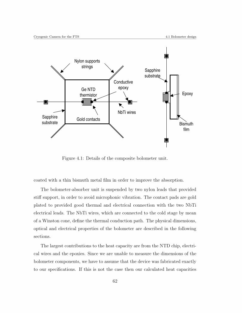
Cryogenic Camera for the FTS 4.1 Bolometer design
Ge NTDthermistor
Gold contacts
Conductive epoxy
Nylon supports strings
Sapphire substrate
NbTi wires
Bismuth film
Sapphire substrate
Epoxy
Figure 4.1: Details of the composite bolometer unit.
coated with a thin bismuth metal film in order to improve the absorption.
The bolometer-absorber unit is suspended by two nylon leads that provided
stiff support, in order to avoid microphonic vibration. The contact pads are gold
plated to provided good thermal and electrical connection with the two NbTi
electrical leads. The NbTi wires, which are connected to the cold stage by mean
of a Winston cone, define the thermal conduction path. The physical dimensions,
optical and electrical properties of the bolometer are described in the following
sections.
The largest contributions to the heat capacity are from the NTD chip, electri-
cal wires and the epoxies. Since we are unable to measure the dimensions of the
bolometer components, we have to assume that the device was fabricated exactly
to our specifications. If this is not the case then our calculated heat capacities
62
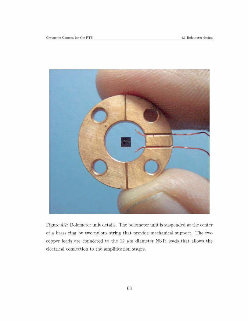
Cryogenic Camera for the FTS 4.1 Bolometer design
Figure 4.2: Bolometer unit details. The bolometer unit is suspended at the center
of a brass ring by two nylons string that provide mechanical support. The two
copper leads are connected to the 12 µm diameter NbTi leads that allows the
electrical connection to the amplification stages.
63
Cryogenic Camera for the FTS 4.1 Bolometer design
are in error. Heat capacity, thermal conductance and the operation tempera-
ture should be chosen carefully in order to give the required performance for a
given application. The next sections describe our detailed design of the composite
bolometer.
4.1.1 Detector load and sky-power conditions
The FTS has been designed with the intention and goal to measured the broad-
band spectrum of the sky above Sierra La Negra. The bolometer is designed
to work with two different experiments. The first experiment is a Total Power
Sky Monitor (Ferrusca, 2006), which measures the sky power at 250 GHz with a
bandwidth of ∼ 70 GHz. The second application, described in this thesis is the
FTS, in which the bandwidth is defined by the natural cut-off of the Winston
Cone at ∼ 200 GHz (low-frequency side) and the high-frequency cut-off of the
flourogold filter at ∼ 1000 GHz. The background power level can be calculated
as follows,
P (ν, T ) = ηεAΩB(ν, T )dν (4.1)
where η and ε are total transmission of the system and the emissivity of the
background respectively. The product AΩ is the throughput of the system and
B(ν, T ) is the Plank function. The effective Rayleigh-Jeans temperature for a
blackbody is,
J(ν, T ) =xT
ex − 1dν (4.2)
where x = hν/kT , and therefore the Plank function in terms of the effective
temperature is
B(ν, T ) =2kν2
c2J(ν, T )dν. (4.3)
We can now express the total power as follow,
P (ν, T ) = ηεAΩ2k
λ2J(ν, T )dν (4.4)
64
Cryogenic Camera for the FTS 4.1 Bolometer design
where the throughput for a broadband system is > λ2. It can be expressed as
N(λ) = 2AΩ/λ2, where N is the number of modes. In general the power absorbed
by the detector is,
P (ν, T ) = ηεN(λ)kJ(ν, T )dν (4.5)
The estimated sky-background power for sky-temperature of 270K is 20.7 ×10⁻⁹ W and the optical background power is 8.2×10⁻⁹ W for the useful bandwidth
of ∼ 200 to 1000 GHz. Hence the expected total background power is ∼ 30×10−9
W.
4.1.2 Operational temperature
Once the background power is estimated, we have to choose the operation tem-
perature T0. The choice of the operation temperature is not a trivial task because
T0 has a direct influence on the bolometer sensitivity and noise performance. Also
the choice will depend on the refrigeration system available. Typical refrigeration
systems are: an open system of liquid helium (L4He), for temperatures of ∼ 4.2
K; pumped L4He for range of temperatures ∼ 1.8 − 1.2 K (depending on the
vacuum level); a closed cycle system of L3He for temperatures of ∼ 300 − 200
mK; a L4He/L3He dilution refrigerator and adiabatic demagnetization refrigera-
tor with temperatures as low as ∼ 100 mK. The contribution to the NEP depends
strongly with the bath temperature T0. In the case of a constant background the
NEP goes as ∝ T 1/2. The photon noise is independent of the temperature. In
the case that T0 has been chosen to keep a given frequency response, the NEP
∝ T 5/2. Finally the choice should be driven by increasing the responsivity, where
R ∝ NEP−1, in order to minimize the Johnson noise and amplifier noise.
Due to the strict financial limitations we have designed the bolometer to
work in a temperature range of ∼1.6 K - 4.2 K, since a colder, more sensitive
300 mK system costs ∼ 50,000 USD. The cryogenic system of the MI-LAB is a
liquid helium cryostat, in which is possible to pump directly on the liquid helium
65
Cryogenic Camera for the FTS 4.1 Bolometer design
reservoir to obtain a T0 < 4.2 K. By reducing the vapor pressure above the liquid,
temperatures down to 1.2 K can be obtained. Our system system is able to attain
a stable temperature at 1.8 K.
4.1.3 Thermal conductance
In general the thermal conductance G of the thermal link depends on the tem-
perature gradient, cross-sectional area, length and material composition. The
temperature distribution along the thermal link will depend on the bolometer
temperature Tb and the heat sink temperature T0. By the definition the power
passing through the thermal link is equal to the thermal conductance times the
temperature difference across the link (Eq. 3.1). Eq. 3.32 relates the geometry
and material composition of the thermal link, which is used to design a given
value for G. In order to determine G in terms of a constant background power
i.e. Q = P , we set a temperature rise ratio (Tb − T0)/T0 = 0.5, where Tb is the
bolometer temperature. Under that condition the required thermal conductance
is calculated using the next expression,
G =2Q
T0
, (4.6)
and hence the thermal conductance is G ≈ 3 × 10⁻⁸ W/K. The electrical leads
dominate the thermal conductance in a bolometer. Then choice of the electrical
leads is driven by the required value of G. Nevertheless there is not a wide variety
of materials and it is not easy to select a suitable one.
We chose to use copper clad NbTi wires as the electrical leads. This material
has been characterized partially at temperatures below 1 K. Reported values of
G are: 4.7× 10⁻¹⁰ W/K at 375 mK Lee et al. (1998), 7× 10⁻¹¹ W/K at 315 mK
Mauskopf et al. (1997), and a G∼ 1× 10⁻⁹ W/K at 4.2 K is reported (Lakeshore
Inc. datasheet). From a linear interpolation to the thermal conductivity, we ob-
tained a G≈ 3×10⁻⁹ W/K, which is ∼ 10 times lower than the required G under
66
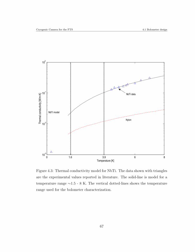
Cryogenic Camera for the FTS 4.1 Bolometer design
0 6 81.6 3.910-3
10-2
10-1
100
Temperature [K]
Ther
mal
con
duct
ivity
[W/m
-K]
Nylon
NbTi model
NbTi data
Figure 4.3: Thermal conductivity model for NbTi. The data shown with triangles
are the experimental values reported in literature. The solid-line is model for a
temperature range ∼1.5 - 8 K. The vertical dotted-lines shows the temperature
range used for the bolometer characterization.
67
Cryogenic Camera for the FTS 4.1 Bolometer design
constant background conditions. The absorber-thermistor unit is suspended by
two additional nylon supports, which have negligible contribution to the total
thermal conductivity, therefore the total thermal conductance estimated for our
bolometer at 1.8 K is ∼ 3× 10⁻⁹ W/K. Figure 4.3 shows the thermal conductiv-
ity of the materials used for the bolometer construction and this quantities are
geometrically related with the thermal conductance.
4.1.4 Heat capacity and time constant
The total heat capacity is an important value because it defines the frequency
response of our device (τ = C/G). The area of a bolometer must be larger in
order to maximize the absorption efficiency of the signal. A large area however will
simultaneously increase the volume of the absorber unit and therefore the heat
capacity of the bolometer. The larger the value of C, the slower the response time.
The most significant contributions to the heat capacity are from the bolometer
(i.e. thermistor plus absorber) and thermal epoxy. The values for the various
heat capacities given in table 4.1 are uncertain due to the exact geometry of the
components. For example, the application of thermal and conductive epoxies is
difficult to control during the construction of the bolometer.
The total heat capacity of the bolometer is ∼ 2 × 10⁻⁹ J/K and hence, when
operating at 1.8 K, the maximum frequency response is ∼ 1.5 Hz. The above is a
disadvantage for the performance of the FTS-MPI. This slow response will affect
the scan-speed increasing the time to record single interferogram. Therefore we
are no sensitive to time scales lower than the time constant τ .
4.1.5 The bolometer absorber
The absorber has the function of improving the effective area of the bolometer
and the absorption properties over the sub-mm/mm range. The absorber is a thin
metallic film of bismuth with a sheet resistance R2 deposited on a thin transparent
68
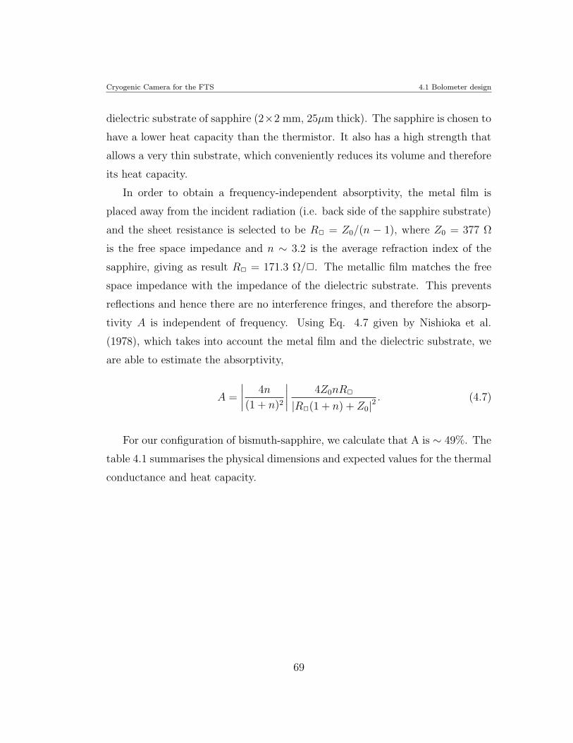
Cryogenic Camera for the FTS 4.1 Bolometer design
dielectric substrate of sapphire (2×2 mm, 25µm thick). The sapphire is chosen to
have a lower heat capacity than the thermistor. It also has a high strength that
allows a very thin substrate, which conveniently reduces its volume and therefore
its heat capacity.
In order to obtain a frequency-independent absorptivity, the metal film is
placed away from the incident radiation (i.e. back side of the sapphire substrate)
and the sheet resistance is selected to be R2 = Z0/(n − 1), where Z0 = 377 Ω
is the free space impedance and n ∼ 3.2 is the average refraction index of the
sapphire, giving as result R2 = 171.3 Ω/2. The metallic film matches the free
space impedance with the impedance of the dielectric substrate. This prevents
reflections and hence there are no interference fringes, and therefore the absorp-
tivity A is independent of frequency. Using Eq. 4.7 given by Nishioka et al.
(1978), which takes into account the metal film and the dielectric substrate, we
are able to estimate the absorptivity,
A =
∣
∣
∣
∣
4n
(1 + n)2
∣
∣
∣
∣
4Z0nR2
|R2(1 + n) + Z0|2. (4.7)
For our configuration of bismuth-sapphire, we calculate that A is ∼ 49%. The
table 4.1 summarises the physical dimensions and expected values for the thermal
conductance and heat capacity.
69
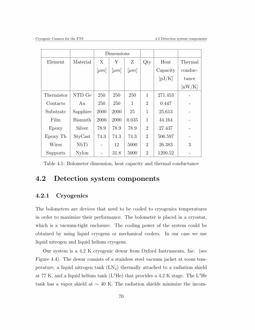
Cryogenic Camera for the FTS 4.2 Detection system components
Dimensions
Element Material X Y Z Qty Heat Thermal
[µm] [µm] [µm] Capacity conduc-
[pJ/K] tance
[nW/K]
Thermistor NTD Ge 250 250 250 1 271.453 -
Contacts Au 250 250 1 2 0.447 -
Substrate Sapphire 2000 2000 25 1 25.613 -
Film Bismuth 2000 2000 0.035 1 44.164 -
Epoxy Silver 78.9 78.9 78.9 2 27.437 -
Epoxy Th StyCast 74.3 74.3 74.3 2 506.597 -
Wires NbTi - 12 5000 2 26.383 3
Supports Nylon - 31.8 5000 2 1200.52 -
Table 4.1: Bolometer dimension, heat capacity and thermal conductance
4.2 Detection system components
4.2.1 Cryogenics
The bolometers are devices that need to be cooled to cryogenics temperatures
in order to maximize their performance. The bolometer is placed in a cryostat,
which is a vacuum-tight enclosure. The cooling power of the system could be
obtained by using liquid cryogens or mechanical coolers. In our case we use
liquid nitrogen and liquid helium cryogens.
Our system is a 4.2 K cryogenic dewar from Oxford Instruments, Inc. (see
Figure 4.4). The dewar consists of a stainless steel vacuum jacket at room tem-
perature, a liquid nitrogen tank (LN2) thermally attached to a radiation shield
at 77 K, and a liquid helium tank (L4He) that provides a 4.2 K stage. The L4He
tank has a vapor shield at ∼ 40 K. The radiation shields minimize the incom-
70
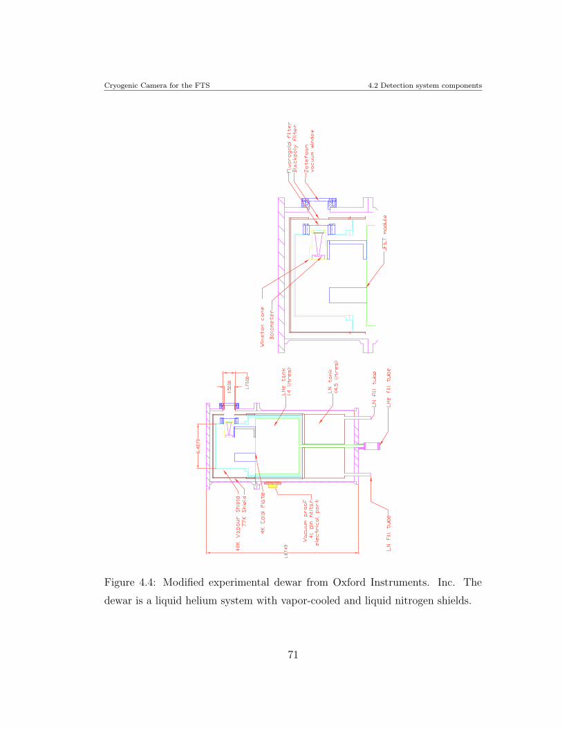
Cryogenic Camera for the FTS 4.2 Detection system components
Figure 4.4: Modified experimental dewar from Oxford Instruments. Inc. The
dewar is a liquid helium system with vapor-cooled and liquid nitrogen shields.
71
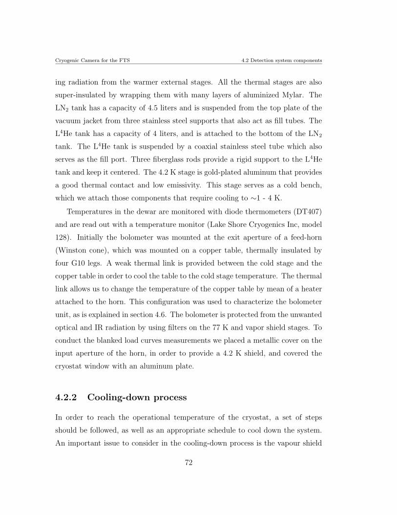
Cryogenic Camera for the FTS 4.2 Detection system components
ing radiation from the warmer external stages. All the thermal stages are also
super-insulated by wrapping them with many layers of aluminized Mylar. The
LN2 tank has a capacity of 4.5 liters and is suspended from the top plate of the
vacuum jacket from three stainless steel supports that also act as fill tubes. The
L4He tank has a capacity of 4 liters, and is attached to the bottom of the LN2
tank. The L4He tank is suspended by a coaxial stainless steel tube which also
serves as the fill port. Three fiberglass rods provide a rigid support to the L4He
tank and keep it centered. The 4.2 K stage is gold-plated aluminum that provides
a good thermal contact and low emissivity. This stage serves as a cold bench,
which we attach those components that require cooling to ∼1 - 4 K.
Temperatures in the dewar are monitored with diode thermometers (DT407)
and are read out with a temperature monitor (Lake Shore Cryogenics Inc, model
128). Initially the bolometer was mounted at the exit aperture of a feed-horn
(Winston cone), which was mounted on a copper table, thermally insulated by
four G10 legs. A weak thermal link is provided between the cold stage and the
copper table in order to cool the table to the cold stage temperature. The thermal
link allows us to change the temperature of the copper table by mean of a heater
attached to the horn. This configuration was used to characterize the bolometer
unit, as is explained in section 4.6. The bolometer is protected from the unwanted
optical and IR radiation by using filters on the 77 K and vapor shield stages. To
conduct the blanked load curves measurements we placed a metallic cover on the
input aperture of the horn, in order to provide a 4.2 K shield, and covered the
cryostat window with an aluminum plate.
4.2.2 Cooling-down process
In order to reach the operational temperature of the cryostat, a set of steps
should be followed, as well as an appropriate schedule to cool down the system.
An important issue to consider in the cooling-down process is the vapour shield
72
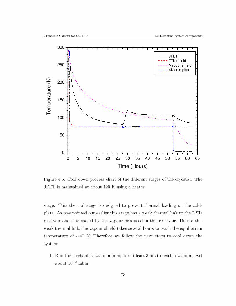
Cryogenic Camera for the FTS 4.2 Detection system components
0 5 10 15 20 25 30 35 40 45 50 55 60 650
50
100
150
200
250
300
Tem
pera
ture
(K)
Time (Hours)
JFET 77K shield Vapour shield 4K cold plate
Figure 4.5: Cool down process chart of the different stages of the cryostat. The
JFET is maintained at about 120 K using a heater.
stage. This thermal stage is designed to prevent thermal loading on the cold-
plate. As was pointed out earlier this stage has a weak thermal link to the L4He
reservoir and it is cooled by the vapour produced in this reservoir. Due to this
weak thermal link, the vapour shield takes several hours to reach the equilibrium
temperature of ∼40 K. Therefore we follow the next steps to cool down the
system:
1. Run the mechanical vacuum pump for at least 3 hrs to reach a vacuum level
about 10−2 mbar.
73
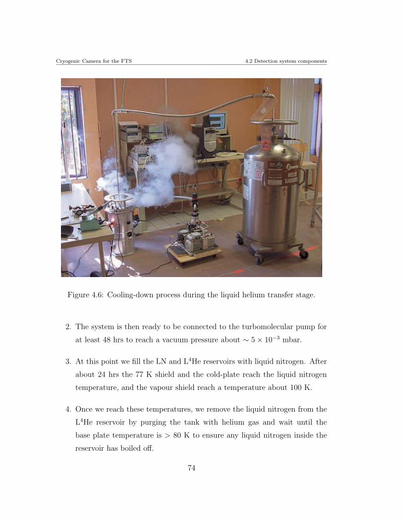
Cryogenic Camera for the FTS 4.2 Detection system components
Figure 4.6: Cooling-down process during the liquid helium transfer stage.
2. The system is then ready to be connected to the turbomolecular pump for
at least 48 hrs to reach a vacuum pressure about ∼ 5 × 10⁻³ mbar.
3. At this point we fill the LN and L4He reservoirs with liquid nitrogen. After
about 24 hrs the 77 K shield and the cold-plate reach the liquid nitrogen
temperature, and the vapour shield reach a temperature about 100 K.
4. Once we reach these temperatures, we remove the liquid nitrogen from the
L4He reservoir by purging the tank with helium gas and wait until the
base plate temperature is > 80 K to ensure any liquid nitrogen inside the
reservoir has boiled off.
74
Cryogenic Camera for the FTS 4.2 Detection system components
5. The liquid helium transfer is performed. The cooling-down takes about 18
to 20 hrs to reach a temperature of ∼3.9 K (boil-off temperature at 2200
m local altitude).
6. In case of a 1.8 K operational temperature we start pumping on the L4He
reservoir with the mechanical pump. The process takes ∼2 hrs.
The complete the cold-down process takes approximately 4 days to be ready
for any experiment. Figure 4.5 shows the typical curve for the various steps
involved in cooling-down process. Figure 4.6 shows a view of the laboratory
during the liquid helium transfer.
4.2.3 Temperature stability at the cold-plate
When the system is working at 3.9 K the temperature of the base-plate is stable,
however we have had a problem with the temperature stability at the detector.
The figure 4.4 shows the mechanical drawing of the internal configuration and the
position of the internal electronics on the baseplate. The bolometer is mounted
at the back of the Winston cone, which is placed on a copper table close to the
vapour shield. We identified that even with a good IR-blocking filtering there
is a temperature gradient of ∼70 mK between the feed-horn and the base plate,
which result in a strong dependence of the working temperature on the external
power loading conditions. In order to solve this drawback we modified the cold
optics.
The goal of the modification was to have a stable temperature across the
body of the feed-horn and define a new field of view for coupling with the FTS-
MPI. Greater thermal stability was achieved by placing the field optics directly
to the cold plate. The original f/2.4 Winston cone however is not suitable for
this option because the large acceptance angle (i.e. ∼ 22 degrees). Hence we
designed a new feed-horn with smaller acceptance angle (∼12 degrees) than the
75
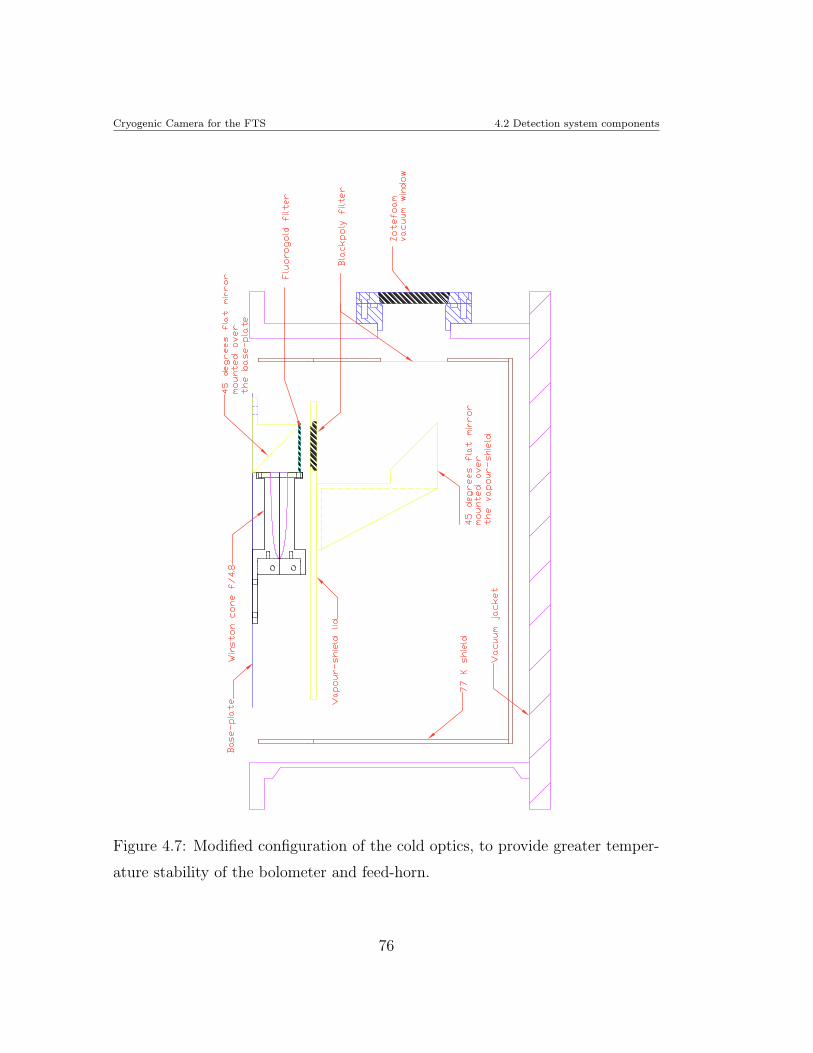
Cryogenic Camera for the FTS 4.2 Detection system components
Figure 4.7: Modified configuration of the cold optics, to provide greater temper-
ature stability of the bolometer and feed-horn.
76
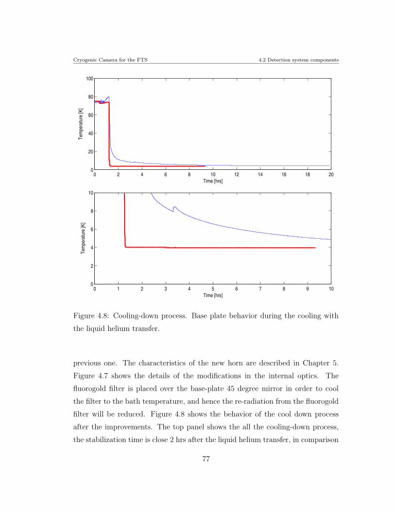
Cryogenic Camera for the FTS 4.2 Detection system components
0 2 4 6 8 10 12 14 16 18 200
20
40
60
80
100
Time [hrs]
Tem
pera
ture
[K]
0 1 2 3 4 5 6 7 8 9 100
2
4
6
8
10
Time [hrs]
Tem
pera
ture
[K]
Figure 4.8: Cooling-down process. Base plate behavior during the cooling with
the liquid helium transfer.
previous one. The characteristics of the new horn are described in Chapter 5.
Figure 4.7 shows the details of the modifications in the internal optics. The
fluorogold filter is placed over the base-plate 45 degree mirror in order to cool
the filter to the bath temperature, and hence the re-radiation from the fluorogold
filter will be reduced. Figure 4.8 shows the behavior of the cool down process
after the improvements. The top panel shows the all the cooling-down process,
the stabilization time is close 2 hrs after the liquid helium transfer, in comparison
77
Cryogenic Camera for the FTS 4.2 Detection system components
with the old configuration that takes close to 12 hrs to be stable (see Fig. 4.5).
4.2.4 Read-out electronics
Figure 4.9 shows the basic scheme for the biasing and the readout of the sensor.
The bolometer is biased with two 10 MΩ load resistors, RL, in series. The resistor
chain is symmetric in order to provide differential measurements. The bolometer
is mounted at the exit aperture of the feed-horn and the load resistances package
are screwed at the back of the horn on a small PCB circuit. In order to improve
the power absorption of the bolometer we installed an aluminum plate to act as a
back-short. The back-short also will allow better thermal conduction between the
feed-horn and the load resistor package. The load resistor unit is at or close to the
bath temperature in order to minimize its contribution to the Johnson noise and
it is physically close to the bolometer unit in order to minimize the microphonic
noise. The bolometer is connected to the high impedance pre-amplifier stage,
which is a coupled pair SST/U401 JFET transistor configured in a differential
follower mode in order to have high noise rejection.
The noise density contribution reported by the manufacturer is ∼5 nV/Hz1/2.
The JFET pre-amplifier is mounted on the cold stage (∼ 4.2 K), but is thermally
isolated by a G10 tube. The working JFET temperature (∼ 120 K) is achieved by
mean of a heater attached directly to the JFET module. The JFET pre-amplifier
stage is also placed close to the bolometer unit in order to reduce the length of the
connection wires and hence reduce microphonic pick-up through the wires. The
detector is connected to the pre-amplifier stage with twisted pair of manganin
wires in order to null the magnetic interference and these twisted pair were made
as short as possible and held in place with Stycast 2850. The next stage is an
amplification system (at room temperature), which provides a gain to the output
signal coming from the JFET module. The amplifier uses an instrumentation
amplifier AD624AD from Analog Devices, designed to have both AC and DC
78

Cryogenic Camera for the FTS 4.2 Detection system components
+Vbias
-Vbias
+Vdd
-Vss
10 MΩΩΩΩ
10 MΩΩΩΩ
BolometerJFET
module
~ 120 K
~ 4.2 K
Room temperature
Warm amplifier
Figure 4.9: The bolometer schematic circuit for biasing and readout. The gray
boxes show the different temperature stages.
outputs. The AC stage provides a differential output with selectable gains (i.e.
1, 2, 5 and 10). The AC output pass through an active bi-quad bandpass filter,
designed to provided an additional gain of ∼ 2.5.
The signal from the second amplification stage is then digitized by a digital
acquisition (DAQ) system from National Instruments. The PCI-6024E DAQ is a
200 Ks/s, 12-bit system, that allows us to have 16 single-end and 8 differential
analog inputs. The DAQ system is fully supported by the graphical program
LabView, which we used to develop our graphical interface for control and data
acquisition. A brief description of the acquisition and control software will be
given in section 4.2.7.
79
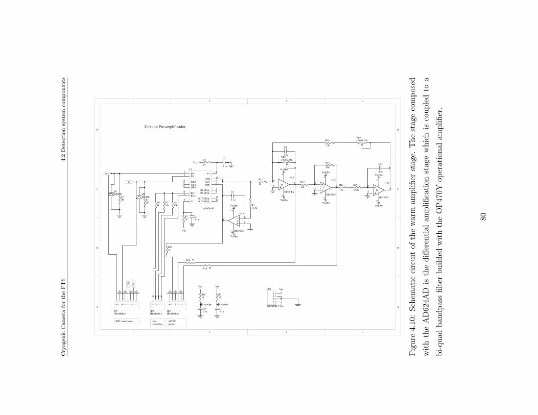
Cry
ogen
icC
am
era
for
the
FT
S4.2
Det
ection
syst
emco
mponen
ts
1 2 3 4
A
B
C
D
4321
D
C
B
A
VccOps
VeeOps
R11
1k
VccOps
R13
10k
C4
4.7u
R12
10k
VeeOpsVeeOps
VccOps
R14
12k
C5
4.7u
7.5k
C2
0.1u
C10.1u
R310
R4
10
Vee
Vcc
R516.2k
VccOps
VeeOps
C3
4.7u
R1010
R910
C60.1u
C70.1u
Vcc Vee
VccOps VeeOps
2
31
411
A
U1A
OP470EY
5
67
411
B
U1B
OP470EY
9
108
114
C
U1C
OP470EY
13
1214
114
D
U1D
OP470EY
IN-1 IN+2
RG23
IN NULL 4
IN NULL 5
REF 6
V-7
V+ 8
OUT 9SEN 10
G50011 G20012 G10013
OUT NULL 14OUT NULL 15
RG116
U2
AD624AD
R21M R1
1M
R15
3.92k
R18 10
R19 10
R171k
Circuito Pre-amplificador
R710k
R840k
R64k
Vd1
Vd2
Vs+
Vs-
1234
JP2
HEADER 4
Vcc
Vee
12345678
JP1HEADER 8
1234
JP3HEADER 4
123456
JP4HEADER 6
JFET connections Gainconnections
AC/DCoutputs
D1DIODE D2
DIODE
Fig
ure
4.10
:Sch
emat
icci
rcuit
ofth
ew
arm
amplifier
stag
e.T
he
stag
eco
mpos
ed
with
the
AD
624A
Dis
the
diff
eren
tial
amplifica
tion
stag
ew
hic
his
couple
dto
a
bi-quad
ban
dpas
sfilter
builded
with
the
OP
470Y
oper
atio
nal
amplifier
.
80
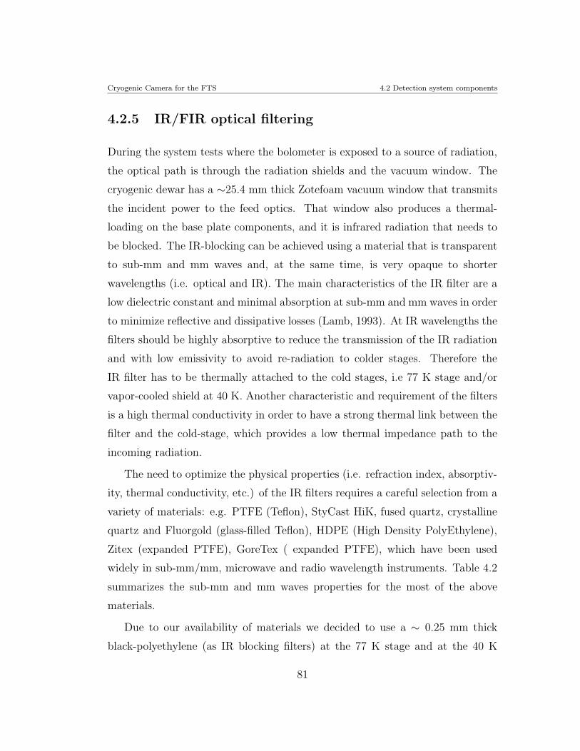
Cryogenic Camera for the FTS 4.2 Detection system components
4.2.5 IR/FIR optical filtering
During the system tests where the bolometer is exposed to a source of radiation,
the optical path is through the radiation shields and the vacuum window. The
cryogenic dewar has a ∼25.4 mm thick Zotefoam vacuum window that transmits
the incident power to the feed optics. That window also produces a thermal-
loading on the base plate components, and it is infrared radiation that needs to
be blocked. The IR-blocking can be achieved using a material that is transparent
to sub-mm and mm waves and, at the same time, is very opaque to shorter
wavelengths (i.e. optical and IR). The main characteristics of the IR filter are a
low dielectric constant and minimal absorption at sub-mm and mm waves in order
to minimize reflective and dissipative losses (Lamb, 1993). At IR wavelengths the
filters should be highly absorptive to reduce the transmission of the IR radiation
and with low emissivity to avoid re-radiation to colder stages. Therefore the
IR filter has to be thermally attached to the cold stages, i.e 77 K stage and/or
vapor-cooled shield at 40 K. Another characteristic and requirement of the filters
is a high thermal conductivity in order to have a strong thermal link between the
filter and the cold-stage, which provides a low thermal impedance path to the
incoming radiation.
The need to optimize the physical properties (i.e. refraction index, absorptiv-
ity, thermal conductivity, etc.) of the IR filters requires a careful selection from a
variety of materials: e.g. PTFE (Teflon), StyCast HiK, fused quartz, crystalline
quartz and Fluorgold (glass-filled Teflon), HDPE (High Density PolyEthylene),
Zitex (expanded PTFE), GoreTex ( expanded PTFE), which have been used
widely in sub-mm/mm, microwave and radio wavelength instruments. Table 4.2
summarizes the sub-mm and mm waves properties for the most of the above
materials.
Due to our availability of materials we decided to use a ∼ 0.25 mm thick
black-polyethylene (as IR blocking filters) at the 77 K stage and at the 40 K
81
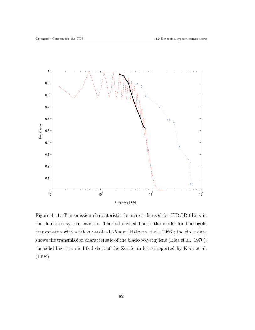
Cryogenic Camera for the FTS 4.2 Detection system components
101
102
103
104
0
0.1
0.2
0.3
0.4
0.5
0.6
0.7
0.8
0.9
1
Frequency [GHz]
Tran
smiss
ion
Figure 4.11: Transmission characteristic for materials used for FIR/IR filters in
the detection system camera. The red-dashed line is the model for fluorogold
transmission with a thickness of ∼1.25 mm (Halpern et al., 1986); the circle data
shows the transmission characteristic of the black-polyethylene (Blea et al., 1970);
the solid line is a modified data of the Zotefoam losses reported by Kooi et al.
(1998).
82
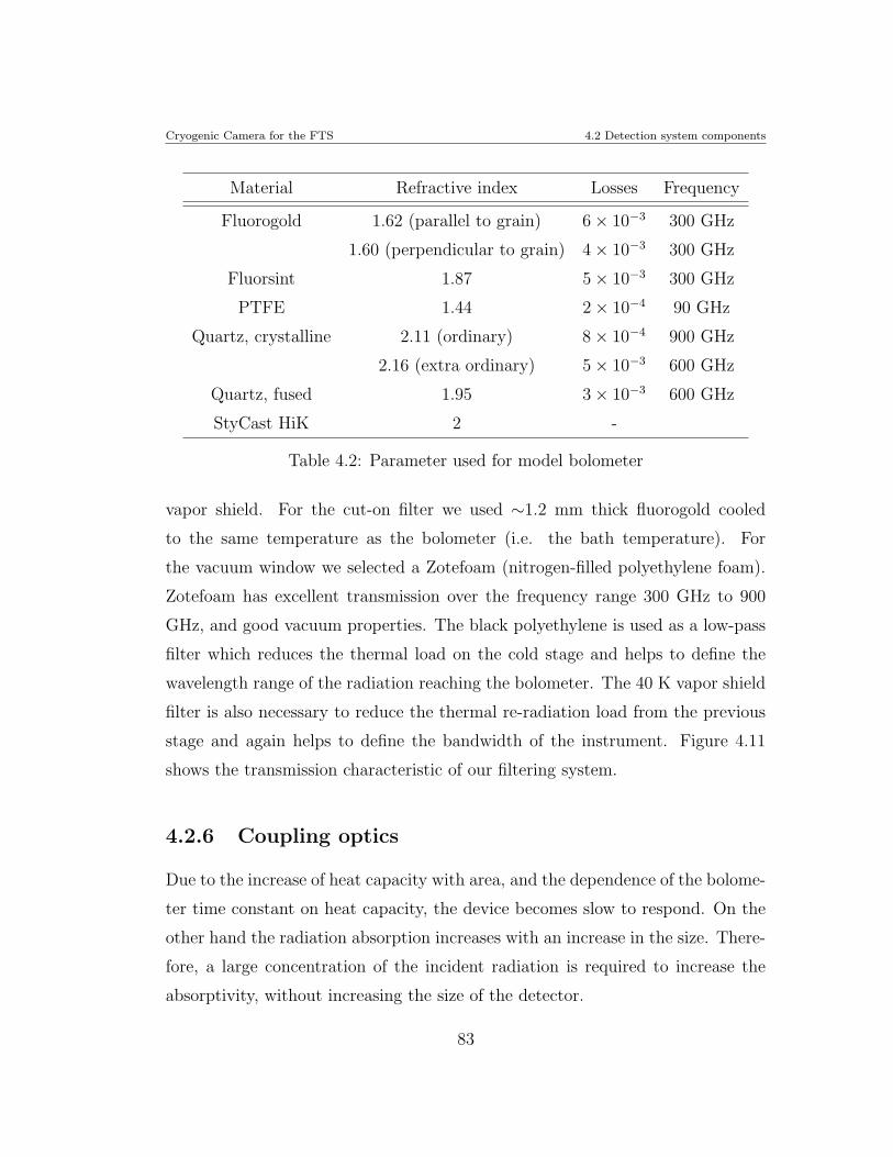
Cryogenic Camera for the FTS 4.2 Detection system components
Material Refractive index Losses Frequency
Fluorogold 1.62 (parallel to grain) 6 × 10⁻³ 300 GHz
1.60 (perpendicular to grain) 4 × 10⁻³ 300 GHz
Fluorsint 1.87 5 × 10⁻³ 300 GHz
PTFE 1.44 2 × 10⁻⁴ 90 GHz
Quartz, crystalline 2.11 (ordinary) 8 × 10⁻⁴ 900 GHz
2.16 (extra ordinary) 5 × 10⁻³ 600 GHz
Quartz, fused 1.95 3 × 10⁻³ 600 GHz
StyCast HiK 2 -
Table 4.2: Parameter used for model bolometer
vapor shield. For the cut-on filter we used ∼1.2 mm thick fluorogold cooled
to the same temperature as the bolometer (i.e. the bath temperature). For
the vacuum window we selected a Zotefoam (nitrogen-filled polyethylene foam).
Zotefoam has excellent transmission over the frequency range 300 GHz to 900
GHz, and good vacuum properties. The black polyethylene is used as a low-pass
filter which reduces the thermal load on the cold stage and helps to define the
wavelength range of the radiation reaching the bolometer. The 40 K vapor shield
filter is also necessary to reduce the thermal re-radiation load from the previous
stage and again helps to define the bandwidth of the instrument. Figure 4.11
shows the transmission characteristic of our filtering system.
4.2.6 Coupling optics
Due to the increase of heat capacity with area, and the dependence of the bolome-
ter time constant on heat capacity, the device becomes slow to respond. On the
other hand the radiation absorption increases with an increase in the size. There-
fore, a large concentration of the incident radiation is required to increase the
absorptivity, without increasing the size of the detector.
83
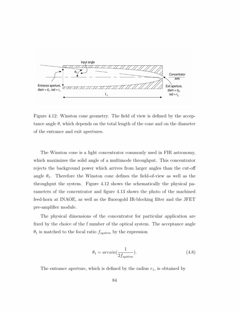
Cryogenic Camera for the FTS 4.2 Detection system components
Exit aperture, diam = d2, rad = r2.
Entrance aperture, diam = d1, rad = r1.
θ1
Input angle
l L
Concentratoraxis
Figure 4.12: Winston cone geometry. The field of view is defined by the accep-
tance angle θ, which depends on the total length of the cone and on the diameter
of the entrance and exit apertures.
The Winston cone is a light concentrator commonly used in FIR astronomy,
which maximizes the solid angle of a multimode throughput. This concentrator
rejects the background power which arrives from larger angles than the cut-off
angle θ1. Therefore the Winston cone defines the field-of-view as well as the
throughput the system. Figure 4.12 shows the schematically the physical pa-
rameters of the concentrator and figure 4.13 shows the photo of the machined
feed-horn at INAOE, as well as the fluorogold IR-blocking filter and the JFET
pre-amplifier module.
The physical dimensions of the concentrator for particular application are
fixed by the choice of the f number of the optical system. The acceptance angle
θ1 is matched to the focal ratio fsystem by the expression
θ1 = arcsin(1
2fsystem
). (4.8)
The entrance aperture, which is defined by the radius r1, is obtained by
84
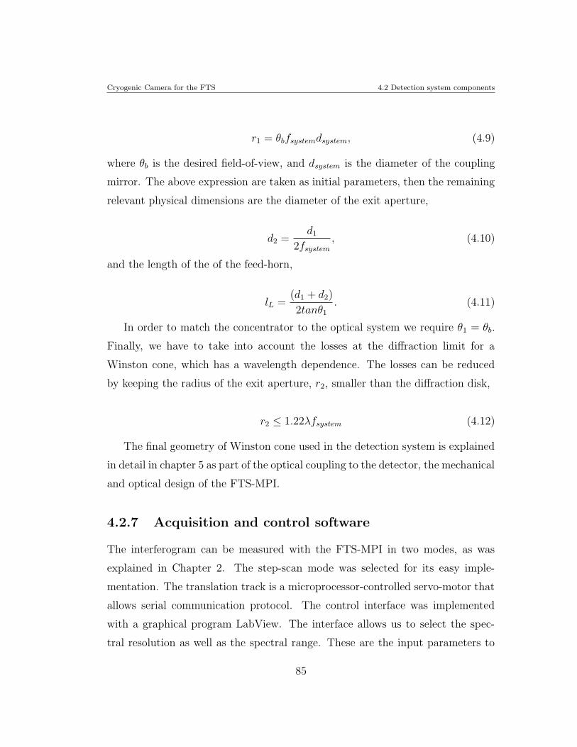
Cryogenic Camera for the FTS 4.2 Detection system components
r1 = θbfsystemdsystem, (4.9)
where θb is the desired field-of-view, and dsystem is the diameter of the coupling
mirror. The above expression are taken as initial parameters, then the remaining
relevant physical dimensions are the diameter of the exit aperture,
d2 =d1
2fsystem
, (4.10)
and the length of the of the feed-horn,
lL =(d1 + d2)
2tanθ1
. (4.11)
In order to match the concentrator to the optical system we require θ1 = θb.
Finally, we have to take into account the losses at the diffraction limit for a
Winston cone, which has a wavelength dependence. The losses can be reduced
by keeping the radius of the exit aperture, r2, smaller than the diffraction disk,
r2 ≤ 1.22λfsystem (4.12)
The final geometry of Winston cone used in the detection system is explained
in detail in chapter 5 as part of the optical coupling to the detector, the mechanical
and optical design of the FTS-MPI.
4.2.7 Acquisition and control software
The interferogram can be measured with the FTS-MPI in two modes, as was
explained in Chapter 2. The step-scan mode was selected for its easy imple-
mentation. The translation track is a microprocessor-controlled servo-motor that
allows serial communication protocol. The control interface was implemented
with a graphical program LabView. The interface allows us to select the spec-
tral resolution as well as the spectral range. These are the input parameters to
85
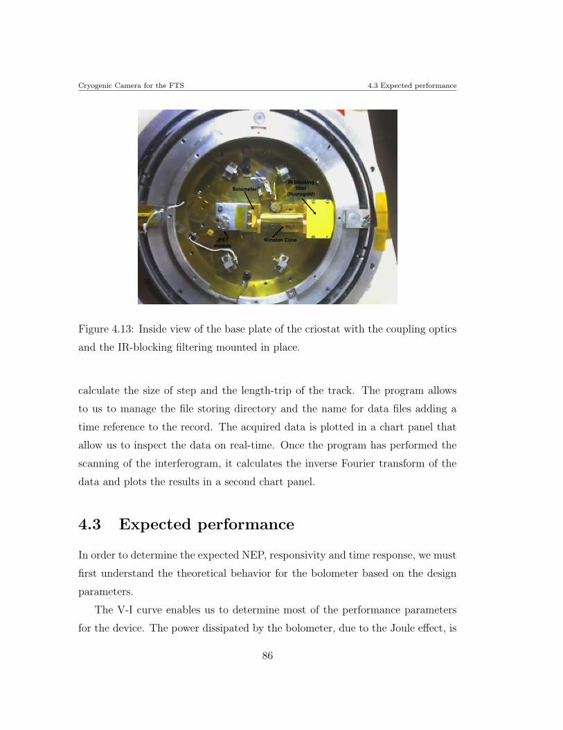
Cryogenic Camera for the FTS 4.3 Expected performance
Winston Cone
Bolometer
JFET module
IR blockingfilter
(fluorogold)
Figure 4.13: Inside view of the base plate of the criostat with the coupling optics
and the IR-blocking filtering mounted in place.
calculate the size of step and the length-trip of the track. The program allows
to us to manage the file storing directory and the name for data files adding a
time reference to the record. The acquired data is plotted in a chart panel that
allow us to inspect the data on real-time. Once the program has performed the
scanning of the interferogram, it calculates the inverse Fourier transform of the
data and plots the results in a second chart panel.
4.3 Expected performance
In order to determine the expected NEP, responsivity and time response, we must
first understand the theoretical behavior for the bolometer based on the design
parameters.
The V-I curve enables us to determine most of the performance parameters
for the device. The power dissipated by the bolometer, due to the Joule effect, is
86
Cryogenic Camera for the FTS 4.3 Expected performance
P = I2biasRbol = VbolIbias
and so, Ibias =√
P/Rbol, or Vbol =√
P · Rbol
(4.13)
The rate of heat flow out of the bolometer W ,
W = Pbias + Q, (4.14)
where Pbias is the power dissipated by the bolometer due to the bias current, and
Q is the incident power. On the other hand, we know that in a steady state
condition the thermal conductance G0 depends on the bath temperature. The
heat flow W passing through the thermal link is equal to the thermal conductance
times the temperature gradient through the thermal link,
W = G0 · (T − T0) (4.15)
The dynamic thermal conductance Gd, which measures the change in the rate
of heat flow W , caused by a change in the temperature T , is derived by taking
the derivative of Eq. 4.14. In the case of a constant incident power we have,
Gd =dW
dT=
dPbias
dT(4.16)
Using Eq. 4.16 and 4.14, we get the power dissipated by the bolometer,
Pbias =
∫ T
T0
GddT − Q (4.17)
Now, from Fig 4.3, we know that the thermal conductivity could be described
by the power-law G0(T/T0)β and hence we can calculate the electrical power
dissipated as follows,
Pbias = G0
(
T
T0
)β
(T − T0) − Q (4.18)
Using Eq. 4.18 we calculate the bias current and bolometer voltage as function
of the temperature change of the bolometer. For a given set of parameters (β,
87
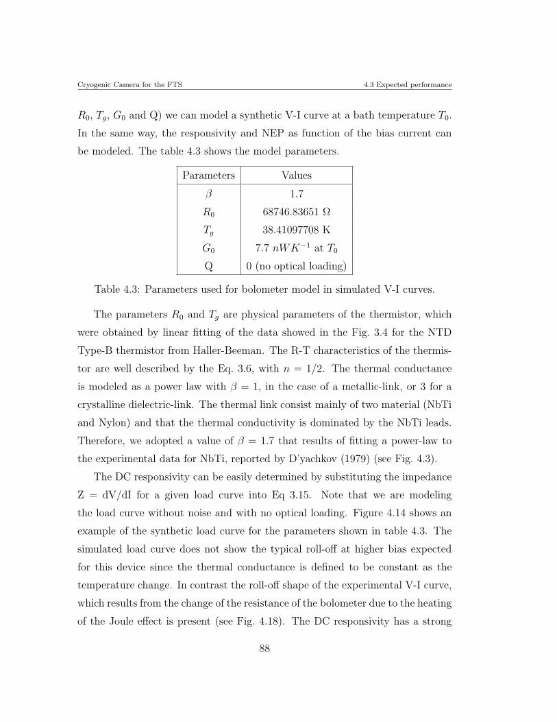
Cryogenic Camera for the FTS 4.3 Expected performance
R0, Tg, G0 and Q) we can model a synthetic V-I curve at a bath temperature T0.
In the same way, the responsivity and NEP as function of the bias current can
be modeled. The table 4.3 shows the model parameters.
Parameters Values
β 1.7
R0 68746.83651 Ω
Tg 38.41097708 K
G0 7.7 nWK−1 at T0
Q 0 (no optical loading)
Table 4.3: Parameters used for bolometer model in simulated V-I curves.
The parameters R0 and Tg are physical parameters of the thermistor, which
were obtained by linear fitting of the data showed in the Fig. 3.4 for the NTD
Type-B thermistor from Haller-Beeman. The R-T characteristics of the thermis-
tor are well described by the Eq. 3.6, with n = 1/2. The thermal conductance
is modeled as a power law with β = 1, in the case of a metallic-link, or 3 for a
crystalline dielectric-link. The thermal link consist mainly of two material (NbTi
and Nylon) and that the thermal conductivity is dominated by the NbTi leads.
Therefore, we adopted a value of β = 1.7 that results of fitting a power-law to
the experimental data for NbTi, reported by D’yachkov (1979) (see Fig. 4.3).
The DC responsivity can be easily determined by substituting the impedance
Z = dV/dI for a given load curve into Eq 3.15. Note that we are modeling
the load curve without noise and with no optical loading. Figure 4.14 shows an
example of the synthetic load curve for the parameters shown in table 4.3. The
simulated load curve does not show the typical roll-off at higher bias expected
for this device since the thermal conductance is defined to be constant as the
temperature change. In contrast the roll-off shape of the experimental V-I curve,
which results from the change of the resistance of the bolometer due to the heating
of the Joule effect is present (see Fig. 4.18). The DC responsivity has a strong
88
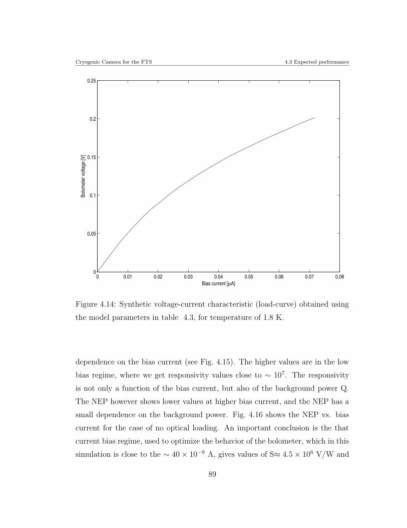
Cryogenic Camera for the FTS 4.3 Expected performance
0 0.01 0.02 0.03 0.04 0.05 0.06 0.07 0.080
0.05
0.1
0.15
0.2
0.25 B
olom
eter
vol
tage
[V]
Bias current [µA]
Figure 4.14: Synthetic voltage-current characteristic (load-curve) obtained using
the model parameters in table 4.3, for temperature of 1.8 K.
dependence on the bias current (see Fig. 4.15). The higher values are in the low
bias regime, where we get responsivity values close to ∼ 107. The responsivity
is not only a function of the bias current, but also of the background power Q.
The NEP however shows lower values at higher bias current, and the NEP has a
small dependence on the background power. Fig. 4.16 shows the NEP vs. bias
current for the case of no optical loading. An important conclusion is the that
current bias regime, used to optimize the behavior of the bolometer, which in this
simulation is close to the ∼ 40 × 10−9 A, gives values of S≈ 4.5 × 10⁶ V/W and
89
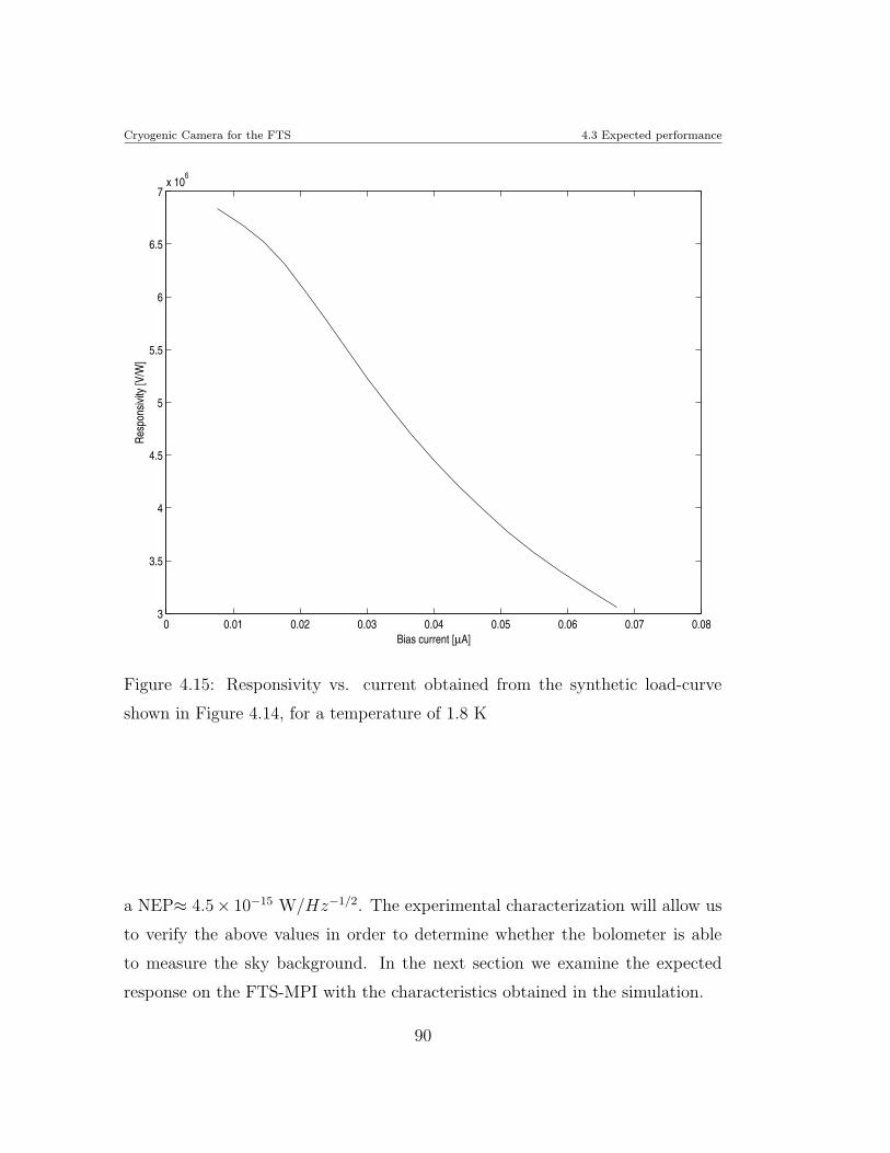
Cryogenic Camera for the FTS 4.3 Expected performance
0 0.01 0.02 0.03 0.04 0.05 0.06 0.07 0.083
3.5
4
4.5
5
5.5
6
6.5
7x 10
6
Res
pons
ivity
[V/W
]
Bias current [µA]
Figure 4.15: Responsivity vs. current obtained from the synthetic load-curve
shown in Figure 4.14, for a temperature of 1.8 K
a NEP≈ 4.5× 10⁻¹⁵ W/Hz−1/2. The experimental characterization will allow us
to verify the above values in order to determine whether the bolometer is able
to measure the sky background. In the next section we examine the expected
response on the FTS-MPI with the characteristics obtained in the simulation.
90
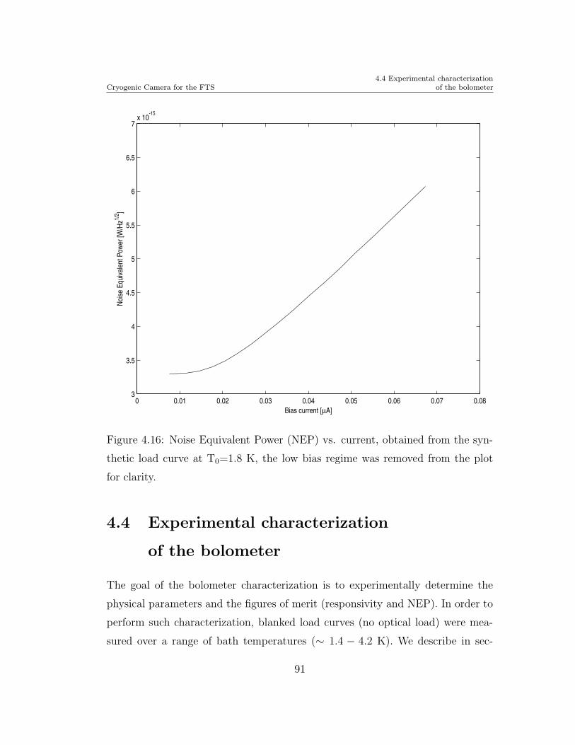
Cryogenic Camera for the FTS4.4 Experimental characterization
of the bolometer
0 0.01 0.02 0.03 0.04 0.05 0.06 0.07 0.083
3.5
4
4.5
5
5.5
6
6.5
7x 10
-15 N
oise
Equ
ivale
nt P
ower
[W/H
z1/2 ]
Bias current [µA]
Figure 4.16: Noise Equivalent Power (NEP) vs. current, obtained from the syn-
thetic load curve at T0=1.8 K, the low bias regime was removed from the plot
for clarity.
4.4 Experimental characterization
of the bolometer
The goal of the bolometer characterization is to experimentally determine the
physical parameters and the figures of merit (responsivity and NEP). In order to
perform such characterization, blanked load curves (no optical load) were mea-
sured over a range of bath temperatures (∼ 1.4 − 4.2 K). We describe in sec-
91
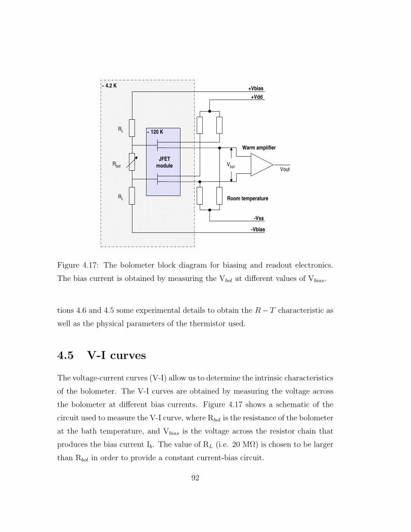
Cryogenic Camera for the FTS 4.5 V-I curves
+Vbias
-Vbias
+Vdd
-Vss
RL
RL
Rbol
JFET module
~ 120 K
~ 4.2 K
Room temperature
Warm amplifier
Vbol Vout
Figure 4.17: The bolometer block diagram for biasing and readout electronics.
The bias current is obtained by measuring the Vbol at different values of Vbias.
tions 4.6 and 4.5 some experimental details to obtain the R− T characteristic as
well as the physical parameters of the thermistor used.
4.5 V-I curves
The voltage-current curves (V-I) allow us to determine the intrinsic characteristics
of the bolometer. The V-I curves are obtained by measuring the voltage across
the bolometer at different bias currents. Figure 4.17 shows a schematic of the
circuit used to measure the V-I curve, where Rbol is the resistance of the bolometer
at the bath temperature, and Vbias is the voltage across the resistor chain that
produces the bias current Ib. The value of RL (i.e. 20 MΩ) is chosen to be larger
than Rbol in order to provide a constant current-bias circuit.
92
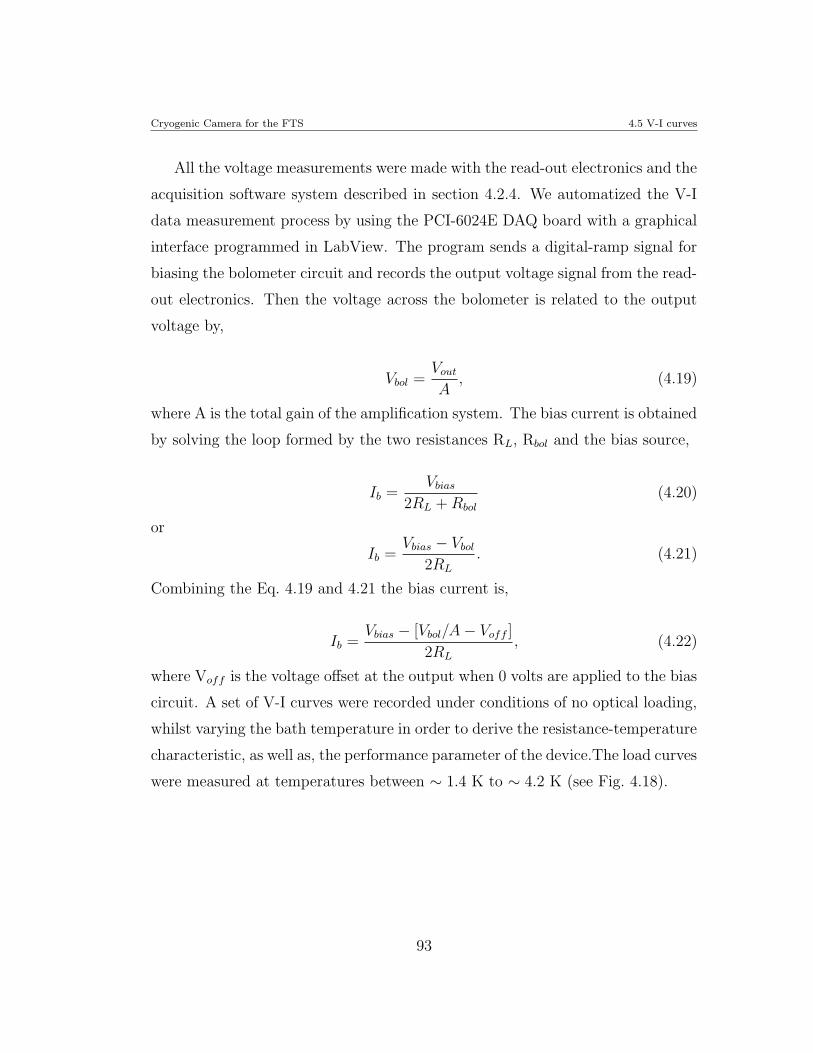
Cryogenic Camera for the FTS 4.5 V-I curves
All the voltage measurements were made with the read-out electronics and the
acquisition software system described in section 4.2.4. We automatized the V-I
data measurement process by using the PCI-6024E DAQ board with a graphical
interface programmed in LabView. The program sends a digital-ramp signal for
biasing the bolometer circuit and records the output voltage signal from the read-
out electronics. Then the voltage across the bolometer is related to the output
voltage by,
Vbol =Vout
A, (4.19)
where A is the total gain of the amplification system. The bias current is obtained
by solving the loop formed by the two resistances RL, Rbol and the bias source,
Ib =Vbias
2RL + Rbol
(4.20)
or
Ib =Vbias − Vbol
2RL
. (4.21)
Combining the Eq. 4.19 and 4.21 the bias current is,
Ib =Vbias − [Vbol/A − Voff ]
2RL
, (4.22)
where Voff is the voltage offset at the output when 0 volts are applied to the bias
circuit. A set of V-I curves were recorded under conditions of no optical loading,
whilst varying the bath temperature in order to derive the resistance-temperature
characteristic, as well as, the performance parameter of the device.The load curves
were measured at temperatures between ∼ 1.4 K to ∼ 4.2 K (see Fig. 4.18).
93
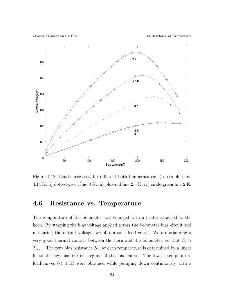
Cryogenic Camera for the FTS 4.6 Resistance vs. Temperature
50 100 150 200 250 3000
0.1
0.2
0.3
0.4
0.5
0.6
Bias current [nA]
Bolo
met
er v
olta
ge [V
]
4.14K
3 K
2 K
2.5 K
Figure 4.18: Load-curves set, for different bath temperatures: i) cross-blue line
4.14 K; ii) dotted-green line 3 K; iii) plus-red line 2.5 K; iv) circle-green line 2 K.
4.6 Resistance vs. Temperature
The temperature of the bolometer was changed with a heater attached to the
horn. By stepping the bias voltage applied across the bolometer bias circuit and
measuring the output voltage, we obtain each load curve. We are assuming a
very good thermal contact between the horn and the bolometer, so that Tb ≈Thorn. The zero bias resistance R0, at each temperature is determined by a linear
fit to the low bias current regime of the load curve. The lowest temperature
load-curves (< 4 K) were obtained while pumping down continuously with a
94
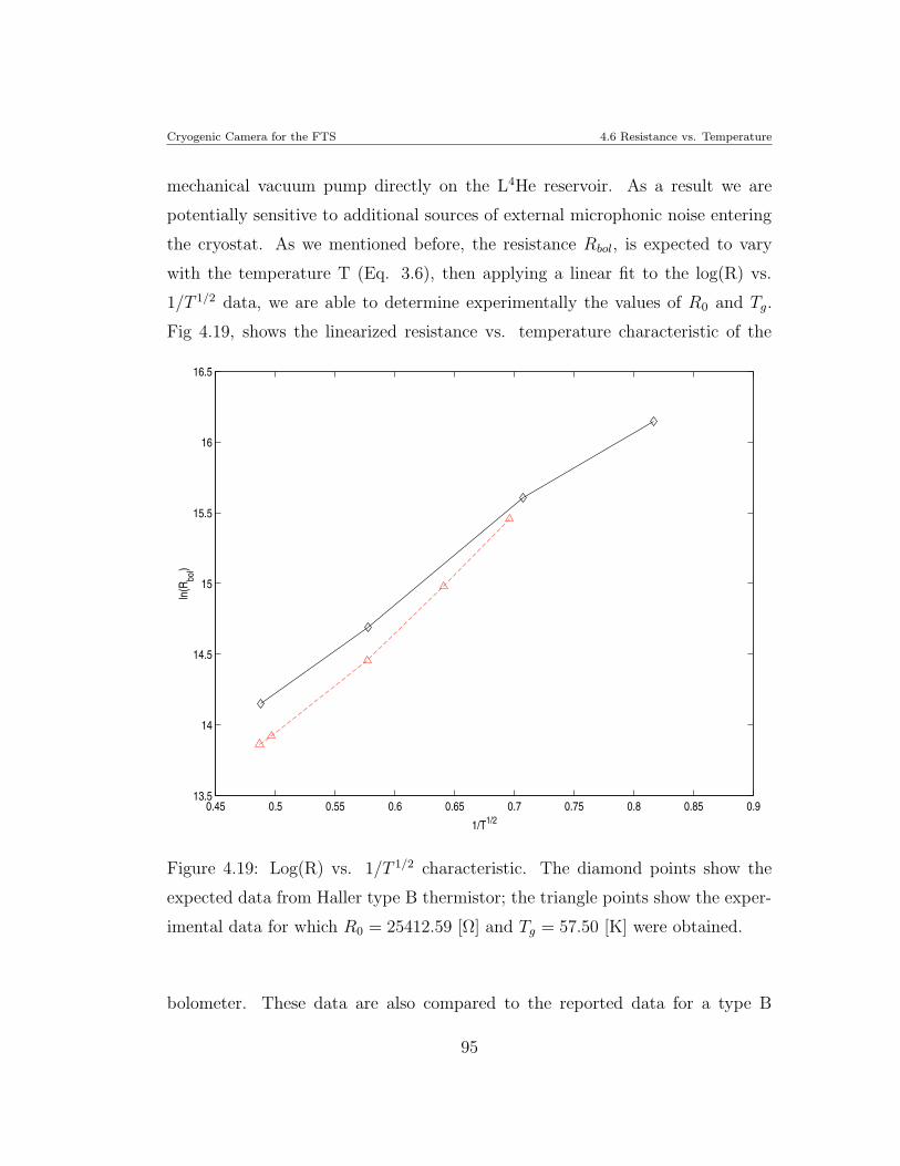
Cryogenic Camera for the FTS 4.6 Resistance vs. Temperature
mechanical vacuum pump directly on the L4He reservoir. As a result we are
potentially sensitive to additional sources of external microphonic noise entering
the cryostat. As we mentioned before, the resistance Rbol, is expected to vary
with the temperature T (Eq. 3.6), then applying a linear fit to the log(R) vs.
1/T 1/2 data, we are able to determine experimentally the values of R0 and Tg.
Fig 4.19, shows the linearized resistance vs. temperature characteristic of the
0.45 0.5 0.55 0.6 0.65 0.7 0.75 0.8 0.85 0.913.5
14
14.5
15
15.5
16
16.5
1/T1/2
ln(R
bol)
Figure 4.19: Log(R) vs. 1/T 1/2 characteristic. The diamond points show the
expected data from Haller type B thermistor; the triangle points show the exper-
imental data for which R0 = 25412.59 [Ω] and Tg = 57.50 [K] were obtained.
bolometer. These data are also compared to the reported data for a type B
95
Cryogenic Camera for the FTS 4.7 Electrical responsivity
thermistor from Haller-Beeman. The differences between the experimental data
and Haller-Beeman data are still consistent within the errors in the measurements.
The device does not show any significant heating from IR radiation leakages or
thermal conduction leakages due to the wiring. Thus from the experimental data
we obtained values of R0 = 25412.59 [Ω] and Tg = 57.50 [K]. That does not affect
the performance of the bolometer because the resistive coefficient is consistent
with that obtained with the reported data.
4.7 Electrical responsivity
It is very important to establish the operating point of the detector in order to
maximize the responsivity. The maximum responsivity is achieved for a value of Z
≈ 0, where the responsivity is S(0) = −1/2I. From the experiment measurements
at ∼ 1.9 K and ∼ 4.1 K, we showed that the responsivity has a monotonically
behavior.Fig 4.20 shows the responsivity versus bias-current at bath temperatures
of ∼ 4.1 K and ∼ 1.9 K. The responsivity at Ibias ∼ 40 nA for a temperature of
∼ 4.05 K is ∼ 1.4×10⁷ V/W, and for a temperature of ∼ 1.9 K we derive ∼ 1.75×10⁷ V/W which represents just as small responsivity increment, that is because
the results at ∼ 1.9 K were obtained pumping the L4He reservoir, that process
introduces noise due to large variations in the baseplate temperature. However
the experimental value of the responsivity is at least one order of magnitude larger
than that obtained by the simulation for about the same bias-current condition,
i.e for a bias-current of ∼40 nA is ∼ 4.5 × 10⁶ V/W.
4.8 Noise Equivalent Power
The measured NEP is related to the electrical and thermal noise contribution to
the system. In principle all the sources of noise should be lower than the thermal
noise, in order to achieve a background-limited system. From the blanked load
96
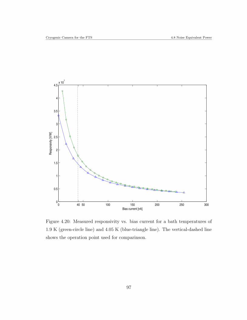
Cryogenic Camera for the FTS 4.8 Noise Equivalent Power
0 50 100 150 200 250 300400
0.5
1
1.5
2
2.5
3
3.5
4
4.5x 10
7
Bias current [nA]
Resp
onsiv
ity [V
/W]
Figure 4.20: Measured responsivity vs. bias current for a bath temperatures of
1.9 K (green-circle line) and 4.05 K (blue-triangle line). The vertical-dashed line
shows the operation point used for comparinson.
97
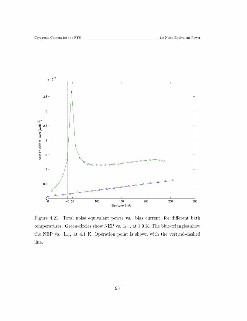
Cryogenic Camera for the FTS 4.8 Noise Equivalent Power
0 50 100 150 200 250 300400
0.5
1
1.5
2
2.5
3
3.5
x 10-14
Bias current [nA]
Noise
Equ
ivale
nt P
ower
[W/H
z1/2 ]
Figure 4.21: Total noise equivalent power vs. bias current, for different bath
temperatures. Green-circles show NEP vs. Ibias at 1.9 K. The blue-triangles show
the NEP vs. Ibias at 4.1 K. Operation point is shown with the vertical-dashed
line.
98
Cryogenic Camera for the FTS 4.9 The bolometric system on the FTS
curve at ∼ 4.2 K, we find an electrical (Johnson) noise excess, which degrades
the total NEP. Figure 4.21 shows the total NEP contribution of the system for
1.9 K and 4.1 K bath temperatures. The green-circle line shows a not typical
NEP curve, which is a clear effect of the bath temperature instability during the
measurements. However the NEP for those experimental temperatures are in the
order of ∼ 10−14 W/Hz1/2. Therefore it is clear that the best bath temperature
to operate the FTS-MPI system is at T0 ≈ 4.2 K due to the more stable behavior
of the system.
4.9 The bolometric system on the FTS
Finally we examine the behavior and suitability of the bolometer in the context of
acting as the cryogenic detector for the FTS-MPI. As was explained in chapter 3
if the bolometer is operating in a steady-state, the power falling on the bolometer
from a thermal source must equal the power dissipated through the thermal link
G0, which connects the bolometer unit to the heat sink (see equation 4.15).
In our case, that power, which the bolometer first measures, travels through
the interferometer. The FTS-MPI can be used in a two-input port configuration,
with one port looking at the source (e.g. room temperature baffles, the sky, etc.),
and the second port looking simultaneously at a polystyrene cup of liquid nitrogen
at ∼77 K, i.e. as a reference load. We can describe the power that reaches the
bolometer, as a function of the optical-path differences, δ, as
I(δ) =1
2(ILN + Isky) ±
1
2(ILN − Isky)cos(σδ). (4.23)
The first term represents the constant power which imposes a background on
the detector. The second term is the signal of the interest that is detected by
the readout electronics. The constant term in equation 4.23 is important because
it will affect the temperature at which the bolometer operates, and therefore
99
Cryogenic Camera for the FTS 4.9 The bolometric system on the FTS
its resistance. The second term which measures the difference between the two
sources also contains the required information to calculate the power spectrum.
In order to know the change in the temperature of the bolometer due to a
change in the incoming power we solve the equation 4.15 for temperature, i.e.
T =W
G0
+ T0 (4.24)
Therefore variations in the incoming power will produce a change in the re-
sistance of the bolometer. Using the R-T characteristic described by the Eq. 3.6
and the parameters used for modeling the theoretical behavior of the bolometer,
and using Eq. 4.24, we calculate ∆Rbol. Using the Haller-Beeman R-T curve, the
type B thermistor suggest a resistance-temperature ratio of ∆R∆T
≈ 0.98 MΩ/K.
Hence at T0 ≈ 4.2 K the expected value of ∆Rbol, when the interference term
shows the maximum contrast, is ∼ 1.5 MΩ. Therefore the bolometer has an
expected ∆R∆T
≈ 1 MΩ/K, which is in agreement with the thermistor chosen for
the bolometer design.
100
Chapter 5
FTS: System Design and
Integration
Fourier transform spectroscopy is a well established technique that is used in many
research areas such as gas spectroscopy, optical materials, etc. Due to its ability
to sample and study a wide frequency range, Fourier transform spectroscopy in
astronomy has also become an ideal tool for atmospheric site characterization at
sub-mm/mm wavelengths.
In Chapter 2, we have introduced the fundamentals in the analysis of data
(i.e. interferograms) taken with a Fourier transform spectrometer. In Chapters 3
and 4 the basic theory of bolometers and the fundamental blocks of the detection
system have been presented, as well as some details of the system integration and
characterization. In this chapter we shall describe details behind the selection
of the components integrated into our polarizing Martin-Puplett interferometer.
Results of the laboratory tests will also be shown and discussed, as well as the
analysis of synthetic spectra that allow us to evaluate the best strategy for the
data reduction, and which help to understand the performance of the real system.
101
FTS: System Design and Integration 5.1 Fourier transform spectrometer design
5.1 Fourier transform spectrometer design
A Martin-Puplett interferometer is a well-known configuration used in several
fields of spectroscopy. Our goal is to build an interferometer with the appropriate
characteristics to work in the areas of atmospheric spectroscopy, as well as optical
material characterization at sub-mm/mm wavelengths.
From the point of view of an ideal spectrometer, a high resolution and large
throughput system is desired. Large throughput will provide a good signal-to-
noise ratio, by collecting more radiation power from a larger solid-angle. On
the other hand, high resolution allow us to resolve fine spectral features. We
should be careful to understand the final application however, in order to avoid
unnecessary financial costs for the final system.
5.1.1 Spectral Resolution
We define spectral resolution by the frequency width that allows us to separate
two spectral lines. Generally it is defined in terms of the maximum optical path
difference δ. In practice we have to decide on a resolution that allows us to recover
the profile of the atmospheric water-vapour emission lines (i.e. 183 GHz, 325 GHz,
etc). For example the 183 GHz emission line has a FWHM of 5 GHz (Delgado
et al., 2000) and, since we will use at least 5 point to describe the line profile,
then ∆ν ∼ 1 GHz. At this resolution we can define the maximum length of the
translation stage, which is obtained from,
L =c
2 × ∆ν= 15 cm. (5.1)
The length will increase if we take into account the apodization for the same
resolution.
For the translation stage we use a linear-track from Servo System Co. with a
useful length of 17 cm and a 1.27 mm pitch which was the minimum commercially
102
FTS: System Design and Integration 5.1 Fourier transform spectrometer design
available pitch size. The motion is realized with a SmartMotor system which is
a fully integrated control that features a servo motor.
5.1.2 Spectral range
The spectral range is given by the minimum mechanical resolution of the linear-
track. Physically this is not always the true since effects introduced by the quality
of the optical components will reduce the available spectral range.
In practice we define the highest frequency that we are able to resolve due
to the optical elements. Mainly this high frequency cut-off occurs because the
diffraction limit is imposed by: i) surface roughness; ii) physical dimension of the
wire-grid polarizer; iii) uniformity of the grid.
Let us define the highest frequency first in terms of the wire-grid polarizer,
where d is the wire grid spacing. Theoretically grids are expected to be efficient
polarizers when d/λ << 1, but in practice, it is found that a better empirical
relation is when d/λ ≤ 0.5, which in agreement with measurements (Chambers
et al., 1988). We are interested in the study of the atmospheric transmission
profiles up to 1000 GHz. This high frequency cut-off is because of the larger
atmospheric opacity at shorter wavelengths and because it is beyond the expected
operational spectral regime of the LMT. Therefore, using ν = 1000 GHz, we need
a wire-spacing of 150 µm. However, we propose also to use the FTS-MPI for
optical material characterizations, as an alternative application. In that case the
surface quality of the optics will impose the highest frequency limit.
For material characterization applications, we also desire a wider spectral
range in order to understand the optical properties of different materials over a
wide range of frequencies. Based on the Raleigh criteria, which states that ”the
maximum wavefront error must not exceed a quarter-wave”, we can determine
the highest frequency of the system based on the surface quality. All the reflection
optics were machined by the CNC machine of the INAOE Aspheric Laboratory.
103
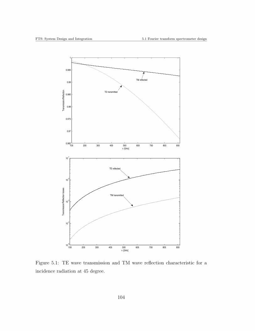
FTS: System Design and Integration 5.1 Fourier transform spectrometer design
100 200 300 400 500 600 700 800 9000.965
0.97
0.975
0.98
0.985
0.99
0.995
1
ν [GHz]
Tran
smiss
ion/
Refle
ctio
n
TE transmitted
TM reflected
100 200 300 400 500 600 700 800 90010
-5
10-4
10-3
10-2
10-1
ν [GHz]
Tran
smiss
ion/
Refle
ctio
n lo
sses
TE reflected
TM transmitted
Figure 5.1: TE wave transmission and TM wave reflection characteristic for a
incidence radiation at 45 degree.
104
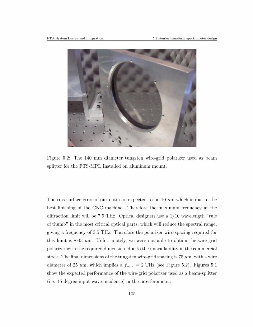
FTS: System Design and Integration 5.1 Fourier transform spectrometer design
Figure 5.2: The 140 mm diameter tungsten wire-grid polarizer used as beam
splitter for the FTS-MPI. Installed on aluminum mount.
The rms surface error of our optics is expected to be 10 µm which is due to the
best finishing of the CNC machine. Therefore the maximum frequency at the
diffraction limit will be 7.5 THz. Optical designers use a 1/10 wavelength ”rule
of thumb” in the most critical optical parts, which will reduce the spectral range,
giving a frequency of 3.5 THz. Therefore the polarizer wire-spacing required for
this limit is ∼43 µm. Unfortunately, we were not able to obtain the wire-grid
polarizer with the required dimension, due to the unavailability in the commercial
stock. The final dimensions of the tungsten wire-grid spacing is 75 µm, with a wire
diameter of 25 µm, which implies a fmax = 2 THz (see Figure 5.2). Figures 5.1
show the expected performance of the wire-grid polarizer used as a beam-splitter
(i.e. 45 degree input wave incidence) in the interferometer.
105
FTS: System Design and Integration 5.1 Fourier transform spectrometer design
5.1.3 System throughput of the system
Initially the coupling optics of the system used a feed-horn with a focal ratio of 2.4
and an acceptance angle of 12 degrees. For this large acceptance angle, we had to
use a copper table to raise the feed-horn and place it closer to the vacuum window
in order to avoid vignetting. As was explained in section 4.2.3, this configuration
is prone to temperature instability. The effective focal length of the system must
be short in order to avoid a large-diameter optics that feed the concentrating
horn with a 12 degrees acceptance angle. The use of large-optics is not really
inconvenient, but it increases the cost of the system, due mainly to the polarizers
which are the most expensive items. Consequently the size of the interferometer
optics will be driven by the design of a good thermal stabilization of the detection
system, and for a suitable frequency range that constrains the useful dimensions
of the feed optics. Thus, in order to have a thermally-stable system, the coupling
optics should be placed in direct contact to with the cryostat base-plate. The
large acceptance angle of the original feed-horn however will cause the vacuum
window to vignette the beam. Therefore we decided to change the coupling optics
in order to have a clean beam through the vacuum window.
We establish the diameter of the focusing optics to be a value of 127 mm and
the focal distance to be 610 mm. Therefore the f -number of the focusing optics is
4.8. With these parameters we are able to obtain the Winston-Cone dimensions.
The acceptance angle of the Winston-cone feed-horn is
θ1 = arcsin
(
1
2ffo
)
, (5.2)
where ffo is the focal ratio of the focusing optics. Then fixing the angular diam-
eter of the field of view to 1 degree, we can calculate the diameters of the input
and output apertures, and the feed-horn length, using Eqs. 4.9, 4.10 and 4.11.
The physical dimensions are shown in table 5.1.
The focusing mirror is a 90 degree off-axis parabolic mirror with an effective
106
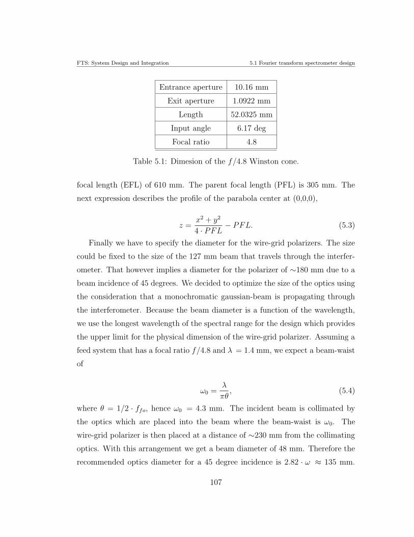
FTS: System Design and Integration 5.1 Fourier transform spectrometer design
Entrance aperture 10.16 mm
Exit aperture 1.0922 mm
Length 52.0325 mm
Input angle 6.17 deg
Focal ratio 4.8
Table 5.1: Dimesion of the f/4.8 Winston cone.
focal length (EFL) of 610 mm. The parent focal length (PFL) is 305 mm. The
next expression describes the profile of the parabola center at (0,0,0),
z =x2 + y2
4 · PFL− PFL. (5.3)
Finally we have to specify the diameter for the wire-grid polarizers. The size
could be fixed to the size of the 127 mm beam that travels through the interfer-
ometer. That however implies a diameter for the polarizer of ∼180 mm due to a
beam incidence of 45 degrees. We decided to optimize the size of the optics using
the consideration that a monochromatic gaussian-beam is propagating through
the interferometer. Because the beam diameter is a function of the wavelength,
we use the longest wavelength of the spectral range for the design which provides
the upper limit for the physical dimension of the wire-grid polarizer. Assuming a
feed system that has a focal ratio f/4.8 and λ = 1.4 mm, we expect a beam-waist
of
ω0 =λ
πθ, (5.4)
where θ = 1/2 · ffo, hence ω0 = 4.3 mm. The incident beam is collimated by
the optics which are placed into the beam where the beam-waist is ω0. The
wire-grid polarizer is then placed at a distance of ∼230 mm from the collimating
optics. With this arrangement we get a beam diameter of 48 mm. Therefore the
recommended optics diameter for a 45 degree incidence is 2.82 · ω ≈ 135 mm.
107
FTS: System Design and Integration 5.2 Optics machining
The available size for the wire-grid polarizer was 140 mm, which was sufficiently
close to the required size.
5.2 Optics machining
All the reflecting optics of the interferometer were fabricated at the Aspheric
Laboratory of INAOE. The roof mirrors were fabricated into two sections in order
to have a better definition of the roof-line. After machining they were polished
at the optics shop to improve the flatness, the reflection, and consequently, the
optical surface quality.
The interferometer has two identical off-axis parabolic mirrors for collimating
and focusing. Both mirrors were fabricated with a CNC machine. The surface
generation was provided by spline fitting of the CNC to the data points, which we
provided. This method gave as result the best optical quality. Figure 5.3 shows
the first step of the machining process, and figure 5.4 shows the final surface
quality achieved by the CNC. We avoided polishing these mirrors because we
were not able to test the surface quality during the process.
108
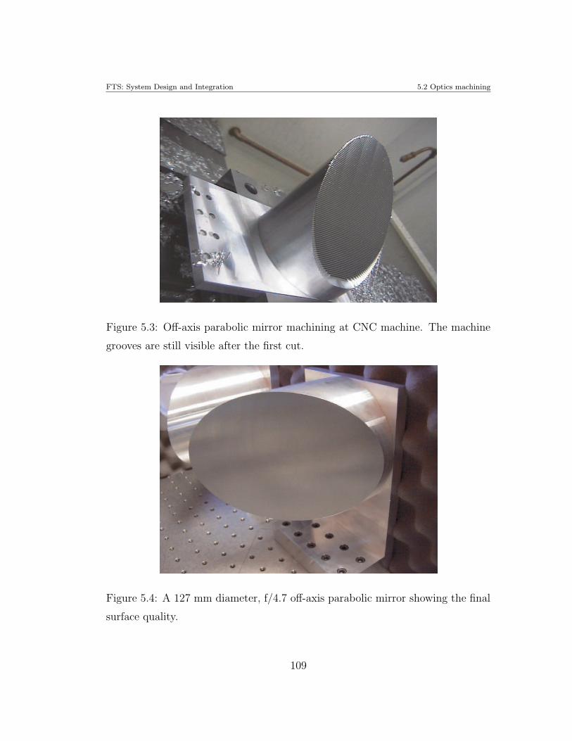
FTS: System Design and Integration 5.2 Optics machining
Figure 5.3: Off-axis parabolic mirror machining at CNC machine. The machine
grooves are still visible after the first cut.
Figure 5.4: A 127 mm diameter, f/4.7 off-axis parabolic mirror showing the final
surface quality.
109
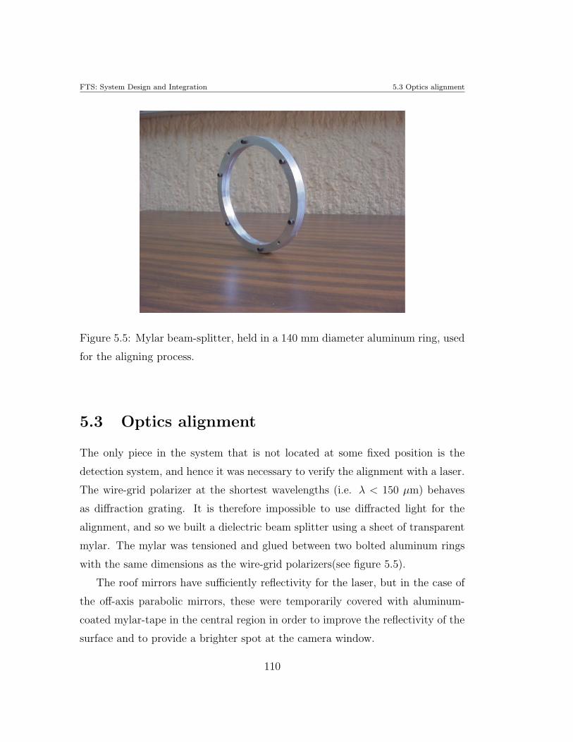
FTS: System Design and Integration 5.3 Optics alignment
Figure 5.5: Mylar beam-splitter, held in a 140 mm diameter aluminum ring, used
for the aligning process.
5.3 Optics alignment
The only piece in the system that is not located at some fixed position is the
detection system, and hence it was necessary to verify the alignment with a laser.
The wire-grid polarizer at the shortest wavelengths (i.e. λ < 150 µm) behaves
as diffraction grating. It is therefore impossible to use diffracted light for the
alignment, and so we built a dielectric beam splitter using a sheet of transparent
mylar. The mylar was tensioned and glued between two bolted aluminum rings
with the same dimensions as the wire-grid polarizers(see figure 5.5).
The roof mirrors have sufficiently reflectivity for the laser, but in the case of
the off-axis parabolic mirrors, these were temporarily covered with aluminum-
coated mylar-tape in the central region in order to improve the reflectivity of the
surface and to provide a brighter spot at the camera window.
110
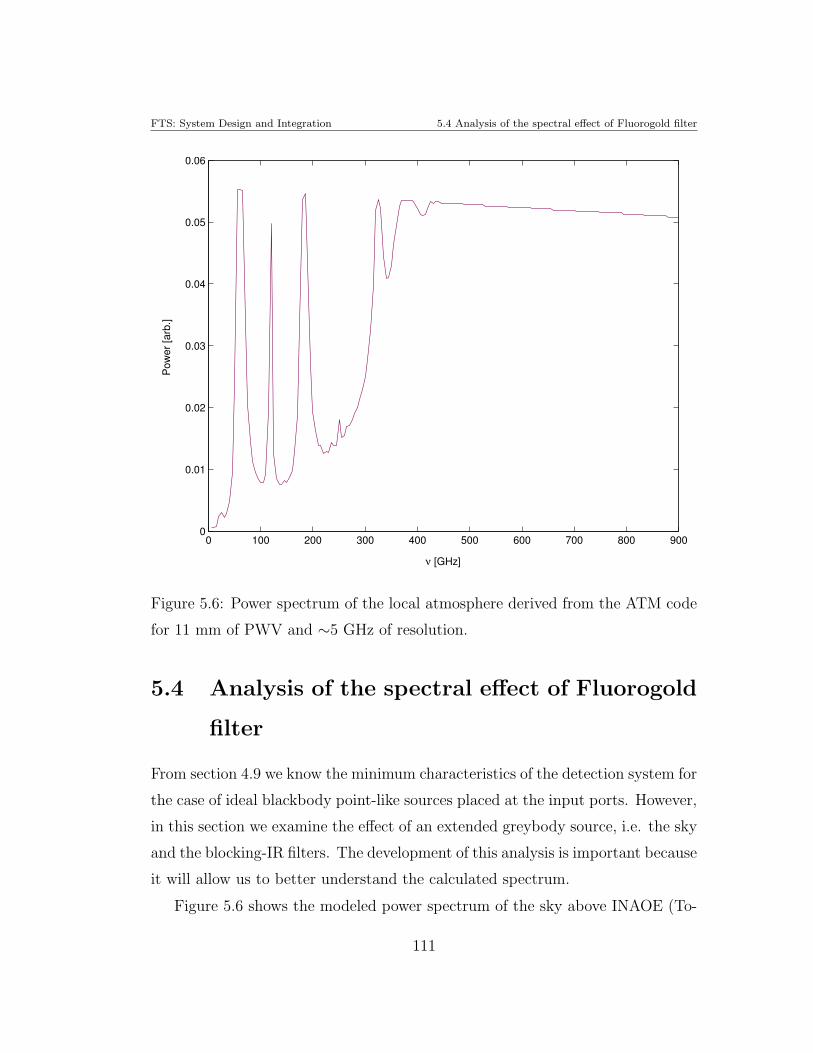
FTS: System Design and Integration 5.4 Analysis of the spectral effect of Fluorogold filter
0 100 200 300 400 500 600 700 800 9000
0.01
0.02
0.03
0.04
0.05
0.06
ν [GHz]
Pow
er [a
rb.]
Figure 5.6: Power spectrum of the local atmosphere derived from the ATM code
for 11 mm of PWV and ∼5 GHz of resolution.
5.4 Analysis of the spectral effect of Fluorogold
filter
From section 4.9 we know the minimum characteristics of the detection system for
the case of ideal blackbody point-like sources placed at the input ports. However,
in this section we examine the effect of an extended greybody source, i.e. the sky
and the blocking-IR filters. The development of this analysis is important because
it will allow us to better understand the calculated spectrum.
Figure 5.6 shows the modeled power spectrum of the sky above INAOE (To-
111
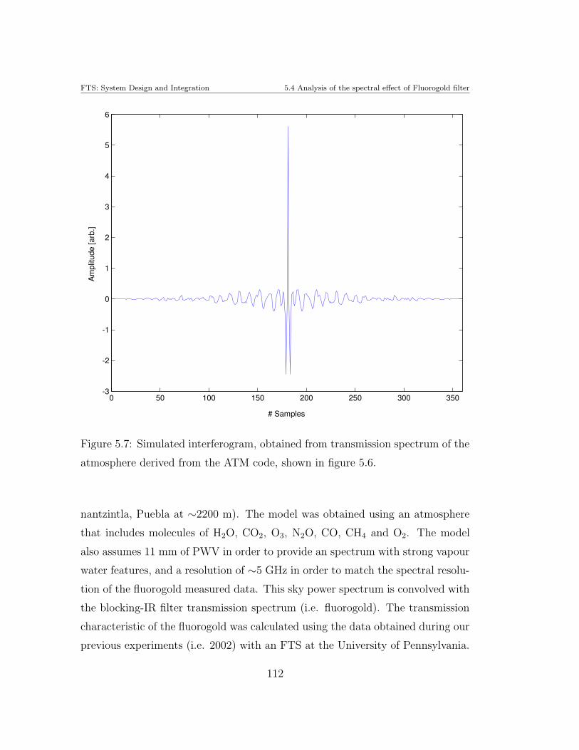
FTS: System Design and Integration 5.4 Analysis of the spectral effect of Fluorogold filter
0 50 100 150 200 250 300 350-3
-2
-1
0
1
2
3
4
5
6
# Samples
Am
plitu
de [a
rb.]
Figure 5.7: Simulated interferogram, obtained from transmission spectrum of the
atmosphere derived from the ATM code, shown in figure 5.6.
nantzintla, Puebla at ∼2200 m). The model was obtained using an atmosphere
that includes molecules of H2O, CO2, O3, N2O, CO, CH4 and O2. The model
also assumes 11 mm of PWV in order to provide an spectrum with strong vapour
water features, and a resolution of ∼5 GHz in order to match the spectral resolu-
tion of the fluorogold measured data. This sky power spectrum is convolved with
the blocking-IR filter transmission spectrum (i.e. fluorogold). The transmission
characteristic of the fluorogold was calculated using the data obtained during our
previous experiments (i.e. 2002) with an FTS at the University of Pennsylvania.
112
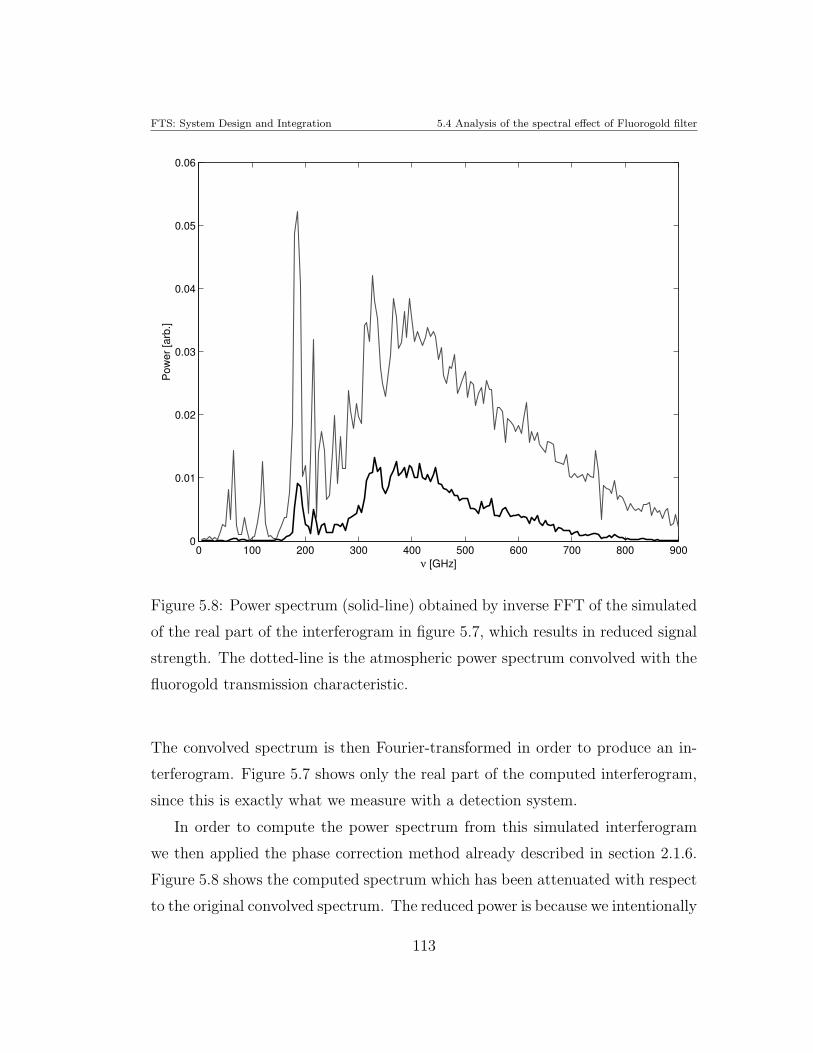
FTS: System Design and Integration 5.4 Analysis of the spectral effect of Fluorogold filter
0 100 200 300 400 500 600 700 800 9000
0.01
0.02
0.03
0.04
0.05
0.06
ν [GHz]
Pow
er [a
rb.]
Figure 5.8: Power spectrum (solid-line) obtained by inverse FFT of the simulated
of the real part of the interferogram in figure 5.7, which results in reduced signal
strength. The dotted-line is the atmospheric power spectrum convolved with the
fluorogold transmission characteristic.
The convolved spectrum is then Fourier-transformed in order to produce an in-
terferogram. Figure 5.7 shows only the real part of the computed interferogram,
since this is exactly what we measure with a detection system.
In order to compute the power spectrum from this simulated interferogram
we then applied the phase correction method already described in section 2.1.6.
Figure 5.8 shows the computed spectrum which has been attenuated with respect
to the original convolved spectrum. The reduced power is because we intentionally
113
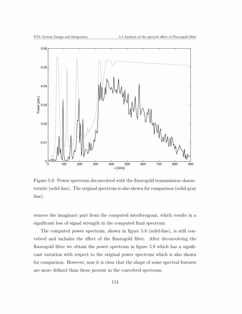
FTS: System Design and Integration 5.4 Analysis of the spectral effect of Fluorogold filter
0 100 200 300 400 500 600 700 800 9000
0.01
0.02
0.03
0.04
0.05
0.06
ν [GHz]
Pow
er [a
rb.]
Figure 5.9: Power spectrum deconvolved with the fluorogold transmission charac-
teristic (solid line). The original spectrum is also shown for comparison (solid-gray
line).
remove the imaginary part from the computed interferogram, which results in a
significant loss of signal strength in the computed final spectrum.
The computed power spectrum, shown in figure 5.8 (solid-line), is still con-
volved and includes the effect of the fluorogold filter. After deconvolving the
fluorogold filter we obtain the power spectrum in figure 5.9 which has a signifi-
cant variation with respect to the original power spectrum which is also shown
for comparison. However, now it is clear that the shape of some spectral features
are more defined than those present in the convolved spectrum.
114
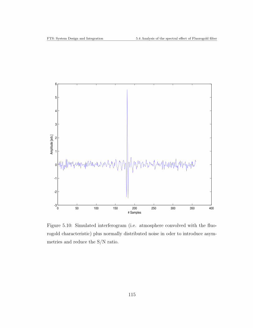
FTS: System Design and Integration 5.4 Analysis of the spectral effect of Fluorogold filter
0 50 100 150 200 250 300 350 400-3
-2
-1
0
1
2
3
4
5
6
# Samples
Ampl
itude
[arb
.]
Figure 5.10: Simulated interferogram (i.e. atmosphere convolved with the fluo-
rogold characteristic) plus normally distributed noise in oder to introduce asym-
metries and reduce the S/N ratio.
115
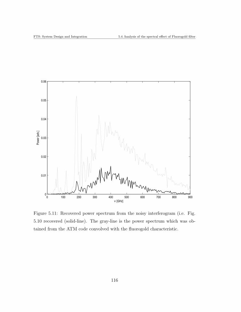
FTS: System Design and Integration 5.4 Analysis of the spectral effect of Fluorogold filter
0 100 200 300 400 500 600 700 800 9000
0.01
0.02
0.03
0.04
0.05
0.06
ν [GHz]
Powe
r [ar
b.]
Figure 5.11: Recovered power spectrum from the noisy interferogram (i.e. Fig.
5.10 recovered (solid-line). The gray-line is the power spectrum which was ob-
tained from the ATM code convolved with the fluorogold characteristic.
116
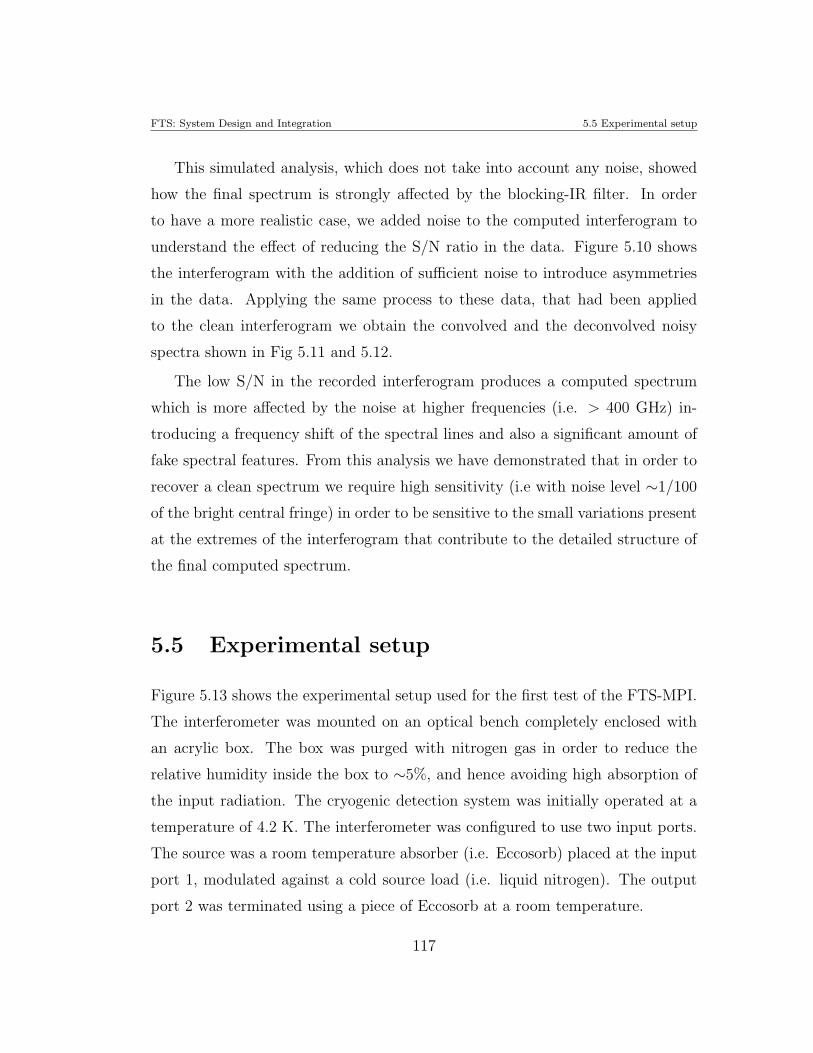
FTS: System Design and Integration 5.5 Experimental setup
This simulated analysis, which does not take into account any noise, showed
how the final spectrum is strongly affected by the blocking-IR filter. In order
to have a more realistic case, we added noise to the computed interferogram to
understand the effect of reducing the S/N ratio in the data. Figure 5.10 shows
the interferogram with the addition of sufficient noise to introduce asymmetries
in the data. Applying the same process to these data, that had been applied
to the clean interferogram we obtain the convolved and the deconvolved noisy
spectra shown in Fig 5.11 and 5.12.
The low S/N in the recorded interferogram produces a computed spectrum
which is more affected by the noise at higher frequencies (i.e. > 400 GHz) in-
troducing a frequency shift of the spectral lines and also a significant amount of
fake spectral features. From this analysis we have demonstrated that in order to
recover a clean spectrum we require high sensitivity (i.e with noise level ∼1/100
of the bright central fringe) in order to be sensitive to the small variations present
at the extremes of the interferogram that contribute to the detailed structure of
the final computed spectrum.
5.5 Experimental setup
Figure 5.13 shows the experimental setup used for the first test of the FTS-MPI.
The interferometer was mounted on an optical bench completely enclosed with
an acrylic box. The box was purged with nitrogen gas in order to reduce the
relative humidity inside the box to ∼5%, and hence avoiding high absorption of
the input radiation. The cryogenic detection system was initially operated at a
temperature of 4.2 K. The interferometer was configured to use two input ports.
The source was a room temperature absorber (i.e. Eccosorb) placed at the input
port 1, modulated against a cold source load (i.e. liquid nitrogen). The output
port 2 was terminated using a piece of Eccosorb at a room temperature.
117
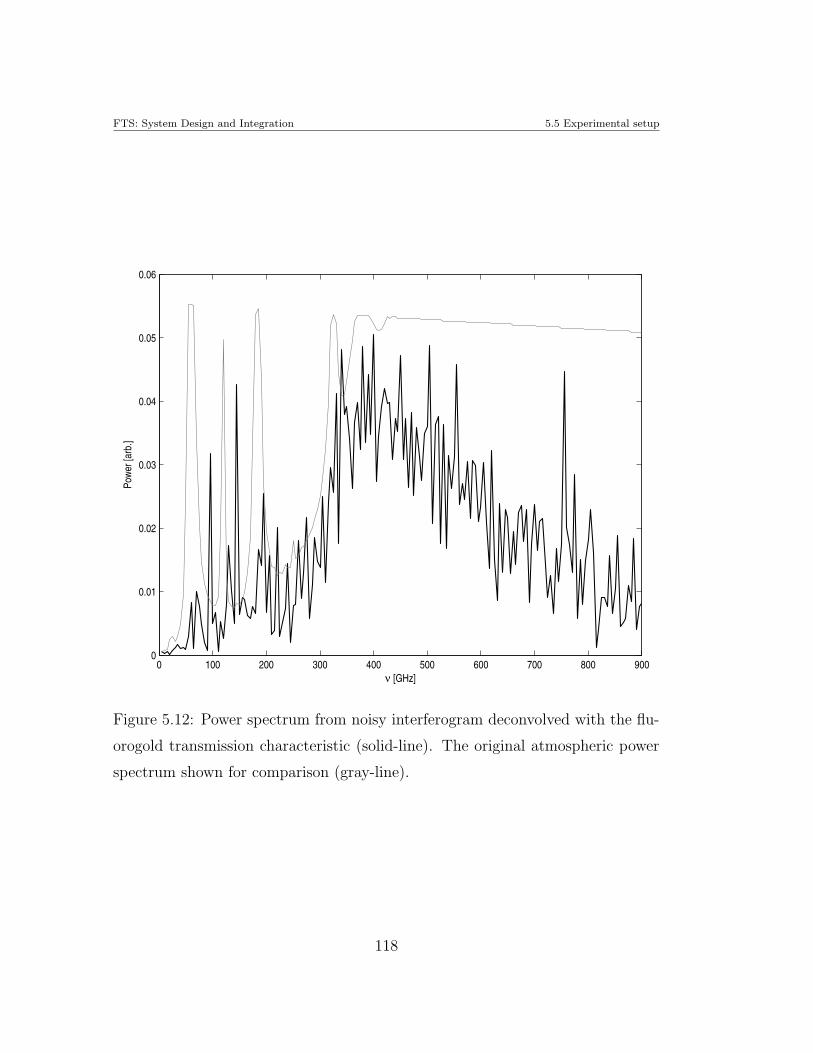
FTS: System Design and Integration 5.5 Experimental setup
0 100 200 300 400 500 600 700 800 9000
0.01
0.02
0.03
0.04
0.05
0.06
ν [GHz]
Powe
r [ar
b.]
Figure 5.12: Power spectrum from noisy interferogram deconvolved with the flu-
orogold transmission characteristic (solid-line). The original atmospheric power
spectrum shown for comparison (gray-line).
118
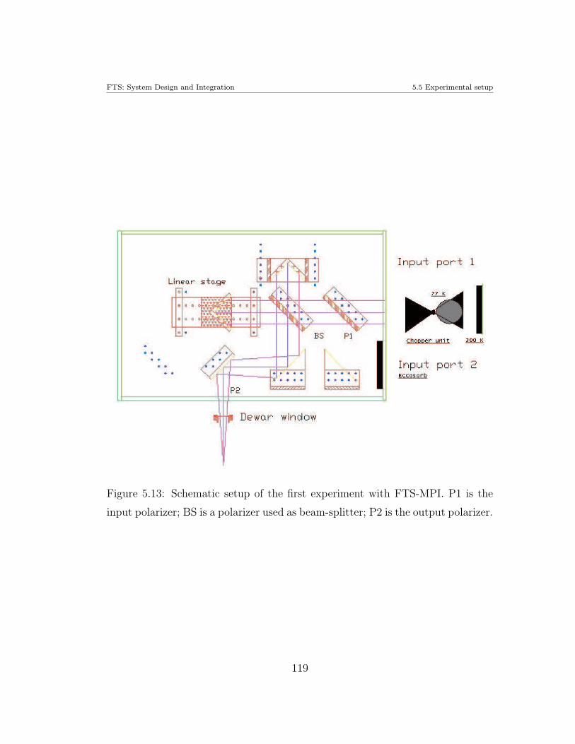
FTS: System Design and Integration 5.5 Experimental setup
Figure 5.13: Schematic setup of the first experiment with FTS-MPI. P1 is the
input polarizer; BS is a polarizer used as beam-splitter; P2 is the output polarizer.
119
FTS: System Design and Integration 5.5 Experimental setup
5.5.1 Chopper Stability
Before describing the results obtained during the initial tests with this setup, it
is necessary to present some effects of the frequency stability for the chopper. In
0 500 1000 1500 2000 2500 3000 3500 4000-4
-3.5
-3
-2.5
-2
-1.5
-1
-0.5
Time(seconds)
Vol
ts
0 1 2 3 4 5 6 7 8 9 1010
-8
10-6
10-4
10-2
100
Frequency (Hz)
PS
D (V
/Hz1 /2
)
Figure 5.14: Top panel: Interferogram record which shows large spikes due to
an unlocked signal events. These events are related to a bad reference signal
generation. Bottom panel shows the PDS of the interferogram record.
order to have a better sensitivity and noise-rejection of the incoming signal, we
use a phase-sensitive device (PSD) amplifier. This device demodulates the signal
that only matches the reference frequency. Hence any other signal, at different
frequencies will not be amplified.
120
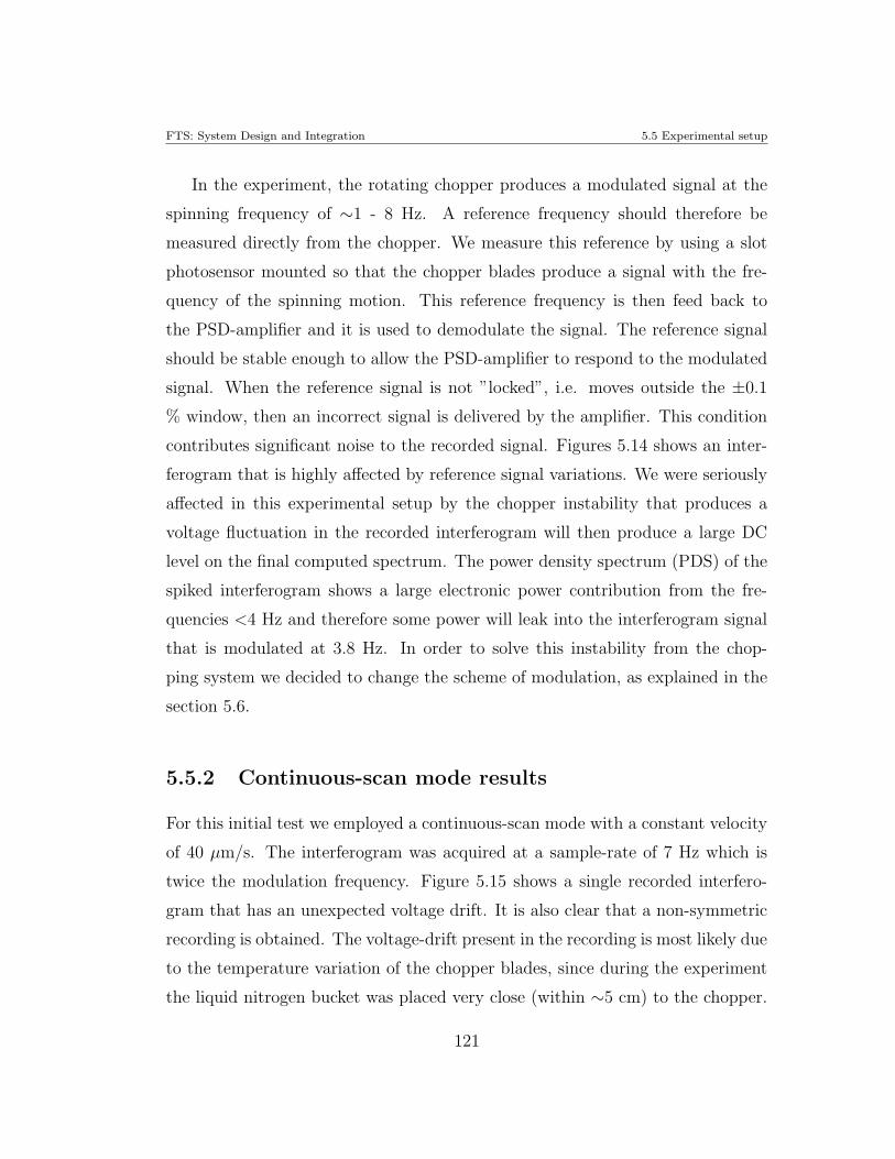
FTS: System Design and Integration 5.5 Experimental setup
In the experiment, the rotating chopper produces a modulated signal at the
spinning frequency of ∼1 - 8 Hz. A reference frequency should therefore be
measured directly from the chopper. We measure this reference by using a slot
photosensor mounted so that the chopper blades produce a signal with the fre-
quency of the spinning motion. This reference frequency is then feed back to
the PSD-amplifier and it is used to demodulate the signal. The reference signal
should be stable enough to allow the PSD-amplifier to respond to the modulated
signal. When the reference signal is not ”locked”, i.e. moves outside the ±0.1
% window, then an incorrect signal is delivered by the amplifier. This condition
contributes significant noise to the recorded signal. Figures 5.14 shows an inter-
ferogram that is highly affected by reference signal variations. We were seriously
affected in this experimental setup by the chopper instability that produces a
voltage fluctuation in the recorded interferogram will then produce a large DC
level on the final computed spectrum. The power density spectrum (PDS) of the
spiked interferogram shows a large electronic power contribution from the fre-
quencies <4 Hz and therefore some power will leak into the interferogram signal
that is modulated at 3.8 Hz. In order to solve this instability from the chop-
ping system we decided to change the scheme of modulation, as explained in the
section 5.6.
5.5.2 Continuous-scan mode results
For this initial test we employed a continuous-scan mode with a constant velocity
of 40 µm/s. The interferogram was acquired at a sample-rate of 7 Hz which is
twice the modulation frequency. Figure 5.15 shows a single recorded interfero-
gram that has an unexpected voltage drift. It is also clear that a non-symmetric
recording is obtained. The voltage-drift present in the recording is most likely due
to the temperature variation of the chopper blades, since during the experiment
the liquid nitrogen bucket was placed very close (within ∼5 cm) to the chopper.
121
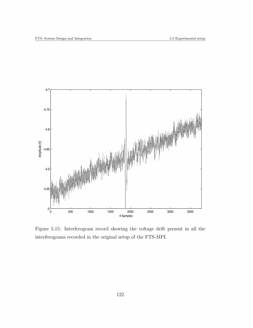
FTS: System Design and Integration 5.5 Experimental setup
0 500 1000 1500 2000 2500 3000 3500-5
-4.95
-4.9
-4.85
-4.8
-4.75
-4.7
# Samples
Ampl
itude
[V]
Figure 5.15: Interferogram record showing the voltage drift present in all the
interferograms recorded in the original setup of the FTS-MPI.
122
FTS: System Design and Integration 5.5 Experimental setup
This reduced the temperature of the chopper blades and hence a change in the
power emitted towards the interferometer.
We also observe a low S/N ratio at the position of the secondary lobes of
the interferogram, which will have a negative impact on the final computed spec-
trum, as explained in section 5.4. In order to improve this situation we co-added
multiple interferograms which improve the S/N ratio of the secondary lobes. Fig-
ure 5.16 shows the details around of the central bright fringe of a combined set of
4 interferograms (top-right panel) that demonstrate a great amount of constant
features which, by means of co-addition, can improve the interferogram.
In order to compute the spectrum we first remove the voltage drift and the
voltage DC level of each interferogram which has the effect of eliminating the
unwanted large DC component in the final computed spectrum. We performed
the voltage-drift correction by taking equally-spaced points (i.e. 20 samples)
along the entire interferogram, to which we applied a linear fit. This simultane-
ously removes the voltage drift as well as the DC level. The bottom-left panel in
Figure 5.16 shows a fully processed interferogram (averaged from 4 records and
DC corrected) which improves the S/N ratio around the central bright fringe, al-
though there is still noise at both ends of the interferograms as well as significants
drifts in the signal on scales of 200 - 300 samples (i.e. ∼1 to 1.5 mm of movement
along the track). This does not implies that the screw-thread is not constant
because, the effect is not present in the step-integrate scan mode. Figure 5.17
shows a set of averaged interferograms obtained during the continuous-scan mode
tests. The first, the second and third row are records looking at the sky and the
fourth row shows a record looking at a room temperature absorber. Each one
is the average of 5 interferograms recorded in period of 5 minutes. Each aver-
aged interferogram is then Fourier-transformed in order to compute its spectrum.
Figure 5.17 also shows the respective spectrum without phase correction and fre-
quency calibration. From the graphs we see a constant shape that is the result of
the instrument profile plus the transmission profile introduced by the flourogold
123
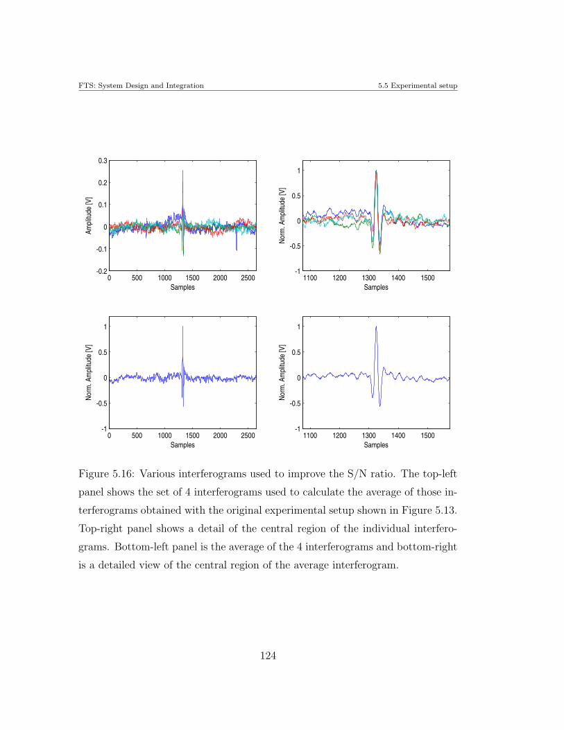
FTS: System Design and Integration 5.5 Experimental setup
0 500 1000 1500 2000 2500-0.2
-0.1
0
0.1
0.2
0.3
Samples
Ampl
itude
[V]
1100 1200 1300 1400 1500-1
-0.5
0
0.5
1
SamplesNo
rm. A
mpl
itude
[V]
0 500 1000 1500 2000 2500-1
-0.5
0
0.5
1
Samples
Norm
. Am
plitu
de [V
]
1100 1200 1300 1400 1500-1
-0.5
0
0.5
1
Samples
Norm
. Am
plitu
de [V
]
Figure 5.16: Various interferograms used to improve the S/N ratio. The top-left
panel shows the set of 4 interferograms used to calculate the average of those in-
terferograms obtained with the original experimental setup shown in Figure 5.13.
Top-right panel shows a detail of the central region of the individual interfero-
grams. Bottom-left panel is the average of the 4 interferograms and bottom-right
is a detailed view of the central region of the average interferogram.
124
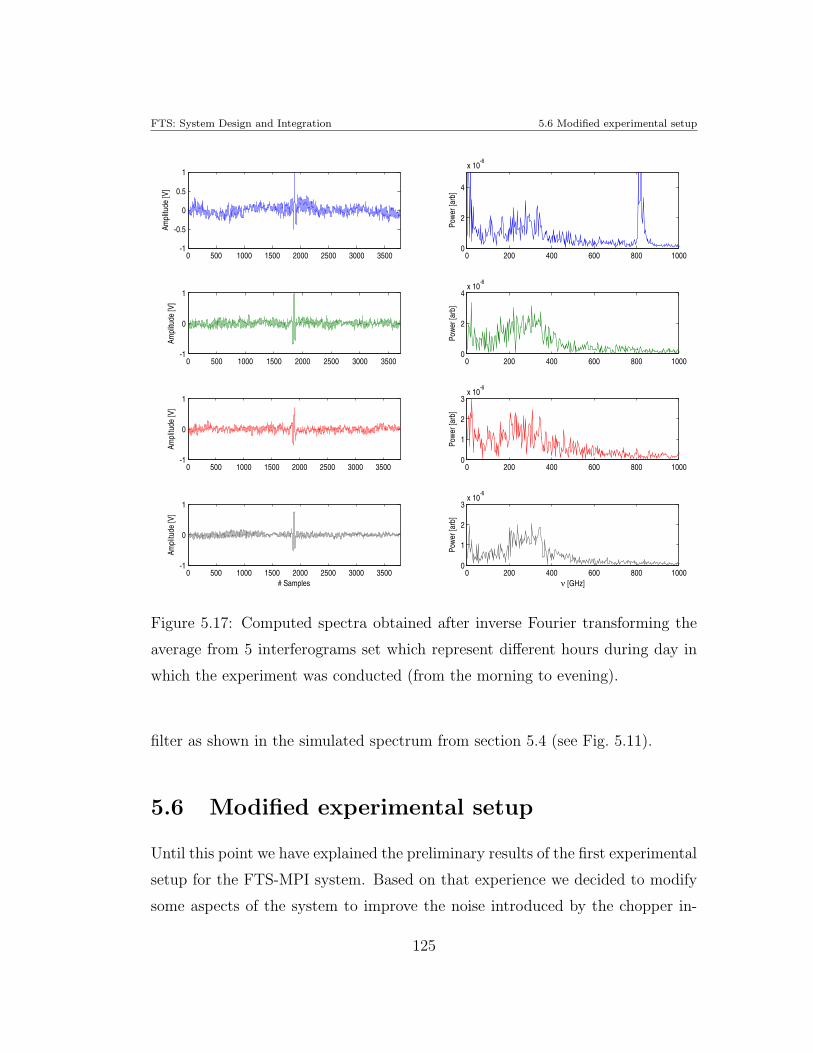
FTS: System Design and Integration 5.6 Modified experimental setup
0 500 1000 1500 2000 2500 3000 3500-1
-0.5
0
0.5
1Am
plitu
de [V
]
0 500 1000 1500 2000 2500 3000 3500-1
0
1
Ampl
itude
[V]
0 500 1000 1500 2000 2500 3000 3500-1
0
1
Ampl
itude
[V]
0 500 1000 1500 2000 2500 3000 3500-1
0
1
# Samples
Ampl
itude
[V]
0 200 400 600 800 10000
2
4
x 10-6
Powe
r [ar
b]
0 200 400 600 800 10000
2
4x 10
-6
Powe
r [ar
b]
0 200 400 600 800 10000
1
2
3x 10
-6
Powe
r [ar
b]
0 200 400 600 800 10000
1
2
3x 10
-6
ν [GHz]
Powe
r [ar
b]
Figure 5.17: Computed spectra obtained after inverse Fourier transforming the
average from 5 interferograms set which represent different hours during day in
which the experiment was conducted (from the morning to evening).
filter as shown in the simulated spectrum from section 5.4 (see Fig. 5.11).
5.6 Modified experimental setup
Until this point we have explained the preliminary results of the first experimental
setup for the FTS-MPI system. Based on that experience we decided to modify
some aspects of the system to improve the noise introduced by the chopper in-
125
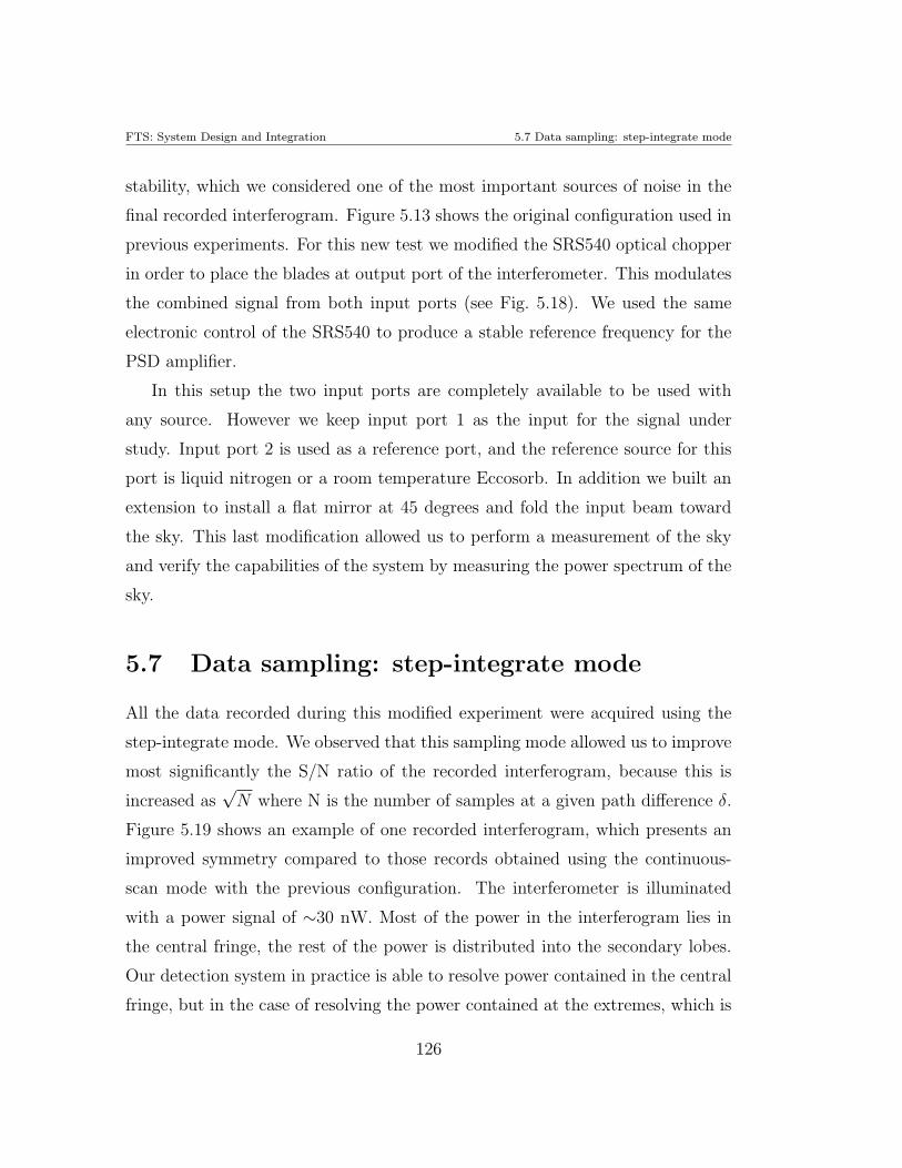
FTS: System Design and Integration 5.7 Data sampling: step-integrate mode
stability, which we considered one of the most important sources of noise in the
final recorded interferogram. Figure 5.13 shows the original configuration used in
previous experiments. For this new test we modified the SRS540 optical chopper
in order to place the blades at output port of the interferometer. This modulates
the combined signal from both input ports (see Fig. 5.18). We used the same
electronic control of the SRS540 to produce a stable reference frequency for the
PSD amplifier.
In this setup the two input ports are completely available to be used with
any source. However we keep input port 1 as the input for the signal under
study. Input port 2 is used as a reference port, and the reference source for this
port is liquid nitrogen or a room temperature Eccosorb. In addition we built an
extension to install a flat mirror at 45 degrees and fold the input beam toward
the sky. This last modification allowed us to perform a measurement of the sky
and verify the capabilities of the system by measuring the power spectrum of the
sky.
5.7 Data sampling: step-integrate mode
All the data recorded during this modified experiment were acquired using the
step-integrate mode. We observed that this sampling mode allowed us to improve
most significantly the S/N ratio of the recorded interferogram, because this is
increased as√
N where N is the number of samples at a given path difference δ.
Figure 5.19 shows an example of one recorded interferogram, which presents an
improved symmetry compared to those records obtained using the continuous-
scan mode with the previous configuration. The interferometer is illuminated
with a power signal of ∼30 nW. Most of the power in the interferogram lies in
the central fringe, the rest of the power is distributed into the secondary lobes.
Our detection system in practice is able to resolve power contained in the central
fringe, but in the case of resolving the power contained at the extremes, which is
126
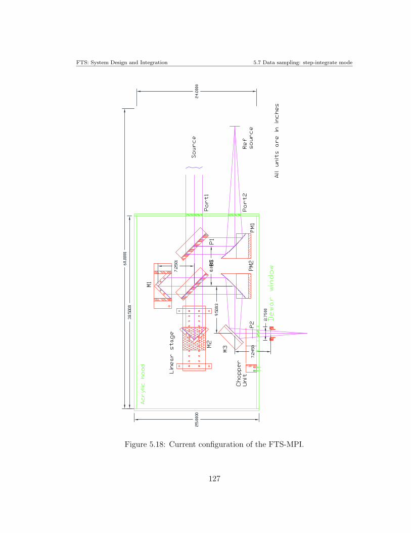
FTS: System Design and Integration 5.7 Data sampling: step-integrate mode
Figure 5.18: Current configuration of the FTS-MPI.
127
FTS: System Design and Integration 5.7 Data sampling: step-integrate mode
0 0.25 0.5 0.75 1 1.25 1.5-1.5
-1
-0.5
0
0.5
1
Relative position [cm]
Ampl
itude
[vol
ts]
Figure 5.19: Interferogram recorded using step-integrate mode, looking the sky.
about to 3×10⁴ smaller than the central fringe, we expect to be at the limit of the
detection system. The expected power contained at the extremes is ∼1 pW. The
NEP, in terms of a required S/N∼4, should then be ∼ 1 × 10⁻¹³ W/Hz1/2. The
measured NEP of our detection system at 3.9 K is ∼ 1.5×10⁻¹⁴ W/Hz1/2 which in
practice should provide ∼70 times the required S/N. Figure 5.20 shows the signal
to noise ratio of each sample as a function of its position in a single interferogram
record. The faintest ends show that the S/N ratio is below the required value
to resolve completely the interferogram. This implies the existence of a extra
source of noise which has not yet been identified. The mean S/N ratio is ∼ .06
128
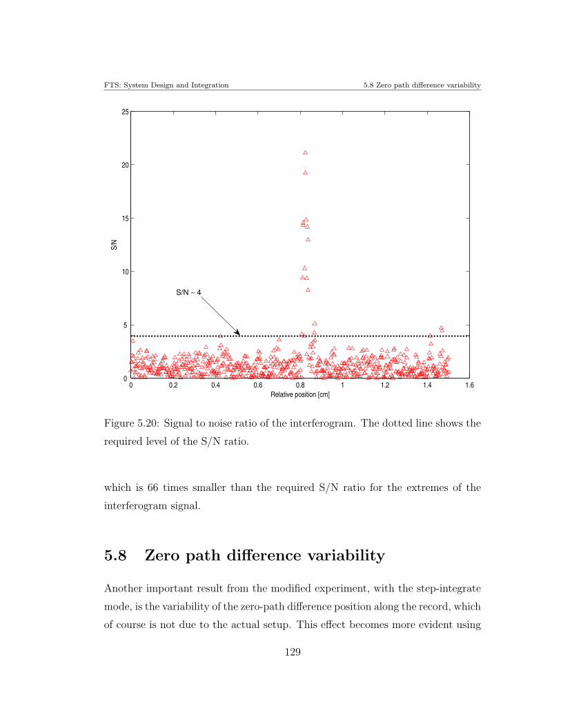
FTS: System Design and Integration 5.8 Zero path difference variability
0 0.2 0.4 0.6 0.8 1 1.2 1.4 1.60
5
10
15
20
25
Relative position [cm]
S/N
S/N ∼ 4
Figure 5.20: Signal to noise ratio of the interferogram. The dotted line shows the
required level of the S/N ratio.
which is 66 times smaller than the required S/N ratio for the extremes of the
interferogram signal.
5.8 Zero path difference variability
Another important result from the modified experiment, with the step-integrate
mode, is the variability of the zero-path difference position along the record, which
of course is not due to the actual setup. This effect becomes more evident using
129
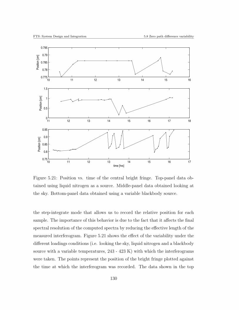
FTS: System Design and Integration 5.8 Zero path difference variability
10 11 12 13 14 15 160.775
0.78
0.785
0.79
0.795
Posit
ion
[cm
]
11 12 13 14 15 16 17 180
0.5
1
1.5
Posit
ion
[cm
]
10 11 12 13 14 15 16 170.75
0.8
0.85
0.9
0.95
time [hrs]
Posit
ion
[cm
]
Figure 5.21: Position vs. time of the central bright fringe. Top-panel data ob-
tained using liquid nitrogen as a source. Middle-panel data obtained looking at
the sky. Bottom-panel data obtained using a variable blackbody source.
the step-integrate mode that allows us to record the relative position for each
sample. The importance of this behavior is due to the fact that it affects the final
spectral resolution of the computed spectra by reducing the effective length of the
measured interferogram. Figure 5.21 shows the effect of the variability under the
different loadings conditions (i.e. looking the sky, liquid nitrogen and a blackbody
source with a variable temperatures, 243 - 423 K) with which the interferograms
were taken. The points represent the position of the bright fringe plotted against
the time at which the interferogram was recorded. The data shown in the top
130
FTS: System Design and Integration 5.9 Computed spectra
panel corresponds to interferograms recorded using a liquid nitrogen as a source,
during a ∼5 h period of time. The same period of time is shown in the middle
panel, in which the source is now the sky. The position of the bright fringe is more
variable than in the previous configuration and 5 times broader. Additionally
large variations were present at the end of the measurements. Finally the bottom
panel shows data taken using a blackbody calibration source with large position
variations during the experiment. We assume that this variability is due mainly
to turbulence in the air close to the input ports. This effect of interferogram-
motion is compared with the observed effect in a laser-illuminated Michelson
interferometer, in which air turbulence in any of the two interferometer arms
or at the input, produces vibrations in the interferogram image. We use liquid
nitrogen as the reference source at input port 2. Because the source is outside
the acrylic box, it will produce local air turbulence due to the convection and
the mixing of hot air and cold nitrogen gas around the container. Also variations
in the power emitted by the source are introduced due to the ice build-up which
changes the transmission properties of the container. This interferogram-motion
effect reduces the effective length of the interferogram and consequently it will
reduce the spectral resolution; furthermore variations in shorter times scales will
produce a noisy interferogram and therefore a low S/N spectrum. The above
should be taken into account in order to improve the performance of the FTS-
MPI. All the modifications to improve the system will have to be done as part of
the future work.
131
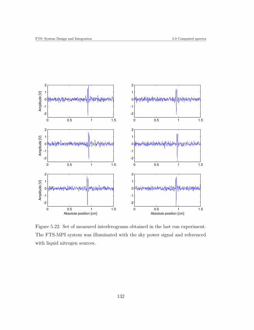
FTS: System Design and Integration 5.9 Computed spectra
0 0.5 1 1.5
-2
-1
0
1
2
Am
plitu
de [V
]
0 0.5 1 1.5
-2
-1
0
1
2
0 0.5 1 1.5
-2
-1
0
1
2
Am
plitu
de [V
]
0 0.5 1 1.5
-2
-1
0
1
2
0 0.5 1 1.5
-2
-1
0
1
2
Absolute position [cm]
Am
plitu
de [V
]
0 0.5 1 1.5
-2
-1
0
1
2
Absolute position [cm]
Figure 5.22: Set of measured interferograms obtained in the last run experiment.
The FTS-MPI system was illuminated with the sky power signal and referenced
with liquid nitrogen sources.
132
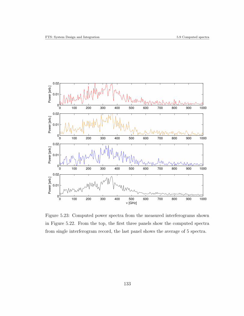
FTS: System Design and Integration 5.9 Computed spectra
0 100 200 300 400 500 600 700 800 900 10000
0.01
0.02
Pow
er [a
rb.]
0 100 200 300 400 500 600 700 800 900 10000
0.01
0.02
Pow
er [a
rb.]
0 100 200 300 400 500 600 700 800 900 10000
0.01
0.02
Pow
er [a
rb.]
0 100 200 300 400 500 600 700 800 900 10000
0.01
0.02
ν [GHz]
Pow
er [a
rb.]
Figure 5.23: Computed power spectra from the measured interferograms shown
in Figure 5.22. From the top, the first three panels show the computed spectra
from single interferogram record, the last panel shows the average of 5 spectra.
133
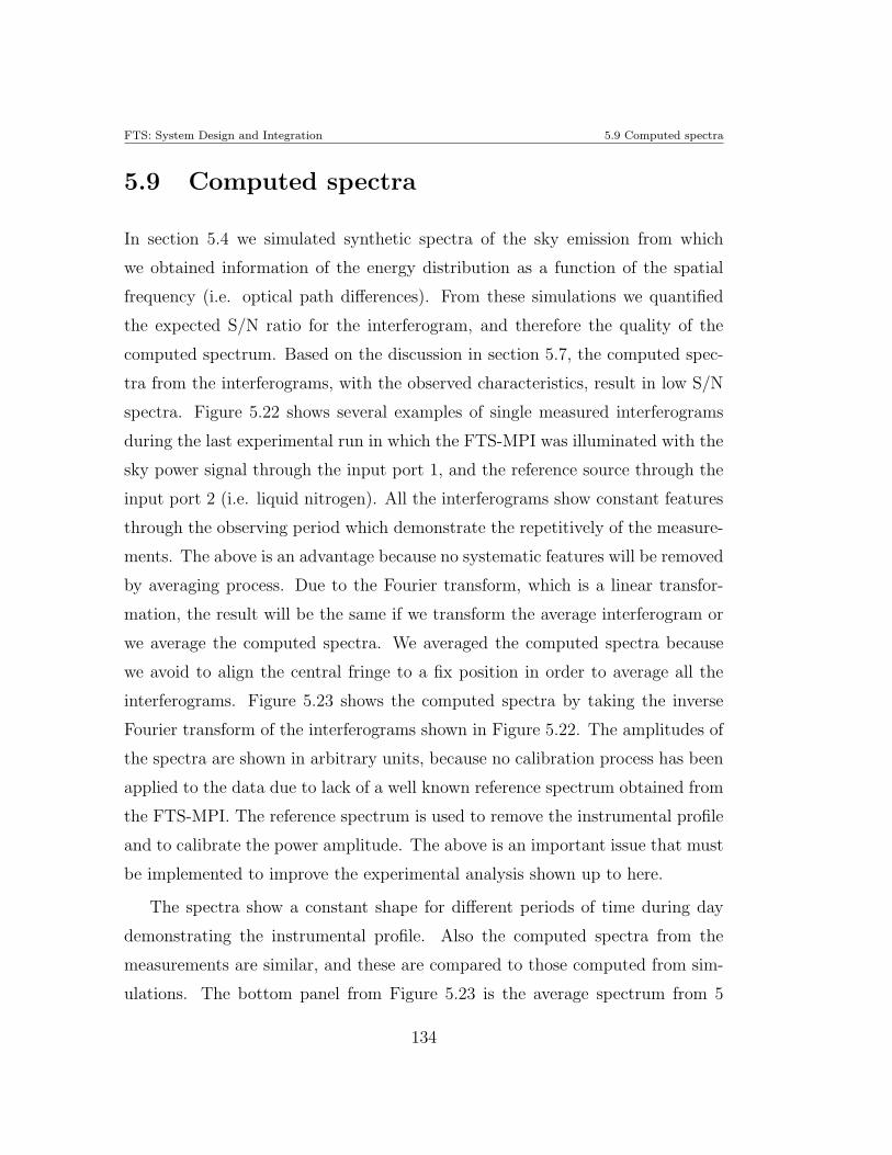
FTS: System Design and Integration 5.9 Computed spectra
5.9 Computed spectra
In section 5.4 we simulated synthetic spectra of the sky emission from which
we obtained information of the energy distribution as a function of the spatial
frequency (i.e. optical path differences). From these simulations we quantified
the expected S/N ratio for the interferogram, and therefore the quality of the
computed spectrum. Based on the discussion in section 5.7, the computed spec-
tra from the interferograms, with the observed characteristics, result in low S/N
spectra. Figure 5.22 shows several examples of single measured interferograms
during the last experimental run in which the FTS-MPI was illuminated with the
sky power signal through the input port 1, and the reference source through the
input port 2 (i.e. liquid nitrogen). All the interferograms show constant features
through the observing period which demonstrate the repetitively of the measure-
ments. The above is an advantage because no systematic features will be removed
by averaging process. Due to the Fourier transform, which is a linear transfor-
mation, the result will be the same if we transform the average interferogram or
we average the computed spectra. We averaged the computed spectra because
we avoid to align the central fringe to a fix position in order to average all the
interferograms. Figure 5.23 shows the computed spectra by taking the inverse
Fourier transform of the interferograms shown in Figure 5.22. The amplitudes of
the spectra are shown in arbitrary units, because no calibration process has been
applied to the data due to lack of a well known reference spectrum obtained from
the FTS-MPI. The reference spectrum is used to remove the instrumental profile
and to calibrate the power amplitude. The above is an important issue that must
be implemented to improve the experimental analysis shown up to here.
The spectra show a constant shape for different periods of time during day
demonstrating the instrumental profile. Also the computed spectra from the
measurements are similar, and these are compared to those computed from sim-
ulations. The bottom panel from Figure 5.23 is the average spectrum from 5
134
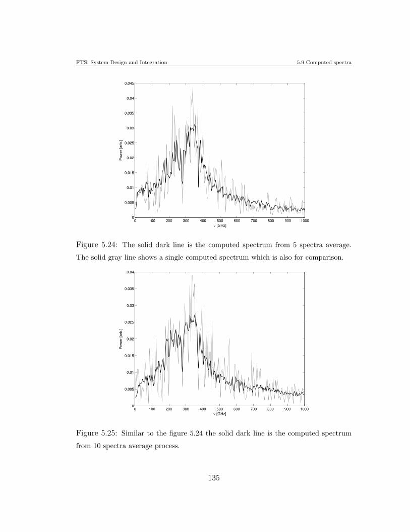
FTS: System Design and Integration 5.9 Computed spectra
0 100 200 300 400 500 600 700 800 900 10000
0.005
0.01
0.015
0.02
0.025
0.03
0.035
0.04
0.045
ν [GHz]
Pow
er [a
rb.]
Figure 5.24: The solid dark line is the computed spectrum from 5 spectra average.
The solid gray line shows a single computed spectrum which is also for comparison.
0 100 200 300 400 500 600 700 800 900 10000
0.005
0.01
0.015
0.02
0.025
0.03
0.035
0.04
ν [GHz]
Pow
er [a
rb.]
Figure 5.25: Similar to the figure 5.24 the solid dark line is the computed spectrum
from 10 spectra average process.
135
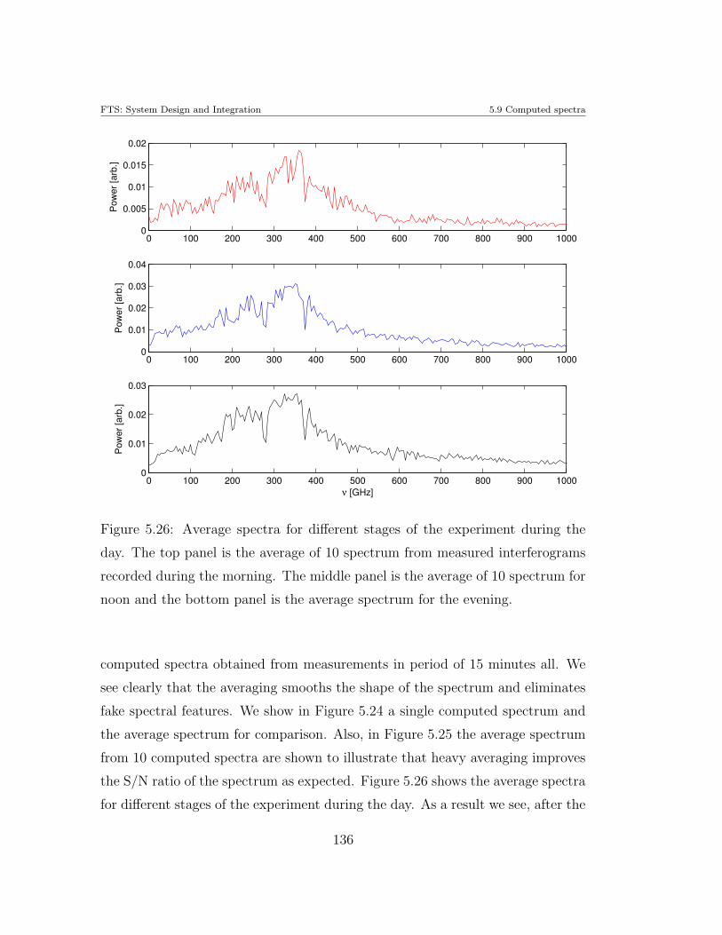
FTS: System Design and Integration 5.9 Computed spectra
0 100 200 300 400 500 600 700 800 900 10000
0.005
0.01
0.015
0.02
Pow
er [a
rb.]
0 100 200 300 400 500 600 700 800 900 10000
0.01
0.02
0.03
0.04
Pow
er [a
rb.]
0 100 200 300 400 500 600 700 800 900 10000
0.01
0.02
0.03
ν [GHz]
Pow
er [a
rb.]
Figure 5.26: Average spectra for different stages of the experiment during the
day. The top panel is the average of 10 spectrum from measured interferograms
recorded during the morning. The middle panel is the average of 10 spectrum for
noon and the bottom panel is the average spectrum for the evening.
computed spectra obtained from measurements in period of 15 minutes all. We
see clearly that the averaging smooths the shape of the spectrum and eliminates
fake spectral features. We show in Figure 5.24 a single computed spectrum and
the average spectrum for comparison. Also, in Figure 5.25 the average spectrum
from 10 computed spectra are shown to illustrate that heavy averaging improves
the S/N ratio of the spectrum as expected. Figure 5.26 shows the average spectra
for different stages of the experiment during the day. As a result we see, after the
136
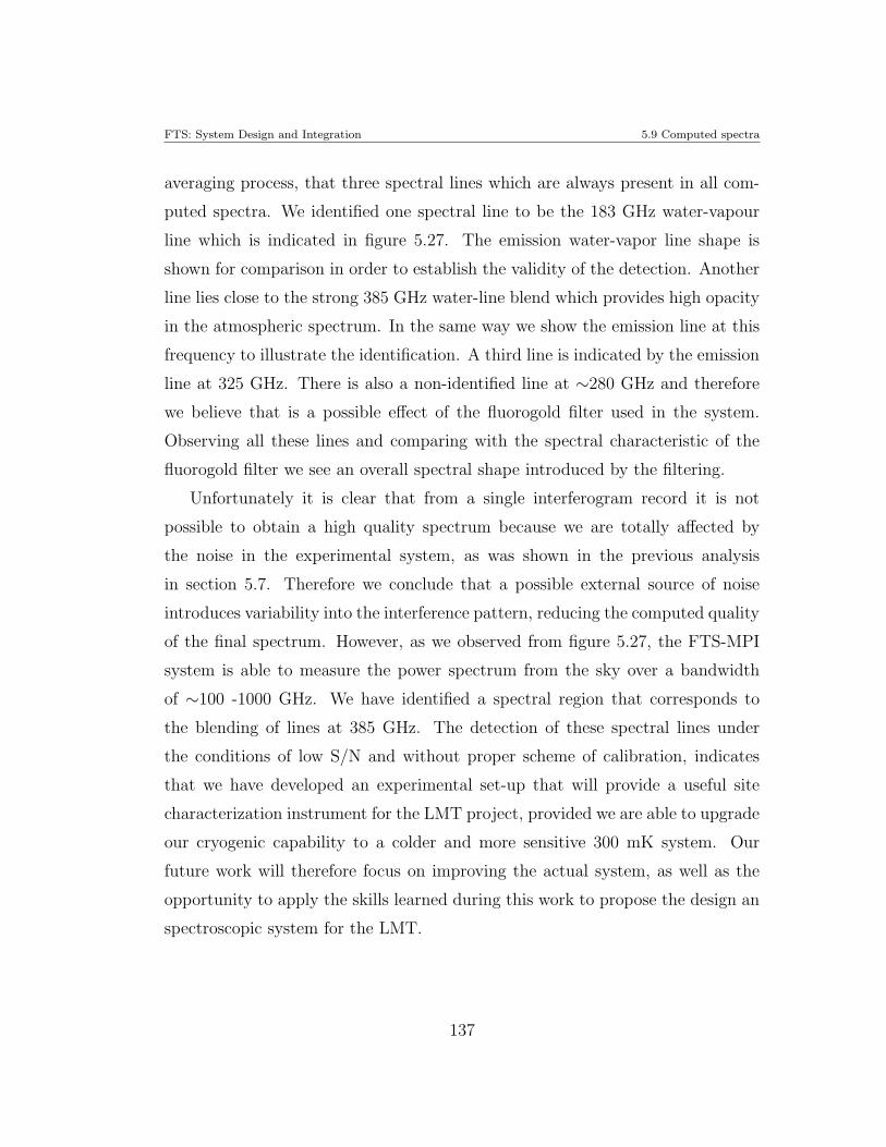
FTS: System Design and Integration 5.9 Computed spectra
averaging process, that three spectral lines which are always present in all com-
puted spectra. We identified one spectral line to be the 183 GHz water-vapour
line which is indicated in figure 5.27. The emission water-vapor line shape is
shown for comparison in order to establish the validity of the detection. Another
line lies close to the strong 385 GHz water-line blend which provides high opacity
in the atmospheric spectrum. In the same way we show the emission line at this
frequency to illustrate the identification. A third line is indicated by the emission
line at 325 GHz. There is also a non-identified line at ∼280 GHz and therefore
we believe that is a possible effect of the fluorogold filter used in the system.
Observing all these lines and comparing with the spectral characteristic of the
fluorogold filter we see an overall spectral shape introduced by the filtering.
Unfortunately it is clear that from a single interferogram record it is not
possible to obtain a high quality spectrum because we are totally affected by
the noise in the experimental system, as was shown in the previous analysis
in section 5.7. Therefore we conclude that a possible external source of noise
introduces variability into the interference pattern, reducing the computed quality
of the final spectrum. However, as we observed from figure 5.27, the FTS-MPI
system is able to measure the power spectrum from the sky over a bandwidth
of ∼100 -1000 GHz. We have identified a spectral region that corresponds to
the blending of lines at 385 GHz. The detection of these spectral lines under
the conditions of low S/N and without proper scheme of calibration, indicates
that we have developed an experimental set-up that will provide a useful site
characterization instrument for the LMT project, provided we are able to upgrade
our cryogenic capability to a colder and more sensitive 300 mK system. Our
future work will therefore focus on improving the actual system, as well as the
opportunity to apply the skills learned during this work to propose the design an
spectroscopic system for the LMT.
137
FTS: System Design and Integration 5.9 Computed spectra
0 100 200 300 400 500 600 700 800 9000
0.1
0.2
0.3
0.4
0.5
0.6
0.7
0.8
0.9
1
ν [GHz]
Nor
mal
ized
pow
er
183 GHz
Blend line at ∼385 GHz
Figure 5.27: Average spectrum from full set of interferograms obtained in the
experimental run observing the sky (solid-dark line). The 183 GHz water-vapour
line and 380, 382, 386 390 and 391 GHz water-vapour blend lines. The vertical-
dotted lines show the position of the central frequency of the measured lines.
138
Chapter 6
Conclusions and Future Work
The goal of the present work was to create the facilities to develop the basic
cryogenic instrumentation for sub-mm/mm wavelengths and to develop basic in-
struments based on bolometric detectors to work in the sub-mm/mm wavelength
regime.
Since this kind of technology has not previously been developed in Mexico,
it was necessary to first learn the experimental skills in this area. Thus first
I started my training with other international groups with great experience in
system design and integration of cryogenic instrumentation. In 2001 I worked for
almost one year at the University of Pennsylvania (UPenn) with the Prof. Mark
Devlin’s group. During this period I was learning the basic skills in cryogenic
systems (∼ 4.2 to 300 mK), vacuum techniques, bolometer characterization, low-
noise read-out electronics as well as optical materials for optical-FIR blocking
filters, and basic skills in mechanical design for cryogenic systems. In 2002 we
spent two months working on a Far-Infrared Fourier Transform Spectrometer
system. I worked on the optical alignment of the FTS and debugging the data
acquisition and control software for the system.
139
Conclusions and Future Work Conclusions and Future Work
The experience obtained during the period 2001-2002, allowed us to begin
establishing the millimetric-instrumentation laboratory at INAOE in 2002. With
the initial MI-Lab facilities I fully characterized a composite bolometer to temper-
atures down to ∼1.5 K. The bolometer is the critical component of our millimetric
camera, used in the FTS-MPI, which was designed as part of the Total Power
Sky-Monitor. The composite bolometer was designed with an NTD:Ge thermistor
from Haller-Beeman Inc. In order to improve the thermal conductance for opera-
tional temperature of ∼1.8 K, we designed a bolometer that used 12 µm diameter,
5 mm length NbTi leads. As result of this characterization we found that the
thermal conductance of the bolometer using these leads at 1.8 K is ∼ 5.5 × 10⁻⁸
W/K, a larger value than the prediction from the design i.e. 3 × 10⁻⁹ W/K.
This resulted in a less sensitive device and a slower time response. However this
experimental result contributes to the knowledge of the thermal properties of the
NbTi leads at temperatures in the range of 1.5 - 3.9 K. I still expected however
that the sensor would be sensitive enough to be used as part of the FTS-MPI
system, since the power-loading conditions are higher than those conditions for
the Total Power Sky-Monitor.
I have presented the development and the design of a Fourier Transform Spec-
trometer of the Martin Puplett type to work at sub-mm/mm wavelengths. In
order to couple the cryogenic camera with the interferometer optics, I modified
the cold optics, which allowed us to eliminate temperature fluctuations present
in early configurations. The coupling was obtained by designing a new aluminum
feed-horn with a f/4.8 focal ratio. The feed-horn and all the interferometer optics
were made at INAOE. This is an important fact to report because it demonstrates
our capabilities to produce complex optics for future sub-mm/mm instruments.
I have shown an analysis of the impact that the IR-blocking filters have on
the instrument response, as well as the techniques used to compute the power
spectrum from the recorded interferogram. An important conclusion from this
analysis is the relation between the S/N ratio and the final computed spectrum.
140
Conclusions and Future Work Conclusions and Future Work
A high S/N ratio in the secondary lobes will naturally produce a computed spec-
trum with higher fidelity. The step-integrate and the continuous sampling were
tested in order to determine the most suitable technique for sampling of the in-
terferogram. Due to the simplicity of the step-integrate technique I decided to
program the acquisition and control software based on this observing mode. The
data acquisition and control software was developed in LabView, which also pro-
vides the interface to the servo-motor microprocessor unit, to control the moving
mirror.
The FTS-MPI has been built and tested in the laboratory. The Martin-
Puplett optical configuration used for the FTS allows for a simple design and
fast implementation with our limited financial resources. The FTS-MPI is the
first system to which we applied our detection bolometric system. The sensitiv-
ity of the sensor is improved by cooling down up to 1.49 K. This reduction in
temperature however sacrifices the hold time of the dewar from ∼1 week to 48
hrs before re-filling the system, in a such way that is not practical for a long
term experiment. Additionally no significant increment in the responsivity was
obtained as result of the reduction of temperature (see Chapter 4).
The results from the experiments conducted with the FTS-MPI are described
and analyzed to verify the performance of the system in Chapter 5. The recorded
interferograms have a low S/N ratio in the vicinity of the secondary lobes. The
slow time response of the detector and the low sensitivity contribute to the low
S/N interferograms. That implies, as was demonstrated in the analysis, that the
computed spectrum has a profile with many fake spectral features as a result
of the noise present in the interferogram. Therefore, the system is not able to
record a high quality interferogram to compute the power transmission spectrum
of the sky. As was shown in section 5.8 the position of the bright fringe has a
temporal variation, which is a probe of the variability of the source intensity. In
our case the reference source of liquid nitrogen is more susceptible to produce
these variations, and therefore it is most likely to be a source of noise.
141
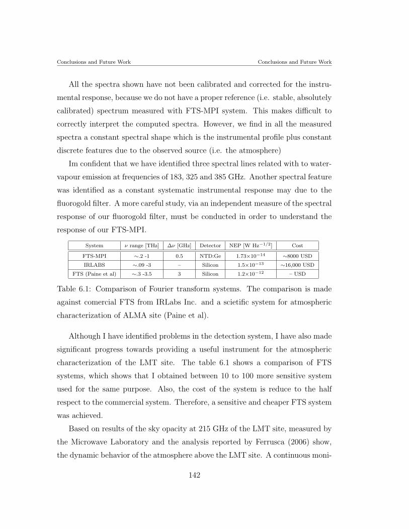
Conclusions and Future Work Conclusions and Future Work
All the spectra shown have not been calibrated and corrected for the instru-
mental response, because we do not have a proper reference (i.e. stable, absolutely
calibrated) spectrum measured with FTS-MPI system. This makes difficult to
correctly interpret the computed spectra. However, we find in all the measured
spectra a constant spectral shape which is the instrumental profile plus constant
discrete features due to the observed source (i.e. the atmosphere)
Im confident that we have identified three spectral lines related with to water-
vapour emission at frequencies of 183, 325 and 385 GHz. Another spectral feature
was identified as a constant systematic instrumental response may due to the
fluorogold filter. A more careful study, via an independent measure of the spectral
response of our fluorogold filter, must be conducted in order to understand the
response of our FTS-MPI.
System ν range [THz] ∆ν [GHz] Detector NEP [W Hz−1/2] Cost
FTS-MPI ∼.2 -1 0.5 NTD:Ge 1.73×10⁻¹⁴ ∼8000 USD
IRLABS ∼.09 -3 – Silicon 1.5×10⁻¹³ ∼16,000 USD
FTS (Paine et al) ∼.3 -3.5 3 Silicon 1.2×10⁻¹² – USD
Table 6.1: Comparison of Fourier transform systems. The comparison is made
against comercial FTS from IRLabs Inc. and a scietific system for atmospheric
characterization of ALMA site (Paine et al).
Although I have identified problems in the detection system, I have also made
significant progress towards providing a useful instrument for the atmospheric
characterization of the LMT site. The table 6.1 shows a comparison of FTS
systems, which shows that I obtained between 10 to 100 more sensitive system
used for the same purpose. Also, the cost of the system is reduce to the half
respect to the commercial system. Therefore, a sensitive and cheaper FTS system
was achieved.
Based on results of the sky opacity at 215 GHz of the LMT site, measured by
the Microwave Laboratory and the analysis reported by Ferrusca (2006) show,
the dynamic behavior of the atmosphere above the LMT site. A continuous moni-
142
Conclusions and Future Work 6.1 Future work
toring of the broadband atmospheric characteristic is therefore necessary in order
to operate the telescope efficiently and establish the various observing strategies
throughout the year (i.e. optimization of the bandpass filtering, telescope time,
engineering time, etc.). In order to continue this effort I describe briefly in the
next section some ideas for improving the current FTS-MPI system, as well a
proposal to design a simple instrument for the LMT.
6.1 Future work
As it has been exposed in this work the Fourier transform spectroscopy has played
an important role in site characterization techniques for determining the sky
transmission spectrum over a wide band (e.g ∼ 215 - 3000 GHz). However this is
not the unique application given to this technique. The Fourier transform spec-
trometers have been used in sub-mm/mm spectroscopy to study planet atmo-
spheres (Weisstein, 1996), FIR studies of complex molecules (Kim & Yang, 1998)
and currently new developments of 2D imaging FTS (Swinyard et al., 2000) as
an example of the this technique. Therefore, we propose to design and develop a
basic Fourier Transform spectrometer as part of the astronomical instruments of
the LMT.
In order to have an spectroscopy instrument for the LMT we need to improve
the current FTS-MPI in order to achieve a high resolution and large S/N in-
strument. These improvements can be achieved following two strategies: i) new
design of the cryogenic detection system and, ii) large throughput interferometer.
6.1.1 He3 bolometric system
A bolometric detection system at He3 (i.e.∼ 300 mK) will inmediately allow us to
improve the performance of the bolometer. A bolometer with a total voltage noise
of 10 nV/Hz1/2 and large responsivity ∼ 109 V/W (i.e. to make the Johnson noise
143
Conclusions and Future Work 6.1 Future work
and amplifier noise contributions negligible), will have a noise equivalent power
on the order of 10−17 W/Hz1/2, which is ∼ 100 times better than we obtained at
1.8 K and the responsivity would also be ∼ 103 times greater.
Operational temperatures < 1 K are just possible using a refrigeration system.
The most common system used is the 4He : 3He closed-cycle fridge which provide
a low microphonic-noise environment, because no mechanical pumps are used.
Also another advantage of these systems is the long hold-times e.g ∼ 72 h, which
require little or no operator intervention, and which in practice is very suitable
for long-time operation of the FTS-MPI system.
A 4He : 3He closed-cycle fridge has two main stages: i) the 4He refrigerator
which pre-cools the heat exchanger to a temperature of 2.7 K to condense the 3He
into the reservoir; ii) and the 3He refrigerator which has a very similar design to
the 4He stage. The vapor pressure of this stage allow us to obtain temperatures
close to 0.3 K.
The complete refrigerator must be installed in a cryostat with the appropriate
dimensions that allow us to allocate the coupling cold-optics and the bolometric
sensor. The required cryostat will have the same configuration as the current
system, with an additional 4.2 K radiation shield that provides a low background
environment to the components (i.e. JFETs, thermometers, heaters, refrigerator,
etc.) installed on the cold-stage.
An example of the system would be the HDL-12 or HDL-14 from IRLABS,
which are 12 and 14 inches cold-plate diameter respectively. The HDL line of
liquid helium dewars contains two cryogenic reservoirs, arranged in the same
mechanical configuration that our cryostat. The cryostat hold-time of this models
are 55 h and 78 h respectively. Custom modifications are possible in order to
accomodate our needs. Figure 6.1 shows the mechanical drawing of the HDL-14.
The cost of the systems are respectively in the range of $ 10,000.00 USD to $20,
000.00 USD for these models.
144
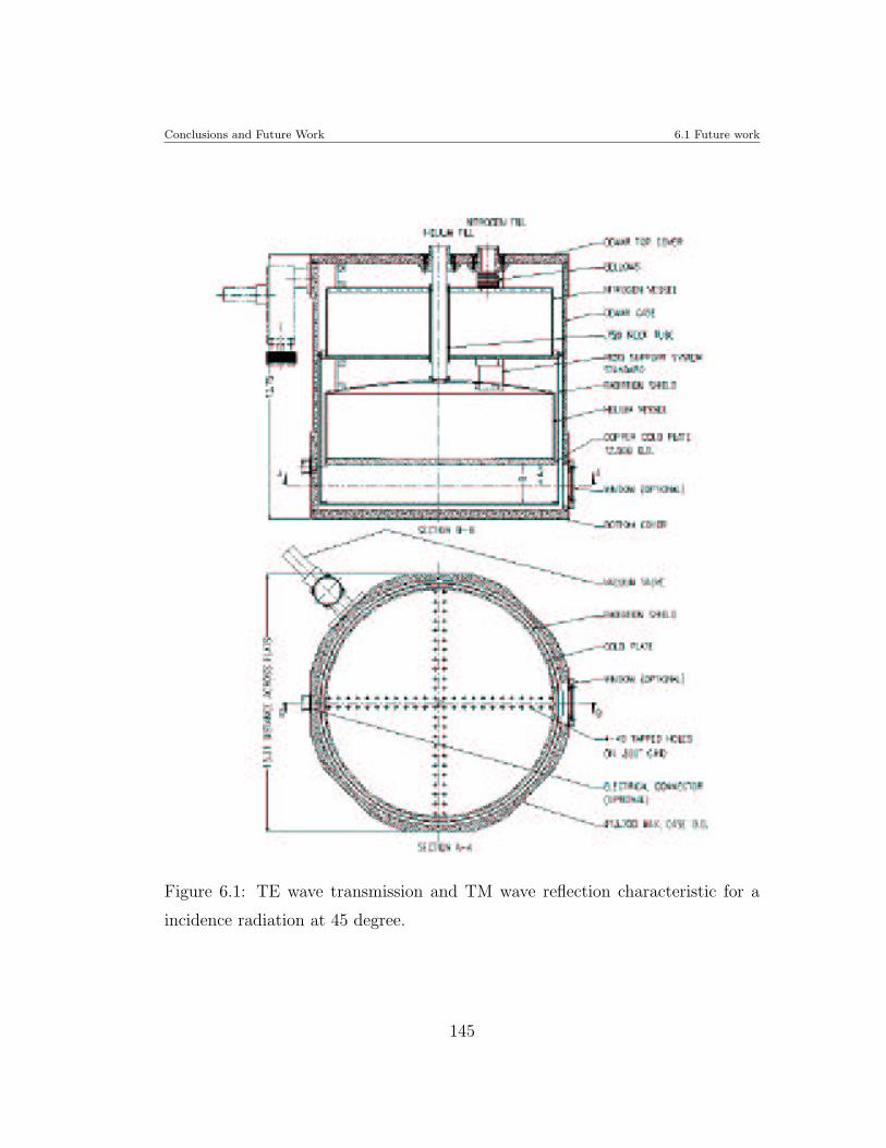
Conclusions and Future Work 6.1 Future work
Figure 6.1: TE wave transmission and TM wave reflection characteristic for a
incidence radiation at 45 degree.
145
Conclusions and Future Work 6.1 Future work
6.1.2 Single pixel or pixel array?
The detection system could be a single pixel or small array. The main objec-
tive in this topic is the choice of the bolometer technology, e.g. silicon nitride
composite bolometers with NTD Ge thermistor or a TES. It does not matter
which technology will be used as long as the final performance parameters will
be improved, such as the thermal conductance, heat capacity and hence the final
NEP, responsivity.
The state-of-the-art in the field of silicon-nitride composite bolometers is rep-
resented by the Spider-Web bolometer. In this technology the absorber is a
metallised silicon-nitride web structure with a small NTD germanium thermistor
bump-bonded to the center. Instruments such as BoloCAM and recently AzTEC
have successfully used these kind of sensors, achieving background-limited per-
formance at temperatures of 100 - 300 mK. BoloCAM at 300 mK reported a
NEP 3 × 10⁻¹⁷ W/Hz1/2 and time constant of 10 ms. This technology could be
explored as the next natural step for future developments at INAOE. In principle
we are able to develop silicon nitride micro-machined structures in cooperation
with the INAOE Department of Electronics. This facility will allow us to start
testing silicon nitride spider-web devices in arrays of a few pixels.
Another investigation topic to be explored in the area of sensor technology is
the use of antenna-coupled microbolometers described by Mees et al. (1991) that
have some attractive features for array applications. These devices use planar
lithographed antennae to coupled the radiation into a thermally active volume.
The advantage of this approach is that the full array can be fabricated onto the
same chip. The ultimate values of NEP are obtained by minimizing the thermal
conductance G, for example G = 9 × 10⁻¹⁰ W/K at 450 mK giving a detector
NEP of 3×10⁻¹⁶ and a time constant of ∼ 0.2 ms. As well as for micro-machined
structures, the planar lithographed antennas can be developed in cooperation
with the Microwave Lab and the Department of Electronics.
146
Conclusions and Future Work 6.1 Future work
No matter which technology we adopt, it is clear that by decreasing the tem-
perature T0 and minimizing the thermal conductance G, of the device we obtain
a considerable gain for the detector responsivity. Therefore these lines of investi-
gation on the silicon spider-web bolometer and TES bolometers will be explored
as future work for the MI-LAB.
6.1.3 Large aperture FTS-MPI system for the LMT
In order to improve the signal-to-noise ratio it is very important to focus all
the efforts toward a large throughput system. This can be achieved by using
larger size optics to provide a large solid angle for collecting the light. The
interferometer will be designed to be mounted at one of the available spaces of
f/10.6 number of the LMT. The size of the beam passing through the system
may be defined in terms of the detector beam, which in principle is modified
by a focusing optics placed at the detector-port aperture-plane. The radiation
entering the interferometer is collimated to reduce the divergence.
I propose to use the same Martin-Puplett interferometer scheme for the FTS.
However we must focus our efforts into producing a better surface quality in all
the optical components. In order to improve the quality of the optics, the opti-
cal surface will be coated with a aluminum to enhance the reflectivity. Another
important issue is to provide a effective method for optical tests at sub-mm/mm
wavelengths that provide information on the final optical quality of optics sys-
tems. To make improvements to the current system and to allow new designs
to be realized we need to implement an alignment tool and aligning process, be-
cause any misalignment introduces phase errors and reduces the fidelity of the
final computed spectrum.
Finally for the rest of the sub-systems (i.e. FTS-control, Data acquisition and
processing software) no great modifications or improvements will be necessary,
since we understand the basics of the FTS spectroscopy, any refinement to the
147
Conclusions and Future Work 6.1 Future work
sub-systems of our 2nd generation FTS will depend on the final application.
To conclude, we have designed, built, integrated and tested a spectroscopic
instrument designed to operate at millimeter wavelength. This experimental de-
velopment has played an important role in the creation of the initial infrastructure
and consolidation of a millimetric wavelength laboratory at INAOE. The Gran
Telescopio Milimetrico (GTM) will rely heavily on the continued development of
this laboratory, its resources and the acquired technical skills. The results from
the initial laboratory tests demonstrate that the FTS will be capable, after im-
provements, of measuring the seasonal variations in the atmospheric transmission
above Sierra La Negra, the site of the GTM.
148
Bibliography
Alpher, R. A., Herman, R., & Gamow, G. A. (1948). Thermonuclear Reactions
in the Expanding Universe. Physical Review, 74, 1198–1199.
Alsop, D. C., Inman, C., Lange, A. E., & Wibanks, T. (1992). Design and
construction of high-sensitivity, infrared bolometers for operation at 300 mK.
Applied Optics, 31, 6610–6615.
Bennett, C. L., Banday, A. J., Gorski, K. M., Hinshaw, G., Jackson, P., Keegstra,
P., Kogut, A., Smoot, G. F., Wilkinson, D. T., & Wright, E. L. (1996). Four-
Year COBE DMR Cosmic Microwave Background Observations: Maps and
Basic Results. Astrophisical Journal Letters, 464, L1+.
Blain, A. W., Smail, I., Ivison, R. J., Kneib, J.-P., & Frayer, D. T. (2002).
Submillimeter galaxies. Physics Reports, 369, 111–176.
Blea, J. M., Parks, W. F., Ade, P. A. R., & Bell, R. J. (1970). Optical Properties
of Black Polyethylene from 3 to 4000 cm-1. Journal of the Optical Society of
America (1917-1983), 60, 603–+.
Chamberlin, R. A., Martin, R. N., Martin, C. L., & Stark, A. A. (2003). Submil-
limeter atmospheric FTS at the geographic South Pole. In Phillips, T. G. &
Zmuidzinas, J. (Eds.), Millimeter and Submillimeter Detectors for Astronomy.
149
Bibliography Bibliography
Edited by Phillips, Thomas G.; Zmuidzinas, Jonas. Proceedings of the SPIE,
Volume 4855, pp. 609-620 (2003)., (pp. 609–620).
Chambers, W. G., Costley, A. E., & Parker, T. J. (1988). Characteristic curves
for the spectroscopic performance of free-standing wire grids at millimeter and
submillimeter wavelengths. International Journal of Infrared and Millimeter
Waves, 9, 157–172.
Coble, K., Dragovan, M., Kovac, J., Halverson, N. W., Holzapfel, W. L., Knox,
L., Dodelson, S., Ganga, K., Alvarez, D., Peterson, J. B., Griffin, G., Newcomb,
M., Miller, K., Platt, S. R., & Novak, G. (1999). Anisotropy in the Cosmic
Microwave Background at Degree Angular Scales: Python V Results. ApJL,
519, L5–L8.
Delgado, G., Otrola, A., & V., B. (2000). The determination of pricipitable
water vapour at llano chajnantor from observations of the 183 ghz water line.
Technical report. NRAO.
Dicke, R. H., Peebles, P. J. E., Roll, P. G., & Wilkinson, D. T. (1965). Cosmic
Black-Body Radiation. Astrophisical Journal, 142, 414–419.
Dragovan, M., Ruhl, J. E., Novak, G., Platt, S. R., Crone, B., Pernic, R., &
Peterson, J. B. (1994). Anisotropy in the microwave sky at intermediate angular
scales. ApJL, 427, L67–L70.
D’yachkov, E. I. (1979). Thermal Conductivity and Electrical Resistivity of NbTi
(HT-50) as fuction of temperature and Magnetic Field . Preprint of the Joint
Institute of Nuclear Research.
Efros, A. L. & Shklovskii, B. I. (1975). Coulomb gap and low temperature con-
ductivity of disordered systems . Journal of Physics C Solid State Physics, 8,
L49–L51.
150
Bibliography Bibliography
Estrada, J., Meza, J., & Torres, A. (2002). Mediciones de opacidad atmosferica en
el volcan sierra negra. Technical report. INAOE/GTM, Tonantzintla, Puebla.,
RT0545.
Ferrusca, D. (2006). A Cryogenic 4He bolometer system for detecting (sub-)-
millimeter wavelength radiation.
Franceschini, A. (2001). The Cosmic Star-Formation History: The Far-IR and
Sub-mm View. In Starburst Galaxies: Near and Far, (pp. 328–+).
Guilloteau, S. (2000). The ALMA Project (Invited Review). In Garzon, G.,
Eiroa, C., de Winter, D., & Mahoney, T. J. (Eds.), ASP Conf. Ser. 219: Disks,
Planetesimals, and Planets, (pp. 645–+).
Hagmann, C., Benford, D. J., Clapp, A. C., Richards, P. L., & Timbie, P. (1992).
A broadband THz receiver for low background space applications. In Michigan
Univ., The Third International Symposium on Space Terahertz Technology:
Symposium Proceedings p 678-687 (SEE N93-27726 10-31), (pp. 678–687).
Haller, E. E., Palaio, N. P., Rodder, M., Hansen, W. L., & Kreysa, E. (1982).
NTD germanium: A novel material for low-temperature bolometers. NASA
STI/Recon Technical Report N, 83, 28412–+.
Halpern, M., Gush, H. P., Wishnow, E., & de Cosmo, V. (1986). Far infrared
transmission of dielectrics at cryogenic and room temperatures - Glass, Fluo-
rogold, Eccosorb, Stycast, and various plastics. Applied Optics, 25, 565–570.
Hughes, D. H. (2005). The Large Millimetre Telescope (LMT): tracing the evo-
lution of structure in the early universe. In Revista Mexicana de Astronomia y
Astrofisica Conference Series, (pp. 97–100).
Hughes, D. H. & Dunlop, J. S. (1999). Continuum Observations of the High-
Redshift Universe at Sub-millimetre Wavelengths. In Carilli, C. L., Radford,
151
Bibliography Bibliography
S. J. E., Menten, K. M., & Langston, G. I. (Eds.), ASP Conf. Ser. 156: Highly
Redshifted Radio Lines, (pp. 99–+).
Hughes, D. H., Serjeant, S., Dunlop, J., Rowan-Robinson, M., Blain, A., Mann,
R. G., Ivison, R., Peacock, J., Efstathiou, A., Gear, W., Oliver, S., Lawrence,
A., Longair, M., Goldschmidt, P., & Jenness, T. (1998). High-redshift star
formation in the Hubble Deep Field revealed by a submillimetre-wavelength
survey. Nature, 394, 241–247.
Ishiguro, M., Kanzawa, T., & Kasuga, T. (1990). Monitoring of atmospheric
phase fluctuations using geostationary satellite signals. In Baldwin, J. E. &
Wang, S. (Eds.), URSI/IAU Symposium on Radio Astronomical Seeing, (pp.
60–63).
Kim, C. & Yang, J. (1998). Quantitative FT-IR Analysis for Chondritic Mete-
orites: Search for C 60 in Meteorites. Journal of Astronomy and Space Sciences,
15, 151–162.
Kooi, J. W., Schaffer, P. L., Bumble, B., Leduc, R., & Phillips, T. G. (1998). Het-
erodyne instrumentation at the CSO. In Phillips, T. G. (Ed.), Proc. SPIE Vol.
3357, p. 22-32, Advanced Technology MMW, Radio, and Terahertz Telescopes,
Thomas G. Phillips; Ed., (pp. 22–32).
Kovac, J., Dragovan, M., Schleuning, D. A., Alvarez, D., Peterson, J. B., Miller,
K., Platt, S. R., & Novak, G. (1997). Anisotropy in the Cosmic Microwave
Background: Results from Python IV. Bulletin of the American Astronomical
Society, 29, 1394–+.
Lamb, J. W. (1993). Infrared filters for cryogenic millimeterwave receivers. In-
ternational Journal of Infrared and Millimeter Waves, 14, 959–967.
Lange, A. E., Hayakawa, S., Matsumoto, T., Matsuo, H., & Murakami, H. (1987).
Rocket-borne submillimeter radiometer. Applied Optics, 26, 401–409.
152
Bibliography Bibliography
Lay, O. P. & Halverson, N. W. (2000). The Impact of Atmospheric Fluctuations
on Degree-Scale Imaging of the Cosmic Microwave Background. ApJ, 543,
787–798.
Lee, S.-F., Gildemeister, J. M., Holmes, W., Lee, A. T., & Richards, P. L. (1998).
Voltage-Biased Superconducting Transition-Edge Bolometer with Strong Elec-
trothermal Feedback Operated at 370 mK. Applied Optics, 37, 3391–3397.
Low, F. J. (1961). Low-Temperature Geranium Bolometer. Journal of the Optical
Society of America (1917-1983), 51, 1300–+.
Mather, J. C. (1982). Bolometer noise: nonequilibrium thoery. Applied Optics,
21, 1125–1129.
Mather, J. C., Hauser, M. G., Bennett, C. L., Boggess, N. W., Cheng, E. S.,
Eplee, R. E., Freudenreich, H. T., Gulkis, S., Isaacman, R. B., & Janssen, M.
(1990). Early results from the Cosmic Background Explorer (COBE). In Liege
International Astrophysical Colloquia, (pp. 25–31).
Matsuo, H., Sakamoto, A., & Matsushita, S. (1998). FTS measurements of
submillimeter-wave opacity at Pampa la Bola. In Phillips, T. G. (Ed.), Proc.
SPIE Vol. 3357, p. 626-637, Advanced Technology MMW, Radio, and Terahertz
Telescopes, Thomas G. Phillips; Ed., (pp. 626–637).
Matsushita, S., Matsuo, H., Pardo, J. R., & Radford, S. J. E. (1999). FTS
Measurements of Submillimeter-Wave Atmospheric Opacity at Pampa la Bola
II : Supra-Terahertz Windows and Model Fitting. PASJ, 51, 603–+.
Matsushita, S., Matsuo, H., Sakamoto, A., & Pardo, J. R. (2000). FTS mea-
surements of submillimeter opacity and other site testing at Pampa la Bola.
In Butcher, H. R. (Ed.), Proc. SPIE Vol. 4015, p. 378-389, Radio Telescopes,
Harvey R. Butcher; Ed., (pp. 378–389).
153
Bibliography Bibliography
Mauskopf, P. D., Bock, J. J., del Castillo, H., Holzapfel, W. L., & Lange, A. E.
(1997). Composite infrared bolometers with Si 3 N 4 micromesh absorbers.
Applied Optics, 36, 765–771.
Mees, J., Nahum, M., & Richards, P. L. (1991). New designs for antenna-coupled
superconducting bolometers. Applied Physics Letters, 59, 2329–2331.
Mertz, L. (1965). Transformations in Optics. New York: John Wiley & Sons,
Inc.
Nishioka, N. S., Richards, P. L., & Woody, D. P. (1978). Composite bolometers
for submillimeter wavelengths. Applied Optics, 17, 1562–1567.
Penzias, A. A. & Wilson, R. W. (1965). A Measurement of Excess Antenna
Temperature at 4080 Mc/s. Astrophisical Journal Letters, 142, 419–421.
Platt, S. R., Kovac, J., Dragovan, M., Peterson, J. B., & Ruhl, J. E. (1997).
Anisotropy in the Microwave Sky at 90 GHz: Results from Python III. ApJL,
475, L1+.
Puget, J. L., Lagache, G., Clements, D. L., Reach, W. T., Aussel, H., Bouchet,
F. R., Cesarsky, C., Desert, F. X., Dole, H., Elbaz, D., Franceschini, A., Guider-
doni, B., & Moorwood, A. F. M. (1999). FIRBACK. I. A deep survey at 175
microns with ISO, preliminary results. Astronomy and Astrophysics, 345, 29–
35.
Richards, P. L. (1994). Bolometers for infrared and millimeter waves. Journal of
Applied Physics, 76, 1–24.
Ruhl, J. E., Dragovan, M., Platt, S. R., Kovac, J., & Novak, G. (1995). Anisotropy
in the Microwave Sky at 90 GHz: Results from Python II. ApJL, 453, L1+.
Sanders, D. B. & Mirabel, I. F. (1996). Luminous Infrared Galaxies. Annual
review of astronomy and astrophysics, 34, 749–+.
154
Bibliography Bibliography
Saunders, W., Rowan-Robinson, M., Lawrence, A., Efstathiou, G., Kaiser, N.,
Ellis, R. S., & Frenk, C. S. (1990). The 60-micron and far-infrared luminosity
functions of IRAS galaxies. Royal Astronomical Society, Monthly Notices, 242,
318–337.
Scott, D., Borys, C., Chapman, S. C., Donahue, M., Fahlman, G. G., Halpern, M.,
& Newbury, P. (2002). A giant sub-mm lensed arc? Bulletin of the American
Astronomical Society, 34, 1312–+.
Serlemitsos, A. T. (1989). Flight worthy infrared bolometers with high through-
put and low NEP. In Melugin, R. K. & Pierce, W. G. (Eds.), Cryogenic optical
systems and instruments III; Proceedings of the Meeting, San Diego, CA, Aug.
17-19, 1988 (A90-11251 01-31). Bellingham, WA, Society of Photo-Optical In-
strumentation Engineers, 1989, p. 314-321., (pp. 314–321).
Smail, I., Ivison, R. J., & Blain, A. W. (1997). A Deep Sub-millimeter Survey
of Lensing Clusters: A New Window on Galaxy Formation and Evolution.
Astrophisical Journal Letters, 490, L5+.
Soifer, B. T., Neugebauer, G., & Houck, J. R. (1987). The IRAS view of the
extragalactic sky. Annual review of astronomy and astrophysics, 25, 187–230.
Swinyard, B. M., Ade, P. A., Griffin, M. J., Dohlen, K., Baluteau, J.-P.,
Pouliquen, D., Ferand, D., Dargent, P., Michel, G., Martignac, J., Rodriguez,
L., Jennings, D. E., Caldwell, M. E., Richards, A. G., Hamilton, P. A., &
Naylor, D. A. (2000). FIRST-SPIRE spectrometer: a novel imaging FTS for
the submillimeter. In Breckinridge, J. B. & Jakobsen, P. (Eds.), Proc. SPIE
Vol. 4013, p. 196-207, UV, Optical, and IR Space Telescopes and Instruments,
James B. Breckinridge; Peter Jakobsen; Eds., (pp. 196–207).
Torbet, E., Devlin, M. J., Dorwart, W. B., Herbig, T., Miller, A. D., Nolta, M. R.,
Page, L., Puchalla, J., & Tran, H. T. (1999). A Measurement of the Angular
155
Bibliography Bibliography
Power Spectrum of the Microwave Background Made from the High Chilean
Andes. ApJL, 521, L79–L82.
Torres, V., Davydova, V., Carrasco, L., & Guzmn, I. (1997). Evaluation of the
long term behaviour of sites for mm-wavelength radioastronomy: the quest
for a site for the large millimeter telescope. Technical report. INAOE/GTM,
Tonantzintla, Puebla., Dic.97.
van Vleck, J. H. (1947a). The Absorption of Microwaves by Oxygen. Physical
Review, 71, 413–424.
van Vleck, J. H. (1947b). The Absorption of Microwaves by Uncondensed Water
Vapor. Physical Review, 71, 425–433.
Weisstein, E. W. (1996). Millimeter/submillimeter Fourier Transform Spec-
troscopy of Jovian Planet Atmospheres. Ph.D. Thesis.
156
List of Figures
1.1 Voltage output of one pixel of the AzTEC camera at 1.1 mm, look-
ing at the sky above Mauna Kea. The top panel shows the sky vari-
ations over a times-scale of 1 minute. The two curves show mea-
surements taken under different sky opacity conditions(τ215GHz ∼0.034, dark-line; τ215GHz ∼ 0.114, red-line). The bottom panel
shows the power-spectrum density of the sky under the opacity
conditions shown in the upper panel, where the dark-line and red-
line again represent low and high opacity conditions. . . . . . . . 3
157
List of Figures List of Figures
1.2 Top panel: The COBE image shows the reduced map (i.e., both the
dipole and Galactic emission subtracted). The cosmic microwave
background fluctuations are extremely faint, 10 µK compared to
the 2.73 K average temperature of the radiation field. Bottom
panel: The later WMAP image shows a higher resolution image of
the CMB temperature fluctuations of ∼ 1 µK. The CMB radiation
is a remnant of the Big Bang and the temperature fluctuations are
evidence of variations in the density of the early universe. These
density ripples are believed to have given rise to the largest struc-
tures that populate the universe today, i.e. clusters of galaxies and
vast regions devoid of galaxies. . . . . . . . . . . . . . . . . . . . . 7
1.3 Flux density of a ULIRG (e.g. Arp 220) as a function of the red-
shift. The flux density is observed at wavelengths of 175, 450 and
850 µm, over a range of redshifts z = 0.1− 10. The lines of differ-
ent thickness illustrate 20 K, 40 K and 80 K SED temperatures.
The graphs were made using a pure evolution model (i.e. 5× 10¹²,
β = 1.5, Ωo = 0.3 and ΩΛ = 0.7). As the SED is redshifted, it be-
comes fainter, but the negative k-correction compensates for this
dimming, and so the flux remains basically constant for z ∼ 1 − 8
(e.g. at 850 µm wavelength). In the case of longer wavelengths
or warmer SEDs, the k-correction increases the observed flux at
higher redshifts. . . . . . . . . . . . . . . . . . . . . . . . . . . . . 9
158
List of Figures List of Figures
1.4 The three main components of the extragalactic background spec-
trum. The dominant component is the microwave background at
millimetric wavelengths given by the primordial Universe at the
epoch of recombination. The second component is the FIR/sub-
mm/mm background produced by galaxies in the young Universe,
and finally the third component is the IR/optical background due
to the light coming from stars, galaxies and AGN in the evolved
Universe. (Busswell & Shanks, adapted by Holland et al. 2004) . 11
1.5 Synthetic atmospheric spectrum of the sky at La Negra for 1 mm
PWV (using the ATM code). . . . . . . . . . . . . . . . . . . . . 14
1.6 Stratification of the Earth atmosphere showing the change in tem-
perature (K) with the increasing altitude (km). . . . . . . . . . . 16
1.7 Rotational energy level diagram for water-vapour (Guelin, 1998). . 17
1.8 215 GHz opacity for the LMT site, measured during 1997-2002.
The best season for sub-mm/mm observation are from November
through May with opacity values < 0.2. Data reduction by Mi-
crowave Laboratory, INAOE . . . . . . . . . . . . . . . . . . . . . 21
1.9 Simulated atmospheric transmission spectrum for the LMT site.
The black solid-line and red dashed-line illustrate the atmospheric
model for winter and summer mean opacity respectively (1997-
2004). The blue dot-dashed line is the measured AzTEC bandpass
(∼ 1.1mm). The gray dot-dashed lines illustrate the central fre-
quency bandpasses of the SPEED camera (SPEctral Energy Dis-
tribution camera) . . . . . . . . . . . . . . . . . . . . . . . . . . . 23
1.10 Fourier Transform Spectrometer in the MI-LAB, INAOE, showing
the FTS-MPI (front-right), the cryostat (back-left) and associated
electronics. . . . . . . . . . . . . . . . . . . . . . . . . . . . . . . . 25
2.1 The sinc function convolved with a single spectral line at σ1. . . . 35
159
List of Figures List of Figures
2.2 Spectrum replication and sampling rate: a) the correct choice of
the sampling rate produces an spectrum confined to one-half of the
replica period; b) a bad selection of the sampling rate will produce
an overlap of the replicated spectrum. . . . . . . . . . . . . . . . . 37
2.3 A schematic of a Martin-Puplett interferometer, showing the posi-
tion and orientation of the various ports, mirrors an and polarizing
grids. . . . . . . . . . . . . . . . . . . . . . . . . . . . . . . . . . . 41
3.1 At the left the resistance versus temperature characteristic for a
superconducting Ti film at Tc∼370mK (Lee et al., 1998). At the
right the voltage-biased bolometer with the SQUID read-out am-
plifier. . . . . . . . . . . . . . . . . . . . . . . . . . . . . . . . . . 48
3.2 Schematic principle of operation . . . . . . . . . . . . . . . . . . . 49
3.3 Typical bias circuit for a single bolometer represented as a variable
resistor Rbol . . . . . . . . . . . . . . . . . . . . . . . . . . . . . . 51
3.4 R-T curves for diferents NTD:Ge thermistors from Haller-Beeman
Inc. The thermistor type B was selected to build the bolometer
for the detection system. . . . . . . . . . . . . . . . . . . . . . . . 59
4.1 Details of the composite bolometer unit. . . . . . . . . . . . . . . 62
4.2 Bolometer unit details. The bolometer unit is suspended at the
center of a brass ring by two nylons string that provide mechan-
ical support. The two copper leads are connected to the 12 µm
diameter NbTi leads that allows the electrical connection to the
amplification stages. . . . . . . . . . . . . . . . . . . . . . . . . . 63
4.3 Thermal conductivity model for NbTi. The data shown with trian-
gles are the experimental values reported in literature. The solid-
line is model for a temperature range ∼1.5 - 8 K. The vertical
dotted-lines shows the temperature range used for the bolometer
characterization. . . . . . . . . . . . . . . . . . . . . . . . . . . . 67
160
List of Figures List of Figures
4.4 Modified experimental dewar from Oxford Instruments. Inc. The
dewar is a liquid helium system with vapor-cooled and liquid ni-
trogen shields. . . . . . . . . . . . . . . . . . . . . . . . . . . . . . 71
4.5 Cool down process chart of the different stages of the cryostat. The
JFET is maintained at about 120 K using a heater. . . . . . . . . 73
4.6 Cooling-down process during the liquid helium transfer stage. . . 74
4.7 Modified configuration of the cold optics, to provide greater tem-
perature stability of the bolometer and feed-horn. . . . . . . . . . 76
4.8 Cooling-down process. Base plate behavior during the cooling with
the liquid helium transfer. . . . . . . . . . . . . . . . . . . . . . . 77
4.9 The bolometer schematic circuit for biasing and readout. The gray
boxes show the different temperature stages. . . . . . . . . . . . . 79
4.10 Schematic circuit of the warm amplifier stage. The stage composed
with the AD624AD is the differential amplification stage which is
coupled to a bi-quad bandpass filter builded with the OP470Y
operational amplifier. . . . . . . . . . . . . . . . . . . . . . . . . . 80
4.11 Transmission characteristic for materials used for FIR/IR filters
in the detection system camera. The red-dashed line is the model
for fluorogold transmission with a thickness of ∼1.25 mm (Halpern
et al., 1986); the circle data shows the transmission characteristic
of the black-polyethylene (Blea et al., 1970); the solid line is a
modified data of the Zotefoam losses reported by Kooi et al. (1998). 82
4.12 Winston cone geometry. The field of view is defined by the accep-
tance angle θ, which depends on the total length of the cone and
on the diameter of the entrance and exit apertures. . . . . . . . . 84
4.13 Inside view of the base plate of the criostat with the coupling optics
and the IR-blocking filtering mounted in place. . . . . . . . . . . . 86
4.14 Synthetic voltage-current characteristic (load-curve) obtained us-
ing the model parameters in table 4.3, for temperature of 1.8 K. . 89
161
List of Figures List of Figures
4.15 Responsivity vs. current obtained from the synthetic load-curve
shown in Figure 4.14, for a temperature of 1.8 K . . . . . . . . . . 90
4.16 Noise Equivalent Power (NEP) vs. current, obtained from the
synthetic load curve at T0=1.8 K, the low bias regime was removed
from the plot for clarity. . . . . . . . . . . . . . . . . . . . . . . . 91
4.17 The bolometer block diagram for biasing and readout electronics.
The bias current is obtained by measuring the Vbol at different
values of Vbias. . . . . . . . . . . . . . . . . . . . . . . . . . . . . 92
4.18 Load-curves set, for different bath temperatures: i) cross-blue line
4.14 K; ii) dotted-green line 3 K; iii) plus-red line 2.5 K; iv) circle-
green line 2 K. . . . . . . . . . . . . . . . . . . . . . . . . . . . . . 94
4.19 Log(R) vs. 1/T 1/2 characteristic. The diamond points show the
expected data from Haller type B thermistor; the triangle points
show the experimental data for which R0 = 25412.59 [Ω] and Tg =
57.50 [K] were obtained. . . . . . . . . . . . . . . . . . . . . . . . 95
4.20 Measured responsivity vs. bias current for a bath temperatures
of 1.9 K (green-circle line) and 4.05 K (blue-triangle line). The
vertical-dashed line shows the operation point used for comparinson. 97
4.21 Total noise equivalent power vs. bias current, for different bath
temperatures. Green-circles show NEP vs. Ibias at 1.9 K. The
blue-triangles show the NEP vs. Ibias at 4.1 K. Operation point is
shown with the vertical-dashed line. . . . . . . . . . . . . . . . . . 98
5.1 TE wave transmission and TM wave reflection characteristic for a
incidence radiation at 45 degree. . . . . . . . . . . . . . . . . . . . 104
5.2 The 140 mm diameter tungsten wire-grid polarizer used as beam
splitter for the FTS-MPI. Installed on aluminum mount. . . . . . 105
5.3 Off-axis parabolic mirror machining at CNC machine. The ma-
chine grooves are still visible after the first cut. . . . . . . . . . . 109
162
List of Figures List of Figures
5.4 A 127 mm diameter, f/4.7 off-axis parabolic mirror showing the
final surface quality. . . . . . . . . . . . . . . . . . . . . . . . . . . 109
5.5 Mylar beam-splitter, held in a 140 mm diameter aluminum ring,
used for the aligning process. . . . . . . . . . . . . . . . . . . . . . 110
5.6 Power spectrum of the local atmosphere derived from the ATM
code for 11 mm of PWV and ∼5 GHz of resolution. . . . . . . . . 111
5.7 Simulated interferogram, obtained from transmission spectrum of
the atmosphere derived from the ATM code, shown in figure 5.6. . 112
5.8 Power spectrum (solid-line) obtained by inverse FFT of the sim-
ulated of the real part of the interferogram in figure 5.7, which
results in reduced signal strength. The dotted-line is the atmo-
spheric power spectrum convolved with the fluorogold transmission
characteristic. . . . . . . . . . . . . . . . . . . . . . . . . . . . . . 113
5.9 Power spectrum deconvolved with the fluorogold transmission cha-
racteristic (solid line). The original spectrum is also shown for
comparison (solid-gray line). . . . . . . . . . . . . . . . . . . . . . 114
5.10 Simulated interferogram (i.e. atmosphere convolved with the flu-
orogold characteristic) plus normally distributed noise in oder to
introduce asymmetries and reduce the S/N ratio. . . . . . . . . . 115
5.11 Recovered power spectrum from the noisy interferogram (i.e. Fig.
5.10 recovered (solid-line). The gray-line is the power spectrum
which was obtained from the ATM code convolved with the fluo-
rogold characteristic. . . . . . . . . . . . . . . . . . . . . . . . . . 116
5.12 Power spectrum from noisy interferogram deconvolved with the
fluorogold transmission characteristic (solid-line). The original at-
mospheric power spectrum shown for comparison (gray-line). . . . 118
5.13 Schematic setup of the first experiment with FTS-MPI. P1 is the
input polarizer; BS is a polarizer used as beam-splitter; P2 is the
output polarizer. . . . . . . . . . . . . . . . . . . . . . . . . . . . 119
163
List of Figures List of Figures
5.14 Top panel: Interferogram record which shows large spikes due to an
unlocked signal events. These events are related to a bad reference
signal generation. Bottom panel shows the PDS of the interfero-
gram record. . . . . . . . . . . . . . . . . . . . . . . . . . . . . . . 120
5.15 Interferogram record showing the voltage drift present in all the
interferograms recorded in the original setup of the FTS-MPI. . . 122
5.16 Various interferograms used to improve the S/N ratio. The top-
left panel shows the set of 4 interferograms used to calculate the
average of those interferograms obtained with the original experi-
mental setup shown in Figure 5.13. Top-right panel shows a detail
of the central region of the individual interferograms. Bottom-left
panel is the average of the 4 interferograms and bottom-right is a
detailed view of the central region of the average interferogram. . 124
5.17 Computed spectra obtained after inverse Fourier transforming the
average from 5 interferograms set which represent different hours
during day in which the experiment was conducted (from the morn-
ing to evening). . . . . . . . . . . . . . . . . . . . . . . . . . . . . 125
5.18 Current configuration of the FTS-MPI. . . . . . . . . . . . . . . . 127
5.19 Interferogram recorded using step-integrate mode, looking the sky. 128
5.20 Signal to noise ratio of the interferogram. The dotted line shows
the required level of the S/N ratio. . . . . . . . . . . . . . . . . . 129
5.21 Position vs. time of the central bright fringe. Top-panel data
obtained using liquid nitrogen as a source. Middle-panel data ob-
tained looking at the sky. Bottom-panel data obtained using a
variable blackbody source. . . . . . . . . . . . . . . . . . . . . . . 130
5.22 Set of measured interferograms obtained in the last run experi-
ment. The FTS-MPI system was illuminated with the sky power
signal and referenced with liquid nitrogen sources. . . . . . . . . . 132
164
List of Figures List of Figures
5.23 Computed power spectra from the measured interferograms shown
in Figure 5.22. From the top, the first three panels show the
computed spectra from single interferogram record, the last panel
shows the average of 5 spectra. . . . . . . . . . . . . . . . . . . . 133
5.24 The solid dark line is the computed spectrum from 5 spectra average.
The solid gray line shows a single computed spectrum which is also for
comparison. . . . . . . . . . . . . . . . . . . . . . . . . . . . . . . 135
5.25 Similar to the figure 5.24 the solid dark line is the computed spectrum
from 10 spectra average process. . . . . . . . . . . . . . . . . . . . . 135
5.26 Average spectra for different stages of the experiment during the
day. The top panel is the average of 10 spectrum from measured
interferograms recorded during the morning. The middle panel is
the average of 10 spectrum for noon and the bottom panel is the
average spectrum for the evening. . . . . . . . . . . . . . . . . . . 136
5.27 Average spectrum from full set of interferograms obtained in the
experimental run observing the sky (solid-dark line). The 183 GHz
water-vapour line and 380, 382, 386 390 and 391 GHz water-vapour
blend lines. The vertical-dotted lines show the position of the
central frequency of the measured lines. . . . . . . . . . . . . . . . 138
6.1 TE wave transmission and TM wave reflection characteristic for a
incidence radiation at 45 degree. . . . . . . . . . . . . . . . . . . . 145
165

List of Figures List of Figures
166
List of Tables
3.1 NEP performance for NTD:Ge composite bolometers at different
bath temperatures. . . . . . . . . . . . . . . . . . . . . . . . . . . 56
4.1 Bolometer dimension, heat capacity and thermal conductance . . 70
4.2 Parameter used for model bolometer . . . . . . . . . . . . . . . . 83
4.3 Parameters used for bolometer model in simulated V-I curves. . . 88
5.1 Dimesion of the f/4.8 Winston cone. . . . . . . . . . . . . . . . . 107
6.1 Comparison of Fourier transform systems. The comparison is made
against comercial FTS from IRLabs Inc. and a scietific system for
atmospheric characterization of ALMA site (Paine et al). . . . . . 142
167