Embed Size (px)
Citation preview

JOURNAL OF MATHEMATICAL ANALYSIS AND APPLICATIONS 26, 479-511 (1969)
A Poisson Integral Formula for Solutions of Parabolic Partial Differential Equations*
JEFF E. LEWIS
University of Illinois at Chicago Circle, Chicago, Illinois 60680
Submitted by Peter D. Lax
1. INTRODUCTION
The algebra of pseudo-differential operators has been utilized by Calderon [3] and Seeley [14] to construct a projector onto the space of bound- ary values of solutions of elliptic partial differential equations. KreC [I I] has suggested a generalization of the algebra of pseudo-differential operators of Kohn and Nirenberg [lo] to include the parametrix of a parabolic operator. We here employ this algebra of quasi-homogeneous pseudo-differential operators to consider the lateral boundary values of solutions of the parabolic differential equation
Au = C a, D,h - in G’ = [0, T) x sZ+, IwGm
u(0, x) = 0, XEQ+. (l-1)
If u is smooth define R,u to be its Cauchy data of order < m on the lateral boundary X = [0, T) x AQf. If u is a solution of (1.1) and is assumed only to be a distribution on [0, T) x closure Q+, we will show the validity of a Poisson integral representation for u in terms of ROu (defined as lim,+,,+ Cauchy data on the surface dist((t, x), X) = l ). In particular R,,u exists, and we may obtain a priori estimates, even though we cannot rely on a trace lemma.
The function spaces which arise in the study of parabolic equations have different smoothness in the spatial variables than in the time variable; Sobolev spaces which describe this property are introduced in Section 2. In Section 3 we specialize to the “parabolic case”. Lemma 3.10 will be impor-
* This paper was written while the author was a visiting member at the Courant Institute of Mathematical Sciences, New York University, and revised under N.S.F. Grant number GP-8289.
479
brought to you by COREView metadata, citation and similar papers at core.ac.uk
provided by Elsevier - Publisher Connector

480 LEWIS
tant in the proofs that follow. Here we also make precise the initial condition u(0, x) = 0.
The properties of the quasi-homogeneous pseudo-differential operators which act on the spaces of Section 2 are considered in Section 4; we also define the operators on products of Cm manifolds. The reader famihar with the properties of the usual pseudo-differential operators, particularly as developed in ([El, Chapter 16) will be content to look at the definitions and statements in this section.
The parabolic differential operator is introduced in Section 5; Theorems 5.6 and 5.7 are the main results of the paper. The main result may be described as follows.
If ST is the strip [0, 2’) x Rn and s is a positive integral multiple of m, let &(Sr) be those functions u with D,jD,eu ELM for mj + 1 /3 1 < s and ~(0, x) = 0; the space fi-s(S,) is the dual of {U : D,iD,eu eL2(ST), mj + 1 p 1 < s and u(T, x) = O]. Let &(X) = @;I”-’ fiR-+liz(X). Let
&(A, s) = {u E I&(&-) : Au = 0 in G+}.
THEOREM. For all real s, R, is continuous from &A, s) into l%(X). There is a continuous map P from &(X) onto &(A, s) such that P+ = R,P is a pro-
jection onto R,(&(A, s)).
The operators P (called the Poisson integral) and Pf are defined in Sec- tion 6. The basic lemmas follow the outline of Seeley [14] for the elliptic case.
The second main theorem (5.7) is proved in Section 7. Section 8 summarizes other papers on the problem (1.1) and related
problems.
2. DESCRIPTION OF SOME FUNCTION SPACES
For x = (x1 ,..., x,), 5 = (h ,..., &) E R” let Zp!i xi& be denoted by x * 5 or x[ and 1 x 1 = (x * x)1/2. Let 01 = (cyr ,..., ar,) be a fixed n-tuple of positive numbers and define 1 (Y 1 as a, + *em + OL, . For h > 0 and 3c E R” let
TX = (A%, ,..., Px,) and A-“x = (A-‘)” x.
We shall call a function on RQ N (0) q uasi-homogeneous of degree r if f(A”x) = #‘j(x) for all X > 0, x + 0. We shall consider Rn equipped with a Cm metric p(x) which is quasi-homogeneous of degree 1 and let dist(x, y) = p(x - y). For example [6] let p(x) be the unique number p such

POISSON INTEGRAL FORMULA 481
that g(x, p) = C ~$/p~~i = 1. Th ere is a natural polar coordinate system associated with p so that for f E C*
(2.1)
Here da is the Lebesgue measure on the unit sphere Z and
1 < J(u) < max oli .
Let Dj = (- is/ax,) and for /3 = (PI ,..., /3J an n-tuple of nonnegative integers let 39 = x9 *** ~2. The space Y is the space of tempered functions and ,Y’ its conjugate dual. For f E 9 define its Fourier transform by f*(t) = J” e-isEf(x) d x and for T E Y’ let TA be defined by (f, T^) = <f^, T).
We now introduce a Bessel potential operator. For s real let
G”(f) = (1 + p(V-“‘“.
Then if f A is a locally integrable function define Asf by
(AW(E) = GV)f%). (2.2)
DEFINITION 2.3. By H,S(R”) we denote the isometric image of L2(Rn) = H,O(R”) under AS.
The Hilbert space norm on H,8(R”) is given by
II u II:;;, = (2J7Y j (1 + p(f)“)” I W) I2 d5.
For s > 0, u E II&~(R”) means approximately that Deu E L2 for
/I * 01 = ‘q&c+ < s.
(2.4)
The spaces Ha8(R”) and H;“(R”) are conjugate duals under the sesquilinear form
(u, v) = 1 u(x) v(x)* dx for U,VEY. (2.5)
Here v* is the complex conjugate of v.
LEMMA 2.6. The collection {H,8(R”)},,, is a continuous chain of Hilbert spaces and in fact a scale (see Palais [12], p. 141).
COROLLARY 2.7. Let T : 9 + Y be a linear operator such that
II Tf lls<:a = ci Ilf /I*i;a P i = 1,2.

482 LEWIS
ForO<B<l,Zetp(B)=Bp,+(l--)p,,9(8)=89,+(1--)q,. Then
DEFINITION 2.8. A linear operator T : Y--f 9’ is of order < Y (or T E Op, - a) if and only if for every s, there is a constant C = C(s) such that
II Tflls:, < C Ilfllstr;a -
The true order of T is inf(r : T E Op, - a>. The space of operators of true order - co is denoted by Op-, - 01.
Of course T E Op, - 01 if and only if A-“T /h\a+r is a bounded operator on L2 for every s.
The Sobolev lemma to be used in the sequel is
LEMMA 2.9. For k > I a l/2, H,“(R”) C CO(R”) and the injection is con- tinuous.
3. SOBOLEV SPACES FOR THE STUDY OF
PARABOLIC PARTIAL DIFFERENTIAL EQUATIONS
To use the standard notations of parabolic partial differential equations, we assume that our operators are defined on functions of (n + 1) variables with x1 = t a time variable and x = (x2 ,..., x~+~) an n-dimensional space variable and write points as (t, X) with dual variables (7, t). Let 01 = (01~ , (Y’) with 0~~ = m, an even integer, and a2 = *a* = 01,+~ = 1.
DEFINITION 3.1. The space fiaS(Rt+l) is
(24 E H,“(RRnf’) : supp u c ((t, X) : t > 0)).
We next consider the parabolic Bessel potential operator A8 defined by
(hsf)^ (7, 5) = (1 + I E lm + i+“‘“f^(T, 0. (3.2)
Then
supp SsfC (t > a> if suppff (t 3 u>. (3.3)
If II E L2(Rz+1), consider u E H,O(P+r) by extending u to be zero for t < 0.
LEMMA 3.4. The distribution u E I&“(Rf+l) if and only if u = Ay where
f E L’(Rz’l) and c,-‘II u IL < llf I10 G c, II u ll8:o -

POISSON INTEGRAL FORMULA 483
PROOF. If f EL~(R:+‘), A-8(Ay) E H”(Rn+l) and
and
Ay = A”(A+Ay) E Iy(Rnf’)
Conversely, if u E &“(li~+‘), then u = A%, v EL~(P+‘) and
f = A-% E L2(R”=l) and MO G G II v II0 = cs II 24 IL:.. *
For 0 < T < co, let S, = [0, T) x Rn.
DEFINITION 3.5. The space as(&) is
(U : there exists u” E Z&‘(Rt+‘), u” I+ = u>,
equipped with the norm
II 21 IIs3 = inf II 2-i IL . (3.6)
If f ELM, consider f sL2(Rn+l) by extending f to be zero outside ST.
LEMMA 3.7. The distribution u E @S,) ;f and only if u = Ay where
f EL2(ST) and CL’ II u ILT d II f II0 < c.4 II u IIs3 -
PROOF. If f eL2(ST),
ii = h”fe fim3(R:+‘) and 22 Jsr = u E P&)
and II ZJ Ils:T < II ~Yll,:, G C8 Ilf II0 *
Conversely, let u E fig(&) and Ei: E Z?m8(R:+1) be such that u’ I+ = u. Then
f- = A-% E L2(Ry+l) *
and - II u IIa;a 2 c II f II0 2 c II f IILB(ST) -
Let f = J in ST, f = 0 outside ST. Then II u IlszT > C II f Ilo and in ST, my=AyJ=li=u. Q.E.D.
The adjoint of A8 is A** defined by
(h8*g)^(7, 5) = (1 + I 5 Im - iT)-g’mgh(T, 5).

484 LEWIS
Let @y&s,) = AS”L2(Sj”).
LEMMA 3.8. The dual space of f@(S,) is I+ under the sesquilinear form
(u, v) = j j,, u(t, x) v*(t, x) dt dx
f OY
u E C;((O, T] x R”), v E C;([O, T) x R”).
PROOF. We first show that [@(&)I* C @-“(ST). If 1 (u, T) 1 < C /I u &:r, let u = Asf, f ELM, and define L : L2(S,)+ C by L(f) = (A$ T). Then we have a g E L2(S,), with ]I g (]L2(sr) < C and a sequence {g,} C Cc([O, T) x Rs) such that g, +g in L2(S,), and for f E Cc((O, T] x R”)
L(f) = jj f(t,x)&x)dtdx ST
= lim JJ‘ f (t, x) g,*<t, 4 dx dt
pf’
= lim TI-SC il
Ay(t, x) (A-“*g,J* dx dt p+1
= (A$ A-S*g) = (Agf, T).
Hence [&(S,)J * C @-“(S,) and the injection is continuous. Let v E@-+(&) n C:(&.). Then if u E C~((O, T] X R”),
II uv* =
and , jj,;L*,
j I,,,, @-"*A* = j j,, A-% g*
< c II A-% 110 II g II0 G c II u lls:Tll ‘u L *
Hence
v E vw%“)l* and sup Iri uv* : II u IL:?- = 11 < c II v IlL *
For k a nonnegative integer, we have another characterization of fik”(Sr).
LEMMA 3.9. The space fikm(S,) is the closure of
D, = (y E Y : fp(t , x) = 0 near t = 0)

POISSON INTEGRAL FORMULA 485
in the norm
PROOF. Since I!-~” = (1 + (- J1”12 - a/8t)k, I v /km and )I v Ijkm:r are equivalent. If u E lTpkm(ST), u = A ““f, where f E L2(Sr). Let (jj} _C D, , fj --t f in L2(Sr). Then p)j = Akmfj + u in fik”(Sr) and {IJJ~} _C D, by (3.3).
We now give a lemma which enables us to prove estimates for operators on the spaces &(Sr) by using estimates for the operators on the spaces &~(Rn+l) (which are easy to obtain by considering certain operators as quasi- homogeneous pseudo-differential operators). The proof is obvious from definition (3.5).
LEMMA 3.10. Let L : Y(P+l) + 9’(Rn+l) be such that
II Lu IL < c II u IL * Suppose that for every real a
supp Lu C {t 3 a} if supp u c {t > Q}.
Then II Lu lls;T G c II u IL,?- *
(3.11)
In the study of boundary value problems we shall need to consider the values of functions restricted to hyperplanes. For u(t, x) E Y(R”+l), let
R1p(t, x’) = u(t, x’, 6). (3.12)
Here (t, x) = (t, xs ,..., x,,,), x’ = (xs ,..., x,). The following trace lemma is an easy consequence of Theorem 2.2.8 in Hormander’s book [8].
LEMMA 3.13. For s > 01,+,/2
is continuous with bounds independent of l . Here 0~’ = (q ,..., 01,).
DEFINITION 3.14. Fork an integer > 0 define for u(t, x) E Y(Rn+l)
Rkru = u(t, x’, <) 0 Dn+lu(t, x’, <) @ +.. @ D;;;u(t, x’, E)). (3.15)
Againletol, = m;ct, = *** = aa+1 = 1. Clearly R,, satisfies (3.11). Hence if
k-l
S; = [0, T) x R”-1 and B,s(S&) = @ fP-l’2(s$) j=o
we have R,, : &(S,) + 8,ys;) is continuous for s > k - g .

486 LEWIS
COROLLARY 3.16. Let u, v E Bkm(ST) and Rkm,O~ = R,,,,v. Then the function w = u in x~+~ > 0, w = v in x,,, , < 0 is in Zlkm(S,).
DEFINITION 3.17. Let
and
fikm(S$) = {U : there is a u” E fikm(S,), u” 1,; = u},
A standard argument (e.g. Seeley [14], p. 296) yields
COROLLARY 3.18. There is a continuous map Ext : fikm(S$) --+ Bkm(S,) such that Ext( f) Is; = f.
We close this section by constructing a right inverse for R,, . The proof is a modification of a technique of Aronszajn and Smith [l] for the elliptic case.
LEMMA 3.19. Let r be an integer > 0 and s > r - 4 . Then there is a continuous map E,. : B,S(Sk) --f a”($), such that R,E, = Id.
PROOF. We will show the desired bounds for continuity from @i-r Hz;+1/2(Rn) into H,*(@+l) and th en show that the map constructed satisfies (3.11).
Let {P)~(z)} be polynomials of degree < r - 1 which satisfy
I m (1 + z”)-# Y$,(z) dx = 6, , 0 <P,Q <r-l. (3.20) --m
If (7, f, f,,,) are the dual variables to (t, x’, xn+J, let
A’ = (I + .?Y2’zyim + iT>““, and h = (1 + ZI+l[im + i+r)llm.
For
define v = (v, )..., ~1) E [WW
(E,o)^ (7, f’, [,+J = (211)1’2 Z;~(A’)ms-~l A-m$9((x’)-1 .$,+,) w;(q 5’).
Then
(R,, Q,+,EP)~ (7, 6’) = W7)-1’2 j-w t:+,(&4A (7>5’> &a+l> d5n+, --m
= ZW;(T, c) (A’)-“+” 1, (1 + z”)” zar&z) dz

POISSON INTEGRAL FORMULA 487
where r is the contour obtained from the real line under the change of variable [,+i = h’z.
In order to verify (3.11), we assume that q = 0 for t > 0 and e, E [CT(t > O)]r. Then (E,v, q~) = (2I7)-+l ((Eq)“, f) = a sum of terms like
s vi@, 5’) &(5,+,) [(,~‘)~--~--l P-~~F~(T, t’, &a+Jl* 8’ dT d&z+, .
Here p’ and p are the complex conjugates of A’ and h respectively and I,& is a homogeneous polynomial of degree j < r - 1. Since
Vh(T> 5’) !ukz+J = M&+1) (v 0 ~n”+JIA
it suffices to show that if B is defined by
(B# (7, 5’, &+I) = ($)ms--p--j-l /.c-“~P)”
and p vanishes for t 3 - E, then Bp, vanishes for t 2 0; for then (Eq, tp) = 0 and supp E,v C {t 3 O}. The multiplier defining B is a holomorphic function of 7 in Im 7 > 0, q~” is holomorphic in Im 7 2 0 and
$(a + ib; E) = (e%(t, x))^ (a, 5‘)
which tends to zero in Y as b -+ co. Then
X (1 + z;+‘[y - iT + b)-s $(T + ib, 5) dT dt.
Take t > 0 and let b -+ co to get 0.
4. QUASI-HOMOGENEOUS PSEUDO-DIFFERENTIAL OPERATORS
For simplicity we will assume that 01 = (01~ ,..., a,) is an n-tuple of positive integers and shall discuss pseudo-differential operators of integral order. In the following we will write points XER~ as (x1,x’) where x’ = (x2 ,..., x,) E Rn-l, and let .$ = (5, , 5’) be the dual variables to (xi , x’). If 0~’ =: (c+ ,..., G), then
2x = (Px, , P’x’).

488 LEWIS
DEFINITION 4.1. Denote by Smbl, - 01 the space of Cm maps a7 : Rn x (R” N (0)) ---f C such that
(i) a,(x, PO = /\‘a(x, 0, X > 0,
(ii) the following holds uniformly for p(t) = 1:
%.(x, 5) = a,O(x, 5) + 4(x’, E) + G(5) where for all
(a) D,Bu,O(x, E) E Y(Rn) with respect to x,
(b) Dtui(x’, [) E Y(Rnel) with respect to x’.’
p = (/?i ,..., j$J.
Smbl, - 01 may be topologized by the seminorms
p&) = sup{1 (1 + I x I)” D,” D$: I + I (1 + I x’ I)” D:: D,“u; I
+ I D,“d’ I>,
thesupbeingtakenoverxER”,p(5)=1,andIvl,Iv’I,IBl~K.
DEFINITION 4.2. A patch function on Rn is a Cm map 0 : Rn + C which is identically zero near the origin and identically one near infinity.
DEFINITION 4.3. If a, E Smbl, - 01 and 0 is a patch function on Rn define for f E 9’
IX4 4f lb) = W)-” j @W) 4(x, Of *(5) @. (4.4)
THEOREM 4.5. The operator JO, a,) E Op, - 01.
PROOF. Let a, = a0 + a’ + urn and note that
+ UQI(T) +df w (4.6)
where uO^(y, I), a’“(~‘; 5) denote the Fourier transforms of uO(x, [), a’(~‘, 6) with respect to x E P, x’ E Rn-l, respectively.
1 The inclusion of the term u: is a technical convenience to permit a change of coordinates in the x’ variables in (4.29).
POISSON INTEGRAL FORMULA 489
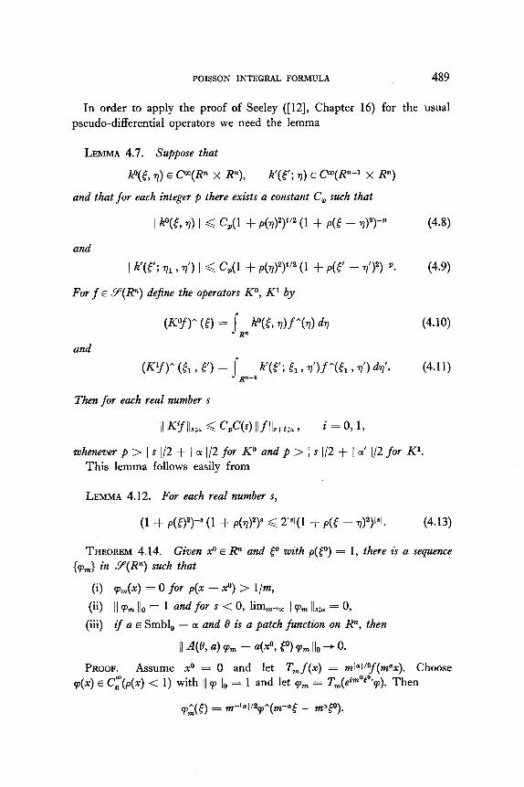
In order to apply the proof of Seeley ([12], Chapter 16) for the usual pseudo-differential &era&s we need the -lemma
LEMMA 4.7. Suppose that
h”(5, 7) E C”O(R” x R”), h’(f’; 7) E CW(Rn-l x R”)
and that for each integer p there exists a constant CD such that
I hO(& 7) I < G(l + P(7W2 (1 + PC5 - 7)“)~”
and
I w; 71 9 7') I < w + dd2Y2 (1 + P(C - 11'W.
For f E Y(Rn) define the operators K”, K1 by
F’f)A (0 = JR. h”(5, df %) 4
and
V?W (41, 5’) = /,_, W’; 51, $)f 75, 34) 4’.
Then for each real number s
II W/L;, G W(s) Ilf Ils+t:ar 9 i=O, 1,
(4.8)
(4.9)
(4.10)
(4.11)
whenewer p > I s l/2 + / 01 l/2 for K” and p > 1 s l/2 + j 0~’ l/2 for K1. This lemma follows easily from
LEMMA 4.12. For each real number s,
(1 -I p(E>2)-S (1 + P(7J2)8 < 2’8’u + /xi! - 7)2Ys’. (4.13)
THEOREM 4.14. Giwen x0 E R” and to with p(p) = 1, there is a sequence 1~~) in Y(R”) such that
(i) am = 0 for p(x - x”) > l/m,
(ii) II vm II0 = 1 and for s < 0, limm+ II vm Ils:u = 0, (iii) if a E Smbl, - OL and 0 is a patch function on R”, then
II 44 4 vm - 4x0, P) ‘pm II0 + 0. PROOF. Assume x0 = 0 and let T, f (x) = mlal/2f(max). Choose
v(x) E C,“(p(x) < 1) with 11 v Ijo = 1 and let qua = T,(eimu~“~). Then
fp;(() = m-lar112fph(m-a[ - mato).

490 LEWIS
Then (i) is clear and for s < 0
by Lebesque dominated convergence. Since T, and multiplication by eimaEO.x are isometries on Ho it suffices to show that
e-imap - T;QW, 4 vm = #m -+ 40, to) v
in Ho. Now
which tends pointwise to
(217)-” s e%z(O, 5”) qua df = ~(0, 8”) F(X).
Since X@&(X) is boonded (Cf. Seeley [12], p. 250) the convergence is in Ho.
COROLLARY 4.15. If a, E Smbl, - 01 is not identically zero and 0 is a patch function on P, then A(B, a,) does not belong to Op, - a for any s < r.
DEFINITION 4.16. Denote by ,Z - 01 the complex vector space of all formal sums u = ZkCksZuk where ak E Smbl, - a! and uk = 0 for K sufficiently large; filter ,Z - OL by the subspaces Z,. - cy. consisting of all such u with uk = 0 for K > r.
We remark here that if uk E Smbl, - 01 then
D,r D,%,(x, E) E Smblk+., - a.
Hence if 0 = &z, E ZT - 01 then
u * = ZleZ&-6..=l D,‘(iD,)’ uz//3! (4.17)
is in Z,. - 01. Here ,!I! = /?r! **a j&s,! If (T = Zua, E Z,. - 01 and U’ = Zb, E Z3 - (II then
is in Zr:,,, - 0~.

POISSON INTEGRAL FORMULA 491
THEOREM 4.19. With respect to the operations of * defined by (4.17) and product defined 4y (4.8), z - OL is aJiltered *-algebra.
We are now ready to define the quasi-homogeneous pseudo-differential (or Calderon-Zygmund) operators.
DEFINITION 4.20. A linear map A : Y -+ Y will be called a quasi- homogeneous pseudo-differential operator of order r if there exists 0 = Leak E ,JY,. - 01 such that for each integer j < Y and patch function 0 on p,
A - gsiA(e, ak) E Opiml - 0~. (4.21)
The collection of such A will be denoted by CZ, - (II and we define
cz-,=y cz,-ci. ?TZ
Define the symbol of A by o(A) = u. If A E CZ - 01, a(A) is well defined by Corollary 4.15. The main properties
of CZ - 01 are given by
THEOREM 4.22. The collection CZ - OL is closed under sums, products and A -+ At and hence is a *-algebra. The CZ, - (Y are subspaces of CZ - 01 and give CZ - OL the structure of a filtered *-algebra. Moreover the mapping a : CZ - 01+ I: - 01 is a *-homomorphism and a(A) E Z; - CL ;f and only if A E CZ,. - (Y. Finally the sequence
is exact.
(4.23)
PROOF. We here sketch the proof of the product formula. Assume that A = A(0, , ar), B = A(&, b,) where 8, = 1 on supp es. Let
a7 = a0 + a’ + ao0, ci, = are1 , hs = b,e, ,
and similarly for ci”, 6O, etc. Then
V&f Y (71,4 = (2n)Fn j- d”(7 - 8, 6) (Bf)^ (67 d5 R”
+ (2w-n j J(T’ - f’; 71, 5) (Bf )^ (71, T) d5’ p-1

492 LEWIS
= WY j j Ii077 - 6, 6) h"(5 - 7, q)f^(y) 4 d5
+ w7Y j,, j,ael ciO(T - 5, 5)
x 6'(5' - 7'; E1,7')fA(& , 7') 4 dt-
+ W-” j 4'37 - 576) ~YW(5) df
+ c=Y” j,.-,s, qT’ - 5’; 71 , 5’) x 60’% - 71, 5’ - 7’; 71, 7’)fA(7) d7 d5’
+ (217)2-2n j,,, j,,-, dt--(Tt - 5’; 71 , 6’) x P-g - 7’; 71 3 7’)f^(Tl, 7’) 4 d5
+ (2n)1-n j ci’“(T’ - [‘; T1 , 5’) bm(Tl , f’)f^(Tl , 6’) d5’ Jy-1
In the first term let
P(T - [, [) = Z,,,&iD,)B cioA(7 - [, 7) (6 - 7)6/p! + remainder terms
and note that
(t - 7y Boy! - 7,7) = (&6~o>A (5 - 777)
and obtain bounds of the form (4.8) in Lemma 4.7 to obtain estimates on the remainder. In the second term let
(i’^(T - 6, [) = ~18TlGN(i&‘)8’ doA(7 - 6; (1 , 7’) (7’ - [‘)“‘/fi!
and use (4.8) to treat the remainder to obtain a psuedo-differential operator T, with
4-2) = &=cs,. . . ,sJWJ8 a0 &c8b’/P*
The third term is a pseudo-differential operator T3 with u(Ta) = aoF. In the fourth term expand d’“(T’ - 6’; T1 , 5’) in a Taylor series about (71 , 7’) in the last variables; use (4.9) to estimate the remainders and obtain an
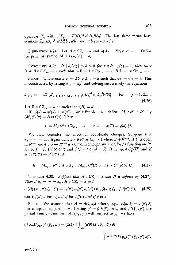
POISSON INTEGRAL FORMULA 493
operator T4 with u(T4) = E(iD,)fl a’ Dzabo//3! The last three terms have symbols za(iD*,)a’ a’D;‘b’, a’bm and amb respectively.
DEFINITION 4.24. Let A E CZ,. - LY. and o(A) = .Ez, E Z; - 01. Define the principal symbol of A as uT(A) = a, .
COROLLARY 4.25. If 1 a,(A) 1 > 6 > 0 for x E R”, p(f) = 1, then there is a B E CZ-, - 01 such that AB - 1 E Op-, - 01, BA - 1 E Op-, - 01.
PROOF. There exists u’ = .& E z-, - 01 such that uu’ = u’u = 1. This is constructed by letting b-r = a;’ and solving successively the equations
b-,-j == - url{Z;c+l-a.e=-j,l~-~-~+l(iD~)e uk @b#} for j=1,2 ,... f
(4.26)
Let B E CZ-, - (Y be such that u(B) = u’. If 1+5(x) = z,P(x) + #‘(x’) + #* E Smbl, - OT, define M,,, : Y---f Y by
CM+ f ) (4 = +W f(x). Then
T=MtiDB~CZB.,-~ and u(T) = 4(x) P.
We now consider the effect of coordinate changes. Suppose that
012 = *-* = % . Again denote x E Rn as (x1 , x’) where x’ E Rn-l. If U is open in Rn-l and $ : U -+ Rn-l is a Cm diffeomorphism, then for f a function on R” let #*f=fo(id x $-l) and $*f=fo(id x #). If ~1,~2EC~(U) and if A : Y(R”) -+ Y(R”) let
B=Mqlo#*oAo+,oM,z:C,“(R x U)+C*(R x U). (4.27)
THEOREM 4.28. Suppose that A E CZ, - (Y and B is defined by (4.27). Then~f~2=~~~=ol,,B~CZ,-~und
4B) (Xl , x’; 51 , 6’) = yl(x’) &‘> u,(A) (~1, VW); 5, , J-W 0, (4.2%
where J(x’) is the udjoint of the differential of # at x.
PROOF. We assume that A = A(0, a,) where, e.g., a,(x, 5) = a’(x’; 5) has compact support in x’. Letting y’ = I,!-l(y’), etc., and f ‘(fl , y’) the partial Fourier transform off (yr , y’) with respect to yr , we have
(ALMvzf )’ (51, x’) = (217)~” 1 (~‘0) (F’; 51,5’) d5’ Rn
x s
eiQ-~).~‘(~2f )’ (5, , y’) dy’.
409/26/3-3
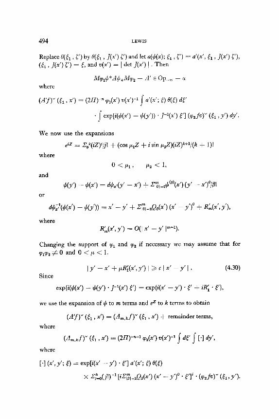
494 LEWIS
Replace e(Er , 5’) by O(S1 , 1(x’> 5’) and let a(#(~); tr , 5’) = a’(~‘, t1 , 1(x’) 0, (,$r , 1(x’) 5’) = E, and v(x’) = / det 1(x’) ) . Then
M~,#*A#,M~, - A’ E Op-, - 01 where
(Alf)’ (5, , 4 = (2W” cpl(x’) +‘)-’ j 4x’; 5) e(t) d5’
. i exp[i(W) - QWN * J-W) 5’1 (RJW (51 y Y’) 4’.
We now use the expansions
69 = Zok(iZ>j/j! + (cos plZ + i sin ~aZ)(iZ)k+l/(k + l)!
where
0 <Pll IL2 -=c 1,
and
or
#(y’) - 9(x’) = d&(y - x’) + Z;,zz2@‘(x’) (y’ - x’>‘/B!
d+&6(x’) - $(y’)) = x’ - y’ + I;,& (x’ - Y’)’ + %4x’, Y’),
where Rk(x’, y’) = O(l x’ - y' p+y.
Changing the support of q~r and q2 if necessary we may assume that for q~r9~~#0 and 0 <CL < 1.
Since 1 y’ - x’ + pR$x’, y’) I >, c 1 x’ - y’ 1 . (4.30)
exp{i(+(x’) - #(y’) . ]-1(~‘) t’} = exp{i(x’ - y’) * 5’ + iRi . E’),
we use the expansion of 4 to m terms and ez to k terms to obtain
where
(A’f)’ ([r , x’) = (A,,&)” ([r , x’) + remainder terms,
(&.lef)” CL, 4 = (2W’+1 A4 4W j d5’ j C-1 W, where
[.I (x’, y’; 69 = edi@ - y’) * 67 a’(~‘; E) 45)
POISSON INTEGRAL FORMULA 495
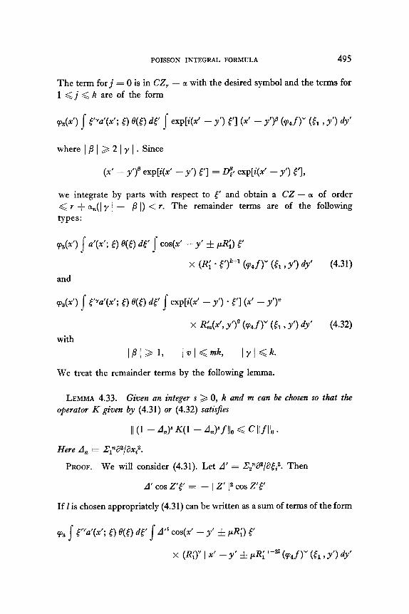
The term forj = 0 is in CZ, - 01 with the desired symbol and the terms for 1 < j :< k are of the form
FJ&‘) 1 Pa’(x’; 4) e(t7 K s exp W’ - y’) PI (x’ - Y’Y hf)” (& , y’) 4’
where I/3 1 > 2 1 y 1 . Since
(x’ - y/)8 exp[i(x’ - y’) 5’1 = D$ exp[+ - Y’) f’l,
we integrate by parts with respect to 4’ and obtain a CZ - (11 of order
G r + %(I Y I - I B I) < r. The remainder terms are of the following types:
&x') f a'(~'; t) e(t) de' j cos(x' - Y’ f PR;) 5
x (R; - t’Jk+l hf)” (51, ~3 dy’ and
(4.31)
(p2(x’) 1 (+a’(~‘; t) e(t) d5’ 1 exp[i(x’ - y’) * E’] (x’ - y’)”
x Kn(x’, Y’>’ hf)” (&> Y’> 4’ (4.32)
with
IBI 2 1, 101 <mk, IYI Gk*
We treat the remainder terms by the following lemma.
LEMMA 4.33. Given an integer s > 0, k and m can be chosen so that the operator K giwen by (4.31) OY (4.32) sutis$es
II (1 - A,)” KU - 4)sfllo < Cllfllo *
Here A, = Zl%Y/ax~.
PROOF. We will consider (4.31). Let A’ = Z2’@/8ti2. Then
A’ cos Z’f’ = - I Z’ I2 cos Z’.f
If I is chosen appropriately (4.31) can be written as a sum of terms of the form
v2 j- ya’(x’; 6) e(f) de’ $ A” cos(x’ - y’ f &) 5
x (R;)’ I x’ - y’ f PR; I-” hf>’ (51, Y’) dy’

496 LEWIS
with 1 y 1 = k + 1. Integrating by parts with respect to 6’ yields
vJ3 j d’z[(‘yu’(x’; 5) e(E)] d5’ j cos(x’ - y’ + pR;) E’
x R;’ / x’ - y’ f pR; i-” (y4f)” (E, , y’) dy’.
Now O’c[.] is a sum of terms quasi-homogeneous of degree < Y + (k + 1 - 21) 01, = v for large p(f) and thus is integrable (d[) if 2, < - / a: / . The derivatives of order j < 4s in x’, y’ of Ry / x’ - y' + pR; l--21 are O(] x’ - y’ jsk+2-2z--i) and thus to consider
(1 - OJs K(1 - 0,)s we take
2k + 2 - 21- 4s > 0. (4.34)
Terms containing ttS, j 5’ ]4S also appear. Then
[(l - 4)s q1 - 4yfl’ (& 7 x’)
is a sum of terms such as
(Cf)' (4, , x') = ~3 j Q'; 5) fX0 de'
where
X s co+’ - y’ -+ PR;) 5’1 R-(v,f)’ (E, 3 Y') W
R- = O(l +J _ y’ 12k+k-22-4s) and I Q'; E) I d C I P&'> I (1 + P(P)")",
v = Y + 1 + ol,(k + 1 - 21-t 8s) < - 101 I . (4.35)
Hence choose k and 2 so that (4.34) and (4.35) hold. To show that C is a bounded operator onL2, we use Parseval’s relation in the form IIf’ I],, = i]f/l,, . Repeated use of Minkowski’s inequality yields
(j I (CT (El , 4 I2 dx’)l” < j j d5' 4' (j I Wd)' I2 dx')"' and
(j j I (Cf)’ (El 7x3 I2 dx’ dt’)1’2
< j j dt’ dy’ (j 45 j I @W)’ I2 d~‘)“~
< j &?' (j j j I &~f)' I2 At, dy' dx'j"'
< lifll,, j dt' (j s;p I 'W'; 5) I2 dr')1'2 G Cllfllo -

POISSON INTEGRAL FORMULA 497
Let p == l/max ~ll~ . Then the lemma yields that A’ - A,,, is a bounded operator from Hzps into Ht”. The assertion that A’ is a pseudo-differential operator now follows.
The preceding theorem on the preservation of the algebra of operators under certain coordinate transformations suggests that we define pseudo- differential operators on a product of manifolds M = ki’i x M, x ... x MM . We shall give the details of this definition when 01 = (ai ,..., an), 01s = *** = an and M = R x Mz# where Mz, is a compact (n - I)-manifold without boundary. Let T(M,,) be the cotangent bundle on Mz, and
T*(M) = RR2 x T(M,,) -{O}
be the cotangent bundle on M with the zero cross-section removed. If I’ C M,, and X : V+ Rn-l is a coordinate function, let
X*f =f 0 (id x X-l) and x*f =f 0 (id x X).
A distribution f on M is in H,*(M) if and only if for each coordinate function X on V C M,, , v(d) E C:(Y). Th e d t b t is ri u ion on R” given by # -+ f (cp(X*#)) is in H,“(e); i.e. / f(y(X*#)) 1 < C 11 # Il--s;a for # E Y(Rn). Choosing a partition of unity { Vj , pj} on M,, allows a natural norm on H,“(M), denoted by Ij * Jlaio: . The spaces @(R+ x M,,) and fis([O, T) x MS,) may be defined as in (3.1) and (3.5).
DEFINITION 4.36. A linear map A on Cm(M) is in CZ - a(M) if and only if
(i) For every pair of C m functions I, #(x’) with disjoint supports
M,AM, E Op-, - a(M) (4.37) and
(ii) For every pair of Cm functions I, I&X’) with support in a coordinate neighborhood of ME, with coordinates X, the map
X,M,AMbX* E CZ - a. (4.38)
If the order of all such X,MmAM*X* is < r then the order of A is < Y and a,(A), the symbol of A, is the complex function on T*(M) defined by: if
<,, = Z;&yj dX&x’) E T(M,,) and (x1 , T) E T(R) = R2,
dx’> IcrW u,(A) (31 ,T, L,) = 4X,M,AMJ*) (~1 9 X(0 ‘~9 Y), (4.39)
where y = (ys ,..., yJ. Theorem 4.28 shows that a,(A) is well defined.
The operator A is called quasi-elliptic (of order r) at (xi, x’) EM if o,(A) f 0 on the fiber in T*(M) over (x1 , x’). Since u,(A) can be written

498 LEWIS
uniquely as or0 + 0: where ai does not depend on x1 and u,.O(xl , T, I,,) -+ 0 as 1 x1 1 -+ co, we shall call A uniformly quasi-elliptic on M if A is quasi- elliptic at each point and 0:(x1 , 7, [,,) f 0.
LEMMA 4.39. Let A E CZ, - a(M) be uniformly quasi-elliptic. Then there is a B E CZ-, - cu(M) such that
(i) BA - 1 and AB - 1 E Op-, - a(M).
(ii) If V C M,, has coordinates X, v, 4 E Cz( V) with v and z/ = 1 on an open set UC V, then for x’ E U
u(Xd%BM,X*) (~1, X(x’); 7, Y) = 4&4x, , X(x’); 7, y)
where the bj are given by (4.26) with o(X,M,AM,X*) = Z;EGTak. Lemma 4.39 now gives transparent proofs of regularity and a priori
estimates. In the following assume that A E CZ, - cx(M) is uniformly quasi- elliptic.
COROLLARY 4.40. If Au E H,“(M) then u E Hi’+‘(M) and for any real k
II u II s+r:a G C(s, 4 (II Au //s:a + II u ll.d-
COROLLARY 4.41. Let p, I/ E C,“(M) and v = 1 on a ntighborhood of support 4. If ~Au E H,*(M) then #u E Hi+‘(M) and for any real k
PROOF.
II lclu II s+r:cr < C(s, k, A P) (II FAU IL + II u Ild
#u = #B(p + 1 - P) Au + Op-m(u) = +B& + OP-w,(u).
COROLLARY 4.42. If Au E Cm(M) then u E P(M).
5. STATEMENT OF THE MAIN THEOREMS
We are ready to describe the parabolic differential operators. Let a+ be a bounded domain in P with %2+ a Cm (n - I)-manifold, 52- = complement of closure Q+ and let G% = [0, T) x Q*, and denote points in Rnfl as (t, x) where x E R”. Define the lateral boundary of G+ as X = [0, T) x Xl+. We shall consider the differential operator
A = c as(t, x) D,@ - 4 IBI<m
(5.1)

POISSON INTEGRAL FORMULA 499
where it is assumed that
(i) ua(t, x) E Cm (closure G+)
(ii) A is parabolic; i.e., there exists a constant 6 > 0 such that
Re 1 4~ 4 tB d - 6 I E P, 6 = (h ,..., L,,) E R”. (5.2) /Bl=?TZ
We assume that the coefficient of A have been extended to all of P+l, and are constant for 1 t 1 + 1 x 1 1 ar g e so that (5.2) holds for (t, x) E R”+l. Then if OL = ((or ,..., 01,+r) with cyl = m, 01~ = a*+ = cl,,, = 1, then consider A E CZ, - (Y with
a,(A) = c uB(t, x) !$B - in, (5.3) ll3l=nZ
and A is uniformly quasi-elliptic. Let @(G+) = (U : There is a 1 E @(S,) with 6 = u on G+} be equipped
with the norm
11 u (I8 = inf{/l u’ jJszT : z? = u on G+}.
We let Q be a neighborhood of EQ+ which is represented as %?+ x (- 1, 1); we suppose a normal coordinate y has been chosen so that near aQ+ points of 52 are denoted by (x’, y) wher x’ E aQ+ and - 1 < y < 1. Here y > 0 in Qf, y < 0 in 52- and y = 0 only on a.Q+. Let G = [0, T) x Q.
DEFINITION 5.4. For ( E 1 < 1 define the map of a function into its Cauchy data of order < m on the surface y = E by
R,f(t, x’) =f(t, x’, 6) @ Q,f(t, x’, c) @ a** @ II,“-‘f(t, x’, c).
where
We may define &(X) as in (3.5), and
m-1 B(X) = @ Ei"--(x).
0
The trace Lemma 3.13 yields that for s > m - Q , the map
R, : f?“(G) -+ lb(X)
is continuous.
(5.5)
500 LEWIS
Denote by @A, s) the space of distributions u E &(G+) such that Au -=- 0 in G+. Note that for x E fin+, ~(0, x) = 0 in the classical sense since u E P(G-). Let &(A, s) be the closure in B”(X) of the space of functions
{R,u : u E P(c1 G-t-), ~(0, x) = 0, Au = 0 in G+}.
Our main results are the following which were shown for some elliptic dif- ferential operators by Seeley [14].
THEOREM 5.6. There is a continuous map P, called the Poisson integral, P : &(X) -+ &A, s). For each f, Pf E Cm(G+) and lim<,,,+ R,Pf = P+f exists in the norm of lb(X). P+ is a projection of&X) onto H(A, s).
THEOREM 5.7 (Uniqueness, representation and approximation). Let u E &(A, s). Then lim,,,+ R,u = f exists in lb(X) and @A, s) is the space of such limits. iVloreover u = Pf.
The hypotheses on the coefficients of A are sufficient for the existence of a fundamental solution I’ of A (See Friedman [7]) and hence for f E CF(Rn+l) with f = 0 for t < a, we have the unique solution
u(t, x) = (A-lf) (t, x) = j: j,. r(t, x; s, z) f (s, z) dx ds
of Au = f with u = 0 for t < a. Since A is uniformly quasi-elliptic there is a B E CZ-, - (Y such that AB - 1 E Op-, - 0~. Thus iff (t, x) = 0 for t < 0, q+,(t), cpl(t) E C:(R) with v1 = 1 on [0, T] and y,,yl = I then
w-‘f = v#%of = wBf + OP-m( f ).
In the following we will use the expansion of B as a CZ - OL to obtain bounds on vlB on the spaces H,S(R”+l) and then apply Lemma 3.10 to use these bounds for operators involving A-l acting on spaces fis(Sr).
6. CONSTRUCTION OF P, P+, AND THE BASIC LEMMAS
We suppose that a Cm volume element da has been chosen on aQ+ so that for functions f supported near X
j j,,f (t, x’, Y) = j j, j’,f (6 x’9 Y) dY dt da*

POISSON INTEGRAL FORMULA 501
We define the differential operator A* which is the adjoint of A by
s (Au) v* = s
u(A*v)* sT ST
for u, v E C:(P+l) with ~(0, x) = v(T, x) = 0. Near X, A has the form
A = f A,(y) Or-’ - ; (6.1) 0
where for each y, Aj(y) is a spatial differential operator of order <i on X. For 1 E 1 < 1 let G, = G n {y > E}. Then for smooth u and v with
u(0, x) = v(T, 2) = 0, (6.2)
Green’s formula becomes
j, u(A*v)* = j, Auv* + j (UY, Rev) X
where (f, g) = 2YF-lfjgj* and G& is a matrix of the form
i
m-1 I(E) Am-, A4 *-* Aok) ~m~,*l(6, * * :
ac=-i i’ Aoh) 0
Ad4 AOH 0 *** 0
A,(c) 0 . . . 0 1
where Aj,k(~) = Aj(e) + t erms of order <i. Note that a/at does not enter into Green’s formula by the initial conditions (6.2). Since A is parabolic A,(E) is a nonvanishing function and thus GYE is invertible, its inverse being a matrix of differential operators.
For f = (f. ,.,.,f& an m-tuple of distributions on R x E&r+ with fi(t, x’) = 0 for t < 0, define RTf by
<R:f, v)s, = <f, Rv)x
for y E Cz(Sr); i.e., if the fi’s are locally integrable functions
<R:f, v’)s, = j, (f, &P) = mfl s fi(Dth)* j&o x
m-1
= ,T;, (fi @ d;;(Y - ‘), y)sT.

502
Hence
LEWIS
K+f = c fi 0 %,(Y - ~1. j=O
(6.3)
We are now ready to define P. For f E E%(X) let
Pf = A-l(R,$Yof). (6.4)
Since the map 4 + $ @ 8::!(y) is continuous from &X) into &s-i-1/2(Sr) for s < 0, we have that if f E l&X), s < t, then R,*6Yo f E &-“(S,) and Pf E I+(&). Ifs = 0, Pf is an L2 function. The essential step in the proof of Theorem 5.6 is now given by the following lemma, which for elliptic equa- tions is due to Seeley ([14], p. 794). Let
Rl.Ef (t, x’) =f (t, x’, 6) and B = (0, T] x as;)+.
LEMMA 6.5. Let g E C:(2). Then for each j and k
L&g = R,,, D,‘A-l D,‘Rcog
converges uniformly on X to a limit L&g as E -+ Of. Lii is a CZ - 01’ of orda < (j + h) - (m - 1) on R x &?+ and
u,+~-,+~(L&) (t; T, Z,,) = (2l7)-1 j, ni’“{~oo”ol(A1(0)) (t; Z,,) n”-’ - iT}-‘dn
(6.7)
where I’ is a path surrounding the roots of Eul(AE(0)) ram-l - ir which lie in (Im n > O}.
PROOF. Let B E CZ-, - 01 be such that BA - 1 E Op-, - 01. It suffices to consider MWIA-lMQzR1*,og where v1 , pls E Cz(R x Q), and we suppose coordinates X = (t, X, ,...; X, , y) h ave been chosen so that y is one of the coordinates. Then if v = 1 on suppfl y1 / + 1 ~a I), C = XJR~lA-lMVZX*, and
o(X,M,AM,X*) (X(t, x’, y); 7, [‘, y) = JYE,a(A,(y)) n”+’ - ir
on supp(X,(I vr 1 + / ~a I)) where of course a(A,(y)) does not depend on 7 or n; we have by Lemma 4.39 that u(C) = (X,~z’,~-,b,) u(X,& and the b, are given by (4.26). Let

POISSON INTEGRAL FORMULA 503
and suppose that O(T, c, n) = 1 for p(~, c, n) > 1. Then
Ds(M&‘M,, - &>--NCJ Dyj
is of order <j-N-i-or.8 and for -N<--*j3-j+1(~1/2+$, DB(MalA-lMa - Zr,-&‘r) D,k is a continuous function on R x D for u E L2 by tie Sobolev Lemma 2.9. Hence we must consider only
Following a method of Seeley ([14], p. 796), we approximate R&g from “outside” Gf. Let ‘Y(S) E Cz(- 1, - l/2) be such that s a(s) ds = 1. Let a,(s) = ~‘Y(P). Then as distributions,
ILj+‘(Dja) (ps) g(t, x’) 4 DyjR;og
as f.L--+oo. If f = X,psg, ‘pr* = X,cp, and 2’ = X(x’) = (Xs ,..., X,), then for y > 0
(X,C, DyjR&g) (t, Z’, y) = (2l7)+ q* j& /R./” f+, f’, n) nW(p-‘n) -cc
x b,eir” dnf h exp[iZ’t’ + &] df dr. (6.9)
Formula (4.26) yields that b, = {Zomml(Al(y)) P--~ - k}z+na-l x (function holomorphic in (7, e’, n) and bounded by a polynomial). For p(T, c) = 1 and (t, x’, Y) near X, ~omG4(~)) nrn-l - iT is a polynomial of degree m in n whose zeros in (Im n > 0} lie in a compact set K C (1 n 1 < R}, which does not intersect the real axis; the zeros for p(T, t) = p lie in PK. Let r(p) = boundary of (1 n 1 < max( 1, Rp)] n {Im n > 0} and assume e(T, t’, n) = 1 for p(T, 5’, n) > 1, where ti is now allowed to be complex. Since aA decays exponentially for Im n >, 0 we may replace szW **a in (6.9) by Ji-(p(T,C~)) -*a and take (limu+oo ) under the integral sign to obtain that
(6.9) = (2W-l VI* I,, [I Obtnjeif’n dn f” exp[iZ’r + itT] df’ dr. rb(T,C’)) 1
This function is Ca, for y > 0 and
lim R,,, D,‘“C, D,jR&g(t, 2’) c-+0+
[(2Ly s Ob#+k dn f h exp[iz’f + itT] df dT Rfi r(P(T,P’))
1
504 LEWIS
+ terms with powers of n of degree < j + k. Note that the term in [.I is quasi-homogeneous of degree 1 ij + K + 1 for p(~, ,$‘) > 1. This is then a
CZC,i,k,l - a’(R x aQ+) and taking 2 = - m shows the principal symbol of Lij is given by (6.7).
LEMMA 6.10. Let g E C:(X). Then
II -Gig I/s;x e C(s, kj) II g /ls+j+k--m+1;x * PROOF. It suffices to consider the terms which arise from the operators
C,; i.e., the operators
where
&g(t; z’) = j,, CljlcfA exp[iZ[’ + it71 d[’ &
Cljk(4 2’9 r; 7, 5’)
= (2II)-l D,” jT(p(I,I,jj 0(~, [‘, n) nifkb,(t, Z’, r; T, E’, n) eiGn dn.
But if Ci, denotes the Fourier transform of Crj, with respect to (t, z’) we
can easily show that
(qj,f)^ (s, $) = I,, Cl”jk(s - 7,~’ - 5’3 E; 7, f’)f’-(~, 8) dT d5’
and that for any integer p
1 c&(S - 7; 7’ - t’, E; 7, 5’) 1
< c,(l + p(S - 7, 7’ - t’)2)-p . (1 + PC’-, t’)2)t’2
with t = j + k - I + 1 and apply Lemma 4.7.
COROLLARY 6.11. If g E &+j+k--m+l(X), then Lij f + L$ f in e(X) as EdOf.
LEMMA 6.12. For s < 3 there is a constant C = C(s) such that
II ~-‘m&f Ils;T < c Ilf: &x> II * (6.13)
For s > 0 there is a corresponding bound in the norm of f@(G+) of Pf = A-lR;CYOf lo+.

POISSON INTEGRAL FORMULA 505
PROOF. The case s < Q was done following (6.4). For km a multiple of m andO:<j<m-1 let
gj = hl+ R,,, D;A-‘R& f,
and for m < j < mk - 1, solve successively for gi as the solution for D,jw in the equations
Then
DYi-” (Z,,mA, D;-‘W - (t) W) = Dj,-“(Aw) = 0.
II gj llrnk-~-1,2:X d c Ilf: B”“W II *
By the extension Lemma 3.19 there is a z, E fikm(ST) with
&cm--1s = (gd and II4 km;T < cz 11 gj hnk-j--1/2:X < c Iif: Bk”(X) 11 -
Let u = A-lR$Y,, f in G+ and u = v in G-. Then u E L2(ST) and for
= lim i
Amp” + lim lYl>E s
x (R,u, Ql$Rgp)
- lim s x (R-,u, Ol$R-,cp)
= lim I
Amp*. V<O
Since Av E &km-m(Sr) and its Cauchy data on X of order < km - m is zero, Au E fikm-“(Sr) by Corollary 3.18 and u E fikm(ST) and
II 24 II km:T < c ilf: Bkm(x) iI *
To show (6.13) for s 3 0 let Ext : Akm(G+) -+ Bk”(ST) be constructed as in Corollary 3.18. Then the map f + Ext(Pf) is continuous for s = 0 and s = km and by Corollary 2.7 on interpolation it is also continuous for 0 < s .< mk.
We show that Pf is a projection. If f E f%(X) define
(6.14)
LEMMA 6.15. P+ + P- = 1.

506 LEWIS
PROOF. Let f E Cz(X)m and 97 E C~(Sr) have support near X. Then
= (Pf,A*ph =iis j,g,>8(PfHA*d*
= lim j x
(@&Pf, l&p) - lim jx@-&Zf, R-e)
= /W'+f+ P-f), %v). s
Since QZs is invertible and R,p arbitrary, the lemma is shown.
DEFINITION 6.16. Let H* = {R,u : u E f@(S,), Au = 0 in G*}.
LEMMA 6.17. The space l@(X) is the direct sum of H+ and H- and P+ are the corresponding projections.
PROOF. Since f = P+f + P-f it suffices to show that
(i) range (P*) C Hk and
(ii) H+ n H- = 0.
If f = P+g and u = A-lR$Z,,g E fim(G+), then Au = 0 in G+ and R,u = P+g = f. If Au* = 0 in G* and R,u+ = R,,u- then define w = uf in G+ and w = u- in G-. Then w E fim(Sr) and Aw = 0 in ST . Hence w = 0 and R,u+ = R,u- = R,w = 0.
PROOF OF THEOREM 5.6. The continuity of the map P defined by (6.4) is shown by Lemma 6.12. The existence of lim,,,+ RJ’f is given by Corollary 6.11.
It remains to identify P+(&(X)) as &(A, s). If u E C:((O, T] x Rn) and Au = 0 in Gf then R,u E H+ and R,,u E ptRou. If uj E C:((O, T] x Rn), Auj = 0 in G+ and R,u, -+ f in &s(X), then f = lim R,u* = lim P+R,uj = P+f and &(A, s) C P+(&(X)). C onversely, if P+f =.f let ( fj} C Cp(&m be such that fi ---f f in As(X). Let uj = Pfi . Then ui E Cm (closure G+), Au, = 0 in Gf and R,uj = P+fj + P+f = f. Thus P+(&(X)) C &(A, s).
7. PROOF OF THEOREM 5.7
We begin with a uniqueness result.

POISSON INTEGRAL FORMULA 507
LEMMA 7.1. If u E @A, s) and there exists lim,,,+ R,u = f in &s(X), thenu=PfandfE&(A,s).
PROOF. Ifs = m then f = R,u E H+ and f = P+f. Let v = Pf - u in Gf. Then lim,,,+ R,v = 0 and by Corollary 3.16 the function w = v in Gf, w = 0 in G- is in E?4in(Sr). If v E C~(Sr) then
/ w(A*q~)* = I,ms J,V,,6w(A*~)* = - lim 1 (O&Rsv, R,q) = 0 f+ x
and Aw = 0; hence w = 0. Let now s be arbitrary and u E &(A, s). Let (t, x) E G,, = {y > 2~ > 01.
Since u is Cm in Gf we have u = A-1R,*@8R,u in G, for 0 < 8 < E. Let q~, # E P(G), & = 0, y(t, x) = 1 in G,, and # = 1 in {I y / < c}. Then u(t, x) = (M,A-lM,R,&R,u) (t, x) and M,A-lM, E Op-, - 01. Since R$&R,u -+ R,*GZ?,,f in @-“(Sr) for t < min(s, 4) and the map v -+ v(t, x) is continuous on fir(G) for I > (n + m)/2 = ) 01 l/2, we have
u(t, x) = (M,A-‘M+R&R,u) (t, x) -+ (M,A-lM,R,*LTOf) (t, x)
= (Pf) (4 x)
and
P+f = lim R,Pf = lim R,u =f
The proof of Theorem 5.7 will be completed if we show that lim,,s+ R,u exists in J%(X) f or u E &(A, s). This follows trivially from the trace theorem fors>m-4.
LEMMA 7.2. If u E &(A, s) then R,u converges in l%(X) as E + 0+ and
11 !%+ R,u : I+(X) (1 < C II u : fi8(G+) II .
PROOF. LetBbetheCZ-,--sothatAB-l,AB-IEOp-,-a. Then u = BAu + Op-,(u) and it suffices to show that if w E &s-m(G) and w = 0 in Gf, then lim,,,, R,,,(D,jBw) exists in Hi-+l12(R x EZ2+). Note that if Bw has normal derivatives of order < m on R x 8Qf we may solve for the normal derivatives of order 3 m in terms of the Cauchy data of order < m since ABw = w + OpJw).
Without introducing any new notation we assume that G = Rn+l and G+ = {xn+r = y > 0} and define the operator A, by
(A+f)^ (7, r, n) = [(l + 1 r Inz + i7)l’” - in]f^(7, r, n).

508 LEWIS
Then A+A is an isomorphism on H,S(R*l+l) for all S. The operator A, resem- bles the parabolic Bessel potential operator A in that
LEMMA 7.4. Let u E 9”(Rn+l) have support in {y .< O}. Then S$ has support in {y < 01.
When A is any operator on Y define its successive commutators with AL by
C,,(A, A+) = A, C,+l(A, A,) = C,(A, A,) A, - A+C,(A, A+).
LEMMA 7.5. If A E CZ - pi is of order < Y then C,(A, A,) has order < Y.
PROOF. We may assume that A = A(B, a,) with, e.g.,
a;(x; 7, f’, n) = aF(7, t’, n) = 0.
Now C?(~(T, .$ = 1) is a nuclear space (Yosida [15]); hence given any finite collection of seminorms (1 * IP}p=l,,..,N on Cm(p(~, E) = 1) we may write
a,(4 x; 7, 5) = zA,@k(t, 2) sk(~, 5)
with Z 1 A, / < co, {&} bounded in 9’(Rn+l), and {I SR(7, E) lP}p=l,...,~ bounded. Then A(8, a,) = ZIXkMOkSlc where S, is a translation invariant operator of order < Y and C,(A(e, a,), A,) = 2&Cj(M0,, A+) Sk; thus we are reduced to showing that Cj(M,+ , A,) is an operator of order 0, and obtaining bounds which depends only on the seminorms of {aR}. Let A be multiplication by @ and A(k) be multiplication by (a/ay)l, @. Define A, by (A, f)^ (7, F, n) = (1 + / E’ Irn + iT)llm f h (T, r, n); then A, = A, - ajay. If C,(A, An) = A and C,+l(A, A,J = C,(A, A,) A, - A,C,(A, A,), then
( 1 $ C&J”“‘, A,) - Cj(Ack), A\,) ($) = Cj(A(ICfl), A,)
and by induction on k it follows that C,(A, A,) = 2,,k~ikCj(A(li--j’, A\,), where cjk are the combinatorial coefficients. If we view Cj(A(“-j), &J as a one parameter family of operators Cj(Aik-j), A,) where A:-‘) is the operator on Y(R”) given by
(A:-“& (t, x’) = (;)“-’ @(t, x’, y) f (t, x’)
and A, is the Bessel potential operator on Rn, we see that
11 Cj(A(k-j), a,) : L2(R”+l) +L2(Rn+l) /I
< s;p 11 Cj(Af-j’, A\,) : L’(R”) -+ L’(R”) /) . (74

POISSON INTEGRAL FORMULA 509
Since A, E CZ, - 01’ and AF-j’ E CZ, - 01’, we see by applying Theorem 4.22 that Cj(A:“-j’, &J E CZ-j+l - a’(j 3 1) and the right hand side of (7.6) is finite. If - s is a negative integer, then C,(A, A+) is continuous from H;” into His if and only if d;‘Cj(A, A,) A+” is bounded onL2. An induction on s yields A;“C,(A, A+) A+S = ,Z:=, c,~A$,+~(A, A,) and a;” is of order - 1. Bounds for C,(A, A,) as an operator on H,” for s a positive integer and for all s real are obtained by taking adjoints and interpolating.
We can now complete the proof of Lemma 7.2. By induction on K we show that if w E Hws for s > - K - + there exists lim,,,+ DVzBw(*, y) in H~?“-z-1’2 with a corresponding bound in norm. We use the formula
Bw = C,(B, A,) A;“w + 2;=1~jkA:BA;‘w, (7.7)
with appropriate constants cjk . Since A;” E Op-, - (y: the first term has y derivatives of order 1 < m with boundary values in Hj?k+mm-1-1i2 by the trace Lemma 3.13. For 1 <j < K, lim,,,, DvzBA~jw(*,y) exists in H~?j+m-z-1’2 for all 1 by the inductive hypothesis; thus by the special form of A, = A, - ajay, where A, : H,‘, + H”;’ is an isomorphism for all Y, we have that lim,,,,+ D,zA+jBA;iw(., y) exiits in Hi?m-z-1’2 for all 1. This proves Lemma 7.2 and Theorem 5.7.
8. REMARKS
The proof of Lemma 7.2 on regularity at the boundary of solutions of Au = 0 did not require the operator to be invertible; only the “pseudo- inverse” B E CZ, - 01 was used; thus results on regularity at the boundary could be obtained for quasi-elliptic differential operators.
The essential step in using estimates for operators on Rn to obtain results for operators on the lateral boundary X was Lemma 3.10. The techniques might apply to operators with the uniqueness results of that lemma.
We have assumed that the lateral boundary data had “zero initial value”. This is not too restrictive, since for s < 0, Lemma 3.8 gives that f~ E@(X) if and only if f is a continuous linear functional on
fP(X)n {p : v(T, x') = O}.
If we wish to decide which lateral boundary value problems are well posed for (5.1), we have a bijection between solutions in Bs(G+) and &(A, s) given by the Poisson integral P and we are reduced to considering the action of the boundary operators on the Poisson integrals. We also have shown that solutions in &(G+) can be approximated by solutions in Cm (closure G+).
J. C. Polking [13] has considered a related problem. Let A be a parabolic
409/26/3-4

510 LEWIS
operator (i.e. am(A) f 0) on [0, T] x M, where M is a compact manifold without boundary. Define the Cauchy data of a function u to be R,,u = ~(0, .) @ u(T, .). H e constructed a projection onto
{R,u : Au = 0 in (0, T) x M)
in the appropriate Sobolev space (H”-“/“(M))“. Note that in this problem there is no lateral boundary to be considered.
Parabolic singular integrals (quasi-homogeneous pseudo-differential opera- tors of order 0) have been used for second order parabolic equations by Fabes and Jodeit [4]. Their techniques use parabolic singular integrals on the manifold X which are defined with a different kernel for a,(A) (essentially those operators which can be dominated by convolution with an L1 function on a strip. Their methods assume only the existence of a fundamental solution, and they obtain results valid for L”, 1 <p < CO, whereas we here consider only the L2 theory. Fabes and Jodeit [5] and Jodeit [9] considered equations of order higher than two; in these papers aQ+ was taken to be a hyperplane.
Boutet de Monvel [2] has developed a general theory of pseudo-Poisson kernels in the elliptic case. The Poisson integral of Seeley is an example. We have not here attempted to define pseudo-Poisson kernels in general for the quasi-homogeneous or parabolic case. Suffice it to say that our Poisson integral should be an example of such.
REFERFNCPS
1. N. ARONSZAJN AND K. T. SMITH. Theory of Bessel potentials, part I. Ann. Inst. FOUY. Gren. 11 (1961), 385-475.
2. L. BOUTET DE MONVEL. Comportement d’un operateur pseudo-differentiel sur une variete a bord. II. Pseudo-noyaux de Poisson. J. d’AnaZ. Math. 17 (1966), 255-304.
3. A. P. CALDER~N. Boundary value problems for elliptic equations. Joint Soviet- American Symposium on Partial Diff. Eqs. Nososibi~s~ (1963), 303-304.
4. E. B. FAB~ AND M. JODEIT, JR. Boundary value problems for second order parabolic equations. A.M.S. Symposia in Pure Math., Vol. X, 82-105.
5. E. B. FABES AND M. JODEIT, JR. Singular integrals and boundary-value problems for parabolic equations in a half-space. University of Minnesota School of Mathe- matics, 1967.
6. E. B. FABER AND N. M. RIVIERE. Singular integrals with mixed homogeneity. Studio Math. 27 (1966), 19-38.
7. A. FRIEDMAN. “Partial Differential Equations of Parabolic Type.” Prentice- Hall, Englewood Cliffs, New Jersey, 1964.
8. L. H&WUNDER. “Linear Partial Differential Operators.” Academic Press, New York, New York, 1963.

POISSON INTEGRAL FORMULA 511
9. M. A. JODEIT, JR. Symbols of parabolic singular integrals and some La boundary value problems. Dissertation, Rice University, 1967.
10. J. J. KOHN AND L. NIRENBERG. On the algebra of pseudo-differential operators. CPAM 18 (1965), 269-305.
11. P. KREB. Distributions quasi-homogenes. Generalisations des integrales sin- gulieres et du calcul symbolique de Calderon-Zygmund. CRAS Paris 261 (1965), 2560-2563.
12. R. S. PALAIS, ED. “Seminar on the Atiyah-Singer Index Theorem.” Princeton University Press, Princeton, N. J., 1965.
13. J. C. POLKING. Boundary value problems for parabolic systems of partial differen- tial equations. A. M. S. Symposia in Pure Math. Vol. X, 243-274.
14. R. T. SEELEY. Singular integrals and boundary-value problems. Am. J. Math. 88 (1966), 781-809.
15. K. YOSIDA. “Functional Analysis.” Academic Press, New York, 1965.