Accepted Manuscript

A Permanent MRI Magnet for Magic Angle Imaging Having its Field Parallel

to the Poles

John V.M. McGinley, Mihailo Ristic, Ian R. Young

PII: S1090-7807(16)30129-X

DOI: http://dx.doi.org/10.1016/j.jmr.2016.08.001

Reference: YJMRE 5924

To appear in: Journal of Magnetic Resonance

Received Date: 6 July 2016

Revised Date: 5 August 2016

Accepted Date: 5 August 2016

Please cite this article as: J.V.M. McGinley, M. Ristic, I.R. Young, A Permanent MRI Magnet for Magic Angle

Imaging Having its Field Parallel to the Poles, Journal of Magnetic Resonance (2016), doi: http://dx.doi.org/

10.1016/j.jmr.2016.08.001

This is a PDF file of an unedited manuscript that has been accepted for publication. As a service to our customers

we are providing this early version of the manuscript. The manuscript will undergo copyediting, typesetting, and

review of the resulting proof before it is published in its final form. Please note that during the production process

errors may be discovered which could affect the content, and all legal disclaimers that apply to the journal pertain.

1

A Permanent MRI Magnet for Magic Angle Imaging Having its

Field Parallel to the Poles

John V.M. McGinley, Mihailo Ristic1, Ian R. Young

Imperial College London, Mechanical Engineering Department

South Kensington Campus, Exhibition Road, London SW7 2AZ, United Kingdom

+44 (0) 20 7 594 7048, m.ristic@imperial.ac.uk

Corresponding author

Mihailo Ristic Imperial College London, Mechanical Engineering Department

South Kensington Campus, Exhibition Road, London SW7 2AZ, United Kingdom

+44 (0) 20 7 594 7048

m.ristic@imperial.ac.uk

Abstract—A novel design of open permanent magnet is presented, in which the magnetic field is oriented parallel to the planes of its poles. The paper describes the methods whereby such a magnet can be designed with a field homogeneity suitable for Magnetic Resonance Imaging (MRI). Its primary purpose is to take advantage of the Magic Angle effect in MRI of human extremities, particularly the knee joint, by being capable of rotating the direction of the main magnetic field B0 about two orthogonal axes around a stationary subject and achieve all possible angulations. The magnet comprises a parallel pair of identical profiled arrays of permanent magnets

backed by a flat steel yoke such that access in lateral directions is practical. The paper describes the detailed optimization procedure from a target 150 mm DSV to the achievement of a measured uniform field over a 130 mm DSV. Actual performance data of the manufactured magnet, including shimming and a sample image, is presented. The overall magnet system mounting mechanism is presented, including two orthogonal axes of rotation of the magnet about its isocentre.

Keywords— Permanent magnet, Magnetic Resonance Imaging (MRI), Magic Angle imaging, Magnet design

1 Corresponding author

2

1. Introduction

Magnetic Resonance Imaging (MRI) is the gold standard in

many areas of medical diagnostics owing to its unrivalled

ability to differentiate soft tissue structures, while 2D

sections and 3D images of the anatomy can be obtained at

arbitrary oblique angles. However, conventional MRI fails

to detect the signals from tissues in which dipolar coupling

dominates the relaxation mechanism and results in very

short transverse relaxation time , making signal

acquisition very difficult. This is typical for tissues

containing significant amounts of highly organized collagen,

such as cortical bone, tendons ligaments and cartilage, in

which their relaxation times can be changed by very large

factors (typically >10) by changing the angle θ between the

tissue and the main magnetic field. The orientation where

the angular factor for dipolar coupling (3 cos2 θ -1) vanishes

(when θ = 54.7° or, by symmetry, 125.3°) is what is termed

the Magic Angle (MA) [1]. Thus MR Imaging at this ideal

MA setting maximizes , which makes MA imaging highly

suitable for micro-structure investigations offering much

better signal-to-noise ratio and image resolution [2] . Recent

work has demonstrated how the MA effect can be used to

analyse ligaments [3], meniscus [4] and articular cartilage

[5] in terms of collagen fibre orientation, demonstrating

promising solutions for future clinical diagnostics. Such

investigation would be invaluable, for the preoperative

assessment of patients being considered for knee

replacement surgery, where in the US alone there are about

700,000 such procedures carried out annually. Another

important area of application lies in the MA imaging of the

peripheral nervous system in the body [6].

Unfortunately, in the range of magnet designs currently

available for MRI, the required relative movement between

the magnet field direction and the body is highly restricted

or just impossible. For this reason in-vivo MA studies of

ligaments and tendons reported to date have been restricted

to the Achilles tendon [2] and the elbow [7].

The types of magnets suitable for use in MRI have been

reviewed [8-10]. Essentially they fall into three main

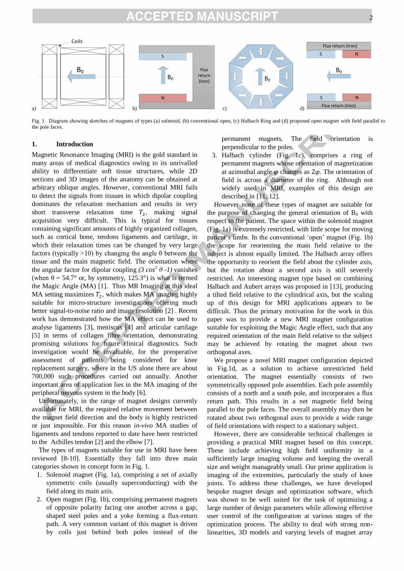
categories shown in concept form in Fig. 1.

1. Solenoid magnet (Fig. 1a), comprising a set of axially

symmetric coils (usually superconducting) with the

field along its main axis.

2. Open magnet (Fig. 1b), comprising permanent magnets

of opposite polarity facing one another across a gap,

shaped steel poles and a yoke forming a flux-return

path. A very common variant of this magnet is driven

by coils just behind both poles instead of the

permanent magnets. The field orientation is

perpendicular to the poles.

3. Halbach cylinder (Fig. 1c), comprises a ring of

permanent magnets whose orientation of magnetization

at azimuthal angle changes as . The orientation of

field is across a diameter of the ring. Although not

widely used in MRI, examples of this design are

described in [11, 12].

However none of these types of magnet are suitable for

the purpose of changing the general orientation of B0 with

respect to the patient. The space within the solenoid magnet

(Fig. 1a) is extremely restricted, with little scope for moving

patient’s limbs. In the conventional ‘open’ magnet (Fig. 1b)

the scope for reorienting the main field relative to the

subject is almost equally limited. The Halbach array offers

the opportunity to reorient the field about the cylinder axis,

but the rotation about a second axis is still severely

restricted. An interesting magnet type based on combining

Halbach and Aubert arrays was proposed in [13], producing

a tilted field relative to the cylindrical axis, but the scaling

up of this design for MRI applications appears to be

difficult. Thus the primary motivation for the work in this

paper was to provide a new MRI magnet configuration

suitable for exploiting the Magic Angle effect, such that any

required orientation of the main field relative to the subject

may be achieved by rotating the magnet about two

orthogonal axes.

We propose a novel MRI magnet configuration depicted

in Fig.1d, as a solution to achieve unrestricted field

orientation. The magnet essentially consists of two

symmetrically opposed pole assemblies. Each pole assembly

consists of a north and a south pole, and incorporates a flux

return path. This results in a net magnetic field being

parallel to the pole faces. The overall assembly may then be

rotated about two orthogonal axes to provide a wide range

of field orientations with respect to a stationary subject.

However, there are considerable technical challenges in

providing a practical MRI magnet based on this concept.

These include achieving high field uniformity in a

sufficiently large imaging volume and keeping the overall

size and weight manageably small. Our prime application is

imaging of the extremities, particularly the study of knee

joints. To address these challenges, we have developed

bespoke magnet design and optimization software, which

was shown to be well suited for the task of optimizing a

large number of design parameters while allowing effective

user control of the configuration at various stages of the

optimization process. The ability to deal with strong non-

linearities, 3D models and varying levels of magnet array

a)

B0

Coils

b)

B0

S

N

Flux return (Iron)

c)

B0

d)

S

S

N

N

Flux return (Iron)

Flux return (Iron)

B0

Fig. 1. Diagram showing sketches of magnets of types (a) solenoid, (b) conventional open, (c) Halbach Ring and (d) proposed open magnet with field parallel to the pole faces.

3

resolution, were shown to be the key for successfully

achieving the novel magnet design.

The next section describes the concept of the new magnet

in more detail. Section III presents the details of the magnet

design and optimization method, while the results are

summarized in Section IV, together with an outline of a

moveable MRI magnet system that is currently under

construction. Discussion and conclusions are presented in

Section V.

2. The Magnet concept

The new MRI magnet was primarily intended to meet the

requirements of MA imaging studies of the extremities,

particularly the knee, and also feet, elbows and hands. Being

based on permanent magnets, the target field strength was

set at 0.15 T, which is comparable to existing permanent

magnet MRI systems for musculoskeletal imaging. The

diameter spherical volume (DSV) was targeted at 150 mm

centred on the origin, or the isocentre of the magnet, with a

pole gap of 22 cm.

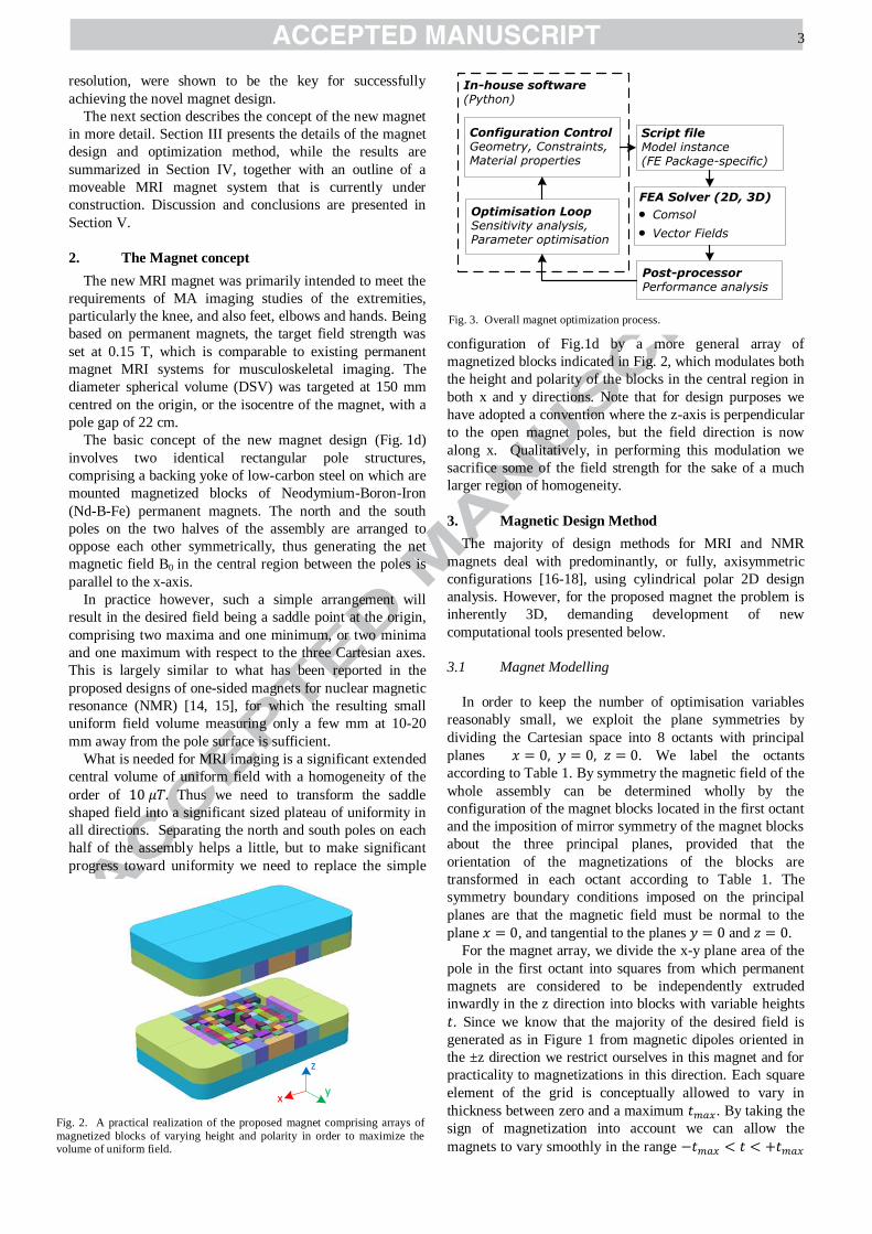
The basic concept of the new magnet design (Fig. 1d)

involves two identical rectangular pole structures,

comprising a backing yoke of low-carbon steel on which are

mounted magnetized blocks of Neodymium-Boron-Iron

(Nd-B-Fe) permanent magnets. The north and the south

poles on the two halves of the assembly are arranged to

oppose each other symmetrically, thus generating the net

magnetic field B0 in the central region between the poles is

parallel to the x-axis.

In practice however, such a simple arrangement will

result in the desired field being a saddle point at the origin,

comprising two maxima and one minimum, or two minima

and one maximum with respect to the three Cartesian axes.

This is largely similar to what has been reported in the

proposed designs of one-sided magnets for nuclear magnetic

resonance (NMR) [14, 15], for which the resulting small

uniform field volume measuring only a few mm at 10-20

mm away from the pole surface is sufficient.

What is needed for MRI imaging is a significant extended

central volume of uniform field with a homogeneity of the

order of Thus we need to transform the saddle

shaped field into a significant sized plateau of uniformity in

all directions. Separating the north and south poles on each

half of the assembly helps a little, but to make significant

progress toward uniformity we need to replace the simple

configuration of Fig.1d by a more general array of

magnetized blocks indicated in Fig. 2, which modulates both

the height and polarity of the blocks in the central region in

both x and y directions. Note that for design purposes we

have adopted a convention where the z-axis is perpendicular

to the open magnet poles, but the field direction is now

along x. Qualitatively, in performing this modulation we

sacrifice some of the field strength for the sake of a much

larger region of homogeneity.

3. Magnetic Design Method

The majority of design methods for MRI and NMR

magnets deal with predominantly, or fully, axisymmetric

configurations [16-18], using cylindrical polar 2D design

analysis. However, for the proposed magnet the problem is

inherently 3D, demanding development of new

computational tools presented below.

3.1 Magnet Modelling

In order to keep the number of optimisation variables

reasonably small, we exploit the plane symmetries by

dividing the Cartesian space into 8 octants with principal

planes . We label the octants

according to Table 1. By symmetry the magnetic field of the

whole assembly can be determined wholly by the

configuration of the magnet blocks located in the first octant

and the imposition of mirror symmetry of the magnet blocks

about the three principal planes, provided that the

orientation of the magnetizations of the blocks are

transformed in each octant according to Table 1. The

symmetry boundary conditions imposed on the principal

planes are that the magnetic field must be normal to the

plane , and tangential to the planes and .

For the magnet array, we divide the x-y plane area of the

pole in the first octant into squares from which permanent

magnets are considered to be independently extruded

inwardly in the z direction into blocks with variable heights

. Since we know that the majority of the desired field is

generated as in Figure 1 from magnetic dipoles oriented in

the ±z direction we restrict ourselves in this magnet and for

practicality to magnetizations in this direction. Each square

element of the grid is conceptually allowed to vary in

thickness between zero and a maximum . By taking the

sign of magnetization into account we can allow the

magnets to vary smoothly in the range

xy

z

Fig. 2. A practical realization of the proposed magnet comprising arrays of

magnetized blocks of varying height and polarity in order to maximize the volume of uniform field.

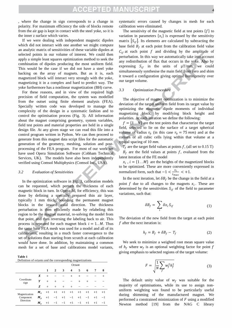
Configuration ControlGeometry, Constraints, Material properties

Optimisation LoopSensitivity analysis,Parameter optimisation

Script fileModel instance(FE Package-specific)

In-house software(Python)

FEA Solver (2D, 3D)

· Comsol

· Vector Fields

Post-processorPerformance analysis

Fig. 3. Overall magnet optimization process.

4

, where the change in sign corresponds to a change in

polarity. For maximum efficiency the side of blocks remote

from the air gap is kept in contact with the steel yoke, so it is

the inner z surface which varies.

If we were dealing with independent magnetic dipoles

which did not interact with one another we might compute

an analytic matrix of sensitivities of these variable dipoles at

selected points in our volume of interest. We could then

apply a simple least squares optimization method to seek the

combination of dipoles producing the most uniform field.

This would be the case if we did not have a steel yoke

backing on the array of magnets. But as it is, each

magnetized block will interact very strongly with the yoke,

magnetizing it in a complex and hard to predict way. The

yoke furthermore has a nonlinear magnetization (BH) curve.

For these reasons, and in view of the required high

precision of field computation, the system was modelled

from the outset using finite element analysis (FEA).

Specially written code was developed to manage the

complexity of the design in a systematic fashion and to

control the optimisation process (Fig. 3). All information

about the magnet comprising geometry, system variables,

field test points and material properties are held in a single

design file. At any given stage we can read this file into a

control program written in Python. We can then proceed to

generate from this magnet data script files for the automatic

generation of the geometry, meshing, solution and post-

processing of the FEA program. For most of our work we

have used Opera Simulation Software (Cobham Technical

Services, UK). The models have also been independently

verified using Comsol Multiphysics (Comsol Inc., USA).

3.2 Evaluation of Sensitivities

In the optimization software in Fig. 3, calibration models

can be requested, which perturb the thickness of each

magnetic block in turn. In Opera-3d, for efficiency, this was

done by defining a specially prepared thin air layer,

typically 1 mm thick, bounding the permanent magnet

blocks in the inward axial direction. The thickness

perturbation is then efficiently made by relabeling this

region to be the magnet material, re-solving the model from

that point, and then reversing the labeling back to air. This

process is repeated for each magnet block . Thus

the same base FEA mesh was used for a model and all of its

calibrations, resulting in a much faster convergence to the

set of solutions than starting from scratch at each calibration

would have done. In addition, by maintaining a common

mesh for a set of base and calibrations model variants,

systematic errors caused by changes in mesh for each

calibration were eliminated.

The sensitivity of the magnetic field at test points to

variation in parameters is expressed by the sensitivity

matrix . Its elements are calculated by subtracting the

base field at each point from the calibration field value

at each point and dividing by the amplitude of

perturbation. In this way we automatically take into account

any redistribution of flux that occurs in the yoke. Also by

expressing in the units of µT/mm, we could

simultaneously synthesise the main field from zero and shim

it toward a configuration giving optimal homogeneity over

our target volume.

3.3 Optimization Procedure

The objective of magnet optimization is to minimize the

deviation of the target uniform field from its target value by

optimizing the magnetic dipole moments of individual

magnetizing block, by modifying block height and

polarities. At each iteration we define the following:

are the test points that characterize the target

field, selected to lie on the surface of a target spherical

volume of radius (in this case ) and at the

corners of all cubic cells lying within that volume at a

typical spacing of 10 mm.

are the target field values at points , (all set to 0.15 T)

are the field values at points , evaluated from the

latest iteration of the FE model

, are the heights of the magnetized blocks

to be optimized. These are more conveniently expressed in

normalized form, such that

.

In the next iteration, let be the change in the field at a

point due to all changes to the magnets . These are

determined by the sensitivities of the field to parameter

variations, such that:

(1)

The deviation of the new field from the target at each point

after the next iteration is:

(2)

We seek to minimize a weighted root mean square value

of where is an optional weighting factor for point

giving emphasis to selected regions of the target volume:

(3)

The default unity value of was suitable for the

majority of optimisations, while its use to assign non-

uniform weighting was found to be particularly useful

during shimming of the manufactured magnet. We

performed a constrained minimization of using a modified

Newton method [19] from the NAG C library

Table 1

Definition of octants and the corresponding magnetizations

Octant

1 2 3 4 5 6 7 8

Coordinate

sign

Magnetization

Component

Direction

1

1

5

nag_opt_bounds_2nd_deriv (Numerical Algorithms Group,

UK). This method requires the first and second derivatives

of the objective function. These can be derived by an

analytic differentiation of (3) and its defining constituting

expressions (1) and (2). From these it can be shown that ,

the first derivatives of with respect to , are given by

(4)

Also, the second derivatives of , are given by

(5)

The square matrix is known as the Hessian matrix and

equation (5) is valid both for diagonal ( ) and off

diagonal ( ) members. From previous experience

optimisation, with access to these accurate derivatives,

works very well where a large number of variables need to

be optimised. For the optimisation routine, functions need to

be supplied in software which implement these formulae for

computation of the objective function and its derivatives

dynamically, on demand whenever the optimiser requires

them.

Therefore at each iteration the optimization algorithm in

Fig. 3 could be summarized as follows:

1. Prepare the base FEA model from the parameters in

current design file.

2. Prepare calibration FEA models for each magnet

block by perturbing the thickness of each

block.

3. Run the FEA solver for the base model and re-solve

for each of the calibration models.

4. Run postprocessor to extract evaluated field at the

prescribed points from the FEA solution.

5. Run postprocessor to extract N calibration fields

from each calibration model . 6. Subtract base field from calibration fields to generate

sensitivity matrix for all .

7. Set upper and lower limits on allowed changes in

block thicknesses for the next iteration.

8. Run constrained solver to minimize for with

known first and second derivatives.

9. Update design file based on the latest block changes

.

When starting an optimization study the variables could

start out at the equivalent of zero thickness of the dipole

moments in all positions and thus zero field so that no pre-

conceived bias would influence how the poles would grow

and evolve. Instead the magnet patterns emerged

organically.

For each iteration a constrained optimization was

performed where the objective function is the sum of the

squares of the deviation in field from the target field of 0.15

Tesla, as in equation (3). Constraints were applied at each

iteration so as to ensure that the thickness of each of the

magnet blocks must not grow thicker than the allowed

.

The field optimization points, , were chosen to sample

the computed fields at points at the surface of the

sphere, corresponding to the Gaussian angles corresponding

to a 13 plane plot and sampled at 36 points azimuthally at

intervals, and on a regular 10mm grid of points lying

inside the sphere

3.4 Evolution of the Magnet Design

Initial trial optimizations were conducted on models

based on a 50 mm square grid of magnets with variable

height. These were used to establish the basic dimensional

parameters of the magnet that can realistically achieve the

required field level and homogeneity over the target DSV of

150 mm, which would accommodate the intended imaging

of the human knee. As expected, the field homogeneity

rapidly improved as the pole gap in Z decreased, so it was

necessary to fix the pole gap at a suitable compromise value.

Similarly, the X and Y pole dimensions needed to be

established to allow maximum patient access while

achieving the field targets. Table 2 summarizes the

established overall magnet parameters, which were then

fixed in all subsequent optimizations.

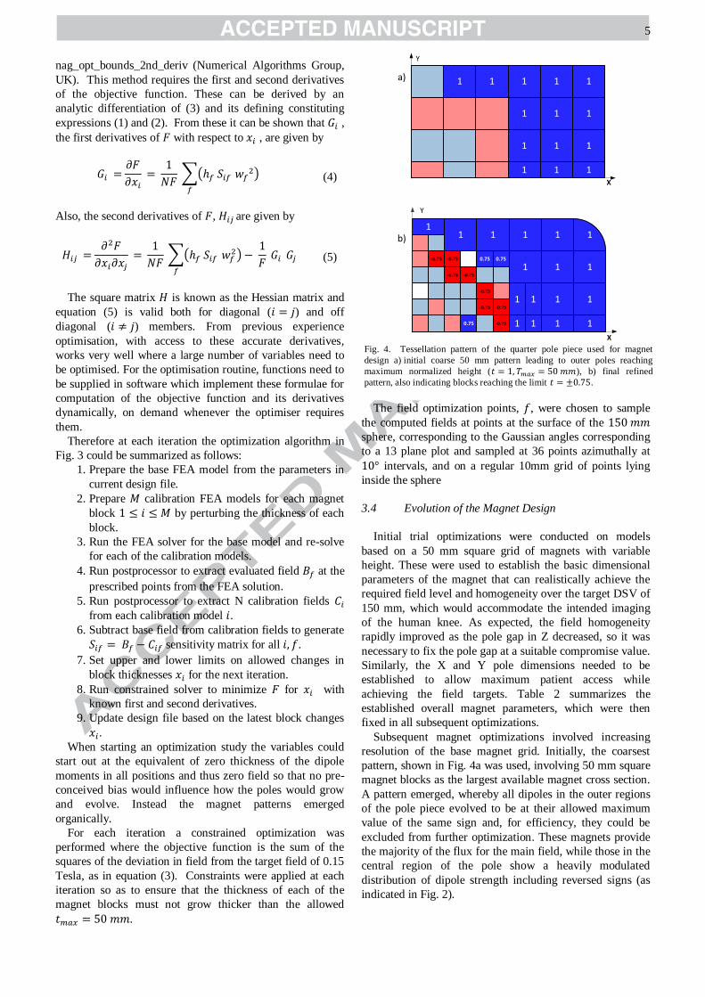
Subsequent magnet optimizations involved increasing

resolution of the base magnet grid. Initially, the coarsest

pattern, shown in Fig. 4a was used, involving 50 mm square

magnet blocks as the largest available magnet cross section.

A pattern emerged, whereby all dipoles in the outer regions

of the pole piece evolved to be at their allowed maximum

value of the same sign and, for efficiency, they could be

excluded from further optimization. These magnets provide

the majority of the flux for the main field, while those in the

central region of the pole show a heavily modulated

distribution of dipole strength including reversed signs (as

indicated in Fig. 2).

X

1 1 1 1

-0.75 0.75 0.75

1 1 1-0.75 -0.75

-0.75

1 1 1 1-0.75 -0.75

0.75 -0.75 1 1 1 1

1

-0.75

Y

1

11 1 1 1

1 1 1

1 1 1

1 1 1

Y

X

a)

b)

Fig. 4. Tessellation pattern of the quarter pole piece used for magnet

design a) initial coarse 50 mm pattern leading to outer poles reaching

maximum normalized height ( ), b) final refined

pattern, also indicating blocks reaching the limit .

6

It was found that in practice it was also beneficial to

impose a further constraint on the magnitude of change of

each variable for a single iteration. Failure to do so would

result in the field overshooting its target, due to the

nonlinearity of the steel and the complex interaction

between magnets and yoke. Therefore patience was needed

in gradually reducing this constraint on maximum amplitude

of change on each block from an initial 5 mm to as little as

0.1 mm per iteration.

In view of this, attempts were made to save the computing

time and reuse the calibrations more than once on the basis

that the parameter changes were very small. However this

approach was generally unsuccessful and often resulted in

the field quality deteriorating, highlighting the fact that with

iron present the process is highly nonlinear. Therefore the

magnet model and all its calibrations had to be refreshed

after each iteration.

After optimizing with the 50 mm square grid it was found

that the progress of field improvement had stalled, impeded

by the coarseness of this grid. Therefore the grid was refined

to 25 mm squares. With increased resolution, optimization

runs again established the dipoles in the outer regions of the

pole pieces that evolved to their maximum value, which

were then excluded from further iterations. In addition, it

was found that the corners of the poles were not contributing

significantly to the field and to keep the pole areas more

streamlined it was decided to fillet them along with the yoke

to a radius of one magnet block width or 50 mm. All this has

led to the final magnet pattern shown in Fig. 4b where 32

variables were modulated in the final optimization stages. A

typical model mesh comprised 1 million nodes and 6 million

elements. The computation for one complete iteration

including all calibrations was typically 3 hours on a Xeon

2.5 GHz, 2-processor PC with 96 Gb memory.

Additional optimization trials were made to assess the

effect of refining the squares by a further factor of 2 (to 12.5

mm squares). However, little tangible improvement in the

field quality seemed to accrue from this higher resolution,

while the number of variables quadrupled and the time taken

to re-run the FEA to obtain the calibrations became very

long (>10 hours). In addition the large number of such small

squares would make manufacture significantly more

difficult.

It was noticed during optimization that there was a

tendency for the magnitude of the modulated dipoles to be

mostly less than 0.75 (sometimes much less) on our

normalized scale, where . Therefore, to take

advantage of this effect, a constraint for all variable dipoles

was applied that they were only now allowed heights in the

range ± 0.75. This created a recess in the front face of the

pole of 0.25 (12.5 mm) and the optimizer was still able to

find as good a solution with this constraint in place. We

note that this emergent effect bears a resemblance to the

Rose ring feature on conventional magnet poles where the

thicker pole rim compensates for the truncation effect of the

edge of the pole and maintains a larger volume of uniform

field. The intention was to use the space that this recess

provided to house a light, low-profile passive shim set to

compensate for deviations in the field caused by

manufacturing and magnetisation tolerances without

impinging further on the net accessible gap of the magnet. It

was also discovered that the optimization led to two squares

in each quadrant to be very close to zero thickness, which

were then both constrained to zero and the remainder re-

optimized with no ill-effects on the field. These vacated

locations in the pole pieces later proved to be useful for

mechanically anchoring the shimset.

3.5 Permanent Magnet Grades

Table 2

Magnet dimensions fixed at the initial design stage

Parameter Dimension (mm)

Length in X 600

Width in Y 350

Clear gap between poles Z 220

Thickness of yoke 50

Thickness of magnet blocks (maximum) 50

7

Neodymium-Iron-Boron is available in many grades with

remanence ranging from around 1.2 to 1.425 Tesla, but with

the lower energy grades being available in harder versions –

that is, having a higher coercivity. In general the policy in

our magnet design was to use the highest grade N50 where

possible for maximum field strength but subject to the

magnetic intensity in the model not getting too close to

the coercivity of the material which might cause

demagnetization. By monitoring in the FEA models this

condition was found to be satisfied for the majority of the

magnets at their maximum values of thickness. However

where approached the specified value of coercivity a

harder grade was chosen (N48M or N48H) to give a larger

margin of safety against demagnetization. The trade-off is

that the harder grades are a little less strong and more

expensive through having more of the exotic rare earth

elements (e.g. dysprosium) in their composition. We note

that magnetic remanences in data sheets are not normally

specified with a precision better than 1% which we would

expect to lead to appreciable errors in fields measured in

ppm.

4. Results

4.1 Magnet Optimization

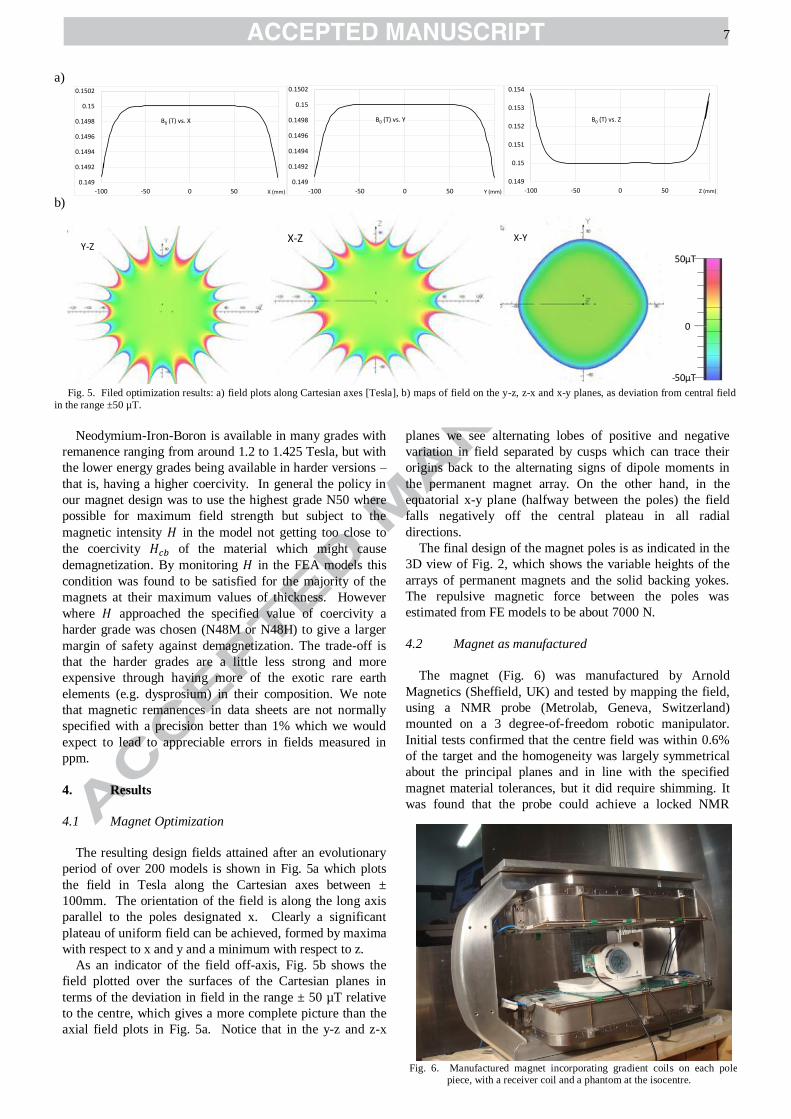
The resulting design fields attained after an evolutionary

period of over 200 models is shown in Fig. 5a which plots

the field in Tesla along the Cartesian axes between ±

100mm. The orientation of the field is along the long axis

parallel to the poles designated x. Clearly a significant

plateau of uniform field can be achieved, formed by maxima

with respect to x and y and a minimum with respect to z.

As an indicator of the field off-axis, Fig. 5b shows the

field plotted over the surfaces of the Cartesian planes in

terms of the deviation in field in the range ± 50 µT relative

to the centre, which gives a more complete picture than the

axial field plots in Fig. 5a. Notice that in the y-z and z-x

planes we see alternating lobes of positive and negative

variation in field separated by cusps which can trace their

origins back to the alternating signs of dipole moments in

the permanent magnet array. On the other hand, in the

equatorial x-y plane (halfway between the poles) the field

falls negatively off the central plateau in all radial

directions.

The final design of the magnet poles is as indicated in the

3D view of Fig. 2, which shows the variable heights of the

arrays of permanent magnets and the solid backing yokes.

The repulsive magnetic force between the poles was

estimated from FE models to be about 7000 N.

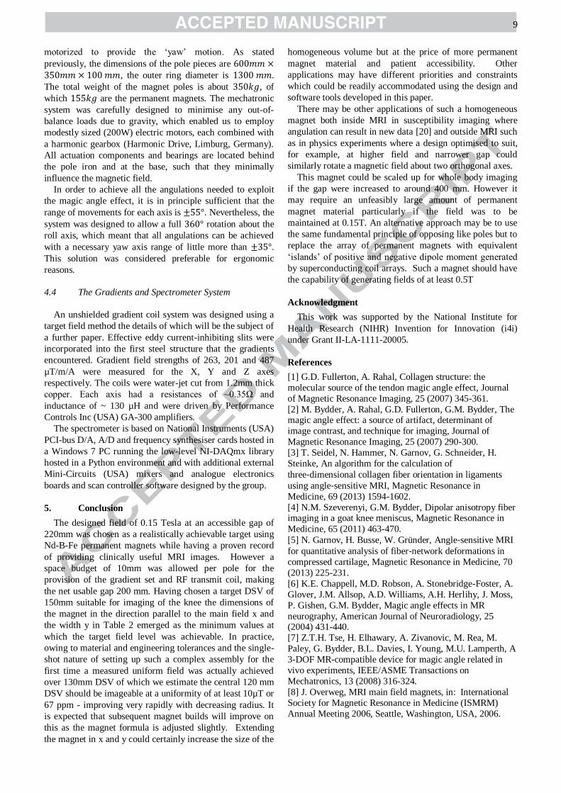
4.2 Magnet as manufactured

The magnet (Fig. 6) was manufactured by Arnold

Magnetics (Sheffield, UK) and tested by mapping the field,

using a NMR probe (Metrolab, Geneva, Switzerland)

mounted on a 3 degree-of-freedom robotic manipulator.

Initial tests confirmed that the centre field was within 0.6%

of the target and the homogeneity was largely symmetrical

about the principal planes and in line with the specified

magnet material tolerances, but it did require shimming. It

was found that the probe could achieve a locked NMR

a)

b)

Y-Z

X-Z

X-Y

50µT

-50µT

0

Fig. 5. Filed optimization results: a) field plots along Cartesian axes [Tesla], b) maps of field on the y-z, z-x and x-y planes, as deviation from central field

in the range ±50 µT.

0.149

0.1492

0.1494

0.1496

0.1498

0.15

0.1502

-100 -50 0 50 100X (mm)

B0 (T) vs. X

0.149

0.1492

0.1494

0.1496

0.1498

0.15

0.1502

-100 -50 0 50 100Y (mm)

B0 (T) vs. Y

0.149

0.15

0.151

0.152

0.153

0.154

-100 -50 0 50 100Z (mm)

B0 (T) vs. Z

Fig. 6. Manufactured magnet incorporating gradient coils on each pole

piece, with a receiver coil and a phantom at the isocentre.

8

signal at 75-80 mm from isocentre along the x and y axes

but no more than 65 mm along z. Therefore it was decided

to plot and optimise on a sphere of radius 65mm using 15

plane Gaussian angle plots, each sampled azimuthally at 24

points (15°).

A shim set was designed in the form of 4 plastic plates

per pole, designed to fit in the central recess of the magnet

face and providing an array of 1024 locations for mounting

5mm diameter button magnets in thicknesses between 1 and

5mm of either polarity. The shimming process involved five

iterations of field mapping and shim optimization using the

software described in Sec. 3.3 but slightly modified so the

objective function was the least-squares deviation from the

isocentre rather than the fixed target 0.15 Tesla thus

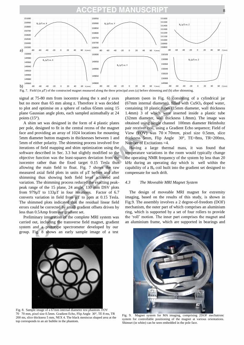
allowing the main field to float. Fig. 7 shows the raw

measured axial field plots in units of µT before and after

shimming thus showing both field level achieved and

variation. The shimming process reduced the exacting peak-

peak range of the 15 plane, 24 angle, 130 mm DSV plots

from 979µT to 133µT in four iterations. Factor of 6.7

converts variation in field from µT to ppm at 0.15 Tesla.

The shimmed plots indicated that the residual linear field

errors could be corrected by small gradient offsets driven by

less than 0.5Amp from our gradient set.

Preliminary integration of the complete MRI system was

carried out, including the transverse field magnet, gradient

system and a prototype spectrometer developed by our

group. Fig. 8 shows an early sample image of a test

phantom (seen in Fig. 6) consisting of a cylindrical jar

(67mm internal diameter), filled with CuSO4 doped water,

containing 10 plastic tubes (15mm diameter, wall thickness

1.4mm) 3 of which were inserted inside a plastic tube

(32mm diameter, wall thickness 1.8mm). The image was

obtained using single channel 100mm diameter Helmholtz

pair receiver coil, using a Gradient Echo sequence; Field of

View (FOV) was , pixel size 0.5mm, slice

thickness 5mm, Flip Angle 30°, TE=8ms, TR=200ms,

Number of Excitations =4.

Having a large thermal mass, it was found that

temperature variations in the room would typically change

the operating NMR frequency of the system by less than 20

kHz during an operating day which is well within the

capability of a B0 coil built into the gradient set designed to

compensate for such drift.

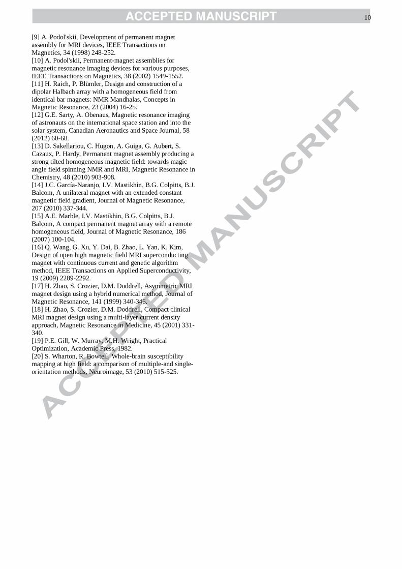
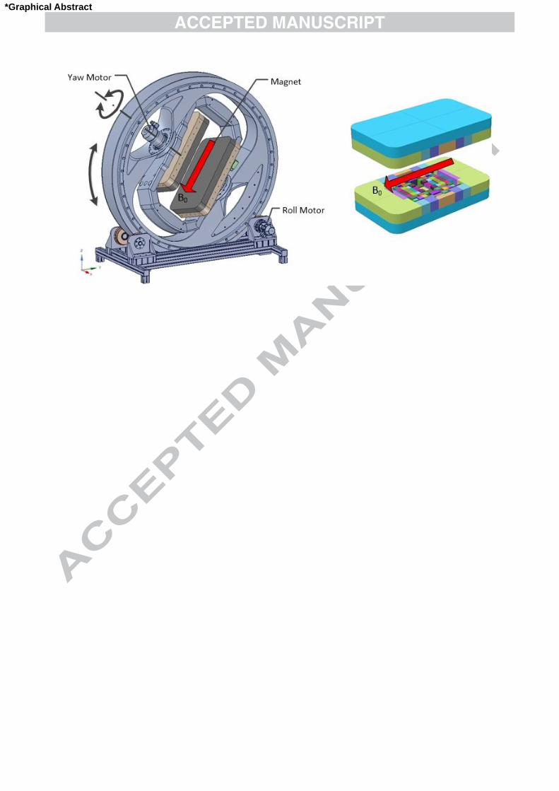
4.3 The Moveable MRI Magnet System

The design of moveable MRI magnet for extremity

imaging, based on the results of this study, is shown in

Fig.9. The assembly involves a 2 degree-of-freedom (DOF)

mechanism, the outer part of which comprises an aluminium

ring, which is supported by a set of four rollers to provide

the ‘roll’ motion. The inner part comprises the magnet and

an aluminium frame, which are supported in bearings and

a)

b) Fig. 7. Field (in ) of the constructed magnet measured along the three principal axes (a) before shimming and (b) after shimming.

150300

150400

150500

150600

150700

150800

150900

151000

-80 -60 -40 -20 0 20 40 60 80X (mm)

B0 (μT) vs. X

150650

150700

150750

150800

150850

150900

150950

-80 -60 -40 -20 0 20 40 60 80Y (mm)

B0 (μT) vs. Y

150800

150900

151000

151100

151200

151300

151400

151500

151600

-80 -60 -40 -20 0 20 40 60 80Z (mm)

B0 (μT) vs. Z

149860

149880

149900

149920

149940

149960

149980

150000

-80 -60 -40 -20 0 20 40 60 80X (mm)

B0 (μT) vs. X

149800

149850

149900

149950

150000

-80 -60 -40 -20 0 20 40 60 80Y (mm)

B0 (μT) vs. Y

149980

150000

150020

150040

150060

150080

150100

-80 -60 -40 -20 0 20 40 60 80Z (mm)

B0 (μT) vs. Z

Fig. 8. Sample image of a 67mm internal diameter test phantom. FOV

70 70 mm, pixel size 0.5mm. Gradient Echo, Flip Angle 30°, TE 8 ms, TR

200 ms, slice thickness 5 mm, NEX 4. The black meniscus shaped area at thetop corresponds to an air bubble in the phantom.

Fig. 9. Magnet system for MA imaging, comprising 2DOF mechatronc

system for controllable positioning of the magnet at various orientations.Shimset (in white) can be seen embedded in the pole face.

9

motorized to provide the ‘yaw’ motion. As stated

previously, the dimensions of the pole pieces are , the outer ring diameter is .

The total weight of the magnet poles is about , of

which are the permanent magnets. The mechatronic

system was carefully designed to minimise any out-of-

balance loads due to gravity, which enabled us to employ

modestly sized (200W) electric motors, each combined with

a harmonic gearbox (Harmonic Drive, Limburg, Germany).

All actuation components and bearings are located behind

the pole iron and at the base, such that they minimally

influence the magnetic field.

In order to achieve all the angulations needed to exploit

the magic angle effect, it is in principle sufficient that the

range of movements for each axis is . Nevertheless, the

system was designed to allow a full rotation about the

roll axis, which meant that all angulations can be achieved

with a necessary yaw axis range of little more than . This solution was considered preferable for ergonomic

reasons.

4.4 The Gradients and Spectrometer System

An unshielded gradient coil system was designed using a

target field method the details of which will be the subject of

a further paper. Effective eddy current-inhibiting slits were

incorporated into the first steel structure that the gradients

encountered. Gradient field strengths of 263, 201 and 487

µT/m/A were measured for the X, Y and Z axes

respectively. The coils were water-jet cut from 1.2mm thick

copper. Each axis had a resistances of ~0.35Ω and

inductance of ~ 130 µH and were driven by Performance

Controls Inc (USA) GA-300 amplifiers.

The spectrometer is based on National Instruments (USA)

PCI-bus D/A, A/D and frequency synthesiser cards hosted in

a Windows 7 PC running the low-level NI-DAQmx library

hosted in a Python environment and with additional external

Mini-Circuits (USA) mixers and analogue electronics

boards and scan controller software designed by the group.

5. Conclusion

The designed field of 0.15 Tesla at an accessible gap of

220mm was chosen as a realistically achievable target using

Nd-B-Fe permanent magnets while having a proven record

of providing clinically useful MRI images. However a

space budget of 10mm was allowed per pole for the

provision of the gradient set and RF transmit coil, making

the net usable gap 200 mm. Having chosen a target DSV of

150mm suitable for imaging of the knee the dimensions of

the magnet in the direction parallel to the main field x and

the width y in Table 2 emerged as the minimum values at

which the target field level was achievable. In practice,

owing to material and engineering tolerances and the single-

shot nature of setting up such a complex assembly for the

first time a measured uniform field was actually achieved

over 130mm DSV of which we estimate the central 120 mm

DSV should be imageable at a uniformity of at least 10µT or

67 ppm - improving very rapidly with decreasing radius. It

is expected that subsequent magnet builds will improve on

this as the magnet formula is adjusted slightly. Extending

the magnet in x and y could certainly increase the size of the

homogeneous volume but at the price of more permanent

magnet material and patient accessibility. Other

applications may have different priorities and constraints

which could be readily accommodated using the design and

software tools developed in this paper.

There may be other applications of such a homogeneous

magnet both inside MRI in susceptibility imaging where

angulation can result in new data [20] and outside MRI such

as in physics experiments where a design optimised to suit,

for example, at higher field and narrower gap could

similarly rotate a magnetic field about two orthogonal axes.

This magnet could be scaled up for whole body imaging

if the gap were increased to around 400 mm. However it

may require an unfeasibly large amount of permanent

magnet material particularly if the field was to be

maintained at 0.15T. An alternative approach may be to use

the same fundamental principle of opposing like poles but to

replace the array of permanent magnets with equivalent

‘islands’ of positive and negative dipole moment generated

by superconducting coil arrays. Such a magnet should have

the capability of generating fields of at least 0.5T

Acknowledgment

This work was supported by the National Institute for

Health Research (NIHR) Invention for Innovation (i4i)

under Grant II-LA-1111-20005.

References

[1] G.D. Fullerton, A. Rahal, Collagen structure: the

molecular source of the tendon magic angle effect, Journal

of Magnetic Resonance Imaging, 25 (2007) 345-361.

[2] M. Bydder, A. Rahal, G.D. Fullerton, G.M. Bydder, The magic angle effect: a source of artifact, determinant of

image contrast, and technique for imaging, Journal of

Magnetic Resonance Imaging, 25 (2007) 290-300.

[3] T. Seidel, N. Hammer, N. Garnov, G. Schneider, H.

Steinke, An algorithm for the calculation of

three‐dimensional collagen fiber orientation in ligaments

using angle‐sensitive MRI, Magnetic Resonance in

Medicine, 69 (2013) 1594-1602.

[4] N.M. Szeverenyi, G.M. Bydder, Dipolar anisotropy fiber imaging in a goat knee meniscus, Magnetic Resonance in

Medicine, 65 (2011) 463-470.

[5] N. Garnov, H. Busse, W. Gründer, Angle‐sensitive MRI

for quantitative analysis of fiber‐network deformations in

compressed cartilage, Magnetic Resonance in Medicine, 70

(2013) 225-231.

[6] K.E. Chappell, M.D. Robson, A. Stonebridge-Foster, A.

Glover, J.M. Allsop, A.D. Williams, A.H. Herlihy, J. Moss,

P. Gishen, G.M. Bydder, Magic angle effects in MR

neurography, American Journal of Neuroradiology, 25 (2004) 431-440.

[7] Z.T.H. Tse, H. Elhawary, A. Zivanovic, M. Rea, M.

Paley, G. Bydder, B.L. Davies, I. Young, M.U. Lamperth, A

3-DOF MR-compatible device for magic angle related in

vivo experiments, IEEE/ASME Transactions on

Mechatronics, 13 (2008) 316-324.

[8] J. Overweg, MRI main field magnets, in: International

Society for Magnetic Resonance in Medicine (ISMRM)

Annual Meeting 2006, Seattle, Washington, USA, 2006.

10

[9] A. Podol'skii, Development of permanent magnet

assembly for MRI devices, IEEE Transactions on

Magnetics, 34 (1998) 248-252.

[10] A. Podol'skii, Permanent-magnet assemblies for

magnetic resonance imaging devices for various purposes,

IEEE Transactions on Magnetics, 38 (2002) 1549-1552.

[11] H. Raich, P. Blümler, Design and construction of a

dipolar Halbach array with a homogeneous field from

identical bar magnets: NMR Mandhalas, Concepts in Magnetic Resonance, 23 (2004) 16-25.

[12] G.E. Sarty, A. Obenaus, Magnetic resonance imaging

of astronauts on the international space station and into the

solar system, Canadian Aeronautics and Space Journal, 58

(2012) 60-68.

[13] D. Sakellariou, C. Hugon, A. Guiga, G. Aubert, S.

Cazaux, P. Hardy, Permanent magnet assembly producing a

strong tilted homogeneous magnetic field: towards magic

angle field spinning NMR and MRI, Magnetic Resonance in

Chemistry, 48 (2010) 903-908.

[14] J.C. García-Naranjo, I.V. Mastikhin, B.G. Colpitts, B.J. Balcom, A unilateral magnet with an extended constant

magnetic field gradient, Journal of Magnetic Resonance,

207 (2010) 337-344.

[15] A.E. Marble, I.V. Mastikhin, B.G. Colpitts, B.J.

Balcom, A compact permanent magnet array with a remote

homogeneous field, Journal of Magnetic Resonance, 186

(2007) 100-104.

[16] Q. Wang, G. Xu, Y. Dai, B. Zhao, L. Yan, K. Kim,

Design of open high magnetic field MRI superconducting

magnet with continuous current and genetic algorithm

method, IEEE Transactions on Applied Superconductivity, 19 (2009) 2289-2292.

[17] H. Zhao, S. Crozier, D.M. Doddrell, Asymmetric MRI

magnet design using a hybrid numerical method, Journal of

Magnetic Resonance, 141 (1999) 340-346.

[18] H. Zhao, S. Crozier, D.M. Doddrell, Compact clinical

MRI magnet design using a multi‐layer current density

approach, Magnetic Resonance in Medicine, 45 (2001) 331-

340.

[19] P.E. Gill, W. Murray, M.H. Wright, Practical

Optimization, Academic Press, 1982.

[20] S. Wharton, R. Bowtell, Whole-brain susceptibility mapping at high field: a comparison of multiple-and single-

orientation methods, Neuroimage, 53 (2010) 515-525.

*Graphical Abstract

11

A Permanent MRI Magnet for Magic Angle Imaging

Having its Field Parallel to the Poles

Highlights

· Novel open magnet design having field parallel to the poles.

· Magnet suitable for human in-vivo MRI studies of the magic angle effect.

· 3D modelling and optimization method using specially developed software for configuration control, dealing with large number of parameters.

· Magnet performance verified by field measurements made on the manufactured magnet.

· High quality MR imaging demonstrated following integration of the magnet with MRI system.