Embed Size (px)
Citation preview
Master Thesis Electrical Engineering April 2015
A Performance Study of VM Live Migration over the WAN
TAHA MOHAMMAD CHANDRA SEKHAR EATI
Department of Communication Systems Blekinge Institute of Technology SE-371 79 Karlskrona Sweden
This thesis is submitted to the School of Computing at Blekinge Institute of Technology inpartial fulfillment of the requirements for the degree of Master of Science in ElectricalEngineering on Telecommunication Systems. The thesis is equivalent to 40 weeks of full timestudies.
Contact Information: Author(s): Taha Mohammad, Chandra Sekhar Eati. E-mail: [email protected], [email protected].
University Examiner(s): Prof. Kurt Tutschku, Department of Communication Systems.
University advisor(s): Dr. Dragos Ilie, Department of Communication Systems.
School of Computing Blekinge Institute of Technology SE-371 79 Karlskrona Sweden
Internet : www.bth.se Phone : +46 455 38 50 00 Fax : +46 455 38 50 57
Abstract
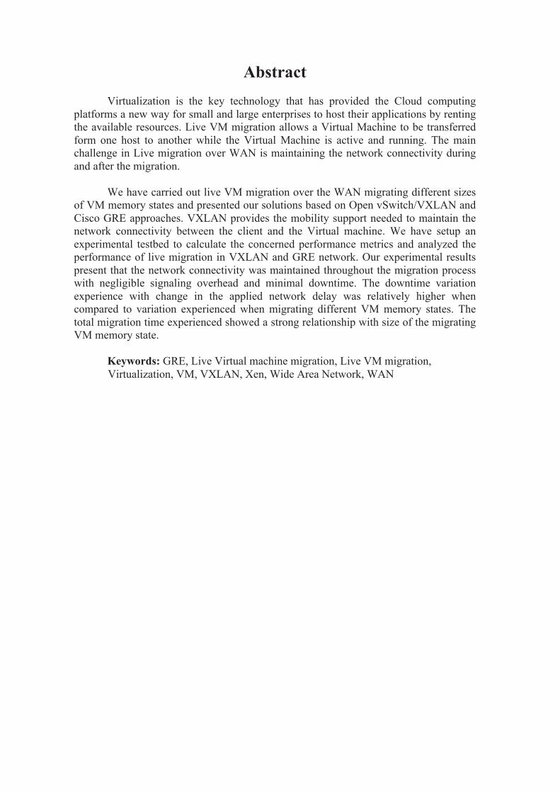
Virtualization is the key technology that has provided the Cloud computing platforms a new way for small and large enterprises to host their applications by renting the available resources. Live VM migration allows a Virtual Machine to be transferred form one host to another while the Virtual Machine is active and running. The main challenge in Live migration over WAN is maintaining the network connectivity during and after the migration.
We have carried out live VM migration over the WAN migrating different sizes
of VM memory states and presented our solutions based on Open vSwitch/VXLAN and Cisco GRE approaches. VXLAN provides the mobility support needed to maintain the network connectivity between the client and the Virtual machine. We have setup an experimental testbed to calculate the concerned performance metrics and analyzed the performance of live migration in VXLAN and GRE network. Our experimental results present that the network connectivity was maintained throughout the migration process with negligible signaling overhead and minimal downtime. The downtime variation experience with change in the applied network delay was relatively higher when compared to variation experienced when migrating different VM memory states. The total migration time experienced showed a strong relationship with size of the migrating VM memory state.
Keywords: GRE, Live Virtual machine migration, Live VM migration,
Virtualization, VM, VXLAN, Xen, Wide Area Network, WAN

Acknowledgments
We would like to firstly thank the Almighty God for blessing us with knowledge,
strength and guidance. We would also like to thank our beloved parents and other family members for the unconditional support and love. They are always with us.
We are deeply graceful to our supervisor, Dr. Dragos Ilie, for his help,
encouragement and support through out the thesis work with valuable suggestions. We had learnt a lot in the entire process from various meeting and crucial discussions with him, which also helps us in future careers. He also helped us by providing feedback during the meeting which is the crucial part for the successful completion of our Master thesis, which also helped us in following the right track. Therefore, it is our great pleasure to thank him and express our heartfelt appreciation for his guidance and support.
Our next gratitude goes to Dr. Anders Nelsson and Dr. Yuriy Andrushko for
lending us lab rooms and Cisco hardware routers for our experiment, which was one of the vital elements in our laboratory test-bed. Furthermore, we would like to thank Prof. Dr. Kurt Tutschku for his useful suggestions and motivation through out the study process of master thesis.
Last but not the least, we would like to thank all our classmates and cheerful
group of friends (Amulya, Kamal, Sansank, Umesh and Pawan) for their encouragement towards us. We have shared lots of precious moments with them through out a year in Sweden. We will be forever grateful for all your love and help and we wish you all the best.
Mohammad Taha & Chandra Sekhar Eati
Karlskrona, April 2015
LIST OF CONTENTS
LIST OF FIGURES
1. Xen Migration Time Line [4] ............................................................................................ 8
2. Xen Architecture [10] ...................................................................................................... 13
3. Virtual interfaces (VIFs) and Physical interfaces (PIFs) interconnected via a Virtual switch .............................................................................................................................. 14
4. VXLAN Packet Format [32] ........................................................................................... 21
5. Live VM Migration using VXLAN/GRE approach ........................................................ 22
6. Inter VM communications and migration for hosts in different L2 subnets [9] ............. 25
7. Cisco PE-PE tunneling .................................................................................................... 26
8. PDF and CDF plot of Pareto distribution ........................................................................ 27
9. Testbed (Open vSwitch & VXLAN) ............................................................................... 30
10. Testbed (Cisco GRE tunneling) ...................................................................................... 31
11. Downtime variation with variable delay (256M VM memory) ...................................... 37
12. Downtime variation with variable delay (512M VM memory) ...................................... 38
13. Downtime variation with variable delay (1024M VM memory) .................................... 39
14. Total Migration time variation with variable delay (256M VM memory) ...................... 40
15. Total Migration time variation with variable delay (512M VM memory) ...................... 41
16. Total Migration time variation with variable delay (1024M VM memory) .................... 42
17. Comparison of VXLAN with GRE approach over network delay migrating 256MB VM memory ............................................................................................................................ 45
18. Comparison of VXLAN with GRE approach over network delay migrating 512 MB VM memory ............................................................................................................................ 46
19. Comparison of VXLAN with GRE approach over network delay migrating 1024 MB VM memory .................................................................................................................... 47
20. Comparison of VXLAN with GRE approach over network delay migrating 256 MB VM memory ............................................................................................................................ 48
21. Comparison of VXLAN with GRE approach over network delay migrating 512 MB VM memory ............................................................................................................................ 49
22. Comparison of VXLAN with GRE approach over network delay migrating 1024 MB VM memory .................................................................................................................... 50
23. Comparison of VXLAN with GRE approach over network delay migrating different VM memory sizes ........................................................................................................... 51
24. Network overhead comparison of VXLAN and GRE, migrating 256 MB VM memory 53
25. Network overhead comparison of VXLAN and GRE, migrating 512 MB VM memory 54
26. Network overhead comparison of VXLAN and GRE, migrating 1024 MB VM memory ......................................................................................................................................... 54
27. Provider-Edge to Provider-Edge tunneling ..................................................................... 63
28. PDF and CDF of Pareto distribution for 30 ms delay and 6 ms jitter ............................. 66

LIST OF EQUATIONS
PDF function for the generalized Pareto distribution .......................................... 27 Confidence Interval ............................................................................................. 35
3. Relative Error ....................................................................................................... 35
LIST OF TABLES
1. Downtime migrating 256 MB VM memory at variable network delays ........ 36 2. Downtime migrating 512 MB VM memory at variable network delays ........ 37
3. Downtime migrating 1024 MB VM memory at variable network delays ...... 38 4. Total Migration time for 256 MB VM memory state at variable network delay
......................................................................................................................... 40 5. Total Migration time for 512 MB VM memory state at variable network delay
......................................................................................................................... 41 6. Total Migration time for 1024 MB VM memory state at variable network
delay ................................................................................................................ 42 7. Downtime migrating 256 MB VM memory at variable network delays ........ 44
8. Downtime migrating 512 MB VM memory at variable network delays ........ 45 9. Downtime migrating 1024 MB VM memory at variable network delays ...... 46
10. Migration time migrating 256 MB VM memory at variable network delays . 48 11. Migration time migrating 512 MB VM memory at variable network delays . 49
12. Migration time migrating 1024 MB VM memory at variable network delays50 13. iSCSI IP address Details ................................................................................. 56
Acronyms ABSS Activity Bases Sector Synchronization MIPv6 Mobile Internet Protocol version 6
ARP Address Resolution Protocol NIC Network Interface Card
BGP Border Gateway Protocol
OS Operating System
CAM Content Addressable Memory
OSPF Open Shortest Path First
CBR Content Based Redundancy
PE Provider Edge
CE Customer Edge
PIF Physical Interface
CPU Central Processing Unit
PMIPv6 Proxy Mobile Internet Protocol version 6
DC Data Center
RARP Reverse Address Resolution Protocol
DDNS Dynamic Domain Name Service
RIP Routing Information Protocol
DNS Domain Name Service
SSH Secure Socket Shell
DRBD Distributed Replicated Block Device TCP Transmission Control Protocol
GRE Generic Routing Encapsulation
UDP User Datagram Protocol
IO Input Output
VDE Virtual Distributed Ethernet
IPSec Internet Protocol Security
VIF Virtual Interface
IPv4 Internet Protocol version 4
VLAN Virtual Local Area Network
IPv6 Internet Protocol version 6
VM Virtual Machine
ISCSI Internet Small Computer System Interface
VMM Virtual Machine Monitor
KVM Kernel-based Virtual Machine
VMTC Virtual Machine Traffic Controller
LAN Local Area Network
VNI VXLAN Network Identifier
LTS Long Term Service
VPN Virtual Private Network
LVM Logical Volume Manager
VTEP VXLAN Tunnel End Point
MAN Metropolitan Area Network
VXLAN Virtual Extensible Local Area Network
MBPS Mega Bytes per Second WAN Wide Area Network
1
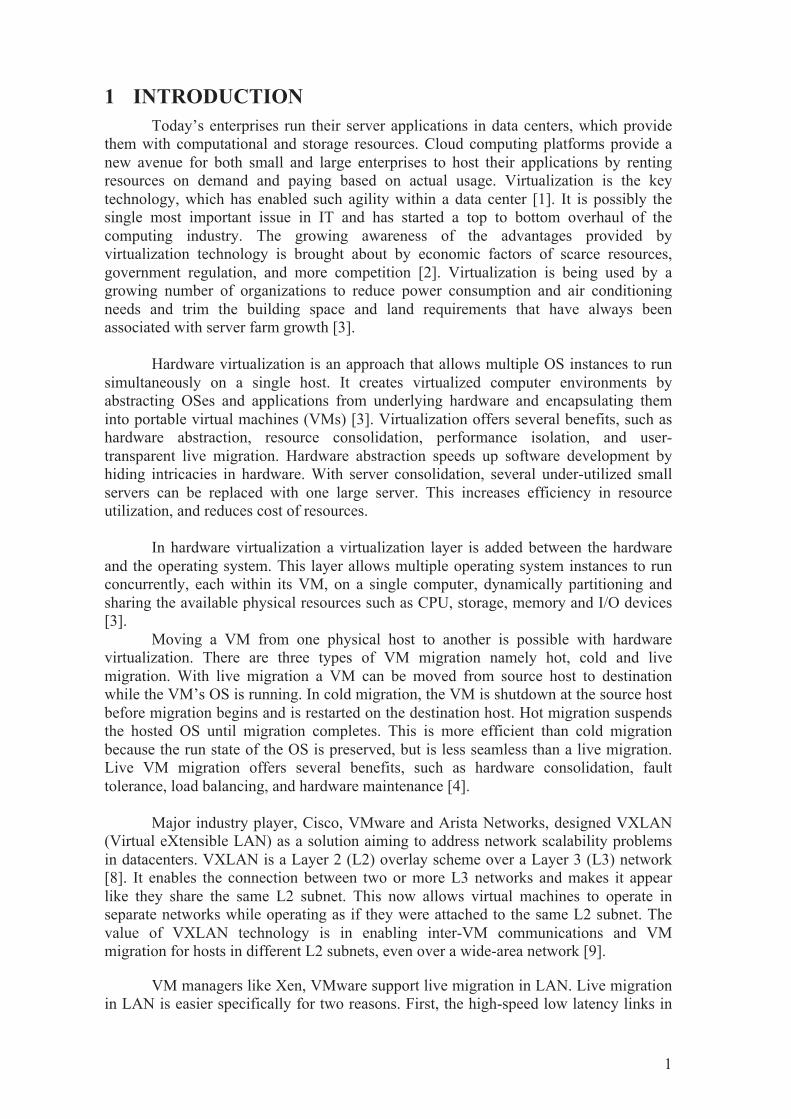
1 INTRODUCTION Today’s enterprises run their server applications in data centers, which provide
them with computational and storage resources. Cloud computing platforms provide a new avenue for both small and large enterprises to host their applications by renting resources on demand and paying based on actual usage. Virtualization is the key technology, which has enabled such agility within a data center [1]. It is possibly the single most important issue in IT and has started a top to bottom overhaul of the computing industry. The growing awareness of the advantages provided by virtualization technology is brought about by economic factors of scarce resources, government regulation, and more competition [2]. Virtualization is being used by a growing number of organizations to reduce power consumption and air conditioning needs and trim the building space and land requirements that have always been associated with server farm growth [3].
Hardware virtualization is an approach that allows multiple OS instances to run
simultaneously on a single host. It creates virtualized computer environments by abstracting OSes and applications from underlying hardware and encapsulating them into portable virtual machines (VMs) [3]. Virtualization offers several benefits, such as hardware abstraction, resource consolidation, performance isolation, and user-transparent live migration. Hardware abstraction speeds up software development by hiding intricacies in hardware. With server consolidation, several under-utilized small servers can be replaced with one large server. This increases efficiency in resource utilization, and reduces cost of resources.
In hardware virtualization a virtualization layer is added between the hardware
and the operating system. This layer allows multiple operating system instances to run concurrently, each within its VM, on a single computer, dynamically partitioning and sharing the available physical resources such as CPU, storage, memory and I/O devices [3].
Moving a VM from one physical host to another is possible with hardware virtualization. There are three types of VM migration namely hot, cold and live migration. With live migration a VM can be moved from source host to destination while the VM’s OS is running. In cold migration, the VM is shutdown at the source host before migration begins and is restarted on the destination host. Hot migration suspends the hosted OS until migration completes. This is more efficient than cold migration because the run state of the OS is preserved, but is less seamless than a live migration. Live VM migration offers several benefits, such as hardware consolidation, fault tolerance, load balancing, and hardware maintenance [4].
Major industry player, Cisco, VMware and Arista Networks, designed VXLAN
(Virtual eXtensible LAN) as a solution aiming to address network scalability problems in datacenters. VXLAN is a Layer 2 (L2) overlay scheme over a Layer 3 (L3) network [8]. It enables the connection between two or more L3 networks and makes it appear like they share the same L2 subnet. This now allows virtual machines to operate in separate networks while operating as if they were attached to the same L2 subnet. The value of VXLAN technology is in enabling inter-VM communications and VM migration for hosts in different L2 subnets, even over a wide-area network [9].
VM managers like Xen, VMware support live migration in LAN. Live migration in LAN is easier specifically for two reasons. First, the high-speed low latency links in
Section 1 – INTRODUCTION
2
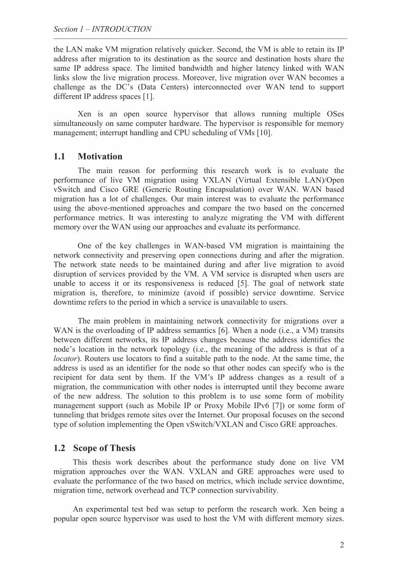
the LAN make VM migration relatively quicker. Second, the VM is able to retain its IP address after migration to its destination as the source and destination hosts share the same IP address space. The limited bandwidth and higher latency linked with WAN links slow the live migration process. Moreover, live migration over WAN becomes a challenge as the DC’s (Data Centers) interconnected over WAN tend to support different IP address spaces [1].
Xen is an open source hypervisor that allows running multiple OSes simultaneously on same computer hardware. The hypervisor is responsible for memory management; interrupt handling and CPU scheduling of VMs [10].
1.1 Motivation The main reason for performing this research work is to evaluate the
performance of live VM migration using VXLAN (Virtual Extensible LAN)/Open vSwitch and Cisco GRE (Generic Routing Encapsulation) over WAN. WAN based migration has a lot of challenges. Our main interest was to evaluate the performance using the above-mentioned approaches and compare the two based on the concerned performance metrics. It was interesting to analyze migrating the VM with different memory over the WAN using our approaches and evaluate its performance.
One of the key challenges in WAN-based VM migration is maintaining the
network connectivity and preserving open connections during and after the migration. The network state needs to be maintained during and after live migration to avoid disruption of services provided by the VM. A VM service is disrupted when users are unable to access it or its responsiveness is reduced [5]. The goal of network state migration is, therefore, to minimize (avoid if possible) service downtime. Service downtime refers to the period in which a service is unavailable to users.
The main problem in maintaining network connectivity for migrations over a
WAN is the overloading of IP address semantics [6]. When a node (i.e., a VM) transits between different networks, its IP address changes because the address identifies the node’s location in the network topology (i.e., the meaning of the address is that of a locator). Routers use locators to find a suitable path to the node. At the same time, the address is used as an identifier for the node so that other nodes can specify who is the recipient for data sent by them. If the VM’s IP address changes as a result of a migration, the communication with other nodes is interrupted until they become aware of the new address. The solution to this problem is to use some form of mobility management support (such as Mobile IP or Proxy Mobile IPv6 [7]) or some form of tunneling that bridges remote sites over the Internet. Our proposal focuses on the second type of solution implementing the Open vSwitch/VXLAN and Cisco GRE approaches.
1.2 Scope of Thesis This thesis work describes about the performance study done on live VM
migration approaches over the WAN. VXLAN and GRE approaches were used to evaluate the performance of the two based on metrics, which include service downtime, migration time, network overhead and TCP connection survivability.
An experimental test bed was setup to perform the research work. Xen being a
popular open source hypervisor was used to host the VM with different memory sizes.
Section 1 – INTRODUCTION
3
Various tools such as NetEm (Network Emulator), NTP (Network Time Protocol), t-shark were used to facilitate the research. Open vSwitch/VXLAN and GRE tunneling were configured on the Linux system and Cisco routers respectively to implement the two above-mentioned approaches. Moreover, the results obtained from both the approaches were analyzed and compared.
1.3 Virtualization The term virtualization defines the separation of a service request from the
physical delivery of that service. It was first introduced when the mainframes of the 1960’s and 1970’s were logically partitioned to allow concurrent execution of multiple applications on the same mainframe hardware [11]. Moderately, it became popular and grabbed attention from the industry and academia. This technology today allows running multiple operating systems on the same physical host.
In simple terms, Virtualization is a framework or methodology of dividing the
resources of a computer into multiple execution environments, by applying one or more concepts or technologies such as hardware and software partitioning, time-sharing, partial or complete machine simulation, emulation, quality of service, and many others. [12]
A virtualization layer is added between the hardware and the operating system. This layer allows multiple OS instances within VM’s to run concurrently on a single computer, dynamically partitioning and sharing the available resources such as CPU, memory, storage and I/O devices.
In x86 systems, virtualization approaches use either hosted or hypervisor
architecture. A hosted architecture runs the virtualization layer as an application on top of OS whereas in case of a hypervisor (bare metal) architecture a virtualization layer is installed directly on a fresh x86 based system. A hypervisor is more efficient than hosted architecture since it has direct access to the hardware resources unlike in hosted architecture, which runs on top of the OS.
x86 OSes were designed to run on the bare metal directly and thus it presented
some key challenge in hardware virtualization. x86 architecture provides four levels of privilege to OSes. These levels range from 0 to 3 and are often described as protection rings. Privilege level 0 (Ring 0) is the most privileged one while privilege level 3 (Ring 3) is the least privileged. OSes need to execute their privileged instructions in Ring 0 as they need to have direct access to computer resources [3].
1.3.1 Components of Virtualization There are two main components of virtualization: Hypervisor and Guest (or
VM). i) Hypervisor – The hypervisor is also termed as virtualization layer, which is
a software layer that manages and hosts the VM’s. There are two categories of hypervisors, based on architecture: • Type 1 – It is a native or bare metal hypervisor that runs directly on the
host hardware. Thus it has direct access to the hardware resources and handles allocation of resources to guests as well. Some hypervisors require a privileged guest such as Domain-0 or Dom0 to provide
Section 1 – INTRODUCTION
4
management interface for the hypervisor. Xen and VMware ESX are some common examples of such type of hypervisors.
• Type 2 – It is also called as hosted hypervisor as it is installed and run on
top of a hosting OS. This type of hypervisor has an advantage that it has fewer hardware/driver issues, since the host OS is responsible for interfacing with the hardware. Nonetheless, it performs lower as compared to type 1 hypervisor due to overhead caused by the host OS. Virtual Box and VMware Workstation are examples of such hypervisors [13].
ii) Guest - The guest is a virtualized environment with its own OS and
applications. It runs on top of the hypervisor. The guest may run a native OS or a modified version of the OS depending on the capabilities of the hypervisor and hardware.
1.3.2 Techniques of Virtualization:
There are three different techniques of virtualization [3]. Xen supports two types of virtualization namely Paravirtualization and Hardware-assisted virtualization.
a) Full Virtualization – Full Virtualization can be achieved using the
combination of binary translation and direct execution as the guest OS is fully abstracted by the virtualization layer from the underlying layer. The guest OS is not aware of it being virtualized and thus requires no modification. It requires no hardware assist or operating system assist to virtualize sensitive and privileged instructions. The aim of this technique is to create VMs that perform in a way real machines perform [14]. It requires virtualizing the components such as Disk and network devices, Interrupts and timers, Legacy boot, Privileged instructions and memory.
Full Virtualization offers the best isolation and security for virtual machines,
and thus simplifies migration and portability as the same guest OS instance can run virtualized or on native hardware [3]. VMware’s virtualization products and Microsoft Virtual Server are common examples of this virtualization technique.
b) Paravirtualization – is a lightweight virtualization technique that requires
modification of the guest OS for better efficiency [10]. Xen achieves CPU virtualization in x86 systems by modifying the guest OS to run in a less privileged ring and uses hypercalls (i.e., functions calls handled by the hypervisor) and events to transfer the control between the hypervisor and the guest. Moreover hypercalls are used to pass page table update requests to the hypervisor [15].
Paravirtualization differs from full virtualization in a way, where the unmodified OS is not aware of it being virtualized and sensitive OS calls are trapped using binary translation. In terms of its value Proposition, Paravirtualization has lower virtualization overhead whereas in terms of performance advantage over full virtualization can vary depending on the workload. The open source Xen project is an example of such virtualization technique where the processor and memory is virtualized using a modified Linux kernel and the I/O using custom guest OS drivers [3].
Section 1 – INTRODUCTION
5
c) Hardware assisted virtualization – is a virtualization technique that allows
guests to run unmodified OS by making use of special features offered by hardware. Enhancements have been made by the hardware vendors to target privileged instructions with a new CPU execution mode feature, which allows the VMM to run in a new mode below Ring 0.
In this virtualization technique, privileged and sensitive calls are set to automatically trap to the hypervisor. Thus there arises no need of either binary translation or Paravirtualization [3]. In most of the circumstances, VMware’s binary translation approach currently outperforms the first generation hardware-assist implementations.
Given the emerging applications and Future Internet services, network operators are looking for network virtualization approaches to effectively share their network infrastructure [16]. The main focus of this thesis is to investigate the use of GRE tunnel using Cisco Routers and VXLAN tunnel using Linux systems to support live VM migration across WAN and then compare its performance based on its performance metrics towards live VM migration.
1.4 Live VM Migration Live VM Migration can be performed based on two basic network scenarios:
Local Area Network (LAN) and Wide Area Network (WAN). Live Migration over LAN is easier for two reasons. Firstly, because of the high-
speed low-latency links in the LAN which makes migration comparatively quicker. Secondly, as the VM can retain its IP address (es) after migration since the hosts share the same IP address space.
Migration across LAN/WAN consists of four components: • Migrating the CPU • Migrating the memory • Migrating the disk • Migrating the network state of the VM. Live Migration over WAN has some challenges to be met. Relatively higher
latency and limited bandwidth are the root causes for slow live migration across a WAN. Moreover, WAN-based live migration would entail change in VM’s IP address(es) as Data Centers interconnected in a WAN tend to support different IP address spaces [1].
1.4.1 Live Migration over WAN A Virtual Machine Migration over the WAN (Internet) involves moving the VM
from a physical host residing in one network to another host residing in another network.
The CPU state is defined by the actual contents of the CPU registers and the state of the underlying OS which includes parameters related to processes, memory and file management. In practical VM migration implementations, the CPU state migration is often encapsulated inside memory state migration. Xen migrates the CPU state during its final stage of its memory state migration [17].
Section 1 – INTRODUCTION
6
1.4.2 Benefits of Live VM Migration
VMware and Xen both have centralized VM monitoring and management facilities. With the help of these facilities, VM’s can be readily moved from one hardware cluster to another in Data Centers within a LAN. DC’s in general are all benefited from the merits of live VM migration such as load balancing and server consolidation. Nonetheless, WAN’s are not benefited from Live VM migration since the scope of current live migration practice is limited to LAN situations only.
The following lists down some of the potential advantages of WAN established
Live VM migration across subnets [1]: • Consolidation – In order to save the cost of resources and improve power
consumption efficiency, several underutilized small data centers can be replaced with few larger ones. Such unification requires moving applications and data from one data center to another in VM containers across WAN.
• Load balancing – This is one of the important issues to deal with WAN based VM migration. It requires the transfer of VM’s from an overloaded host to a light loaded ones.
• Scaling – Multiple sites need to be created at different geographical sites to scale up as the cloud grows. Thus, migration of VM’s across DC’s would be required to allow load balancing and consolidation activities.
• Disaster recovery and reliability – In times of catastrophe or any fault occurrence, disaster recovery operation requires moving VM from one hardware cluster to another. In such cases, VM’s can be migrated to mirrored sites across cloud with minimal downtime.
• Follow-the-sun – It is an IT strategy designed for project teams that can span multiple continents. In this strategy, tasks are passed around daily between sites that are separated by the big time zones. At the end of the day, applications and data will be moved from one site to another.
• Maintenance – When it comes to maintenance, a need arises to maintain computer hardware. Applications and data can be migrated to another machine in VM containers to free up the hardware for maintenance
7
2 BACKGROUND 2.1 Components of Migration 2.1.1 Memory State Migration
Migrating the memory state of VM consists of moving the VM’s memory pages from the source hardware cluster to the destination hardware cluster while the VM is all active and running. There are two main parameters involved when it comes to the performance of memory state migration. One is the downtime and the other is the total migration time. Downtime is the period when the services provided by the VM are unavailable to the users as there is currently no executing instance. The total migration time is the time taken by the VM to undergo the memory state migration process. The main requirement of the memory state migration is to have minimal downtime and total migration time.
Memory state migration scheme has three phases to incorporate [4]:
a) Push phase – The memory pages are pushed to the destination host while the VM is active and running. Modified pages are required to be re-sent for maintaining consistency.
b) Stop and copy phase - The VM is stopped on the source host, memory pages are copied to the destination host, and then on the destination host the VM is started.
c) Pull phase – The VM executes on the destination. When a memory page is accessed which is not yet copied to the destination, it is faulted in (pulled) from the source VM across the network.
Most of the memory migration approaches as listed below uses one or two of the
above phases to perform the memory pages migration [4]. A pure stop and copy approach uses only the stop and copy phase whereas pre-copy and post-copy approaches use a combination of push phase with stop and copy phase and pull phase with stop and copy phase.
i. Pure stop and copy approach – This approach stops the VM on the source host
and then copies all the memory pages to the destination. The VM is suspended during the copy phase and then the VM is started on the destination host. This approach is relatively simple as the VM when suspended completely on the source; the memory pages are copied over all at once. In addition to that, the total migration time would be less, as there is no resending of the memory pages due to no modification of the memory pages during the process.
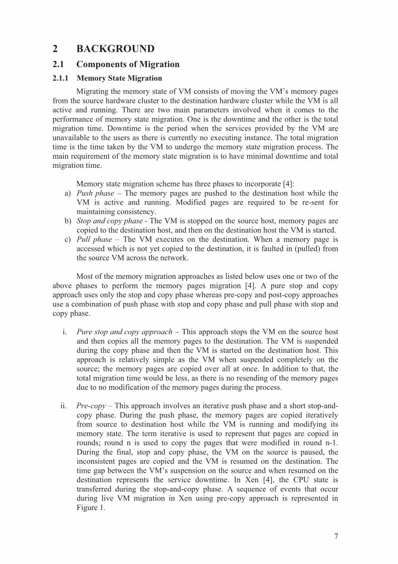
ii. Pre-copy – This approach involves an iterative push phase and a short stop-and-
copy phase. During the push phase, the memory pages are copied iteratively from source to destination host while the VM is running and modifying its memory state. The term iterative is used to represent that pages are copied in rounds; round n is used to copy the pages that were modified in round n-1. During the final, stop and copy phase, the VM on the source is paused, the inconsistent pages are copied and the VM is resumed on the destination. The time gap between the VM’s suspension on the source and when resumed on the destination represents the service downtime. In Xen [4], the CPU state is transferred during the stop-and-copy phase. A sequence of events that occur during live VM migration in Xen using pre-copy approach is represented in Figure 1.
Section 2 – BACKGROUND
8
Figure 1 - Xen Migration Time Line [4]
iii. Post-copy – In this approach, the VM on the source host is first suspended, the VM’s essential data structure is copied to destination and then the VM is resumed on the destination [4]. It can also be called as a short stop-and-copy phase. On demand the memory pages are then copied to the destination when the VM tries to access them. It produces the smallest downtime but it has the largest total migration time. Each page is transferred only once, and as a result this approach has lower network overhead compared to pre-copy approach.
2.1.2 Network State Migration
The Network states needs to be maintained to achieve a live migration, which is apparent to VM services and external clients. It can be achieved in a LAN quite easily. One way is sending a gratuitous ARP (Address Resolution Protocol) packet to the nodes in LAN and other way can be to send a RARP (Reverse ARP). Though, these ways cannot be implemented in a WAN as the VM’s IP address space would change.
A few of the current live migration implementations use a gratuitous ARP packet
such as the Xen facility while others such as VMware [18] use RARP to maintain the network connectivity during LAN based live migration. ARP tables of the ARP packets are updated by mapping the VM’s IP address to the advertised link-layer address [19].
Section 2 – BACKGROUND
9
Correspondingly, the LAN switches update their CAM (content addressable memory) tables when they receive ARP packets.
WAN-based VM migration has some key challenges to overcome. One of which
is maintaining the network connectivity and preserving the open connections during and after the migration. Data Centers interconnected over a WAN tend to use different IP address spaces. Therefore, a VM migrated between hosts over a WAN in different DC’s require a new IP address to be assigned by the network on the destination host. In addition, the old connections established with the old VM IP address space would be discarded.
A lot of research studies as mentioned in section 1.3 below shows proposed
different approaches to perform the live VM migration over WAN and maintain the networking connectivity as well. We found some to be very complicated and some to be scalable. We studied the solution based on VXLAN overlay networks and GRE tunneling between Cisco peers to overcome the drawbacks of WAN based live migration. Our main goal was to be able to maintain network connectivity after live migration of VMs over WAN resulting in minimal downtime and total migration time. VXLAN approach helps to create an isolated tunnel between the VMs source and destination end, which helps to send the VM traffic via the tunnel for secure and fast migration. Open vSwitch mobility between subnets feature in conjunction with VXLAN allows maintaining the network connectivity over WAN. GRE tunneling over Cisco Routers is the second approach we studied and implemented in our research to perform live migrations over the wide area network. A performance comparison is hence done using both the approaches and found some results. To the best of our knowledge this is the first time VXLAN and GRE tunneling over Cisco is used to achieve live VM migration across WAN.
2.1.3 Disk state migration Migration across a LAN generally transfers the memory, CPU and network states
when a shared storage is used [20]. Nonetheless, a shared storage might not be available always across a WAN based high latency low speed links. In such cases, the disk state also needs to be transferred with the VM states. In some cases, WAN’s may lead to undesirable disk read/write performance [1]. Current live VM migration implementations using the Xen’s migration facility are mostly designed for a LAN based environment. VMware for example has started its support for its storage migration vMotion solution [21].
The disk state migration can involve tens of gigabytes of memory to be migrated
and thus contributes to the largest overall migration time [1]. It comprises of transferring the VM’s local persistent state from source to destination host. The file system stored on the VM’s non-volatile local storage attributes to the local persistent state. The persistent state is not lost even if the system fails or its shutdown, unlike the run-time memory or CPU states.
Section 2 – BACKGROUND
10
2.2 Related Work 2.2.1 Disk State Migration
Luo et al. [22] discussed about a three-phase migration scheme as detailed above. The disk state is copied iteratively to the destination host, which is similar to the mechanism Xen uses to transfer its memory pages during the live migration. Modified blocks are tracked using the block bitmap during the pre-copy iterations and are resent to the destination in the consecutive iterations. The VM is suspended in the freeze and copy phase, the block bitmap is transferred and then the VM is being resumed on the destination side. The block bitmap illustrates the location of the blocks that were altered during the last iteration of the pre-copy phase. In the post-copy phase, the source host uses this block bitmap to push the altered blocks to the destination. The destination host on demand can pull the same block bitmap. If the VM is needed to be migrated back to the source host, only the altered blocks will need to be copied. The disk state migration time and the amount of data to be transferred is reduced using this scheme.
Akoush et al. [23] proposed an Activity Based Sector Synchronization (ABSS)
technique that would transfer VM disk images in an efficient manner. The modified sectors are identified and transferred that are likely to be modified at a later stage. This is useful in conserving the bandwidth and uses a statistically based synchronization algorithm to foresee the sectors that are likely to be altered.
Takahashi et al. [7] had suggested a disk state migration approach wherein a data
de-duplication technique is used to reduce the transfer time and the volume of data to be transferred. The VM is iteratively migrated between two fixed hosts in this scheme. A dirty block tracking mechanism was developed to track and record the disk page blocks updated when the VM is writing to it. Consider for example, a case where the VM is migrated between two hosts iteratively. The first disk state migration will take more time, as whole disk image needs to be transferred. In the subsequent migration though, it will take much shorter time, as only the updated pages would need to be transferred. This approach reduced the disk state migration time from 10 minutes to about 10 seconds and the volume of data to be transferred from 20 GB to several hundred megabytes.
Wood et al. [1] proposed a scheme named CloudNet wherein the Distributed
Replicated Block Device (DRBD) [24] is used for the disk state migration and DRBD asynchronous replication mode is used. A disk write is considered to be completed in the asynchronous mode when the disk write on the host is confirmed and the replication data is buffered for sending to the destination host [25]. The replication switches to the synchronous mode once the destination disk has been synchronized. A disk write is considered completed in the synchronous mode when the write has been confirmed by the local host and the destination host [25]. A block based Content Based Redundancy (CBR) [1] elimination technique is used in this scheme to save bandwidth when the disk and memory states are migrated.
Section 2 – BACKGROUND
11
2.2.2 Network State Migration Bradford et al. [5] proposed a combination of Dynamic DNS (Domain Name
Server) and IP tunneling to maintain the network state during WAN-based live migration. When the VM is about to be paused on the source host, an IP tunnel is setup-using iproute2 between the VM’s old IP address on the source host and its new IP address on the destination. Iproute2 is a set of utilities for networking and traffic control in Linux [26]. When the migration is completed, the DNS entry for the VM is updated with the new IP address so that new connections to the VM can avoid using the IP tunnel. This approach requires the VM to use two IP address at the same time, i.e., the VM is involved in this scheme. Furthermore, the source host has to keep forwarding packets belonging to VM’s old connections. As a result, the source host has to remain available until all VM’s old connections are closed. This can be problematic if, for example, the source host needs to be maintained or it should be turned off for power saving.
Travostino et al. [27] proposed a seamless VM migration scheme across
metropolitan area network (MAN) or WAN. In this scheme, clients that wish to communicate with the VM are required to setup an IP tunnel with VM’s host. When the VM is migrated to a new host, these tunnels need to be re-established. VM Traffic Controller (VMTC) facilitates dynamic tunnel creation and allows the VM to retain its IP address after migration without being involved in the process. But it has two problems. First, clients that are not configured to setup tunnel with VM’s host will not benefit from this solution. Second, resources available for tunnel creation and management limit the number of clients that VM’s host can serve.
Harney et al. [28] took a radically new approach in which they used Mobile IPv6
(MIPv6) protocol to support migration of VMs across WANs. The scheme in [28] involves enabling the mipv6 module in the TCP/IP protocol stack of VMs. MIPv6 has two advantages. Firstly, since the VM retains its original IP address, DNS updates are not needed to locate services on the VM. Secondly, MIPv6 provides the ability to use route optimization that enhances propagation delay of packets to and from the VM. The main problem with this approach is that it requires the VM to have modified protocol stack.
The authors in [1] have proposed a prototype named CloudNet, a cloud-
computing platform that coordinates with the underlying network provider to create seamless connectivity between the enterprise and data center sites as well as support live WAN migration of virtual machines. It is based on a commercial router-based VPLS (Virtual Private LAN service) / layer-2 VPN (Virtual Private Network) implementation. To minimize the amount of data transferred and lower the total migration time and application-experienced downtime, CloudNet is highly optimized.
The authors in [17] have presented a PMIPv6 approach, a lightweight mobility
protocol to maintain the network connectivity during the VM migration across the WAN. The approach is transparent to the VM from the network point of view and hence there was no need to install any mobility related software on the VM. PMIPv6 handles node mobility without requiring any support from the moving nodes. The author’s experimental results from a laboratory testbed showed that PMIPv6 approach achieved VM migration with minimal downtime and without any loss of established TCP
Section 2 – BACKGROUND
12
connection. Moreover, the results also showed that the signaling overhead was insignificant compared to other traffic generated during the VM migration.
CloudNet uses Multi-Protocol Label Switching (MPLS) based VPNs to create
the abstraction of a private network and address space shared by multiple data centers. It makes the level of abstraction even greater by using VPLS that bridge multiple MPLS endpoints onto a single LAN segment. Further VPLS provides transparent, secure, and resource guaranteed layer-2 connectivity without requiring sophisticated network configuration by end users. The IP address space would typically be different when the VM moves between routers at different sites, thus making it difficult to update the network configurations to seamlessly transfer active network connections. CloudNet avoids this problem by virtualizing the network connectivity so that the VM appears to be on the same virtual LAN and this is achieved by using VPLS VPN technology. Reconfiguring the VPNs that CloudNet can take advantage of to provide this abstraction typically takes a long time because of manual (or nearly manual) provisioning and configuration. CloudNet explicitly recognizes the need to set up new VPN endpoints quickly, and exploits the capability of BGP route servers [29] to achieve this.
Overlay networks stretch a Layer 2 network and increase mobility of virtual
machines. VXLAN (Virtual eXtensible LAN) is one of Layer 2 overlay schemes over a Layer 3 network proposed in IETF [8]. Each overlay is termed a VXLAN segment and only VMs within the same VXLAN segment can communicate with each other. VXLAN segment is identified through a 24-bit segment ID, termed the VXLAN Network Identifier (VNI). VNI identifies the scope of the inner MAC frame originated by the individual VM. Thus, you could have overlapping MAC addresses across segments but never have traffic "cross over" since the traffic is isolated using the VNI.
VXLAN is an IP multicast application and it uses IP multicast to isolate network
traffic. Authors in [30] describe implementations of VXLAN controller, edge switch with VXLAN gateway and OpenFlow switch. VXLAN controller is a management layer of VXLAN and manages VTEPs. VXLAN controller configures a mapping between the VXLAN VNI and the IP multicast group. And it also configures VTEP to join the IP multicast group when the VM is moved to the VTEP. If we simply apply VXLAN to Layer 2 network, we encounter the dynamic group member joining/leaving problems, which are common multicast problems in IP Network. But, the authors were able to describe a management method of IP multicast in VXLAN overlay networks and were able to eliminate the periodical Join/Leave messages.
2.3 Overview of Xen The University of Cambridge Computer Laboratory developed the first version
of Xen. Xen is an open source hypervisor that would allow running multiple OSes simultaneously on the same hardware. It is a type-1 baremetal hypervisor, runs in a more privileged CPU state than other software on the system. Several OSes can be run in parallel and a single machine [10]. Xen is also responsible for memory management, interrupt handling and CPU scheduling of VMs [10].
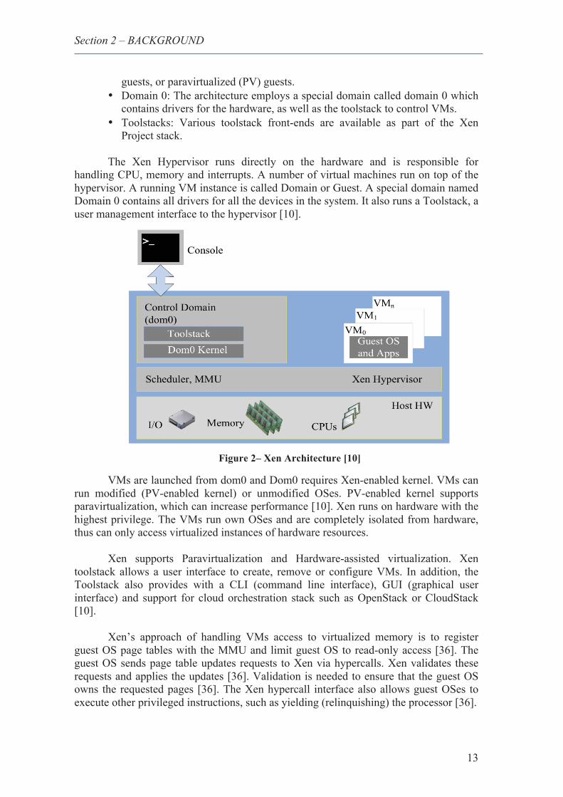
The key aspects of Xen architecture are as follows (as represented in Figure 2
below): • Guest types: The Xen Project hypervisor can run fully virtualized (HVM)
Section 2 – BACKGROUND
13
guests, or paravirtualized (PV) guests. • Domain 0: The architecture employs a special domain called domain 0 which
contains drivers for the hardware, as well as the toolstack to control VMs. • Toolstacks: Various toolstack front-ends are available as part of the Xen
Project stack.
The Xen Hypervisor runs directly on the hardware and is responsible for handling CPU, memory and interrupts. A number of virtual machines run on top of the hypervisor. A running VM instance is called Domain or Guest. A special domain named Domain 0 contains all drivers for all the devices in the system. It also runs a Toolstack, a user management interface to the hypervisor [10].
Figure 2– Xen Architecture [10]
VMs are launched from dom0 and Dom0 requires Xen-enabled kernel. VMs can run modified (PV-enabled kernel) or unmodified OSes. PV-enabled kernel supports paravirtualization, which can increase performance [10]. Xen runs on hardware with the highest privilege. The VMs run own OSes and are completely isolated from hardware, thus can only access virtualized instances of hardware resources.
Xen supports Paravirtualization and Hardware-assisted virtualization. Xen
toolstack allows a user interface to create, remove or configure VMs. In addition, the Toolstack also provides with a CLI (command line interface), GUI (graphical user interface) and support for cloud orchestration stack such as OpenStack or CloudStack [10].
Xen’s approach of handling VMs access to virtualized memory is to register
guest OS page tables with the MMU and limit guest OS to read-only access [36]. The guest OS sends page table updates requests to Xen via hypercalls. Xen validates these requests and applies the updates [36]. Validation is needed to ensure that the guest OS owns the requested pages [36]. The Xen hypercall interface also allows guest OSes to execute other privileged instructions, such as yielding (relinquishing) the processor [36].
Section 2 – BACKGROUND
14
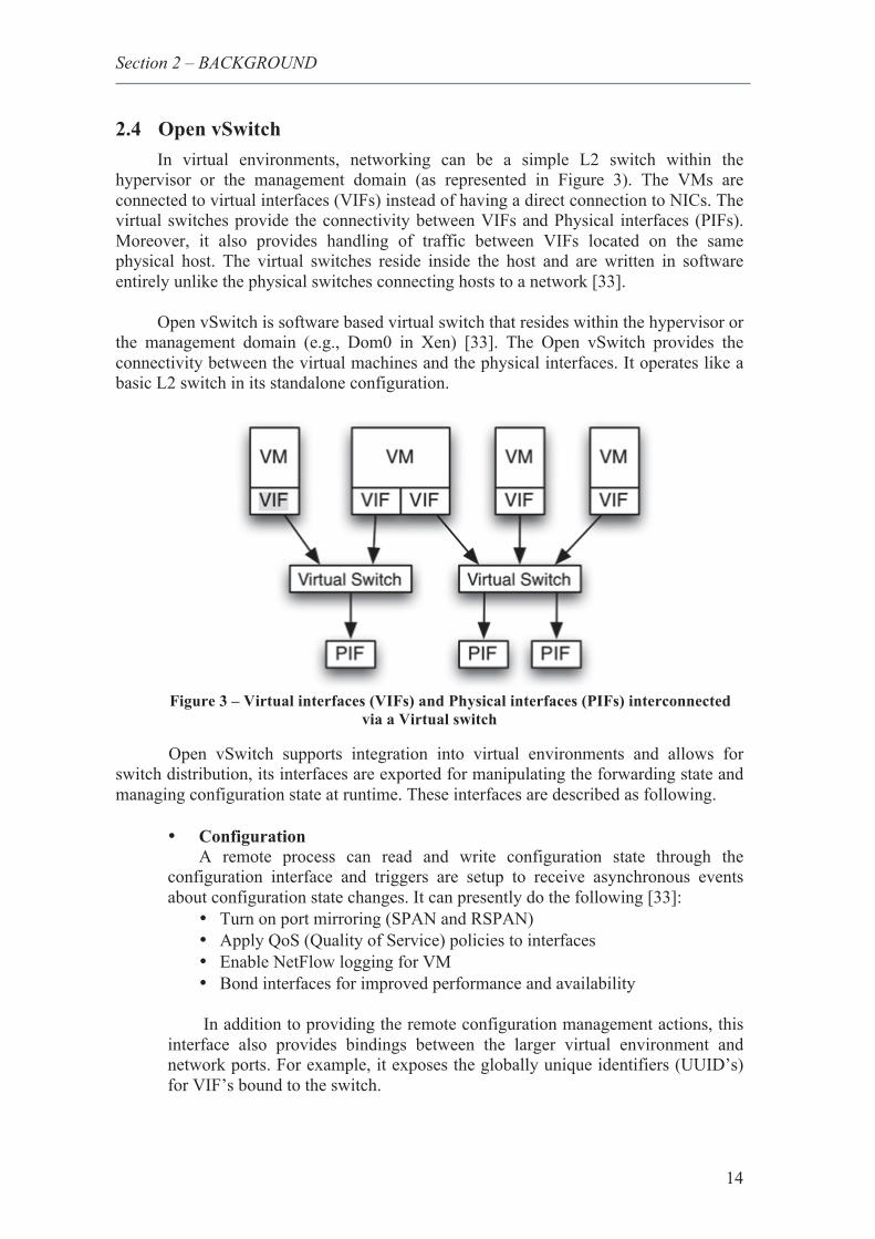
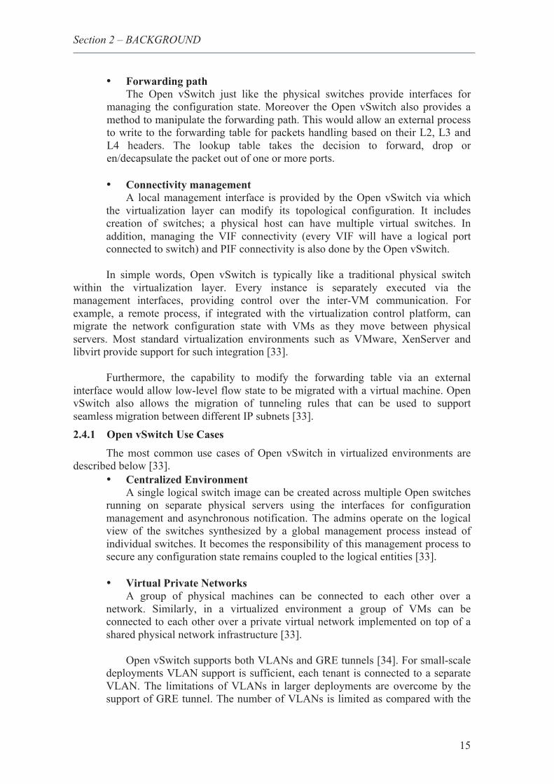
2.4 Open vSwitch In virtual environments, networking can be a simple L2 switch within the
hypervisor or the management domain (as represented in Figure 3). The VMs are connected to virtual interfaces (VIFs) instead of having a direct connection to NICs. The virtual switches provide the connectivity between VIFs and Physical interfaces (PIFs). Moreover, it also provides handling of traffic between VIFs located on the same physical host. The virtual switches reside inside the host and are written in software entirely unlike the physical switches connecting hosts to a network [33].
Open vSwitch is software based virtual switch that resides within the hypervisor or
the management domain (e.g., Dom0 in Xen) [33]. The Open vSwitch provides the connectivity between the virtual machines and the physical interfaces. It operates like a basic L2 switch in its standalone configuration.
Figure 3 – Virtual interfaces (VIFs) and Physical interfaces (PIFs) interconnected
via a Virtual switch
Open vSwitch supports integration into virtual environments and allows for switch distribution, its interfaces are exported for manipulating the forwarding state and managing configuration state at runtime. These interfaces are described as following.
• Configuration
A remote process can read and write configuration state through the configuration interface and triggers are setup to receive asynchronous events about configuration state changes. It can presently do the following [33]:
• Turn on port mirroring (SPAN and RSPAN) • Apply QoS (Quality of Service) policies to interfaces • Enable NetFlow logging for VM • Bond interfaces for improved performance and availability
In addition to providing the remote configuration management actions, this
interface also provides bindings between the larger virtual environment and network ports. For example, it exposes the globally unique identifiers (UUID’s) for VIF’s bound to the switch.
Section 2 – BACKGROUND
15
• Forwarding path The Open vSwitch just like the physical switches provide interfaces for
managing the configuration state. Moreover the Open vSwitch also provides a method to manipulate the forwarding path. This would allow an external process to write to the forwarding table for packets handling based on their L2, L3 and L4 headers. The lookup table takes the decision to forward, drop or en/decapsulate the packet out of one or more ports.
• Connectivity management
A local management interface is provided by the Open vSwitch via which the virtualization layer can modify its topological configuration. It includes creation of switches; a physical host can have multiple virtual switches. In addition, managing the VIF connectivity (every VIF will have a logical port connected to switch) and PIF connectivity is also done by the Open vSwitch.
In simple words, Open vSwitch is typically like a traditional physical switch
within the virtualization layer. Every instance is separately executed via the management interfaces, providing control over the inter-VM communication. For example, a remote process, if integrated with the virtualization control platform, can migrate the network configuration state with VMs as they move between physical servers. Most standard virtualization environments such as VMware, XenServer and libvirt provide support for such integration [33].
Furthermore, the capability to modify the forwarding table via an external
interface would allow low-level flow state to be migrated with a virtual machine. Open vSwitch also allows the migration of tunneling rules that can be used to support seamless migration between different IP subnets [33]. 2.4.1 Open vSwitch Use Cases
The most common use cases of Open vSwitch in virtualized environments are described below [33].
• Centralized Environment A single logical switch image can be created across multiple Open switches
running on separate physical servers using the interfaces for configuration management and asynchronous notification. The admins operate on the logical view of the switches synthesized by a global management process instead of individual switches. It becomes the responsibility of this management process to secure any configuration state remains coupled to the logical entities [33].
• Virtual Private Networks
A group of physical machines can be connected to each other over a network. Similarly, in a virtualized environment a group of VMs can be connected to each other over a private virtual network implemented on top of a shared physical network infrastructure [33].
Open vSwitch supports both VLANs and GRE tunnels [34]. For small-scale
deployments VLAN support is sufficient, each tenant is connected to a separate VLAN. The limitations of VLANs in larger deployments are overcome by the support of GRE tunnel. The number of VLANs is limited as compared with the
Section 2 – BACKGROUND
16
size of virtual environments. In GRE tunnel, encapsulation of an Ethernet frame inside an IP datagram is done. For Open vSwitch, the GRE tunnel is used to route traffic from one subnet to another. If the communicating VMs are on a single host, the VPN would exist in a single Open vSwitch; If the VMs are all on the same subnet, the management process will make use of VLANs to setup the private network and finally if the VMs span multiple subnets, it can use GRE tunnels.
• Mobility between IP subnets
Today’s commercial virtualization platforms have a well-known limitation that migration must happen within a single IP subnet. The inability to maintain the transport sessions over changes in the endpoint address is the main reason behind such limitation. Migration between different subnets is needed for a lot of reasons. For example, single L2 domains have scalability limits; operators need to segment their networks, imposing artificial limits on mobility.
Out of many ways to accomplish this using Open vSwitch and a global
management process, the most direct way is to use a model similar to Mobile IP wherein an Open vSwitch would receive all the packets for a given VM and then forward the packets using tunneling to the correct location.
The Open vSwitch’s primary environment is a Linux-based virtualization
platform. Integration with them requires the Open vSwitch to emulate the interfaces of VDE (Virtual Distributed Ethernet) [35] and the Linux bridging code. The VDE and Linux bridging code are both commonly used in virtual deployments. Therefore, the Xen, XenServer and KVM can use Open vSwitches instead of virtual switches as a replacement. Due to Open vSwitch’s exporting of ioctl, sysfs and proc filesystem interfaces, most of the tools and utilities can be run unmodified against it [33].
17
3 PURPOSE 3.1 Problem Statement
In the present stage, VMM platforms such as Xen and VMware support live migration in LAN. The live migration functionality relies on the assumption that hypervisors are co-located in the same broadcast domain, that they are part of the same IP address space, and that a shared storage system is available. In general, these assumptions do not hold when hypervisors are interconnected over a WAN. These limitations are typically overcome by virtualizing the network functionality, such as to “trick” the hypervisors into believing that the migration assumptions are fulfilled.
For a successful and efficient live VM migration across WAN, several
challenges need to be addressed [1]:
1. Minimize downtime – The time period when a system is down or not responding is termed as downtime. The downtime should be minimized, so that there is no disruption in the services the clients are accessing.
2. Minimize network reconfigurations – Migration over LAN can be done transparently, as the VM can retain its IP address after migration. But over WAN the problem arises of the IP address being changed and doing so transparently, is a major challenge. The network connections established with VM’s old IP address would be dropped.
3. Optimized Routing – The routing should be optimized for lower latency using the shortest hops to the destination. In order to reduce the packet propagation delay, it is desirable that the traffic between clients and VM should follow an optimum path. Long propagation delays would result in bad user experience due to slow responsiveness of services.
4. Handle WAN links – WAN links interconnecting data centers are bandwidth constrained and inter-data center latencies are higher than in a LAN. Consequently, WAN migration techniques must be designed to operate efficiently over low bandwidth links. It may not be possible to dedicate hundreds of MBps (Mega Bytes per second) of bandwidth for a single VM transfer even if WAN links were provisioned with high bandwidth.
5. Support for IPv4, IPv6 or dual stack VM’s – It is necessary that a WAN-based VM migration solution is designed to support IPv4, IPv6 and dual stack VM’s.
6. Migration is Transparent to Client – The clients should not be involved in the VM migration process in maintaining open connections. The VM migration over WAN should not rely on the configuration or any software installed on the VM.
VXLAN is typically deployed in data centers on virtualized hosts, which may be spread across multiple racks. The individual racks may be parts of a different Layer 3 network or they could be in a single Layer 2 network. It encapsulates data packets, establishes connection between end points (VTEP), VTEP connection via existing IP infrastructure. It provides 24-bit network identifier (VNI (VXLAN network identifier) - defines VXLAN segment) and VM to VM communication only within the same VXLAN segment. Further, VMs can use the same MAC/IP addresses in different VXLAN segments and VM is unaware of the encapsulation.
Section 3 – PURPOSE
18
3.2 Research question 1. What previous efforts have been made to support live VM migration across
WAN? 2. How can a GRE tunnel-based approach over Cisco routers be used to maintain
network connectivity during live migration of VMs over WAN? 3. How can a VXLAN-based approach be used to maintain network connectivity
during live migration of VMs over WAN? 4. What metrics can be used to measure the effectiveness of our solutions? 5. Is a GRE tunnel-based approach more efficient than the VXLAN-approach in
maintaining network connectivity during live migration of VMs over WAN?
3.3 Goals Achieved The goal of our thesis work is to investigate the performance of VXLAN and
GRE tunnel-based approaches for VM live migration over the WAN, with emphasis on network state migration. We have used Xen, an open source hypervisor to support the live migration of virtual machines. With the VXLAN and GRE tunnel based approaches used to maintain the network connectivity, the following goals have been achieved:
• Maintained the network connectivity while the VM is migrating over the
WAN. • Achieved minimal downtime and ensured service continuity during live VM
migration. • Preserved the VM’s IP address after migration. • Calculated the downtime and total migration time involved during the
migration process. • Developed a Client Server program to measure the downtime and total
migration time. • Examined the survivability of Transmission Control Protocol (TCP)
connections during and after the migration. • Compared our VXLAN [8] approach of VM migration with the GRE tunnel
based approach and make recommendation which one to choose for specific scenarios.
19
4 APPROACHES TO ACHIEVE LIVE VM MIGRATION In this Chapter, we have described in detail about the approaches we have used
to perform the live VM migration over the cloud and maintain the network connectivity while the VM migrates. A brief overview of Xen hypervisor is also discussed.
We have considered the VXLAN and GRE tunnel over Cisco approach to establish and maintain the network connectivity while using Xen [10] as a virtualization platform to implement and test our solution. VXLAN and Cisco GRE tunneling can also be implemented using other virtualization platforms providing live migration facilities. Xen handles the migration of VM’s memory and CPU states while the approaches used allowed maintaining the network connectivity. The disk state of the VM is assumed to exist on a shared storage medium.
We have focused to work on the open source platforms. Xen being a powerful open source hypervisor is considered that provided us with a suitable platform to implement and test our solution. We have avoided Kernel-based Virtual Machine (KVM), which is another powerful hypervisor alternative, because it requires the VM hosts to support hardware-assisted virtualization. The hosts we used in our setup did not have support for full hardware virtualization.
4.1 VXLAN The Data centers need to host multiple tenants, each with their own isolated
network domain. The VM’s are grouped according to their specific Virtual LAN (VLAN, might need thousands of VLAN’s to partition the traffic the VM belongs to). The current VLAN limit is 4096, which is inadequate in such situations [31].
In addition to that, while virtualization has reduced the cost and time required to
deploy a new application from weeks to minutes, reducing the costs from thousands of dollars to a few hundred, reconfiguring the network for a new or migrated virtual workload can take a week and cost thousands of dollars. Scaling an existing network technology requires possible solutions to enable VM communication and its migration across Layer 3 boundaries without impacting the network connectivity while ensuring the isolation for hundred of thousands of logical network segments and maintaining existing VM addresses and Media Access Control (MAC) addresses. VXLAN, an IETF proposed standard by VMware, Emulex, Cisco and other leading organizations address these challenges [9].
VXLAN is used in virtualized data centers to accommodate multiple tenants and
address the need for overlay networks. One of the important requirement while considering a Layer 2 infrastructure for a virtualized environment is having the Layer 2 network scale across the entire data center or even between data centers for efficient allocation of compute, network and storage resources [31]. The VM’s MAC traffic is carried in an encapsulated format over a logical tunnel by the overlay network.
VXLAN is intended to address the following issues [31]. The focus is on the
networking infrastructure within the data center and the issues related to them.
A. Limitations imposed by Spanning Tree & VLAN Ranges The Layer 2 networks use the IEEE 802.1D Spanning Tree Protocol to avoid
loops in the network due to duplicate paths. This becomes a problem for the data
Section 4 – APPROCHES TO ACHIEVE LIVE VM MIGRATION
20
center operators with layer 2 networks, since with STP they are paying for more ports and links they can actually use.
One of the key characteristics of layer 2 networks is their use of Virtual LAN’s to provide broadcast isolation. A 12-bit VLAN ID is used in data frames to divide a larger Layer 2 networks into multiple broadcast domains. This serves well for data centers, which require fewer than 4096 VLAN’s. But this upper limit is seeing pressure. B. Multitenant Environments
For layer 2 networks, VLAN’s are often used to segregate traffic, so that a tenant can be identified by its own VLAN ID. The 4096 VLAN limit becomes inadequate when it comes to providing service to a large number of tenants. Further, this issue exacerbates when there is often a need for multiple VLAN’s per tenant.
VXLAN addresses the above requirements of the layer 2 and layer 3 data center network infrastructure in the presence of VM’s in a multi-tenant environment. VXLAN also termed as a tunneling protocol, is a Layer 2 overlay scheme over a Layer 3 network. Each overlay is termed as VXLAN segment and VM’s only within the same VXLAN segment can communicate with each other. Each segment is identified by a 24-bit segment ID (termed as VXLAN Network Identifier (VNI)). This can allow up to 16M VXLAN segments to exist within the same administrative domain [31].
The scope of the inner MAC frame originated by the individual VM is identified
by the VNI. There could arise a problem of overlapping MAC address across the segments but there would never be traffic cross over since the traffic is isolated by the VNI. The inner MAC frame originated by the VM is encapsulated in an outer header, which is termed as VNI. VXLAN could be termed as a tunneling scheme due to such encapsulation to overlay layer 2 networks on top of layer 2 networks. VTEP (VXLAN tunnel end point) is the end point of the tunnel and is located within the hypervisor, which hosts the VM on the server. The VNI and VXLAN tunnel/outer header encapsulation are not known to the VM, it is known to VTEP only.
4.1.1 Unicast VM to VM communication
VM to VM communication from one host to another is taken place by sending in a MAC frame destined to the target as normal. The VM is unaware of the VXLAN. The VTEP on the host firstly looks for the VNI to which the VM is related. Secondly, it finds out if the destination MAC address is on the same segment. Thirdly, it checks if there is a mapping between the destinations MAC address to the remote VTEP. If a mapping is found then an outer header consisting of an outer MAC, outer IP header and VXLAN header is prepended to the original MAC frame. The encapsulated packet is forwarded to the remote VTEP. Upon reception, the validity of the VNI of the remote VTEP is verified and checks for a VM on that VNI using a MAC address that would match the inner destination MAC address.
Section 4 – APPROCHES TO ACHIEVE LIVE VM MIGRATION
21
If a match is found, the packet is stripped of its headers and forwarded to the destination VM. The destination VM does not know about the VNI or about the frame that was transported with a VXLAN encapsulation. In addition to that, the Inner Source MAC to outer Source IP address mapping is done by the VTEP. The mapping is stored in a table and there is no need for an unknown destination flooding of the response packet when the destination VM sends a response packet.
4.1.2 Broadcast Communication and mapping to multicast Considering a case when the VM on the source wants to communicate with the
VM on the destination VM using IP, the VM sends out an ARP broadcast frame, assuming that they are both on the same subnet. This frame would be sent out across all the switches carrying the VLAN using MAC broadcast in a non-VXLAN environment.
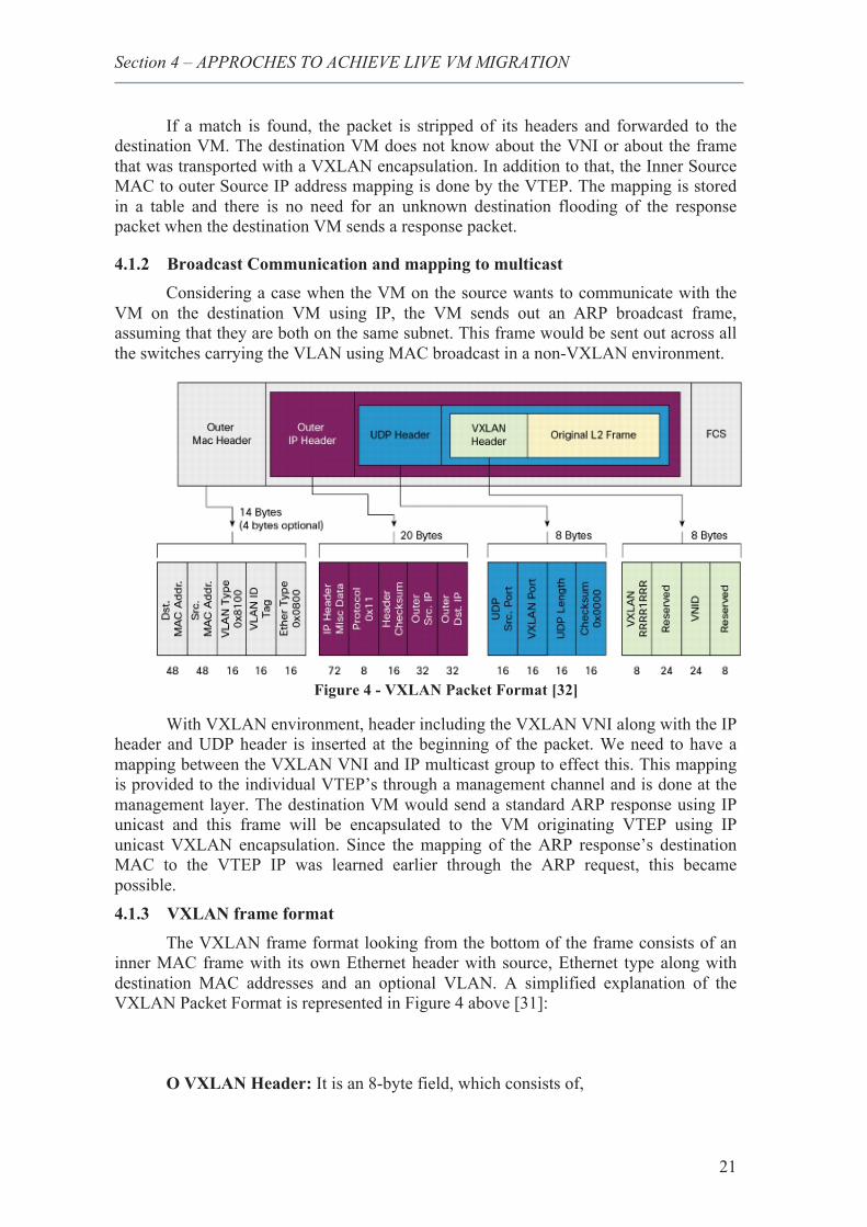
Figure 4 - VXLAN Packet Format [32]
With VXLAN environment, header including the VXLAN VNI along with the IP header and UDP header is inserted at the beginning of the packet. We need to have a mapping between the VXLAN VNI and IP multicast group to effect this. This mapping is provided to the individual VTEP’s through a management channel and is done at the management layer. The destination VM would send a standard ARP response using IP unicast and this frame will be encapsulated to the VM originating VTEP using IP unicast VXLAN encapsulation. Since the mapping of the ARP response’s destination MAC to the VTEP IP was learned earlier through the ARP request, this became possible. 4.1.3 VXLAN frame format
The VXLAN frame format looking from the bottom of the frame consists of an inner MAC frame with its own Ethernet header with source, Ethernet type along with destination MAC addresses and an optional VLAN. A simplified explanation of the VXLAN Packet Format is represented in Figure 4 above [31]:
O VXLAN Header: It is an 8-byte field, which consists of,
Section 4 – APPROCHES TO ACHIEVE LIVE VM MIGRATION
22
• Flags (8 bits) – The I flag MUST be set to 1 for a valid VXLAN ID (VNI). The 7 left out bits are reserved fields.
• VXLAN Segment ID/VNI – It is a 24-bit value used to allocate the individual VXLAN overlay network on which the communicating VM’s are situated.
• O Reserved fields (24 bits and 8 bits) – It MUST be set to zero on transmit and ignore on receive.
O Outer UDP Header: It is the outer UDP header where the source port is the VTEP and the destination port is the well-known UDP port. The value of 4789 is assigned by IANA for the VXLAN UDP port and is used as a default value for the destination UDP port. O Outer IP Header: It is the outer IP header with the source IP address being the IP address of the VTEP where the VM is running. The destination IP address could be a unicast or multicast IP address.
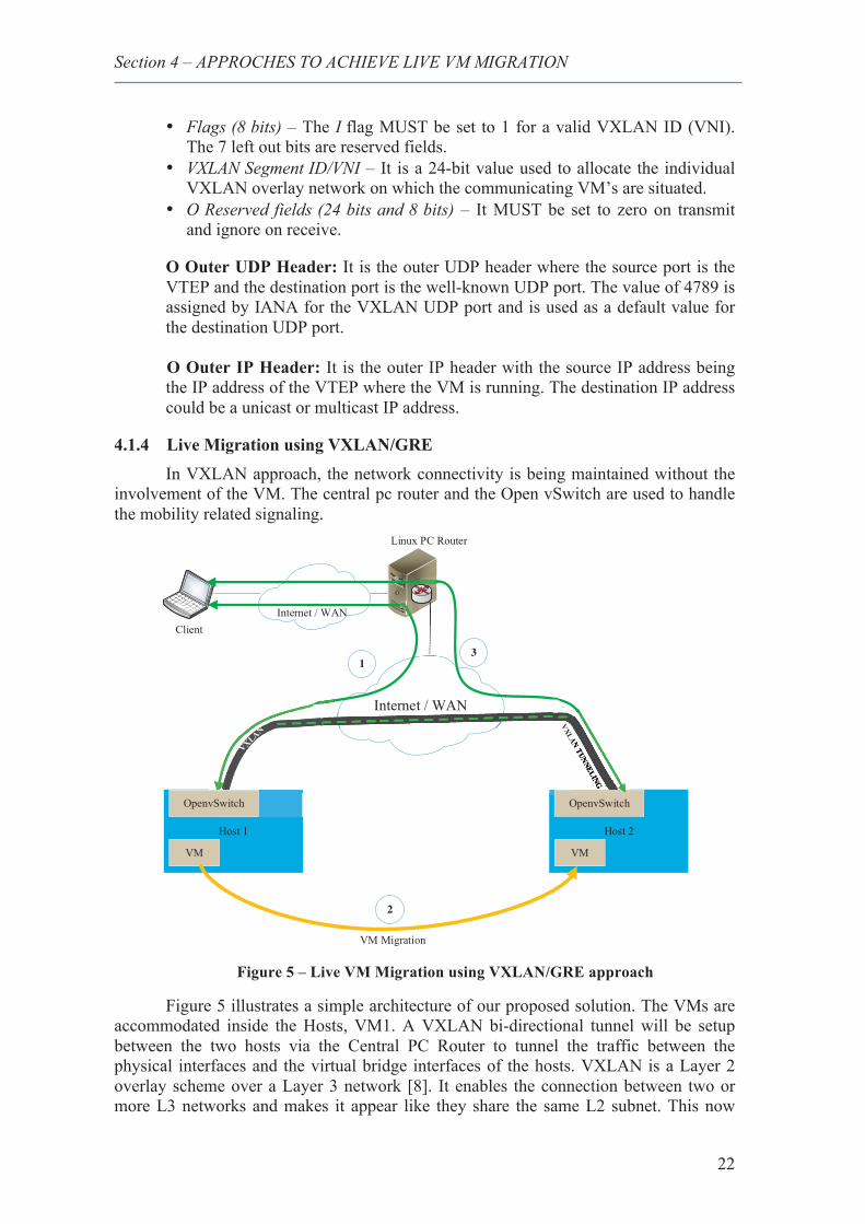
4.1.4 Live Migration using VXLAN/GRE
In VXLAN approach, the network connectivity is being maintained without the involvement of the VM. The central pc router and the Open vSwitch are used to handle the mobility related signaling.
Figure 5 – Live VM Migration using VXLAN/GRE approach
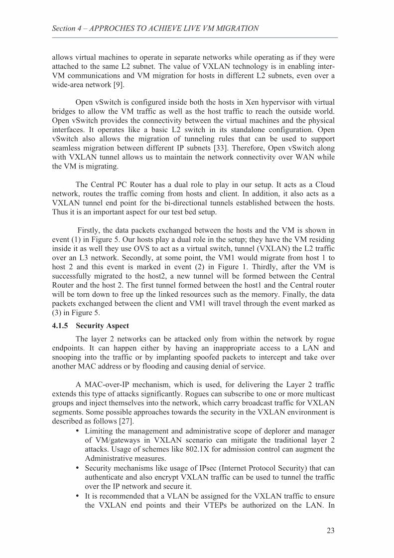
Figure 5 illustrates a simple architecture of our proposed solution. The VMs are accommodated inside the Hosts, VM1. A VXLAN bi-directional tunnel will be setup between the two hosts via the Central PC Router to tunnel the traffic between the physical interfaces and the virtual bridge interfaces of the hosts. VXLAN is a Layer 2 overlay scheme over a Layer 3 network [8]. It enables the connection between two or more L3 networks and makes it appear like they share the same L2 subnet. This now
ClientInternet / WAN
Internet / WAN
Host 1 Host 2
VM VM
Linux PC Router
VM Migration
13
2
OpenvSwitch OpenvSwitch
Section 4 – APPROCHES TO ACHIEVE LIVE VM MIGRATION
23
allows virtual machines to operate in separate networks while operating as if they were attached to the same L2 subnet. The value of VXLAN technology is in enabling inter-VM communications and VM migration for hosts in different L2 subnets, even over a wide-area network [9].
Open vSwitch is configured inside both the hosts in Xen hypervisor with virtual
bridges to allow the VM traffic as well as the host traffic to reach the outside world. Open vSwitch provides the connectivity between the virtual machines and the physical interfaces. It operates like a basic L2 switch in its standalone configuration. Open vSwitch also allows the migration of tunneling rules that can be used to support seamless migration between different IP subnets [33]. Therefore, Open vSwitch along with VXLAN tunnel allows us to maintain the network connectivity over WAN while the VM is migrating.
The Central PC Router has a dual role to play in our setup. It acts as a Cloud
network, routes the traffic coming from hosts and client. In addition, it also acts as a VXLAN tunnel end point for the bi-directional tunnels established between the hosts. Thus it is an important aspect for our test bed setup.
Firstly, the data packets exchanged between the hosts and the VM is shown in
event (1) in Figure 5. Our hosts play a dual role in the setup; they have the VM residing inside it as well they use OVS to act as a virtual switch, tunnel (VXLAN) the L2 traffic over an L3 network. Secondly, at some point, the VM1 would migrate from host 1 to host 2 and this event is marked in event (2) in Figure 1. Thirdly, after the VM is successfully migrated to the host2, a new tunnel will be formed between the Central Router and the host 2. The first tunnel formed between the host1 and the Central router will be torn down to free up the linked resources such as the memory. Finally, the data packets exchanged between the client and VM1 will travel through the event marked as (3) in Figure 5. 4.1.5 Security Aspect
The layer 2 networks can be attacked only from within the network by rogue endpoints. It can happen either by having an inappropriate access to a LAN and snooping into the traffic or by implanting spoofed packets to intercept and take over another MAC address or by flooding and causing denial of service.
A MAC-over-IP mechanism, which is used, for delivering the Layer 2 traffic
extends this type of attacks significantly. Rogues can subscribe to one or more multicast groups and inject themselves into the network, which carry broadcast traffic for VXLAN segments. Some possible approaches towards the security in the VXLAN environment is described as follows [27].
• Limiting the management and administrative scope of deplorer and manager of VM/gateways in VXLAN scenario can mitigate the traditional layer 2 attacks. Usage of schemes like 802.1X for admission control can augment the Administrative measures.
• Security mechanisms like usage of IPsec (Internet Protocol Security) that can authenticate and also encrypt VXLAN traffic can be used to tunnel the traffic over the IP network and secure it.
• It is recommended that a VLAN be assigned for the VXLAN traffic to ensure the VXLAN end points and their VTEPs be authorized on the LAN. In
Section 4 – APPROCHES TO ACHIEVE LIVE VM MIGRATION
24
addition, the VTEPs send the VXLAN traffic over the LAN to provide a sense of security.
4.1.6 VXLAN Use Cases
• Server racks Capacity expansion A single rack constituting of multiple host servers all residing in a common
cluster or pod (termed as Virtual data center) provides a small-virtualized environment for a single tenant. Each rack may constitute an L2 subnet, while multiple host server racks in a cluster would likely be assigned their own L3 network [9].
The demand for expansion of additional computing resource by the tenant
might require more number of servers or the VMs on a different rack, within a different L2 subnet or on a different host cluster, in a different L3 network. The new VMs need to communicate with the applications VM on the primary rack or cluster [9].
• VM Migration to another cluster
A need for migration of VM(s) to another server cluster (inter-host workload mobility) arises to optimize the usage of the underlying server hardware resources [9].
There may be two scenarios that might exist, a) The underutilized hosts are migrated to consolidate the more fully
utilized hosts to reduce the energy needs. b) The underutilized hosts are shutdown to consolidate the more fully
utilized hosts to reduce the energy needs. c) Make the older hosts inactive and bring up the workloads on the newer
hosts. 4.1.7 VM-VM Communication
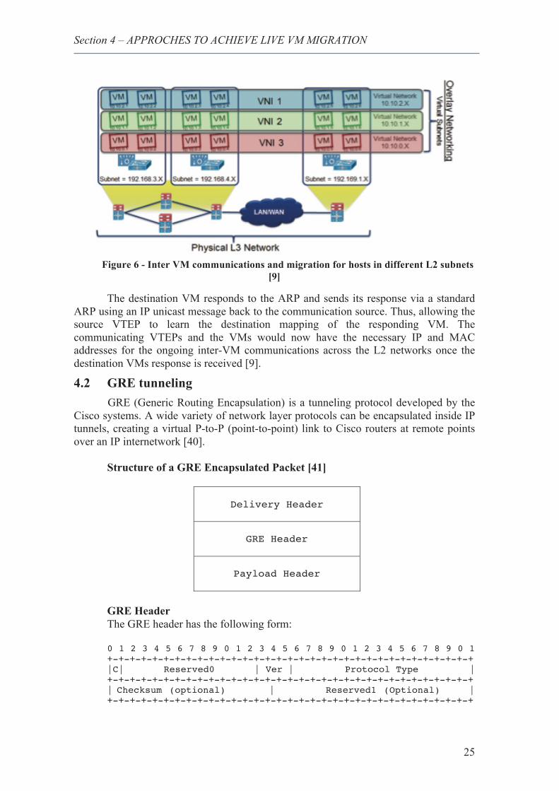
The importance of the VXLAN technology lies in enabling the VM-VM communications and migration of hosts for different L2 subnets. An elementary explanation of the process is illustrated in Figure 6 below [9].
The Xen hosts would act as the VTEPs for our setup and the VTEP’s would be
responsible for setting up the VXLAN header needed to establish the 24-bit VNI. In addition, VTEP also implements the UDP and outer Ethernet encapsulations which are needed to communicate across the L3 network. The VM here is unaware of this VNI tag [9].
The communicating source VM initially sends a broadcast ARP message. The source host, which acts as a VTEP, will encapsulate the packet and send as a broadcast packet to the IP multicast group related to the VXLAN segment (VNI) to which the communicating VM’s belong. The VTEP’s, which are not participating in the VM communication, would learn the inner MAC address of the source VM and the Outer IP address of its related VTEP from this packet [9].
Section 4 – APPROCHES TO ACHIEVE LIVE VM MIGRATION
25
Figure 6 - Inter VM communications and migration for hosts in different L2 subnets
[9]
The destination VM responds to the ARP and sends its response via a standard ARP using an IP unicast message back to the communication source. Thus, allowing the source VTEP to learn the destination mapping of the responding VM. The communicating VTEPs and the VMs would now have the necessary IP and MAC addresses for the ongoing inter-VM communications across the L2 networks once the destination VMs response is received [9].
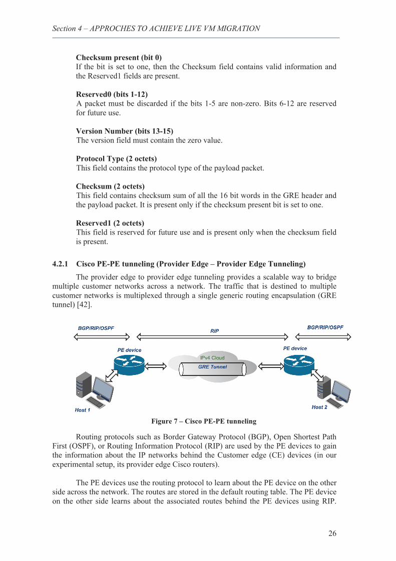
4.2 GRE tunneling GRE (Generic Routing Encapsulation) is a tunneling protocol developed by the
Cisco systems. A wide variety of network layer protocols can be encapsulated inside IP tunnels, creating a virtual P-to-P (point-to-point) link to Cisco routers at remote points over an IP internetwork [40].
Structure of a GRE Encapsulated Packet [41]
Delivery Header
GRE Header
Payload Header
GRE Header The GRE header has the following form:
0 1 2 3 4 5 6 7 8 9 0 1 2 3 4 5 6 7 8 9 0 1 2 3 4 5 6 7 8 9 0 1 +-+-+-+-+-+-+-+-+-+-+-+-+-+-+-+-+-+-+-+-+-+-+-+-+-+-+-+-+-+-+-+-+ |C| Reserved0 | Ver | Protocol Type | +-+-+-+-+-+-+-+-+-+-+-+-+-+-+-+-+-+-+-+-+-+-+-+-+-+-+-+-+-+-+-+-+ | Checksum (optional) | Reserved1 (Optional) | +-+-+-+-+-+-+-+-+-+-+-+-+-+-+-+-+-+-+-+-+-+-+-+-+-+-+-+-+-+-+-+-+
Section 4 – APPROCHES TO ACHIEVE LIVE VM MIGRATION
26
Checksum present (bit 0) If the bit is set to one, then the Checksum field contains valid information and the Reserved1 fields are present. Reserved0 (bits 1-12) A packet must be discarded if the bits 1-5 are non-zero. Bits 6-12 are reserved for future use. Version Number (bits 13-15) The version field must contain the zero value. Protocol Type (2 octets) This field contains the protocol type of the payload packet. Checksum (2 octets) This field contains checksum sum of all the 16 bit words in the GRE header and the payload packet. It is present only if the checksum present bit is set to one. Reserved1 (2 octets) This field is reserved for future use and is present only when the checksum field is present.
4.2.1 Cisco PE-PE tunneling (Provider Edge – Provider Edge Tunneling) The provider edge to provider edge tunneling provides a scalable way to bridge
multiple customer networks across a network. The traffic that is destined to multiple customer networks is multiplexed through a single generic routing encapsulation (GRE tunnel) [42].
Figure 7 – Cisco PE-PE tunneling
Routing protocols such as Border Gateway Protocol (BGP), Open Shortest Path First (OSPF), or Routing Information Protocol (RIP) are used by the PE devices to gain the information about the IP networks behind the Customer edge (CE) devices (in our experimental setup, its provider edge Cisco routers).
The PE devices use the routing protocol to learn about the PE device on the other
side across the network. The routes are stored in the default routing table. The PE device on the other side learns about the associated routes behind the PE devices using RIP.
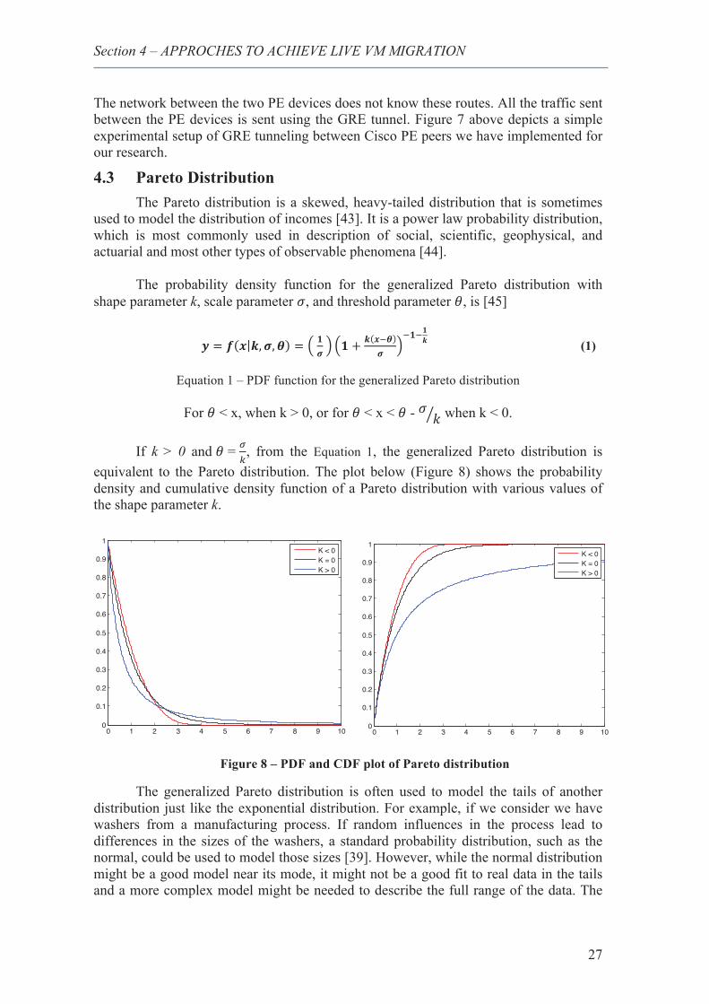
Section 4 – APPROCHES TO ACHIEVE LIVE VM MIGRATION
27
The network between the two PE devices does not know these routes. All the traffic sent between the PE devices is sent using the GRE tunnel. Figure 7 above depicts a simple experimental setup of GRE tunneling between Cisco PE peers we have implemented for our research.
4.3 Pareto Distribution The Pareto distribution is a skewed, heavy-tailed distribution that is sometimes
used to model the distribution of incomes [43]. It is a power law probability distribution, which is most commonly used in description of social, scientific, geophysical, and actuarial and most other types of observable phenomena [44].
The probability density function for the generalized Pareto distribution with
shape parameter k, scale parameter , and threshold parameter , is [45]
(1)
Equation 1 – PDF function for the generalized Pareto distribution
For < x, when k > 0, or for < x < - when k < 0.
If k > 0 and = , from the Equation 1, the generalized Pareto distribution is equivalent to the Pareto distribution. The plot below (Figure 8) shows the probability density and cumulative density function of a Pareto distribution with various values of the shape parameter k.
Figure 8 – PDF and CDF plot of Pareto distribution
The generalized Pareto distribution is often used to model the tails of another distribution just like the exponential distribution. For example, if we consider we have washers from a manufacturing process. If random influences in the process lead to differences in the sizes of the washers, a standard probability distribution, such as the normal, could be used to model those sizes [39]. However, while the normal distribution might be a good model near its mode, it might not be a good fit to real data in the tails and a more complex model might be needed to describe the full range of the data. The
0 1 2 3 4 5 6 7 8 9 100
0.1
0.2
0.3
0.4
0.5
0.6
0.7
0.8
0.9
1
K < 0K = 0K > 0
0 1 2 3 4 5 6 7 8 9 100
0.1
0.2
0.3
0.4
0.5
0.6
0.7
0.8
0.9
1
K < 0K = 0K > 0
Section 4 – APPROCHES TO ACHIEVE LIVE VM MIGRATION
28
generalized Pareto distribution can thus be used to provide a good fit to extremes of complicated data [39].
The Pareto distribution is used to model the effect of long-tails and heavy-tails.
We have considered using Pareto distribution for our experimental test bed instead of the default uniform distribution, the reason being the existence of long-tails in the distribution of session duration in wide area networks which is supported by empirical evidence from several studies [46,47,48].
4.4 Custom NetEm Distribution The NetEm is widely used to achieve emulated network environments in
networking research and can be used to evaluate new protocols and applications under controlled and repeatable conditions. It provides Network Emulation functionality for testing protocols by emulating the properties of a WAN. The current version can emulate variable delay, loss, duplication and reordering [39]. Netem allows creating custom distribution tables using the iproute2 source code to better approximate the round-trip-time variations in the network.
We have worked on creating custom distribution tables using the iproute2 source
code as a reference which is located at “/usr/lib/tc”. Our main aim was to emulate a WAN scenario by calculating the mean (mu) standard deviation (sigma) and correlation (rho) of the round-trip-time. We emulated the network between a server in Europe and our client PC in Sweden by running a ping between the two machines for a whole day. Later, using the inbuilt Linux tools supported by the iproute2, we were able to determine the metrics mu, sigma and rho. These metrics can be used in the Netem equation in place of delay, jitter and correlation to emulate a WAN scenario between a server in Europe and Sweden. But, the results being not so reliable to depict the emulation of the whole European region based on a single server round-trip-time data. We have not used it for our experimental testbed. The setup steps for creating own distribution are documented in the Appendix Section E.
.
29
5 Research Methodology In this Chapter, the methodology used for our research has been described.
Moreover, the reasons for choosing the method of study are explained. In addition, the experimental scenarios and the performance metrics used for evaluation are also discussed in detail in this chapter.
It requires that the solution be modeled correctly. Our research method can be
divided into three phases as follows:
Phase 1: In the first phase, we have done a thorough literature review on our research area
by reading various articles, journals and magazines. We have referred to several databases like IEEE explore, ACM Digital library, etc.
Phase 2: In this phase, we have setup a laboratory experimental testbed to evaluate our
approach of live migration across WAN which allowed us to evaluate our setup in a real-world environment. An experimental setup has a lot of advantages over simulation methods. Our focus of research was on testing the practicality of using the VXLAN and GRE tunneling approach for performing the live migration of virtual machine and to maintain the network connectivity over WAN. The behavior of the system under study is too complex to be captured by a simulation or mathematical model, thus a real time environmental setup was necessary. Our research is carried out on the basis of the previous work carried out by the researchers. To test the scalability of our solution, simulation can turn out to be a suitable method to virtually simulate a real time model.
Phase 3: In the final phase, we have analyzed the performance of using the two live
migration approaches namely, GRE tunneling and VXLAN based on the performance metrics.
5.1 Test bed Our laboratory testbed was setup to test the efficacy of the VXLAN approach
GRE tunneling approach in maintaining the network connectivity over the WAN during the VM migration. Xen, Open vSwitch and VXLAN/GRE tunnel actively work combinable to transfer the CPU, memory and network states of the VM from the source to the destination hosts. A shared storage medium is used to store the VMs disk state. The testbed was used to compare the performance of both the GRE tunneling/VXLAN approaches towards live VM migration.
Our testbed architecture is shown in Figure 9, it consists of five Linux based OS
systems. All the systems run on latest Ubuntu 14.04.1 LTS OSes with the latest kernel. The Xen 4.3 release will feature initial integration of Open vSwitch based networking. Conceptually this is similar to a bridged configuration but rather than placing each vif on a Linux bridge instead an Open vSwitch switch is used [38]. Thus, the hosts were installed with the latest Xen 4.4 hypervisor to provide full support for Open vSwitch and VXLAN tunneling protocol.
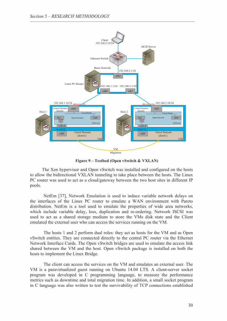
Section 5 – RESEARCH METHODOLOGY
30
Figure 9 – Testbed (Open vSwitch & VXLAN)
The Xen hypervisor and Open vSwitch was installed and configured on the hosts to allow the bidirectional VXLAN tunneling to take place between the hosts. The Linux PC router was used to act as a cloud/gateway between the two host sites in different IP pools.
NetEm [37], Network Emulation is used to induce variable network delays on
the interfaces of the Linux PC router to emulate a WAN environment with Pareto distribution. NetEm is a tool used to emulate the properties of wide area networks, which include variable delay, loss, duplication and re-ordering. Network ISCSI was used to act as a shared storage medium to store the VMs disk state and the Client emulated the external user who can access the services running on the VM.
The hosts 1 and 2 perform dual roles: they act as hosts for the VM and as Open
vSwitch entities. They are connected directly to the central PC router via the Ethernet Network Interface Cards. The Open vSwitch bridges are used to emulate the access link shared between the VM and the host. Open vSwitch package is installed on both the hosts to implement the Linux Bridge.
The client can access the services on the VM and emulates an external user. The
VM is a paravirtualized guest running on Ubuntu 14.04 LTS. A client-server socket program was developed in C programming language, to measure the performance metrics such as downtime and total migration time. In addition, a small socket program in C language was also written to test the survivability of TCP connections established
eth2
eth0 eth1
Client192.168.5.10/24
iSCSI Server
192.168.5.1/24
Ethernet Switch
Basic Network
192.168.1.1/24 192.168.2.1/24Linux PC Router
Guest Domain (domU)
VM
Guest Domain (domU)
VM
eth0 eth0
VM Migration
virtual link virtual link
OpenvSwitch
Softwarevif1.0
OpenvSwitch
Software
Control Domain(Dom0)
Control Domain(Dom0)
vif1.0
br1br1vx1
br0
eth0
physical link
br0vx1
eth0
physical link
Virtual BridgeVirtual Bridge
192.168.1.10/24 192.168.2.10/24
Host 1 Host 2
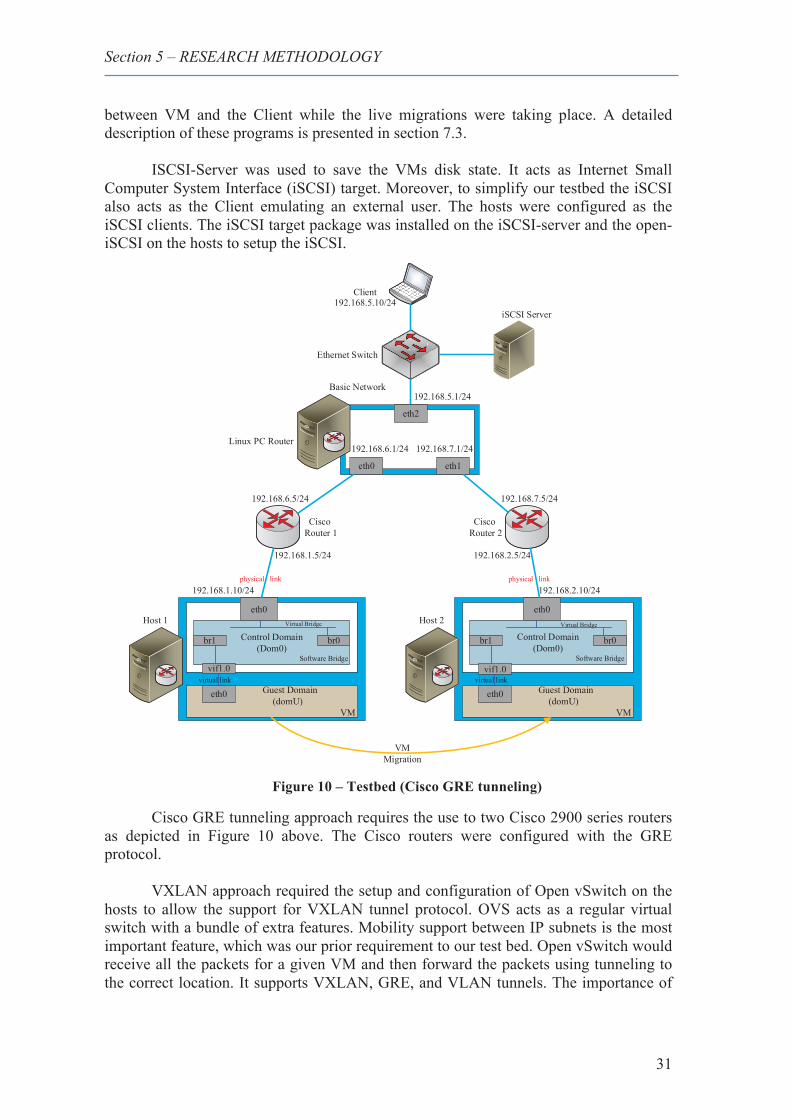
Section 5 – RESEARCH METHODOLOGY
31
between VM and the Client while the live migrations were taking place. A detailed description of these programs is presented in section 7.3.
ISCSI-Server was used to save the VMs disk state. It acts as Internet Small
Computer System Interface (iSCSI) target. Moreover, to simplify our testbed the iSCSI also acts as the Client emulating an external user. The hosts were configured as the iSCSI clients. The iSCSI target package was installed on the iSCSI-server and the open-iSCSI on the hosts to setup the iSCSI.
Figure 10 – Testbed (Cisco GRE tunneling)
Cisco GRE tunneling approach requires the use to two Cisco 2900 series routers as depicted in Figure 10 above. The Cisco routers were configured with the GRE protocol.
VXLAN approach required the setup and configuration of Open vSwitch on the
hosts to allow the support for VXLAN tunnel protocol. OVS acts as a regular virtual switch with a bundle of extra features. Mobility support between IP subnets is the most important feature, which was our prior requirement to our test bed. Open vSwitch would receive all the packets for a given VM and then forward the packets using tunneling to the correct location. It supports VXLAN, GRE, and VLAN tunnels. The importance of
eth2
eth0 eth1
Client192.168.5.10/24
iSCSI Server
192.168.5.1/24
Ethernet Switch
Basic Network
192.168.6.1/24 192.168.7.1/24Linux PC Router
Guest Domain (domU)
VM
Guest Domain (domU)
VM
eth0 eth0
VM Migration
virtual link virtual link
Control Domain(Dom0)
Software Bridgevif1.0
Control Domain(Dom0)
Software Bridgevif1.0
br1br1 br0
eth0
physical link
br0
eth0
physical link
Virtual BridgeVirtual Bridge
192.168.1.10/24 192.168.2.10/24
Host 1 Host 2
Cisco Router 1
Cisco Router 2
192.168.1.5/24
192.168.6.5/24 192.168.7.5/24
192.168.2.5/24
Section 5 – RESEARCH METHODOLOGY
32
the VXLAN technology lies in enabling the VM-VM communications and migration of hosts for different L2 subnets.
I. Hardware Configurations: • Hosts runs on Dell Intel ® Celeron ® CPU @ 2.30 GHz 64 bit laptops with
1.5GB RAM and 320GB HDD. • Linux PC router runs on the Dell AMD Athlon TM 64X2 Dual-Core processor
5000+, 64bit with 4 GB RAM and 80 GB HDD with 3 Gigabit Ethernet NICs. • iSCSI / Client runs on HP AMD AthlonTM 64 bit Processor 3500+ with 40 GB
HDD and 2 GB RAM and a Gigabit Ethernet adapter. • VM is allocated with 256-1024 MB of RAM with 1vCPU and 4GB of memory. • D-link unmanaged Switch connects Linux Pc router, ISCSI and the Client. • Two Cisco 2900 series routers were used for Cisco GRE tunneling approach.
II. VXLAN/Cisco GRE tunneling Implementation
We installed the latest Ubuntu 14.04.1 LTS OS with updated Linux kernel 3.13.0-43 generic on all the five systems used in our testbed. We implemented the latest version of Open vSwitch v2.3.0 and the Xen hypervisor v4.4, which includes full support for VXLAN and GRE tunneling protocols. Open vSwitch and VXLAN together provide the mobility between IP subnets support for migration of hosts. Open vSwitch script was modified according to our needs to work with Xen. Bi-directional VXLAN tunnels were configured between the hosts via the Linux PC router to isolate the VM traffic from the host traffic using a VNI (VXLAN identifier). Our second testbed was using the Cisco routers with GRE bidirectional tunneling between Cisco peers at the source and destination. The Cisco routers were configured with routing and tunneling protocols to enable routing between the peers over the WAN. Bi-directional tunnels were established over the Central PC router to reach the destination host. In conjunction with Open vSwitch with its mobility support, the Cisco routers were used to route traffic from a Layer 2 to Layer 3 as well maintain the network connectivity.
III. Xen Implementation
Xen is a bare metal hypervisor as described earlier. xen-hypervisor-amd64 package installs Xen 4.4-1 by default in the generic Ubuntu 14.04.1 LTS. Xen ‘conf’ file was modified to run the OVS script instead of the default Linux bridge script. The OVS script lets the OVS virtual bridges to setup the tunnel between the VTEPs.
5.2 Laboratory Scenarios We had put up two scenarios with the goal to measure the performance of the
VXLAN and Cisco GRE tunneling approaches towards live VM migration. We induced three different network RTT delay representatives namely Trans-Atlantic, Intra-Europe and Trans-Pacific. Scenarios are as follows:
• Scenario 1 - In this scenario, our goal was to measure the performance of using the VXLAN approach towards live migration. We had five Linux systems in this scenario wherein two of them acted as hosts, one as ISCSI-server; we used shared storage system, which is accessible to the hosts. The hosts act as the clients (ISCSI initiators) and the ISCSI-server is the ISCSI target. We used NetEm to emulate the WAN by inducing network delays on the interfaces of the Linux PC router. Pareto distribution was used in Netem to emulate the WAN scenario. The scenario is shown in the Figure 9.
Section 5 – RESEARCH METHODOLOGY
33
• Scenario 2 – In this scenario, our aim was to analyze and measure the performance of Cisco GRE tunneling approach towards live VM migration. Two Cisco routers were also used in this scenario between the hosts and the Linux PC router to as LDP Peers as seen in the Figure 10. We had the same ISCSI initiators and target as in scenario 1.
5.3 Performance Metrics In this section, we have discussed the performance metrics we have identified to
analyze the performance of VXLAN and GRE tunneling approaches for performing live VM migration. We have chosen four important metrics to measure the effectiveness of the approaches used in our research towards migration of VM namely service downtime, total migration time, network overhead and TCP connection survivability.
I. Service Downtime
In simple terms, downtime is referred to the period when the services running on the VM are unavailable to access to the users. In our case, the service downtime refers to the period when there is an interruption in the availability of services for the client to the VM.
A simple socket C program was developed to measure the downtime experienced
by the client. The client side (udpclient) of the program runs on client and the server side (udpserver) of the program runs on the VM. A stream of User Datagram Protocol (UDP) packets was sent from the client to the migrating VM (Figure 9/Figure 10). The program sends UDP packets for a period of every 10 ms with a payload message “VM Migrating” and a payload message “VM Migrating_Done” in the last UDP packet from client to server. The client places the sequence number and timestamp on each packet it sends to the server and the VM/server places timestamp and sequence number on the packets being received from client and also keeps track of the timestamp and sequence number placed by the client; these are used for measurements of the metrics.
In the final stage of VM migration, the VM will be suspended on the source and during this packets sent from client will be lost. The server program running on the VM will start receiving the packets once the VM has been resumed on the destination. The server keeps track of all the received packets, as a result it will discover when packet loss is encountered depending on the sequence numbers of the lost packets. The packets, which are received before and after downtime at server, are important. The difference between the timestamps of these two packets gives the downtime value.
II. Total Migration Time
The total time taken to transfer the entire state of the VM from the source to destination is expressed as the total migration time. We have used the same above tool to measure the total migration time. The tool was set to send UDP packet stream immediately after invoking VM migration command via Secure Socket Shell (SSH). The difference between the timestamp of the initial packet sent by the client and the first packet received after the downtime gives the total migration time. It includes the time taken by the approaches used to maintain the network connectivity.
Section 5 – RESEARCH METHODOLOGY
34
III. Network Overhead In simple terms, overhead refers to anything in excess or indirect computation
time, memory, bandwidth, or other resources. The amount of VXLAN/GRE traffic may cause significant network overhead depending on the rate at which the VM migration is taking place. We measured the amount of traffic crossing the Ethernet interfaces namely eth0 and eth1 of Linux PC router using tshark tool during live VM migration. The captured traffic generated by Xen and the amount of traffic generated using GRE/VXLAN are analyzed and compared.
IV. TCP Connection sustainability
We scrutinized the Transmission Control Protocol (TCP) connections established between the client and the VM migrating. The main task here is to check if the TCP connection between external user (client in Figure 9 / Figure 10) and migrating VM (VM in Figure 9 / Figure 10) is survived before and after the migration. A simple socket program in C language was written to analyze the sustainability of such TCP connections in order to maintain the network connectivity during and after migration. The client side (tcpclient) of the program runs on VM and the server side (tcpserver) of the program runs on the client. The server creates a TCP stream socket and listens for the request connection from client. Once the connection is made, the client send a stream of TCP packets to server at a period of every 10 ms and the server receives the packets. We have used recv() Linux function in the program for receiving the packets. The function returns a zero value if the connection is terminated between client and VM or returns -1 in case of error or else upon successful completion of packet, returns the length of the message in bytes. Therefore, we can consider that the TCP connection is survived after migration if the Linux recv() routine doesn’t encounter zero or -1. Otherwise, the TCP connection is interrupted.
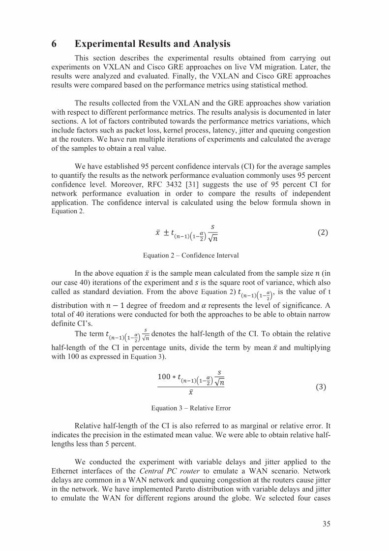
35
6 Experimental Results and Analysis This section describes the experimental results obtained from carrying out
experiments on VXLAN and Cisco GRE approaches on live VM migration. Later, the results were analyzed and evaluated. Finally, the VXLAN and Cisco GRE approaches results were compared based on the performance metrics using statistical method.
The results collected from the VXLAN and the GRE approaches show variation
with respect to different performance metrics. The results analysis is documented in later sections. A lot of factors contributed towards the performance metrics variations, which include factors such as packet loss, kernel process, latency, jitter and queuing congestion at the routers. We have run multiple iterations of experiments and calculated the average of the samples to obtain a real value.
We have established 95 percent confidence intervals (CI) for the average samples
to quantify the results as the network performance evaluation commonly uses 95 percent confidence level. Moreover, RFC 3432 [31] suggests the use of 95 percent CI for network performance evaluation in order to compare the results of independent application. The confidence interval is calculated using the below formula shown in Equation 2.
Equation 2 – Confidence Interval
In the above equation is the sample mean calculated from the sample size (in
our case 40) iterations of the experiment and is the square root of variance, which also called as standard deviation. From the above Equation 2) , is the value of t
distribution with degree of freedom and represents the level of significance. A total of 40 iterations were conducted for both the approaches to be able to obtain narrow definite CI’s.
The term denotes the half-length of the CI. To obtain the relative
half-length of the CI in percentage units, divide the term by mean and multiplying with 100 as expressed in Equation 3).
Equation 3 – Relative Error Relative half-length of the CI is also referred to as marginal or relative error. It
indicates the precision in the estimated mean value. We were able to obtain relative half-lengths less than 5 percent.
We conducted the experiment with variable delays and jitter applied to the
Ethernet interfaces of the Central PC router to emulate a WAN scenario. Network delays are common in a WAN network and queuing congestion at the routers cause jitter in the network. We have implemented Pareto distribution with variable delays and jitter to emulate the WAN for different regions around the globe. We selected four cases
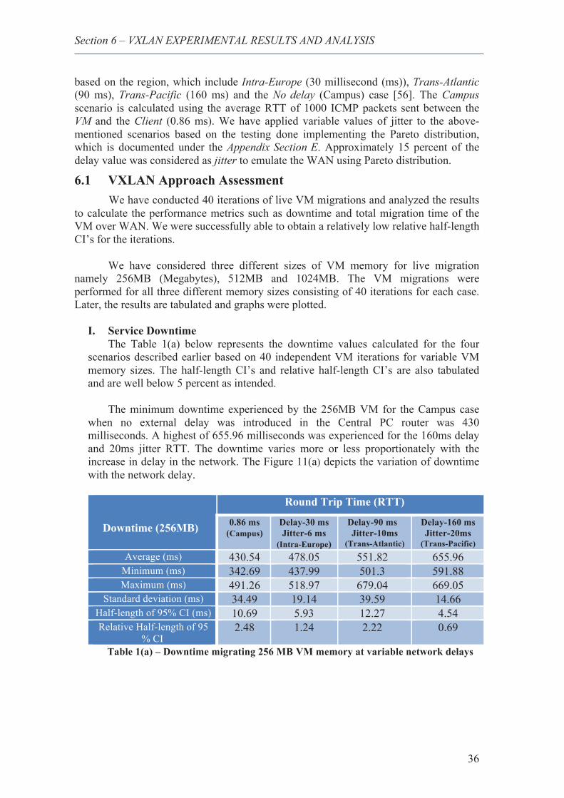
Section 6 – VXLAN EXPERIMENTAL RESULTS AND ANALYSIS
36
based on the region, which include Intra-Europe (30 millisecond (ms)), Trans-Atlantic (90 ms), Trans-Pacific (160 ms) and the No delay (Campus) case [56]. The Campus scenario is calculated using the average RTT of 1000 ICMP packets sent between the VM and the Client (0.86 ms). We have applied variable values of jitter to the above-mentioned scenarios based on the testing done implementing the Pareto distribution, which is documented under the Appendix Section E. Approximately 15 percent of the delay value was considered as jitter to emulate the WAN using Pareto distribution.
6.1 VXLAN Approach Assessment We have conducted 40 iterations of live VM migrations and analyzed the results
to calculate the performance metrics such as downtime and total migration time of the VM over WAN. We were successfully able to obtain a relatively low relative half-length CI’s for the iterations.
We have considered three different sizes of VM memory for live migration namely 256MB (Megabytes), 512MB and 1024MB. The VM migrations were performed for all three different memory sizes consisting of 40 iterations for each case. Later, the results are tabulated and graphs were plotted.
I. Service Downtime
The Table 1(a) below represents the downtime values calculated for the four scenarios described earlier based on 40 independent VM iterations for variable VM memory sizes. The half-length CI’s and relative half-length CI’s are also tabulated and are well below 5 percent as intended.
The minimum downtime experienced by the 256MB VM for the Campus case
when no external delay was introduced in the Central PC router was 430 milliseconds. A highest of 655.96 milliseconds was experienced for the 160ms delay and 20ms jitter RTT. The downtime varies more or less proportionately with the increase in delay in the network. The Figure 11(a) depicts the variation of downtime with the network delay.
Downtime (256MB)
Round Trip Time (RTT)
0.86 ms (Campus)
Delay-30 ms Jitter-6 ms
(Intra-Europe)
Delay-90 ms Jitter-10ms
(Trans-Atlantic)
Delay-160 ms Jitter-20ms
(Trans-Pacific) Average (ms) 430.54 478.05 551.82 655.96
Minimum (ms) 342.69 437.99 501.3 591.88 Maximum (ms) 491.26 518.97 679.04 669.05
Standard deviation (ms) 34.49 19.14 39.59 14.66 Half-length of 95% CI (ms) 10.69 5.93 12.27 4.54 Relative Half-length of 95
% CI 2.48 1.24 2.22 0.69
Table 1(a) – Downtime migrating 256 MB VM memory at variable network delays
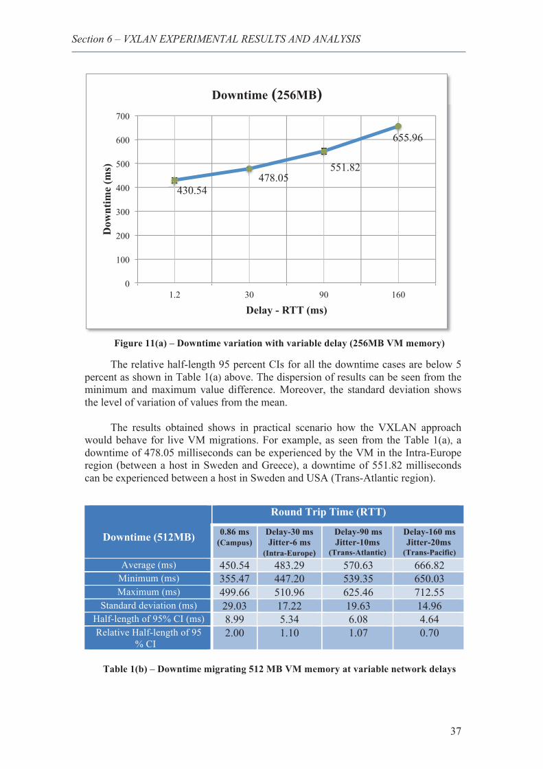
Section 6 – VXLAN EXPERIMENTAL RESULTS AND ANALYSIS
37
Figure 11(a) – Downtime variation with variable delay (256MB VM memory)
The relative half-length 95 percent CIs for all the downtime cases are below 5 percent as shown in Table 1(a) above. The dispersion of results can be seen from the minimum and maximum value difference. Moreover, the standard deviation shows the level of variation of values from the mean.
The results obtained shows in practical scenario how the VXLAN approach
would behave for live VM migrations. For example, as seen from the Table 1(a), a downtime of 478.05 milliseconds can be experienced by the VM in the Intra-Europe region (between a host in Sweden and Greece), a downtime of 551.82 milliseconds can be experienced between a host in Sweden and USA (Trans-Atlantic region).
Table 1(b) – Downtime migrating 512 MB VM memory at variable network delays
430.54 478.05
551.82
655.96
0
100
200
300
400
500
600
700
1.2 30 90 160
Dow
ntim
e (m
s)
Delay - RTT (ms)
Downtime (256MB)
Downtime (512MB)
Round Trip Time (RTT)
0.86 ms (Campus)
Delay-30 ms Jitter-6 ms
(Intra-Europe)
Delay-90 ms Jitter-10ms
(Trans-Atlantic)
Delay-160 ms Jitter-20ms
(Trans-Pacific) Average (ms) 450.54 483.29 570.63 666.82
Minimum (ms) 355.47 447.20 539.35 650.03 Maximum (ms) 499.66 510.96 625.46 712.55
Standard deviation (ms) 29.03 17.22 19.63 14.96 Half-length of 95% CI (ms) 8.99 5.34 6.08 4.64 Relative Half-length of 95
% CI 2.00 1.10 1.07 0.70
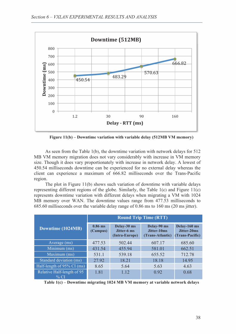
Section 6 – VXLAN EXPERIMENTAL RESULTS AND ANALYSIS
38
Figure 11(b) – Downtime variation with variable delay (512MB VM memory)
As seen from the Table 1(b), the downtime variation with network delays for 512
MB VM memory migration does not vary considerably with increase in VM memory size. Though it does vary proportionately with increase in network delay. A lowest of 450.54 milliseconds downtime can be experienced for no external delay whereas the client can experience a maximum of 666.82 milliseconds over the Trans-Pacific region.
The plot in Figure 11(b) shows such variation of downtime with variable delays representing different regions of the globe. Similarly, the Table 1(c) and Figure 11(c) represents downtime variation with different delays when migrating a VM with 1024 MB memory over WAN. The downtime values range from 477.53 milliseconds to 685.60 milliseconds over the variable delay range of 0.86 ms to 160 ms (20 ms jitter).
Downtime (1024MB)
Round Trip Time (RTT)
0.86 ms (Campus)
Delay-30 ms Jitter-6 ms
(Intra-Europe)
Delay-90 ms Jitter-10ms
(Trans-Atlantic)
Delay-160 ms Jitter-20ms
(Trans-Pacific)
Average (ms) 477.53 502.44 607.17 685.60 Minimum (ms) 431.54 455.94 581.01 662.51 Maximum (ms) 531.1 539.18 655.52 712.78
Standard deviation (ms) 27.92 18.21 18.18 14.95 Half-length of 95% CI (ms) 8.65 5.64 5.63 4.63 Relative Half-length of 95
% CI 1.81 1.12 0.92 0.68
Table 1(c) – Downtime migrating 1024 MB VM memory at variable network delays
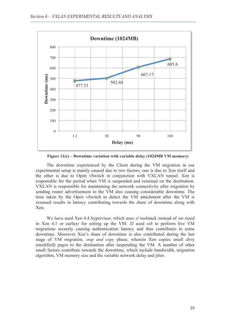
Section 6 – VXLAN EXPERIMENTAL RESULTS AND ANALYSIS
39
Figure 11(c) – Downtime variation with variable delay (1024MB VM memory)
The downtime experienced by the Client during the VM migration in our experimental setup is mainly caused due to two factors; one is due to Xen itself and the other is due to Open vSwitch in conjunction with VXLAN tunnel. Xen is responsible for the period when VM is suspended and resumed on the destination. VXLAN is responsible for maintaining the network connectivity after migration by sending router advertisement to the VM also causing considerable downtime. The time taken by the Open vSwitch to detect the VM attachment after the VM is resumed results in latency contributing towards the share of downtime along with Xen.
We have used Xen 4.4 hypervisor, which uses xl toolstack instead of xm (used
in Xen 4.1 or earlier) for setting up the VM. Xl used ssh to perform live VM migrations securely causing authentication latency and thus contributes to some downtime. Moreover Xen’s share of downtime is also contributed during the last stage of VM migration, stop and copy phase, wherein Xen copies small dirty (modified) pages to the destination after suspending the VM. A number of other small factors contribute towards the downtime, which include bandwidth, migration algorithm, VM memory size and the variable network delay and jitter.
477.53 502.44
607.17
685.6
0
100
200
300
400
500
600
700
800
1.2 30 90 160
Dow
ntim
e (m
s)
Delay (ms)
Downtime (1024MB)
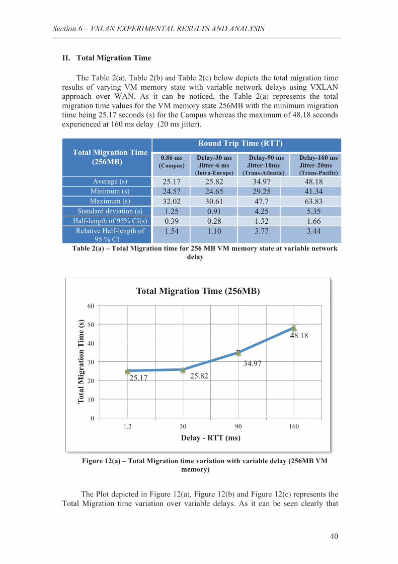
Section 6 – VXLAN EXPERIMENTAL RESULTS AND ANALYSIS
40
II. Total Migration Time
The Table 2(a), Table 2(b) and Table 2(c) below depicts the total migration time results of varying VM memory state with variable network delays using VXLAN approach over WAN. As it can be noticed, the Table 2(a) represents the total migration time values for the VM memory state 256MB with the minimum migration time being 25.17 seconds (s) for the Campus whereas the maximum of 48.18 seconds experienced at 160 ms delay (20 ms jitter).
Total Migration Time (256MB)
Round Trip Time (RTT)
0.86 ms (Campus)
Delay-30 ms Jitter-6 ms
(Intra-Europe)
Delay-90 ms Jitter-10ms
(Trans-Atlantic)
Delay-160 ms Jitter-20ms (Trans-Pacific)
Average (s) 25.17 25.82 34.97 48.18 Minimum (s) 24.57 24.65 29.25 41.34 Maximum (s) 32.02 30.61 47.7 63.83
Standard deviation (s) 1.25 0.91 4.25 5.35 Half-length of 95% CI(s) 0.39 0.28 1.32 1.66 Relative Half-length of
95 % CI 1.54 1.10 3.77 3.44
Table 2(a) – Total Migration time for 256 MB VM memory state at variable network delay
Figure 12(a) – Total Migration time variation with variable delay (256MB VM
memory)
The Plot depicted in Figure 12(a), Figure 12(b) and Figure 12(c) represents the
Total Migration time variation over variable delays. As it can be seen clearly that
25.17 25.82 34.97
48.18
0
10
20
30
40
50
60
1.2 30 90 160
Tota
l Mig
ratio
n Ti
me
(s)
Delay - RTT (ms)
Total Migration Time (256MB)
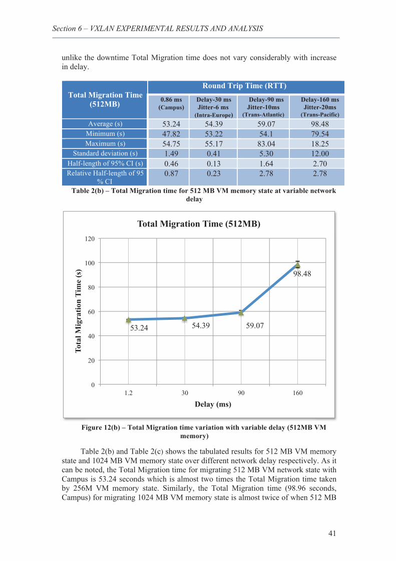
Section 6 – VXLAN EXPERIMENTAL RESULTS AND ANALYSIS
41
unlike the downtime Total Migration time does not vary considerably with increase in delay.
Total Migration Time (512MB)
Round Trip Time (RTT)
0.86 ms (Campus)
Delay-30 ms Jitter-6 ms
(Intra-Europe)
Delay-90 ms Jitter-10ms
(Trans-Atlantic)
Delay-160 ms Jitter-20ms
(Trans-Pacific) Average (s) 53.24 54.39 59.07 98.48
Minimum (s) 47.82 53.22 54.1 79.54 Maximum (s) 54.75 55.17 83.04 18.25
Standard deviation (s) 1.49 0.41 5.30 12.00 Half-length of 95% CI (s) 0.46 0.13 1.64 2.70 Relative Half-length of 95
% CI 0.87 0.23 2.78 2.78
Table 2(b) – Total Migration time for 512 MB VM memory state at variable network delay
Figure 12(b) – Total Migration time variation with variable delay (512MB VM
memory)
Table 2(b) and Table 2(c) shows the tabulated results for 512 MB VM memory state and 1024 MB VM memory state over different network delay respectively. As it can be noted, the Total Migration time for migrating 512 MB VM network state with Campus is 53.24 seconds which is almost two times the Total Migration time taken by 256M VM memory state. Similarly, the Total Migration time (98.96 seconds, Campus) for migrating 1024 MB VM memory state is almost twice of when 512 MB
53.24 54.39 59.07
98.48
0
20
40
60
80
100
120
1.2 30 90 160
Tota
l Mig
ratio
n Ti
me
(s)
Delay (ms)
Total Migration Time (512MB)
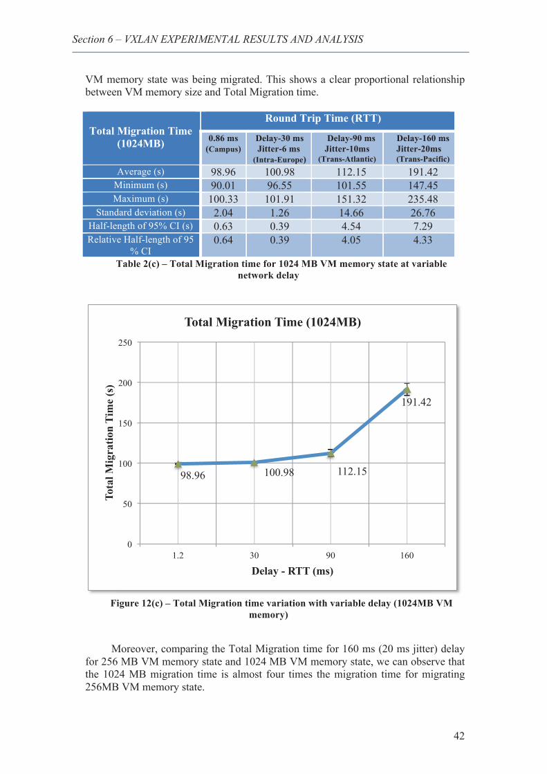
Section 6 – VXLAN EXPERIMENTAL RESULTS AND ANALYSIS
42
VM memory state was being migrated. This shows a clear proportional relationship between VM memory size and Total Migration time.
Total Migration Time (1024MB)
Round Trip Time (RTT)
0.86 ms (Campus)
Delay-30 ms Jitter-6 ms
(Intra-Europe)
Delay-90 ms Jitter-10ms
(Trans-Atlantic)
Delay-160 ms Jitter-20ms (Trans-Pacific)
Average (s) 98.96 100.98 112.15 191.42 Minimum (s) 90.01 96.55 101.55 147.45 Maximum (s) 100.33 101.91 151.32 235.48
Standard deviation (s) 2.04 1.26 14.66 26.76 Half-length of 95% CI (s) 0.63 0.39 4.54 7.29 Relative Half-length of 95
% CI 0.64 0.39 4.05 4.33
Table 2(c) – Total Migration time for 1024 MB VM memory state at variable network delay
Figure 12(c) – Total Migration time variation with variable delay (1024MB VM
memory)
Moreover, comparing the Total Migration time for 160 ms (20 ms jitter) delay
for 256 MB VM memory state and 1024 MB VM memory state, we can observe that the 1024 MB migration time is almost four times the migration time for migrating 256MB VM memory state.
98.96 100.98 112.15
191.42
0
50
100
150
200
250
1.2 30 90 160
Tota
l Mig
ratio
n Ti
me
(s)
Delay - RTT (ms)
Total Migration Time (1024MB)
Section 6 – VXLAN EXPERIMENTAL RESULTS AND ANALYSIS
43
Considering the VM disk state being a shared storage medium, the total migration time mainly shows its dependence on memory, network and CPU state which was expected. We have observed a sudden increase in total migration time when the delay is increased from 90 ms to 160 ms unlike the case when the delay is changed from 30 ms to 90 ms, which showed a gradual increase. On an average, we could observe an increase of about 58 percent in total migration time between the 90 ms delay and 160 ms delay. In general, Xen uses TCP connection to transfer memory states. Bandwidth and network delay play an important role for TCP performance, which deteriorates when the buffer space gets full. Thus, a prolonged migration time will be experienced as seen from our results.
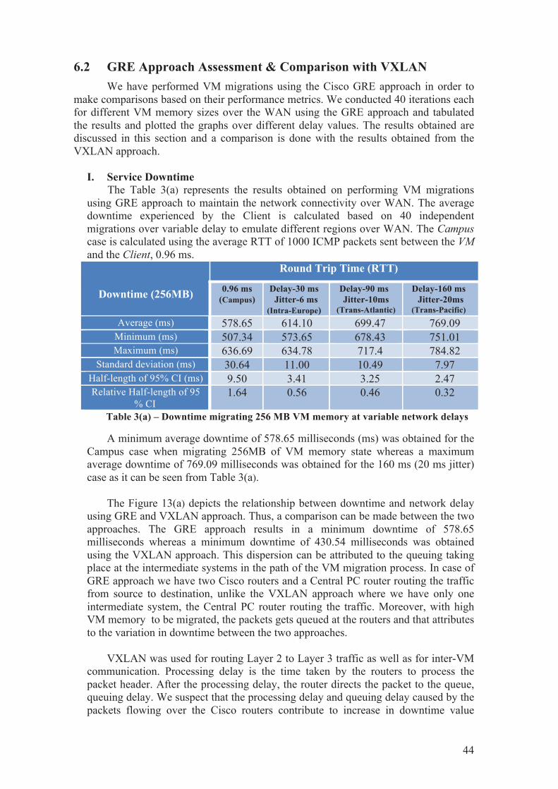
44
6.2 GRE Approach Assessment & Comparison with VXLAN We have performed VM migrations using the Cisco GRE approach in order to
make comparisons based on their performance metrics. We conducted 40 iterations each for different VM memory sizes over the WAN using the GRE approach and tabulated the results and plotted the graphs over different delay values. The results obtained are discussed in this section and a comparison is done with the results obtained from the VXLAN approach.
I. Service Downtime
The Table 3(a) represents the results obtained on performing VM migrations using GRE approach to maintain the network connectivity over WAN. The average downtime experienced by the Client is calculated based on 40 independent migrations over variable delay to emulate different regions over WAN. The Campus case is calculated using the average RTT of 1000 ICMP packets sent between the VM and the Client, 0.96 ms.
Downtime (256MB)
Round Trip Time (RTT)
0.96 ms (Campus)
Delay-30 ms Jitter-6 ms
(Intra-Europe)
Delay-90 ms Jitter-10ms
(Trans-Atlantic)
Delay-160 ms Jitter-20ms
(Trans-Pacific) Average (ms) 578.65 614.10 699.47 769.09
Minimum (ms) 507.34 573.65 678.43 751.01 Maximum (ms) 636.69 634.78 717.4 784.82
Standard deviation (ms) 30.64 11.00 10.49 7.97 Half-length of 95% CI (ms) 9.50 3.41 3.25 2.47 Relative Half-length of 95
% CI 1.64 0.56 0.46 0.32
Table 3(a) – Downtime migrating 256 MB VM memory at variable network delays
A minimum average downtime of 578.65 milliseconds (ms) was obtained for the Campus case when migrating 256MB of VM memory state whereas a maximum average downtime of 769.09 milliseconds was obtained for the 160 ms (20 ms jitter) case as it can be seen from Table 3(a).
The Figure 13(a) depicts the relationship between downtime and network delay
using GRE and VXLAN approach. Thus, a comparison can be made between the two approaches. The GRE approach results in a minimum downtime of 578.65 milliseconds whereas a minimum downtime of 430.54 milliseconds was obtained using the VXLAN approach. This dispersion can be attributed to the queuing taking place at the intermediate systems in the path of the VM migration process. In case of GRE approach we have two Cisco routers and a Central PC router routing the traffic from source to destination, unlike the VXLAN approach where we have only one intermediate system, the Central PC router routing the traffic. Moreover, with high VM memory to be migrated, the packets gets queued at the routers and that attributes to the variation in downtime between the two approaches.
VXLAN was used for routing Layer 2 to Layer 3 traffic as well as for inter-VM
communication. Processing delay is the time taken by the routers to process the packet header. After the processing delay, the router directs the packet to the queue, queuing delay. We suspect that the processing delay and queuing delay caused by the packets flowing over the Cisco routers contribute to increase in downtime value
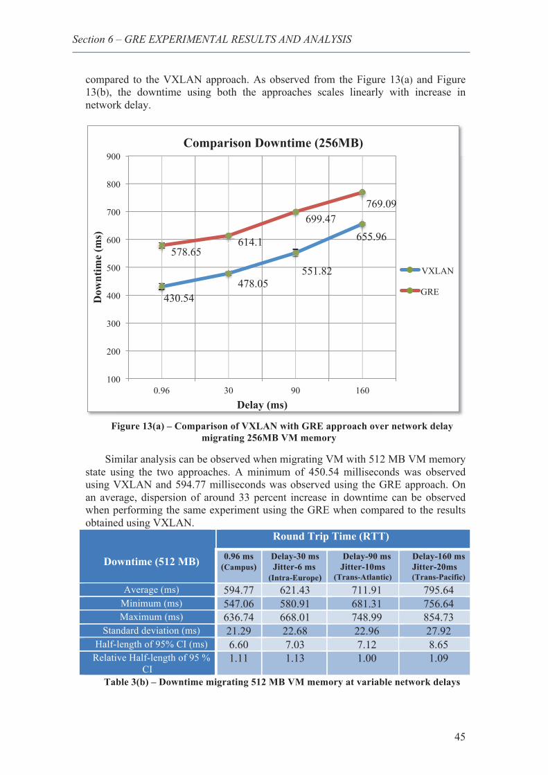
Section 6 – GRE EXPERIMENTAL RESULTS AND ANALYSIS
45
compared to the VXLAN approach. As observed from the Figure 13(a) and Figure 13(b), the downtime using both the approaches scales linearly with increase in network delay.
Figure 13(a) – Comparison of VXLAN with GRE approach over network delay
migrating 256MB VM memory
Similar analysis can be observed when migrating VM with 512 MB VM memory state using the two approaches. A minimum of 450.54 milliseconds was observed using VXLAN and 594.77 milliseconds was observed using the GRE approach. On an average, dispersion of around 33 percent increase in downtime can be observed when performing the same experiment using the GRE when compared to the results obtained using VXLAN.
Downtime (512 MB)
Round Trip Time (RTT)
0.96 ms (Campus)
Delay-30 ms Jitter-6 ms
(Intra-Europe)
Delay-90 ms Jitter-10ms
(Trans-Atlantic)
Delay-160 ms Jitter-20ms (Trans-Pacific)
Average (ms) 594.77 621.43 711.91 795.64 Minimum (ms) 547.06 580.91 681.31 756.64 Maximum (ms) 636.74 668.01 748.99 854.73
Standard deviation (ms) 21.29 22.68 22.96 27.92 Half-length of 95% CI (ms) 6.60 7.03 7.12 8.65
Relative Half-length of 95 % CI
1.11 1.13 1.00 1.09
Table 3(b) – Downtime migrating 512 MB VM memory at variable network delays
430.54 478.05
551.82
655.96 578.65
614.1
699.47 769.09
100
200
300
400
500
600
700
800
900
0.96 30 90 160
Dow
ntim
e (m
s)
Delay (ms)
Comparison Downtime (256MB)
VXLAN
GRE
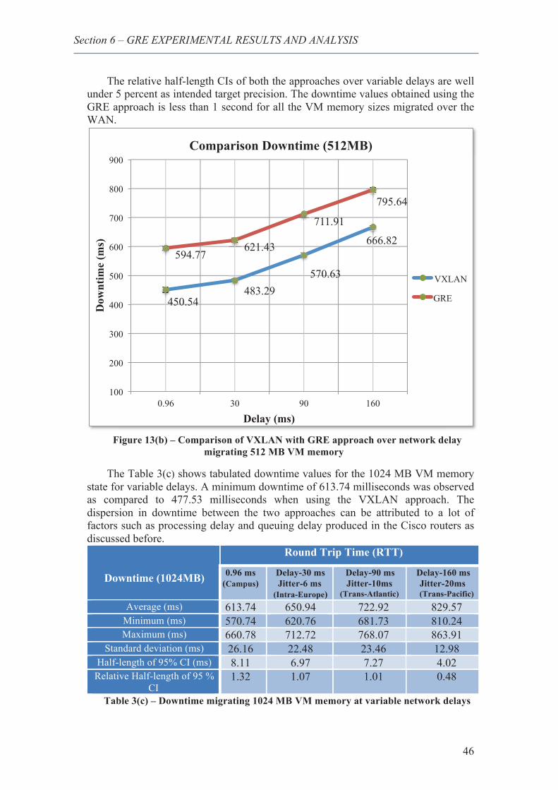
Section 6 – GRE EXPERIMENTAL RESULTS AND ANALYSIS
46
The relative half-length CIs of both the approaches over variable delays are well under 5 percent as intended target precision. The downtime values obtained using the GRE approach is less than 1 second for all the VM memory sizes migrated over the WAN.
Figure 13(b) – Comparison of VXLAN with GRE approach over network delay
migrating 512 MB VM memory
The Table 3(c) shows tabulated downtime values for the 1024 MB VM memory state for variable delays. A minimum downtime of 613.74 milliseconds was observed as compared to 477.53 milliseconds when using the VXLAN approach. The dispersion in downtime between the two approaches can be attributed to a lot of factors such as processing delay and queuing delay produced in the Cisco routers as discussed before.
Downtime (1024MB)
Round Trip Time (RTT)
0.96 ms (Campus)
Delay-30 ms Jitter-6 ms
(Intra-Europe)
Delay-90 ms Jitter-10ms
(Trans-Atlantic)
Delay-160 ms Jitter-20ms (Trans-Pacific)
Average (ms) 613.74 650.94 722.92 829.57 Minimum (ms) 570.74 620.76 681.73 810.24 Maximum (ms) 660.78 712.72 768.07 863.91
Standard deviation (ms) 26.16 22.48 23.46 12.98 Half-length of 95% CI (ms) 8.11 6.97 7.27 4.02
Relative Half-length of 95 % CI
1.32 1.07 1.01 0.48
Table 3(c) – Downtime migrating 1024 MB VM memory at variable network delays
450.54 483.29
570.63
666.82 594.77
621.43
711.91
795.64
100
200
300
400
500
600
700
800
900
0.96 30 90 160
Dow
ntim
e (m
s)
Delay (ms)
Comparison Downtime (512MB)
VXLAN
GRE
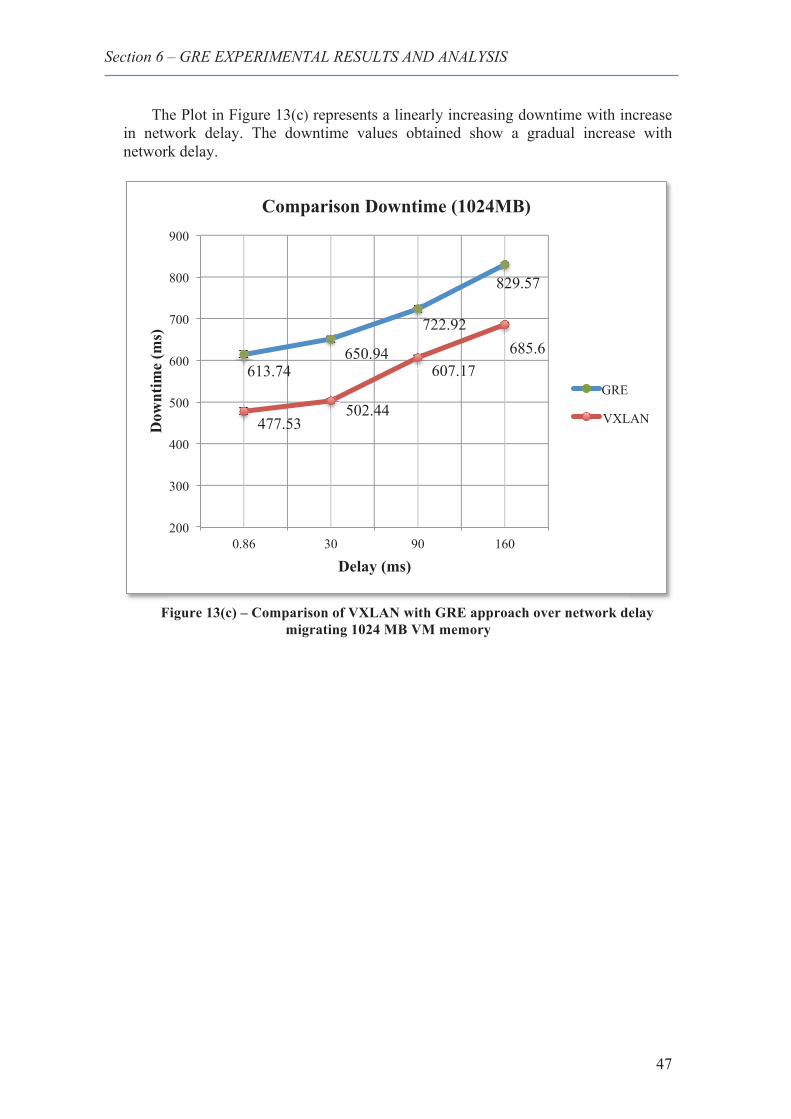
Section 6 – GRE EXPERIMENTAL RESULTS AND ANALYSIS
47
The Plot in Figure 13(c) represents a linearly increasing downtime with increase in network delay. The downtime values obtained show a gradual increase with network delay.
Figure 13(c) – Comparison of VXLAN with GRE approach over network delay
migrating 1024 MB VM memory
613.74 650.94
722.92
829.57
477.53 502.44
607.17 685.6
200
300
400
500
600
700
800
900
0.86 30 90 160
Dow
ntim
e (m
s)
Delay (ms)
Comparison Downtime (1024MB)
GRE
VXLAN
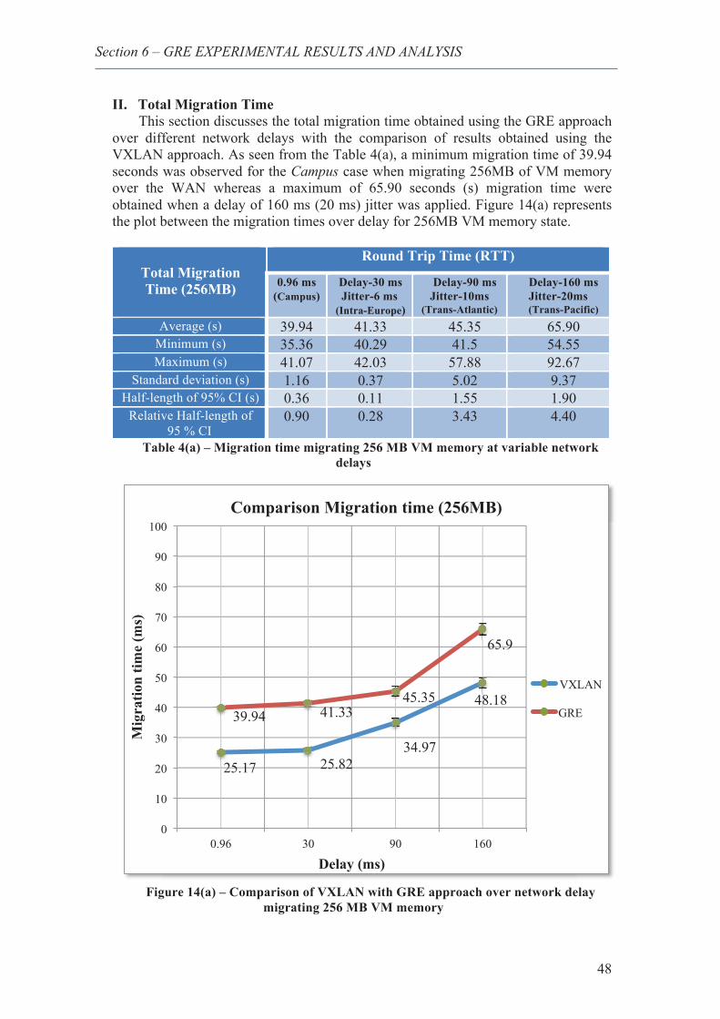
Section 6 – GRE EXPERIMENTAL RESULTS AND ANALYSIS
48
II. Total Migration Time This section discusses the total migration time obtained using the GRE approach
over different network delays with the comparison of results obtained using the VXLAN approach. As seen from the Table 4(a), a minimum migration time of 39.94 seconds was observed for the Campus case when migrating 256MB of VM memory over the WAN whereas a maximum of 65.90 seconds (s) migration time were obtained when a delay of 160 ms (20 ms) jitter was applied. Figure 14(a) represents the plot between the migration times over delay for 256MB VM memory state.
Total Migration Time (256MB)
Round Trip Time (RTT)
0.96 ms (Campus)
Delay-30 ms Jitter-6 ms
(Intra-Europe)
Delay-90 ms Jitter-10ms
(Trans-Atlantic)
Delay-160 ms Jitter-20ms (Trans-Pacific)
Average (s) 39.94 41.33 45.35 65.90 Minimum (s) 35.36 40.29 41.5 54.55 Maximum (s) 41.07 42.03 57.88 92.67
Standard deviation (s) 1.16 0.37 5.02 9.37 Half-length of 95% CI (s) 0.36 0.11 1.55 1.90
Relative Half-length of 95 % CI
0.90 0.28 3.43 4.40
Table 4(a) – Migration time migrating 256 MB VM memory at variable network delays
Figure 14(a) – Comparison of VXLAN with GRE approach over network delay
migrating 256 MB VM memory
25.17 25.82 34.97
48.18 39.94 41.33
45.35
65.9
0
10
20
30
40
50
60
70
80
90
100
0.96 30 90 160
Mig
ratio
n tim
e (m
s)
Delay (ms)
Comparison Migration time (256MB)
VXLAN
GRE
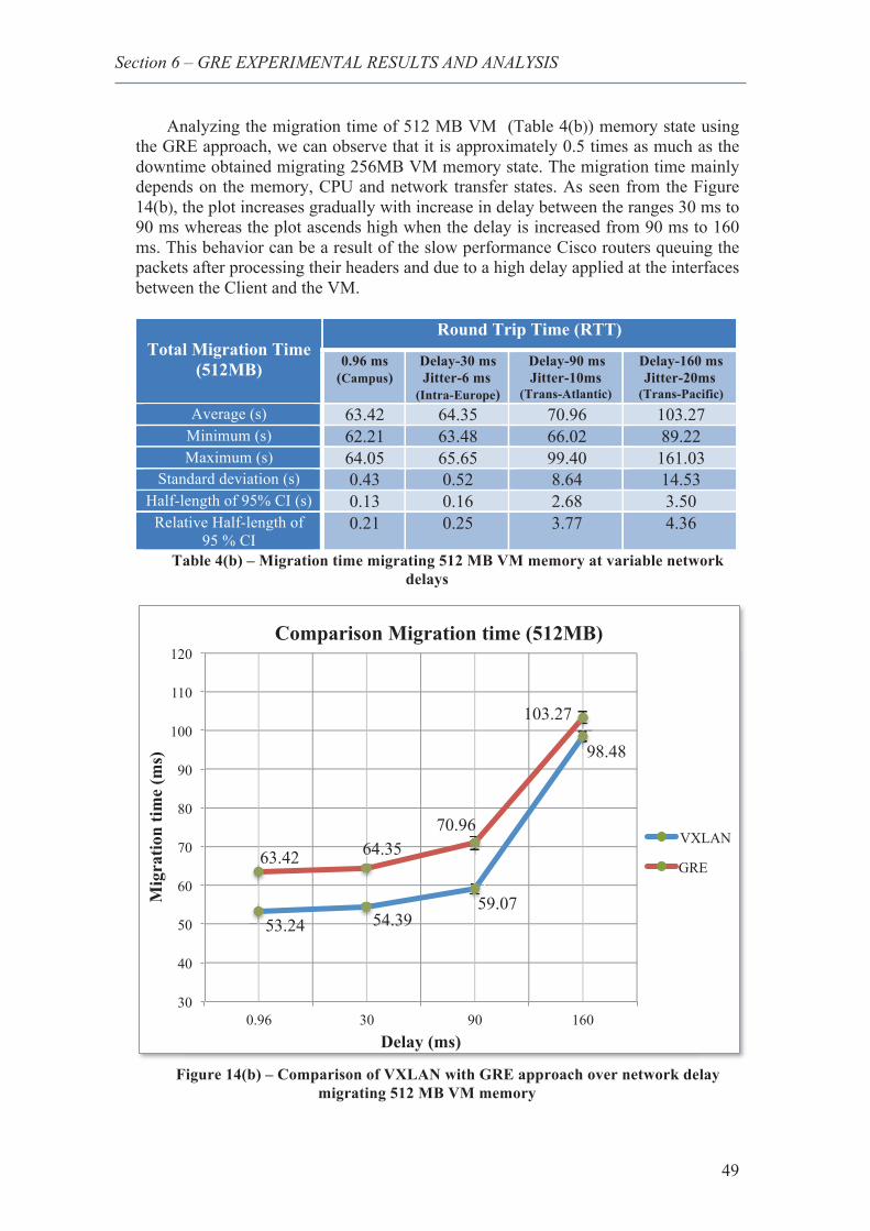
Section 6 – GRE EXPERIMENTAL RESULTS AND ANALYSIS
49
Analyzing the migration time of 512 MB VM (Table 4(b)) memory state using the GRE approach, we can observe that it is approximately 0.5 times as much as the downtime obtained migrating 256MB VM memory state. The migration time mainly depends on the memory, CPU and network transfer states. As seen from the Figure 14(b), the plot increases gradually with increase in delay between the ranges 30 ms to 90 ms whereas the plot ascends high when the delay is increased from 90 ms to 160 ms. This behavior can be a result of the slow performance Cisco routers queuing the packets after processing their headers and due to a high delay applied at the interfaces between the Client and the VM.
Total Migration Time (512MB)
Round Trip Time (RTT)
0.96 ms (Campus)
Delay-30 ms Jitter-6 ms
(Intra-Europe)
Delay-90 ms Jitter-10ms
(Trans-Atlantic)
Delay-160 ms Jitter-20ms
(Trans-Pacific) Average (s) 63.42 64.35 70.96 103.27
Minimum (s) 62.21 63.48 66.02 89.22 Maximum (s) 64.05 65.65 99.40 161.03
Standard deviation (s) 0.43 0.52 8.64 14.53 Half-length of 95% CI (s) 0.13 0.16 2.68 3.50
Relative Half-length of 95 % CI
0.21 0.25 3.77 4.36
Table 4(b) – Migration time migrating 512 MB VM memory at variable network delays
Figure 14(b) – Comparison of VXLAN with GRE approach over network delay
migrating 512 MB VM memory
53.24 54.39 59.07
98.48
63.42 64.35 70.96
103.27
30
40
50
60
70
80
90
100
110
120
0.96 30 90 160
Mig
ratio
n tim
e (m
s)
Delay (ms)
Comparison Migration time (512MB)
VXLAN
GRE
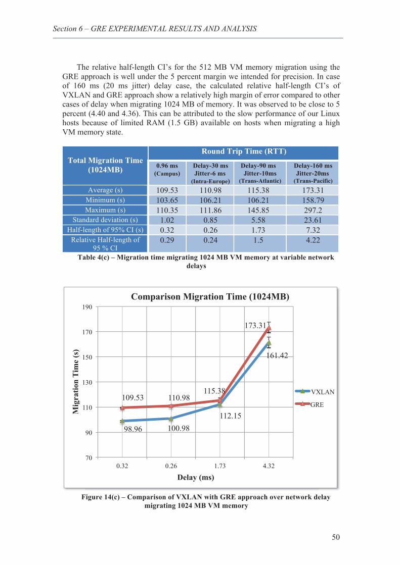
Section 6 – GRE EXPERIMENTAL RESULTS AND ANALYSIS
50
The relative half-length CI’s for the 512 MB VM memory migration using the
GRE approach is well under the 5 percent margin we intended for precision. In case of 160 ms (20 ms jitter) delay case, the calculated relative half-length CI’s of VXLAN and GRE approach show a relatively high margin of error compared to other cases of delay when migrating 1024 MB of memory. It was observed to be close to 5 percent (4.40 and 4.36). This can be attributed to the slow performance of our Linux hosts because of limited RAM (1.5 GB) available on hosts when migrating a high VM memory state.
Total Migration Time (1024MB)
Round Trip Time (RTT)
0.96 ms (Campus)
Delay-30 ms Jitter-6 ms
(Intra-Europe)
Delay-90 ms Jitter-10ms
(Trans-Atlantic)
Delay-160 ms Jitter-20ms
(Trans-Pacific) Average (s) 109.53 110.98 115.38 173.31
Minimum (s) 103.65 106.21 106.21 158.79 Maximum (s) 110.35 111.86 145.85 297.2
Standard deviation (s) 1.02 0.85 5.58 23.61 Half-length of 95% CI (s) 0.32 0.26 1.73 7.32
Relative Half-length of 95 % CI
0.29 0.24 1.5 4.22
Table 4(c) – Migration time migrating 1024 MB VM memory at variable network delays
Figure 14(c) – Comparison of VXLAN with GRE approach over network delay
migrating 1024 MB VM memory
98.96 100.98 112.15
161.42
109.53 110.98 115.38
173.31
70
90
110
130
150
170
190
0.32 0.26 1.73 4.32
Mig
ratio
n Ti
me
(s)
Delay (ms)
Comparison Migration Time (1024MB)
VXLAN
GRE
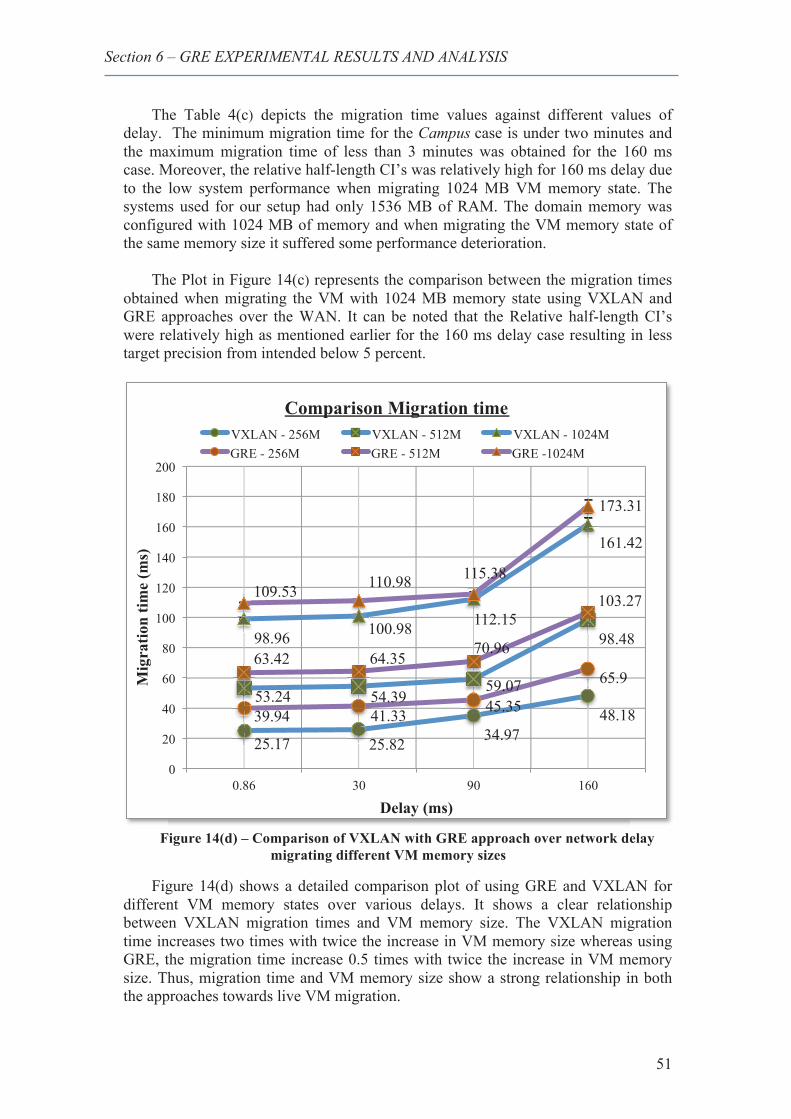
Section 6 – GRE EXPERIMENTAL RESULTS AND ANALYSIS
51
The Table 4(c) depicts the migration time values against different values of delay. The minimum migration time for the Campus case is under two minutes and the maximum migration time of less than 3 minutes was obtained for the 160 ms case. Moreover, the relative half-length CI’s was relatively high for 160 ms delay due to the low system performance when migrating 1024 MB VM memory state. The systems used for our setup had only 1536 MB of RAM. The domain memory was configured with 1024 MB of memory and when migrating the VM memory state of the same memory size it suffered some performance deterioration.
The Plot in Figure 14(c) represents the comparison between the migration times
obtained when migrating the VM with 1024 MB memory state using VXLAN and GRE approaches over the WAN. It can be noted that the Relative half-length CI’s were relatively high as mentioned earlier for the 160 ms delay case resulting in less target precision from intended below 5 percent.
Figure 14(d) – Comparison of VXLAN with GRE approach over network delay
migrating different VM memory sizes
Figure 14(d) shows a detailed comparison plot of using GRE and VXLAN for different VM memory states over various delays. It shows a clear relationship between VXLAN migration times and VM memory size. The VXLAN migration time increases two times with twice the increase in VM memory size whereas using GRE, the migration time increase 0.5 times with twice the increase in VM memory size. Thus, migration time and VM memory size show a strong relationship in both the approaches towards live VM migration.
25.17 25.82 34.97 48.18
53.24 54.39 59.07
98.48 98.96 100.98 112.15
161.42
39.94 41.33 45.35
65.9 63.42 64.35
70.96
103.27 109.53 110.98 115.38
173.31
0
20
40
60
80
100
120
140
160
180
200
0.86 30 90 160
Mig
ratio
n tim
e (m
s)
Delay (ms)
Comparison Migration time VXLAN - 256M VXLAN - 512M VXLAN - 1024M GRE - 256M GRE - 512M GRE -1024M
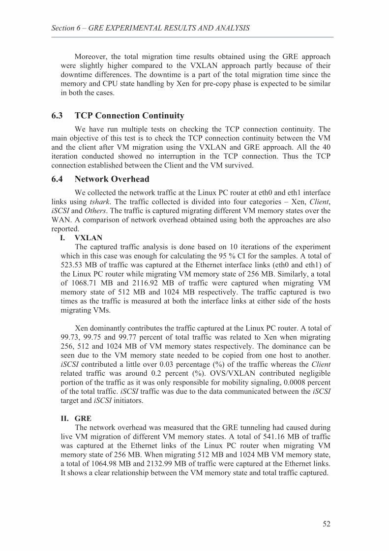
Section 6 – GRE EXPERIMENTAL RESULTS AND ANALYSIS
52
Moreover, the total migration time results obtained using the GRE approach were slightly higher compared to the VXLAN approach partly because of their downtime differences. The downtime is a part of the total migration time since the memory and CPU state handling by Xen for pre-copy phase is expected to be similar in both the cases.
6.3 TCP Connection Continuity We have run multiple tests on checking the TCP connection continuity. The
main objective of this test is to check the TCP connection continuity between the VM and the client after VM migration using the VXLAN and GRE approach. All the 40 iteration conducted showed no interruption in the TCP connection. Thus the TCP connection established between the Client and the VM survived.
6.4 Network Overhead We collected the network traffic at the Linux PC router at eth0 and eth1 interface
links using tshark. The traffic collected is divided into four categories – Xen, Client, iSCSI and Others. The traffic is captured migrating different VM memory states over the WAN. A comparison of network overhead obtained using both the approaches are also reported.
I. VXLAN The captured traffic analysis is done based on 10 iterations of the experiment which in this case was enough for calculating the 95 % CI for the samples. A total of 523.53 MB of traffic was captured at the Ethernet interface links (eth0 and eth1) of the Linux PC router while migrating VM memory state of 256 MB. Similarly, a total of 1068.71 MB and 2116.92 MB of traffic were captured when migrating VM memory state of 512 MB and 1024 MB respectively. The traffic captured is two times as the traffic is measured at both the interface links at either side of the hosts migrating VMs. Xen dominantly contributes the traffic captured at the Linux PC router. A total of 99.73, 99.75 and 99.77 percent of total traffic was related to Xen when migrating 256, 512 and 1024 MB of VM memory states respectively. The dominance can be seen due to the VM memory state needed to be copied from one host to another. iSCSI contributed a little over 0.03 percentage (%) of the traffic whereas the Client related traffic was around 0.2 percent (%). OVS/VXLAN contributed negligible portion of the traffic as it was only responsible for mobility signaling, 0.0008 percent of the total traffic. iSCSI traffic was due to the data communicated between the iSCSI target and iSCSI initiators.
II. GRE
The network overhead was measured that the GRE tunneling had caused during live VM migration of different VM memory states. A total of 541.16 MB of traffic was captured at the Ethernet links of the Linux PC router when migrating VM memory state of 256 MB. When migrating 512 MB and 1024 MB VM memory state, a total of 1064.98 MB and 2132.99 MB of traffic were captured at the Ethernet links. It shows a clear relationship between the VM memory state and total traffic captured.
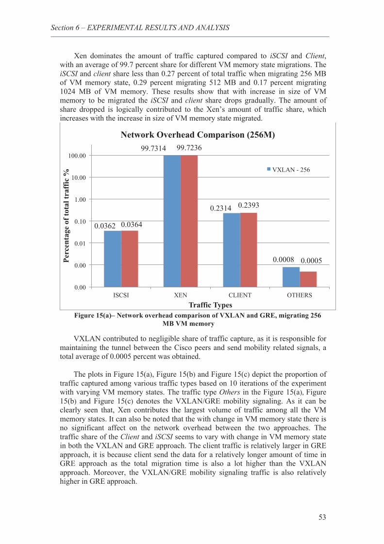
Section 6 – EXPERIMENTAL RESULTS AND ANALYSIS
53
Xen dominates the amount of traffic captured compared to iSCSI and Client,
with an average of 99.7 percent share for different VM memory state migrations. The iSCSI and client share less than 0.27 percent of total traffic when migrating 256 MB of VM memory state, 0.29 percent migrating 512 MB and 0.17 percent migrating 1024 MB of VM memory. These results show that with increase in size of VM memory to be migrated the iSCSI and client share drops gradually. The amount of share dropped is logically contributed to the Xen’s amount of traffic share, which increases with the increase in size of VM memory state migrated.
Figure 15(a)– Network overhead comparison of VXLAN and GRE, migrating 256
MB VM memory
VXLAN contributed to negligible share of traffic capture, as it is responsible for maintaining the tunnel between the Cisco peers and send mobility related signals, a total average of 0.0005 percent was obtained.
The plots in Figure 15(a), Figure 15(b) and Figure 15(c) depict the proportion of
traffic captured among various traffic types based on 10 iterations of the experiment with varying VM memory states. The traffic type Others in the Figure 15(a), Figure 15(b) and Figure 15(c) denotes the VXLAN/GRE mobility signaling. As it can be clearly seen that, Xen contributes the largest volume of traffic among all the VM memory states. It can also be noted that the with change in VM memory state there is no significant affect on the network overhead between the two approaches. The traffic share of the Client and iSCSI seems to vary with change in VM memory state in both the VXLAN and GRE approach. The client traffic is relatively larger in GRE approach, it is because client send the data for a relatively longer amount of time in GRE approach as the total migration time is also a lot higher than the VXLAN approach. Moreover, the VXLAN/GRE mobility signaling traffic is also relatively higher in GRE approach.
0.0362
99.7314
0.2314
0.0008
0.0364
99.7236
0.2393
0.0005
0.00
0.00
0.01
0.10
1.00
10.00
100.00
ISCSI XEN CLIENT OTHERS
Perc
enta
ge o
f tot
al tr
affic
%
Traffic Types
Network Overhead Comparison (256M)
VXLAN - 256
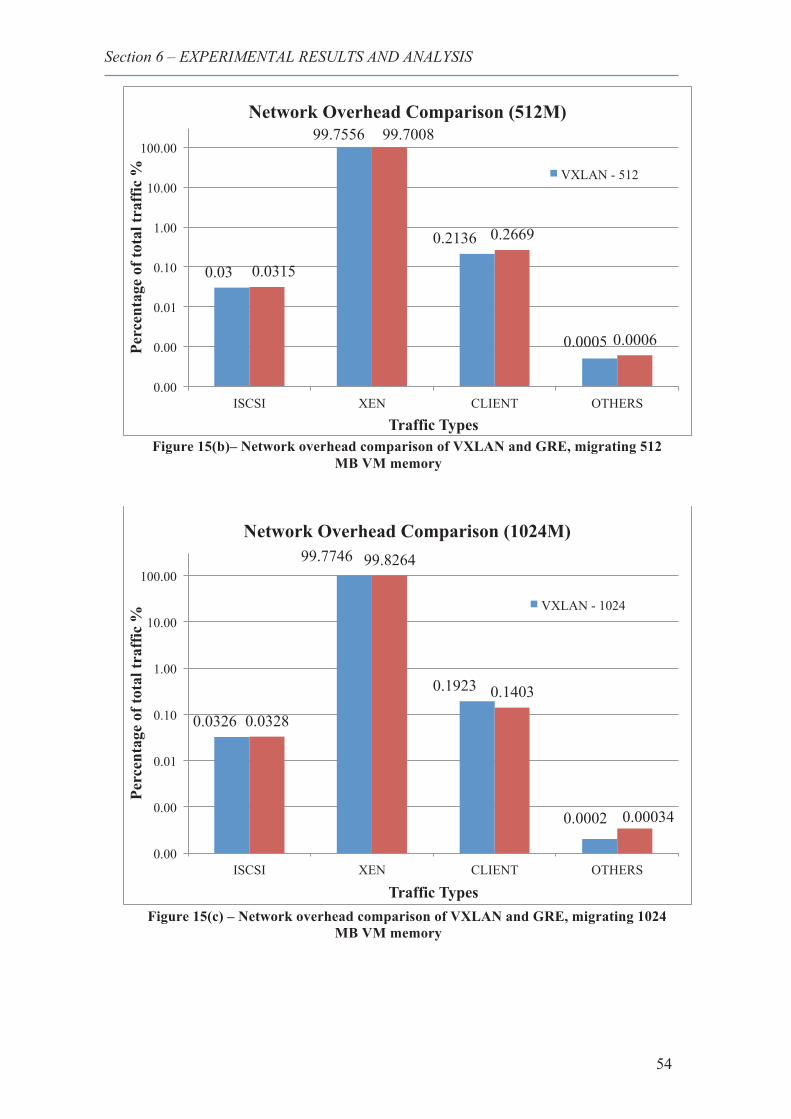
Section 6 – EXPERIMENTAL RESULTS AND ANALYSIS
54
Figure 15(b)– Network overhead comparison of VXLAN and GRE, migrating 512
MB VM memory
Figure 15(c) – Network overhead comparison of VXLAN and GRE, migrating 1024
MB VM memory
0.03
99.7556
0.2136
0.0005
0.0315
99.7008
0.2669
0.0006
0.00
0.00
0.01
0.10
1.00
10.00
100.00
ISCSI XEN CLIENT OTHERS
Perc
enta
ge o
f tot
al tr
affic
%
Traffic Types
Network Overhead Comparison (512M)
VXLAN - 512
0.0326
99.7746
0.1923
0.0002
0.0328
99.8264
0.1403
0.00034
0.00
0.00
0.01
0.10
1.00
10.00
100.00
ISCSI XEN CLIENT OTHERS
Perc
enta
ge o
f tot
al tr
affic
%
Traffic Types
Network Overhead Comparison (1024M)
VXLAN - 1024
55
7 Conclusion and Future Work This section summarizes our study based on the results and analysis done
implementing the VXLAN and GRE approaches. Relevant future work is also suggested for further research using the presented solutions.
7.1 Conclusion We have implemented the VXLAN and GRE approach to perform live VM
migration over WAN and maintained the network connectivity between the client and the VM during and after the migration process across the WAN. Open vSwitch was installed and configured on the hosts to allow VXLAN tunneling between the source host and destination, which provides the mobility support for migrating VMs between different subnets.
Experimental results from the laboratory test bed showed that the VXLAN
approach performs the VM migration relatively faster then the GRE approach along with minimal downtime. Moreover, we have observed that the signaling overhead caused by the VXLAN and GRE was negligible compared to other traffic generated during the migration process. VM migrations conducted with variable delays and variable for downtime showed a linear relationship. The downtime and total migration time increase gradually with increase in network delay. Though, the total migration time showed a strong relationship with variable VM memory state migration. The total migration time was double when migrating double the VM memory state. The established TCP connection session was maintained throughout the migration process for all the cases of variable delay and variable VM memory states. Thus, the TCP connection survived for multiple iterations of VM migration.
In general, our experimental test bed results suggest that VXLAN approach is
more refined and performed relatively better than the GRE approach with minimal downtime of 430 milliseconds and a minimal total migration time of approximately 25 seconds. Data centers in multitenant environment, Enterprises and Cloud providers may benefit from using these solutions for live VM migration.
7.2 Suggested Future work We have tested the approaches towards live migration using Xen hypervisor,
being a popular open source hypervisor, which supports Paravirtualization. Firstly, it would be interesting to perform the migration using KVM, another well-known hypervisor using hardware virtualization to observe how it performs using our approaches.
Secondly, we have performed live migration using the pre-copy technique
without introducing stress on the VM as the VM migration failed multiple times with our available hardware resources. It would be interesting to use the post-copy technique with induced stress on the VM to perform migrations, which suspends the VM on source and then migrates the VM onto the destination.
Thirdly, we have used a shared storage iSCSI for storing the disk state of the
VM. We have performed migrations, migrating the CPU, memory and network state of the VM. Disk state migration would be another interesting research, which can be done using our approaches towards live migration.
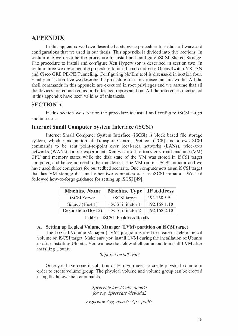
56
APPENDIX In this appendix we have described a stepwise procedure to install software and
configurations that we used in our thesis. This appendix is divided into five sections. In section one we describe the procedure to install and configure iSCSI Shared Storage. The procedure to install and configure Xen Hypervisor is described in section two. In section three we described the procedure to install and configure OpenvSwitch-VXLAN and Cisco GRE PE-PE Tunneling. Configuring NetEm tool is discussed in section four. Finally in section five we describe the procedure for some miscellaneous works. All the shell commands in this appendix are executed in root privileges and we assume that all the devices are connected as in the testbed representation. All the references mentioned in this appendix have been valid as of this thesis.
SECTION A In this section we describe the procedure to install and configure iSCSI target
and initiator.
Internet Small Computer System Interface (iSCSI) Internet Small Computer System Interface (iSCSI) is block based file storage
system, which runs on top of Transport Control Protocol (TCP) and allows SCSI commands to be sent point-to-point over local-area networks (LANs), wide-area networks (WANs). In our experiment, Xen was used to transfer virtual machine (VM) CPU and memory states while the disk state of the VM was stored in iSCSI target computer, and hence no need to be transferred. The VM run on iSCSI initiator and we have used three computers for our tedbed scenario. One computer acts as an iSCSI target that has VM storage disk and other two computers acts as iSCSI initiators. We had followed how-to-forge guidance for setting up iSCSI [49].
Machine Name Machine Type IP Address
iSCSI Server iSCSI target 192.168.5.5 Source (Host 1) iSCSI initiator 1 192.168.1.10
Destination (Host 2) iSCSI initiator 2 192.168.2.10 Table a – iSCSI IP address Details
A. Setting up Logical Volume Manager (LVM) partition on iSCSI target The Logical Volume Manager (LVM) program is used to create or delete logical
volume on iSCSI target. Make sure you install LVM during the installation of Ubuntu or after installing Ubuntu. You can use the below shell command to install LVM after installing Ubuntu.
$apt-get install lvm2
Once you have done installation of lvm, you need to create physical volume in order to create volume group. The physical volume and volume group can be created using the below shell commands.
$pvcreate /dev/<sda_name> for e.g. $pvcreate /dev/sda2
$vgcreate <vg_name> <pv_path>
57
for e.g. $vgcreate vg0 /dev/sda2
The next step is to create logical volume to store virtual machine disks. You can use the below shell command to create a logical volume of 40 gigabytes of volume name “shared” in volume group “vg0”.
$lvcreate –n <volume_name> -L <size in G or M> <volume group>
for e.g. $lvcreate –n shared –L 40G vg0
B. Installing and Configuring iSCSI target The iSCSI target provides a shared storage for Host 1 (Source) and Host 2
(Destination). The VM running on the iSCSI initiator while the VM disk is stored on the iSCSI target. We have installed iSCSI target program on Ubuntu 14.04.1 LTS operating system. You can use the below shell command in Ubuntu terminal to install iSCSI target.
$aptitude install iscsitarget iscsitarget-modules-`uname –r`
Once you have done the installation, the iscsitarget file located at /etc/default/
should be opened and set the “ISCSITARGET_ENABLE = true” will enable iSCSI target when Ubuntu boot.
Then next, open the file “gedit /etc/iet/ietd.conf” and add the following lines by
commenting all the existed content.
Target iqn.2015-02.com.example:shared.lun1 IncomingUser OutgoingUser Lun 0 Path=/dev/vg0/shared,Type=fileio Alias LUN1
The target name should be a unique name according to the name defined by the
iSCSI standard. Target iqn. <yyyy-mm> . <reserved domain name> [:<identifier>] is the iSCSI defined standard naming. The username and password can be added for authenticating the iSCSI initiators (Host 1 and Host 2). The line starting with Lun 0 indicated the path of the shared storage.
By adding the ip address of the initiators to the file “gedit
/etc/iet/initiators.allow” the target will allow only those hosts to be connected to it.
Iqn.2015-02.com.example:shared.lun1 192.168.1.10, 192.168.2.10
The entire network pool can be selected by adding the network address like below to the file initiators.allow.
iqn.2015-02.com.example:shared.lun1 192.168.1.0/24, 192.168.2.0/24
After saving the modified file, the iSCSI target service should be restarted.
$/etc/init.d/iscsitarget start
58
C. Installing and Configuring iSCSI initiator
We are having two iSCSI initiators (Host 1 and Host 2). So, you can use the below shell command to install iSCSI initiator on two hosts.
$aptitude install open-iscsi
Once you have done the installation, the iscsi initiator file “gedit
/etc/iscsi/iscsid.conf” should be opened and set the “node.startup = automatic” will allow initiator to automatically connect to iSCSI target.
After saving the modified file, the iSCSI initiator service should be restarted.
$/etc/init.d/open-iscsi start
Next, the iSCSI target can be discovered by using the below shell command.
$iscsiadm –m discovery –t st –p 192.168.5.5
Finally, the iSCSI initiator can be login into the iSCSI target by using the below shell command.
Iscsiadm –m node –login
SECTION B In this section we describe the procedure to install and configure Xen Hypervisor
and VM creation.
Xen Hypervisor Installation We have followed the Xen Community help document [50] to install Xen
hypervisor. We have installed 64-bit Xen Hypervisor Xen 4.4 on Ubuntu 14.04.1 LTS 64-bit operating system. The 64-bit hypervisor works with a 32-bit dom0 kernel and even allows you to run both 32-bit and 64-bit guest operating system. You can use the below shell command to install Xen hypervisor.
$apt-get install xen-hypervisor-amd64
Next, as of Ubuntu 14.04, grub will automatically choose Xen first to boot if Xen
is installed and the “xl” as default Xen tool stack. If you’re running an earlier version of Ubuntu 14.04, you have to modify the
grub to make Xen default on boot and make “xm” as default tool stack. The below shell command can be used to set Xen boot default.
$sed –I ‘s/GRUB_DEFAULT=.*\+/GRUB_DEFAULT=”Xen 4.1-amd64”/’
/etc/default/grub
Then now make xm as default Xen tool stack.
$sed –I ‘s/TOOLSTACK=.*\+/TOOLSTACK=”xm”/’ /etc/default/xen
59
Now reboot the system so that the system boots with Xen hypervisor. After restart you can verify the Xen installation has succeeded by typing “xl list” in the terminal, which displays Domain-0 as result.
$reboot $xl list
A. Network Configuration
We have emulated the network link between physical host and virtual machine using Linux Bridge. The Linux Bridge can be installed using the below shell command.
$apt-get install bridge-utils
Next, open the file “gedit /etc/network/interfaces” and modify it as below. You
can replace manual by static with proper ip address, netmask and gateway.
Auto lo iface lo net loopback auto br0 iface br0 net manual bridge_ports eth0 auto eth0 iface eth0 net manual
Restart the networking service to make the changes effective.
$/etc/init.d/networking restart or $service networking restart
N.B: You can also use the synaptic package manager to install Xen hypervisor
and Network Bridge [51].
B. Configuring Xen to allow VM Migration Open the file “gedit /etc/xen/xend-config.sxp” and modify the file to have the
following lines, which enables live migration and allow virtual machine to migrate from one host to another over network [52].
(xend-relocation-server yes) (xend-relocation-port 8002) (xend-relocation-address ’’) (xend-relocation-hosts-allow ’’)
Now, you can restart the Xen to enable the changes. Be sure you run this command from the location “/etc/xen/”.
$service xen restart
60
C. Creating Virtual Machines Xen supports both hardware-assisted VM (HVM) and paravirtualized VM
(PVM). Depending on the hardware capability, you may create PVM or HVM. In our thesis we will describe how you can create a paravirtualized virtual machine. Installing xen-tools [53] package to create virtual machine automatically by using debootstrap. The below shell command is used to install xen-tools.
$apt-get install xen-tools
In our experiment, the VM ran Ubuntu 12.04 LTS OS. We used Ubuntu 14.04.1
LTS operating system, as it is reliable, stable and the latest fully developed Ubuntu distribution. In order to run the OpenvSwitch hotplug script, which supports from Xen 4.3 or later is another reason to choose this operating system [38]. However, the installed xen-tools package doesn’t include the distribution for precise. So, we download the xen-tools v4.4-1 and using the below shell commands we updated to the current version.
$wget http://se.archive.ubuntu.com/ubuntu/pool/universe/x/xen-tools/xen-tools_4.4-
1_all.deb
$dpkg –I xen-tools_4.4-1_all.deb
Now, you can create virtual machines in iSCSI-shared storage.
D. Installing VM in iSCSI-shared storage The VM disk is stored in iSCSI and can be created using below shell command.
$xen-create-image –dhcp –hostname sample –memory 256M –lvm vg0 –bridge br1 –
pygrub –dist precise –passwd
In the above command, “sample” is the name of the VM, “vg0” is the name of the volume group of iSCSI. For additional information on xen-create-image, you can look into the man page. After completion of VM creation, open the VM configuration file “/etc/xen/sample.cfg” and you can modify the vCPU, memory and relative fields. Then SSH the configuration file to the destination host where the VM will be migrated. The configuration file looks like the following text.
Bootloader = ‘/usr/lib/xen-default/bin/pygrub’ vcpu = ‘1’ memory = ‘256’ root = ‘/dev/xvda2 ro’ disk = [‘phy:/dev/vg0/sample-disk,xvda2,w’,’ phy:/dev/vg0/sample-swap,xvda1,w’] name = ‘sample’ dhcp = ‘dhcp’ vif = [‘mac=00:16:3E:C4:24:01,bridge=br1’] on_poweroff = ‘destroy’ on_reboot = ‘restart’ on_crash = ‘restart’
61
SECTION C In this section we describe the procedure to install and configure OpenvSwitch-
VXLAN and configuration of Cisco GRE PE-PE Tunneling.
Installing and Configuring OpenvSwitch (OVS) OpenvSwitch supports in forwarding traffic between different VMs on the same
physical network and also forwards traffic between the physical network and VM. We following the guidance from the document INSTALL file for setting up OVS [54]. You can start with installing the dependencies before building the latest OVS. You can install the dependencies by using the below shell command.
$apt-get install python-simplejson python-qt4 python-twisted-conch automake autoconf
gcc uml-utilities libtool build-essential git pkg-config linux-headers-`uname –r`
In our thesis experiment we have used OVS version 2.3.0, as it is the latest stable release from OpenvSwitch organization, which is also LTS (Long-Term Support). Now, you can download the OVS v2.3.0 tar file and extract the file by using the below shell commands.
$wget http://openvswitch.org/releases/openvswitch-2.3.0.tar.gz
$tar zxvf openvswitch-2.3.0.tar.gz
After extracting the file, you need to change the current directory to OVS file
before compiling OpenvSwitch from source. The following shell commands are used to compile OVS.
$./boot.sh $./configure –with-linux=/lib/modules/`uname –r`/build $make && make install $make modules_install $modprobe openvswitch $insmod datapath/linux/openvswitch.ko
Now, you can initialize the OpenvSwitch configuration database using the
ovsdb-tool. The below shell commands are used to initialize the configuration file.
$touch /usr/local/etc/ovs-vswitchd.conf $mkdir –p /usr/local/etc/openvswitch $ovsdb-tool create /usr/local/etc/openvswitch/conf.db vswitchd/vswitch.ovsschema
Next, before starting up ovs-vswitchd itself, you need to start the OVS
configuration database, ovsdb-server. By starting ovsdb-server, the configuration is stored into a file that is persistent even after restart. The below shell command is used for starting ovsdb-server.
$ovsdb-server –remote=punix:/usr/local/var/run/openvswitch/db.sock –remote=db:Open_vSwitch,Open_vSwitch,manager_options –pidfile –detach –log-file
62
Then you need to initialize the database using ovs-vsctl and it is only necessary for the first time installation. After that you can start the OpenvSwitch by using the below shell commands.
$ovs-vsctl –no-wait init $ovs-vswitchd –pidfile –detach –log-file
Now, you can use the below shell commands to verify that the modules have
been loaded or not and also the output of OVS.
$lsmod | grep openvswitch $ovs-vsctl show $ovs-vsctl –version
Now, you can set up bridges and other OpenvSwitch features using ovs-vsctl.
N.B: You can also put all the above text into a bash file and give it execute
permissions with “chmod +x filename” and run it.
A. Configuring Linux Networking and VXLAN Tunnel on OVS Each system which participating in the network will be required a virtual bridge.
The following shell commands are used to configure bridges on OVS and setting up VXLAN tunnel.
$ovs-vsctl add-br br0 $ovs-vsctl add-br br1 $ovs-vsctl add-port br0 eth0 $ifconfig eth0 0 && ifconfig br0 192.168.1.10 netmask 255.255.255.0 $ifconfig br1 IP netmask 255.255.255.0 $ovs-vsctl add-port br1 vx1 –set interface vx1 type=vxlan options:remote_ip=192.168.2.10 options:key=flow
In the above commands, “br0” and “br1” are the virtual bridges added to OVS.
The physical interface “eth0” is attached to ”br0” so now “br0” is the default gateway NIC instead of “eth0” since it is the bridge interface of “br0”.
In the last command, “vx1” is the port name of the “br1” bridge and
“type=vxlan” is used to set up vxlan tunneling between Source (Host 1) and Destination (Host 2). And the “key=flow” is the option to set VNI (VXLAN Network Identifier) for the tunnel, if the option is not specified VNI=0 will be used for the tunneling. If you need more than one virtual network’s over a single vxlan tunnel then you need to specify VNI to separate the traffic between the virtual networks.
N.B: You need to run the same above commands in Host 1 (Source) and Host 2
(Destination) systems. The only change will be the IP address in “br0”, “br1” and “remote_ip” between the two systems. The “key” will be remaining same in OpenvSwitch of both systems.
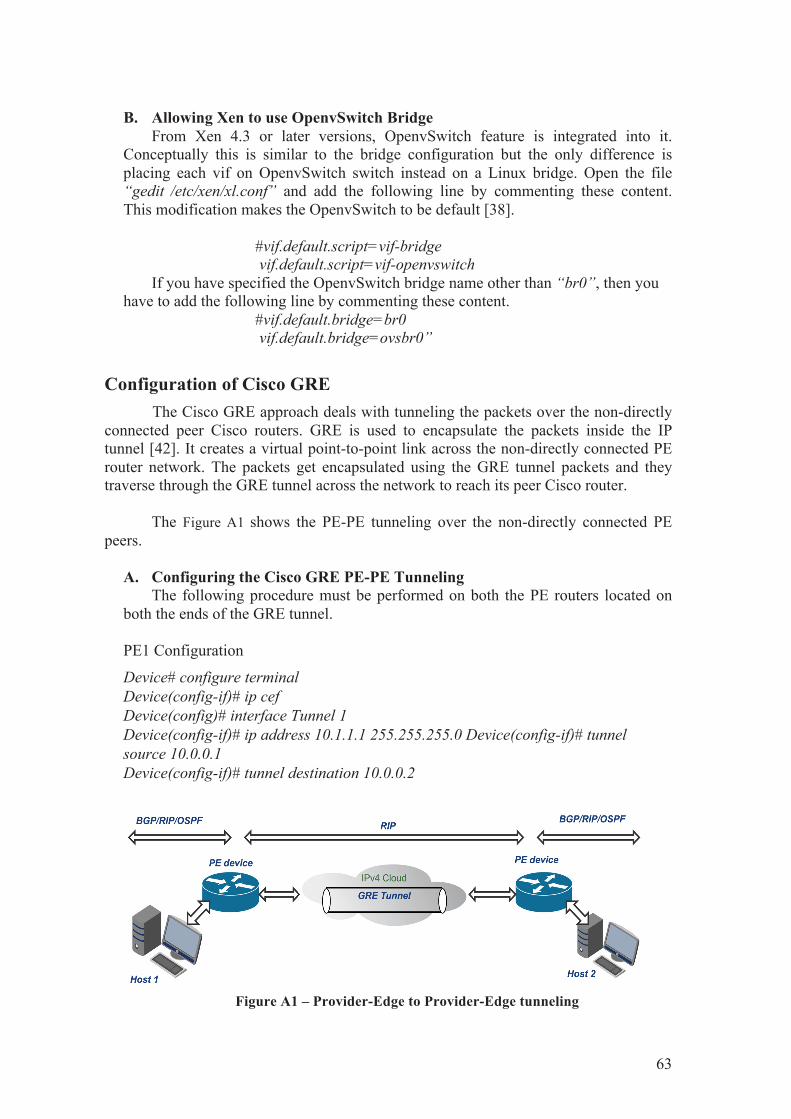
63
B. Allowing Xen to use OpenvSwitch Bridge
From Xen 4.3 or later versions, OpenvSwitch feature is integrated into it. Conceptually this is similar to the bridge configuration but the only difference is placing each vif on OpenvSwitch switch instead on a Linux bridge. Open the file “gedit /etc/xen/xl.conf” and add the following line by commenting these content. This modification makes the OpenvSwitch to be default [38].
#vif.default.script=vif-bridge vif.default.script=vif-openvswitch
If you have specified the OpenvSwitch bridge name other than “br0”, then you have to add the following line by commenting these content.
#vif.default.bridge=br0 vif.default.bridge=ovsbr0”
Configuration of Cisco GRE The Cisco GRE approach deals with tunneling the packets over the non-directly
connected peer Cisco routers. GRE is used to encapsulate the packets inside the IP tunnel [42]. It creates a virtual point-to-point link across the non-directly connected PE router network. The packets get encapsulated using the GRE tunnel packets and they traverse through the GRE tunnel across the network to reach its peer Cisco router.
The Figure A1 shows the PE-PE tunneling over the non-directly connected PE
peers.
A. Configuring the Cisco GRE PE-PE Tunneling The following procedure must be performed on both the PE routers located on
both the ends of the GRE tunnel.
PE1 Configuration
Device# configure terminal Device(config-if)# ip cef Device(config)# interface Tunnel 1 Device(config-if)# ip address 10.1.1.1 255.255.255.0 Device(config-if)# tunnel source 10.0.0.1 Device(config-if)# tunnel destination 10.0.0.2
Figure A1 – Provider-Edge to Provider-Edge tunneling
64
PE2 Configuration
Device# configure terminal Device(config-if)# ip cef Device(config)# interface Tunnel 1 Device(config-if)# ip address 10.1.1.2 255.255.255.0 Device(config-if)# tunnel source 10.0.0.2 Device(config-if)# tunnel destination 10.0.0.1
B. Enable RIP
Routing Information Protocol is configured on both the Cisco routers for the routers to gain the information about the IP networks behind the PE routers. The routes are stored in the default routing table.
The following procedure shows the configuration of RIP on both the PE routers: PE1 Configuration Router(config)# router rip Router(config-router)# 192.168.1.0 PE2 Configuration Router(config)# router rip Router(config-router)# 192.168.2.0 By default, the protocol receives only sends RIP Version 1 packets but receives
RIP Version 1 and Version 2 packets.
SECTION D In this section we describe the procedure to configure NetEm.
Configuring NetEm NetEm is a Linux based tool used to add delay, packet loss and many other
characteristics to the outgoing packets. It is used to emulate the WAN properties by introducing network delay and jitter. Typically the network delay is not uniform in WAN, the delay variation can be describe by using pareto distribution in NetEm. The below shell command is used to introduce the Inter-Europe delay of 30 ms with a jitter of 6 ms which is pareto distributed. ”tc” allows us to specify the ”queueing discipline (qdisc)” used for sending and operating on outbound packets on an interface. And also ”qdisc” defines how the outbound packets are ordered and sent. The below command is applied at eth0 and eth1 interfaces of the Linux PC router.
$tc qdisc add dev eth0/eth1 root netem delay 30ms 6ms distribution pareto
65
SECTION E In this section we describe the procedure for some miscellaneous works.
Create NetEm Own Distribution table The NetEm emulator is widely used to emulate the network environment. In
NetEm, it is possible to create and use custom distribution tables to better approximate the round-trip-time variations in the network. This can done using the iproute2 source code for generating the own distribution table [55].
After downloading the source code, enter into the NetEm subdirectory and compile the maketable and stats utilities using the below shell command.
$gcc maketable.c –o maketable –lm
$gcc stats.c –o stats –lm Next, we need to have some delay statistics for emulating the WAN
environment. Consider you want to emulate the network between a server in Greece and a client PC in Sweden. Then run a ping between these 2 systems for long period of time, mostly a whole day is better and save the result in a text file.
Next, using the below shell command we will extract all the round-trip-time in a
new text file.
$cat old.txt | grep icmp_seq | cut –d’=’ –f4 | cut –d’ ‘ –f1 > new.txt Finally, we can create a distribution table using the maketable utility so that
NetEm can understand it. The below commands is used to create distribution table and copy the “.dist” file to “/usr/lib/tc” so that NetEm can find it.
$./maketable new.txt > owndist.dist
$cp owndist.dist /usr/lib/tc
Additionally, you can obtain the mean and standard deviation of the collected data using the stats utility in the source code. The below shell command is used to obtain the mean (mu), standard deviation (sigma) and correlation (rho) of the collected data.
$./stats new.txt
Finally, you can use NetEm to emulate the network between Sweden and Greece
by using the below shell command.
$tc qdisc add dev eth0 root netem mu sigma distribution owndist
Pareto Distribution We have implemented Pareto distribution in NetEm to emulate the WAN
scenario in our testbed. We ran multiple tests with variable values of delay and jitter to get a long heavy tail distribution. The variable delays are selected based on the regions around the globe, Trans-Atlantic (90 ms), Trans-Pacific (160 ms) and Intra-Europe (30 ms) [56]. The jitter values are selected based on multiple tests run using Pareto distribution in NetEm to obtain a long heavy tail plots.
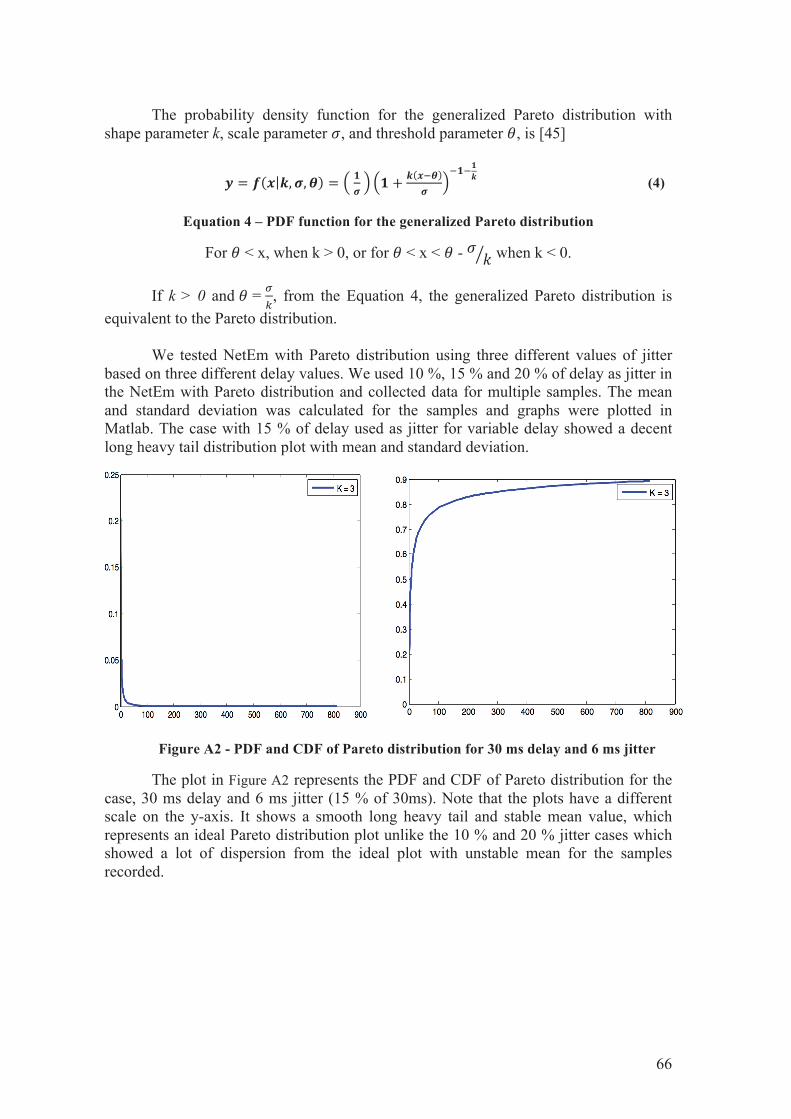
66
The probability density function for the generalized Pareto distribution with
shape parameter k, scale parameter , and threshold parameter , is [45]
(4)
Equation 4 – PDF function for the generalized Pareto distribution
For < x, when k > 0, or for < x < - when k < 0.
If k > 0 and = , from the Equation 4, the generalized Pareto distribution is equivalent to the Pareto distribution.
We tested NetEm with Pareto distribution using three different values of jitter
based on three different delay values. We used 10 %, 15 % and 20 % of delay as jitter in the NetEm with Pareto distribution and collected data for multiple samples. The mean and standard deviation was calculated for the samples and graphs were plotted in Matlab. The case with 15 % of delay used as jitter for variable delay showed a decent long heavy tail distribution plot with mean and standard deviation.
Figure A2 - PDF and CDF of Pareto distribution for 30 ms delay and 6 ms jitter
The plot in Figure A2 represents the PDF and CDF of Pareto distribution for the case, 30 ms delay and 6 ms jitter (15 % of 30ms). Note that the plots have a different scale on the y-axis. It shows a smooth long heavy tail and stable mean value, which represents an ideal Pareto distribution plot unlike the 10 % and 20 % jitter cases which showed a lot of dispersion from the ideal plot with unstable mean for the samples recorded.

67
68
BIBLIOGRAPHY
[1] T. Wood, K. K. Ramakrishnan, P. Shenoy, and J. van der Merwe, “CloudNet: Dynamic Pooling of Cloud Resources by Live WAN Migration of Virtual Machines,” in Proceedings of the 7th ACM SIGPLAN/SIGOPS International Conference on Virtual Execution Environments, New York, NY, USA, 2011, pp. 121–132.
[2] “The Advantages of Using Virtualization Technology in the Enterprise,” White Paper, Vmware Inc., Palo Alto, CA, USA, 2007. [Online]. Available: https://software.intel.com/en-us/articles/the-advantages-of-using-virtualization-technology-in-the-enterprise. [Accessed: 18-May-2014].
[3] “Understanding Full Virtualization, Paravirtualization, and Hardware Assist,” White Paper, Vmware Inc., Palo Alto, CA, USA, 2007. .
[4] C. Clark, K. Fraser, S. Hand, J. G. Hansen, E. Jul, C. Limpach, I. Pratt, and A. Warfield, “Live Migration of Virtual Machines,” in Proceedings of the 2Nd Conference on Symposium on Networked Systems Design & Implementation – Volume 2, Berkeley, CA, USA, 2005, pp. 273–286.
[5] R. Bradford, E. Kotsovinos, A. Feldmann, and H. Schiöberg, “Live Wide-area Migration of Virtual Machines Including Local Persistent State,” in Proceedings of the 3rd International Conference on Virtual Execution Environments, New York, NY, USA, 2007, pp. 169–179.
[6] L. Zhang, D. Meyer, and K. Fall, “Report from the IAB Workshop on Routing and Addressing.” [Online]. Available: http://tools.ietf.org/html/rfc4984. [Accessed: 02-Sep-2014].
[7] K. Takahashi, K. Sasada, and T. Hirofuchi, “A Fast Virtual Machine Storage Migration Technique Using Data Deduplication,” presented at the CLOUD COMPUTING 2012, The Third International Conference on Cloud Computing, GRIDs, and Virtualization, 2012, pp. 57–64.
[8] “draft-mahalingam-dutt-dcops-vxlan-09.” [Online]. Available: https://datatracker.ietf.org/doc/draft-mahalingam-dutt-dcops-vxlan/. [Accessed: 22-May-2014].
[9] “VXLAN Overlay Networks: Enabling Network Scalability for a Cloud Infrastructure,” Emulex White Paper. .
[10] “Xen Project Software Overview - Xen.” [Online]. Available: http://wiki.xen.org/wiki/Xen_Project_Software_Overview. [Accessed: 18-May-2014].
[11] C. Graziano, “A performance analysis of Xen and KVM hypervisors for hosting the Xen Worlds Project,” Graduate Theses and Dissertations, Jan. 2011.
[12] A. Singh, “An Introduction to Virtualization.” [Online]. Available: http://www.kernelthread.com/publications/virtualization/. [Accessed: 26-Nov-2014].
[13] J. Watson, “VirtualBox: Bits and Bytes Masquerading As Machines,” Linux J., vol. 2008, no. 166, Feb. 2008.
[14] “Virtualization Spectrum - Xen.” [Online]. Available: http://wiki.xen.org/wiki/Virtualization_Spectrum. [Accessed: 26-Nov-2014].
[15] P. Barham, B. Dragovic, K. Fraser, S. Hand, T. Harris, A. Ho, R. Neugebauer, I. Pratt, and A. Warfield, “Xen and the Art of Virtualization,” in Proceedings of the Nineteenth ACM Symposium on Operating Systems Principles, New York, NY, USA, 2003, pp. 164–177.
[16] S. Azodolmolky, R. Nejabati, S. Peng, A. Hammad, M. P. Channegowda, N. Efstathiou, A. Autenrieth, P. Kaczmarek, and D. Simeonidou, “Optical FlowVisor: an OpenFlow-based optical network virtualization approach,” in National Fiber Optic Engineers Conference, 2012, p. JTh2A–41.
[17] S. Kassahun, A. Demessie, and D. Ilie, “A PMIPv6 approach to maintain network connectivity during VM live migration over the internet,” in 2014 IEEE 3rd International Conference on Cloud Networking (CloudNet), 2014, pp. 64–69.
[18] S. Sreekanth, “VMware vSphere 5.1 vMotion Architecture, Performance and Best Practices,” White Paper, VMware Inc., Palo Alto, CA, USA, 2012. .
[19] W. R. Stevens, TCP/IP Illustrated. Addison-Wesley, 1994. . [20] D. S. Milo’jičić, F. Douglis, Y. Paindaveine, R. Wheeler, and S. Zhou, “Process Migration,”
ACM Comput. Surv., vol. 32, no. 3, pp. 241–299, Sep. 2000. [21] A. Mashtizadeh, E. Celebi, T. Garfinkel, and M. Cai, “The design and evolution of live storage
migration in VMware ESX,” in in Proceedings of the 2011 USENIX conference on USENIX annual technical conference, 2011, pp. 14–14.
[22] Y. Luo, B. Zhang, X. Wang, Z. Wang, Y. Sun, and H. Chen, “Live and incremental whole-system migration of virtual machines using block-bitmap,” in Proceedings - IEEE International Conference on Cluster Computing, ICCC, 2008, pp. 99–106.
[23] S. Akoush, R. Sohan, B. Roman, A. Rice, and A. Hopper, “Activity based sector synchronisation: Efficient transfer of disk-state for WAN live migration,” in IEEE International Workshop on
69
Modeling, Analysis, and Simulation of Computer and Telecommunication Systems - Proceedings, 2011, pp. 22–31.
[24] P. Reisner and L. Ellenberg, “Replicated storage with shared disk semantics,” in Proceedings of the 12th International Linux System Technology Conference (Linux- Kongress), Germany, 2005, pp. 111–119.
[25] F. Haas, P. Reisner, and L. Ellenberg, “The DRBD user’s guide,” LINBIT HA Solutions GmbH, 2011.
[26] M. G. Marsh, Policy Routing Using Linux. Indianapolis, IN, USA: Sams, 2001. [27] F. Travostino, P. Daspit, L. Gommans, C. Jog, C. de Laat, J. Mambretti, I. Monga, B. van
Oudenaarde, S. Raghunath, and P. Yonghui Wang, “Seamless live migration of virtual machines over the MAN/WAN,” Future Generation Computer Systems, vol. 22, no. 8, pp. 901–907, Oct. 2006.
[28] E. Harney, S. Goasguen, J. Martin, M. Murphy, and M. Westall, “The Efficacy of Live Virtual Machine Migrations Over the Internet,” in 2007 Second International Workshop on Virtualization Technology in Distributed Computing (VTDC), 2007, pp. 1–7.
[29] J. Van der Merwe, A. Cepleanu, K. D’Souza, B. Freeman, A. Greenberg, D. Knight, R. McMillan, D. Moloney, J. Mulligan, H. Nguyen, M. Nguyen, A. Ramarajan, S. Saad, M. Satterlee, T. Spencer, D. Toll, and S. Zelingher, “Dynamic Connectivity Management with an Intelligent Route Service Control Point,” in Proceedings of the 2006 SIGCOMM Workshop on Internet Network Management, New York, NY, USA, 2006, pp. 29–34.
[30] R. Kawashima and H. Matsuo, “Performance Evaluation of Non-tunneling Edge-Overlay Model on 40GbE Environment,” in 2014 IEEE 3rd Symposium on Network Cloud Computing and Applications (NCCA), 2014, pp. 68–74.
[31] Morton, A., Raisanen, V. and Grotefeld, G. “Network performance measurement with periodic streams,” RFC 3432, Nov. 2002.
[32] “VXLAN Overview: Cisco,” Cisco. [33] B. Pfaff, J. Pettit, K. Amidon, M. Casado, T. Koponen, and S. Shenker, “Extending Networking
into the Virtualization Layer.,” in Hotnets, 2009. [34] S. Hanks, D. Meyer, D. Farinacci, and P. Traina, “Generic Routing Encapsulation (GRE).”
[Online]. Available: http://tools.ietf.org/html/rfc2784. [Accessed: 03-Dec-2014]. [35] R. Davoli, “VDE: virtual distributed Ethernet,” in First International Conference on Testbeds
and Research Infrastructures for the Development of Networks and Communities, 2005. Tridentcom 2005, 2005, pp. 213–220.
[36] P. Barham, B. Dragovic, K. Fraser, S. Hand, T. Harris, A. Ho, R. Neugebauer, I. Pratt, and A. Warfield, “Xen and the Art of Virtualization,” in Proceedings of the Nineteenth ACM Symposium on Operating Systems Principles, New York, NY, USA, 2003, pp. 164–177.
[37] A. Jurgelionis, J. Laulajainen, M. Hirvonen, and A. I. Wang, “An Empirical Study of NetEm Network Emulation Functionalities,” in 2011 Proceedings of 20th International Conference on Computer Communications and Networks (ICCCN), 2011, pp. 1–6.
[38] “Xen Networking - Xen.” [Online]. Available: http://wiki.xenproject.org/wiki/Xen_Networking. [Accessed: 05-Jan-2015].
[39] “netem | The Linux Foundation.” [Online]. Available: http://www.linuxfoundation.org/collaborate/workgroups/networking/netem. [Accessed: 05-Mar-2015].
[40] “Generic Routing Encapsulation (GRE),” Cisco. [Online]. Available: http://cisco.com/c/en/us/tech/ip/generic-routing-encapsulation-gre/index.html. [Accessed: 03-Mar-2015].
[41] S. Hanks, D. Meyer, D. Farinacci, and P. Traina, “Generic Routing Encapsulation (GRE).” [Online]. Available: http://tools.ietf.org/html/rfc2784. [Accessed: 03-Mar-2015].
[42] “MPLS: Layer 3 VPNs Configuration Guide, Cisco IOS XE Release 3S - MPLS over GRE [Support],” Cisco. [Online]. Available: http://cisco.com/c/en/us/td/docs/ios-xml/ios/mp_l3_vpns/configuration/xe-3s/mp-l3-vpns-xe-3s-book/mp-vpn-gre.html. [Accessed: 03-Mar-2015].
[43] “The Pareto Distribution”: http://www.math.uah.edu/stat/special/Pareto.html. Accessed: 2015-03-22.
[44] “Pareto distribution,” Wikipedia, the free encyclopedia. 19-Jan-2015. [45] “Generalized Pareto Distribution - MATLAB & Simulink - MathWorks Nordic”:
http://se.mathworks.com/help/stats/generalized-pareto-distribution.html. Accessed: 2015-03-22. [46] Bolotin, V.A. 1994. “Modeling call holding time distributions for CCS network design and
performance analysis”, IEEE Journal on Selected Areas in Communications. 12, 3 (Apr. 1994), 433–438.
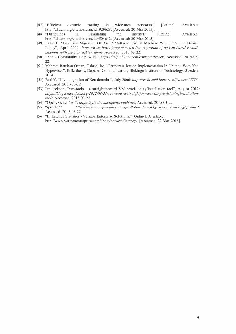
70
[47] “Efficient dynamic routing in wide-area networks.” [Online]. Available: http://dl.acm.org/citation.cfm?id=929623. [Accessed: 20-Mar-2015].
[48] “Difficulties in simulating the internet.” [Online]. Available: http://dl.acm.org/citation.cfm?id=504642. [Accessed: 20-Mar-2015].
[49] Falko.T, “Xen Live Migration Of An LVM-Based Virtual Machine With iSCSI On Debian Lenny”, April 2009: https://www.howtoforge.com/xen-live-migration-of-an-lvm-based-virtual-machine-with-iscsi-on-debian-lenny. Accessed: 2015-03-22.
[50] “Xen - Community Help Wiki”: https://help.ubuntu.com/community/Xen. Accessed: 2015-03-22.
[51] Mehmet Batuhan Özcan, Gabriel Iro, “Paravirtualization Implementation In Ubuntu With Xen Hypervisor”, B.Sc thesis, Dept. of Communication, Blekinge Institute of Technology, Sweden, 2014.
[52] Paul.V, “Live migration of Xen domains”, July 2006: http://archive09.linux.com/feature/55773. Accessed: 2015-03-22.
[53] Ian Jackson, “xen-tools – a straightforward VM provisioning/installation tool”, August 2012: https://blog.xenproject.org/2012/08/31/xen-tools-a-straightforward-vm-provisioninginstallation-tool/. Accessed: 2015-03-22.
[54] “OpenvSwitch/ovs”: https://github.com/openvswitch/ovs. Accessed: 2015-03-22. [55] “iproute2”: http://www.linuxfoundation.org/collaborate/workgroups/networking/iproute2.
Accessed: 2015-03-22. [56] “IP Latency Statistics - Verizon Enterprise Solutions.” [Online]. Available:
http://www.verizonenterprise.com/about/network/latency/. [Accessed: 22-Mar-2015].


![ShuttleDB: Database-Aware Elasticity in the Cloud · cloud elasticity mechanisms such as VM migration or VM replication (e.g., Amazon’s auto-scaling [2]), the approach does not](https://img.pdfslide.us/doc/110x75/5f0b23ee7e708231d42f0c4f/shuttledb-database-aware-elasticity-in-the-cloud-cloud-elasticity-mechanisms-such.jpg)