A Performance Monitoring Approach for the Novel Lillgrund

6636 IEEE TRANSACTIONS ON INDUSTRIAL ELECTRONICS, VOL. 62, NO. 10, OCTOBER 2015

A Performance Monitoring Approach for theNovel Lillgrund Offshore Wind Farm

Evangelos Papatheou, Nikolaos Dervilis, Andrew Eoghan Maguire,Ifigeneia Antoniadou, and Keith Worden

Abstract—The use of offshore wind farms has beengrowing in recent years. Europe is presenting a geomet-rically growing interest in exploring and investing in suchoffshore power plants as the continent’s water sites offerimpressive wind conditions. Moreover, as human activitiestend to complicate the construction of land wind farms,offshore locations, which can be found more easily neardensely populated areas, can be seen as an attractivechoice. However, the cost of an offshore wind farm is rel-atively high, and therefore, their reliability is crucial if theyever need to be fully integrated into the energy arena. Thispaper presents an analysis of supervisory control and dataacquisition (SCADA) extracts from the Lillgrund offshorewind farm for the purposes of monitoring. An advanced androbust machine-learning approach is applied, in order toproduce individual and population-based power curves andthen predict measurements of the power produced fromeach wind turbine (WT) from the measurements of the otherWTs in the farm. Control charts with robust thresholdscalculated from extreme value statistics are successfullyapplied for the monitoring of the turbines.

Index Terms—Machine learning, offshore wind farm, pat-tern recognition, supervisory control and data acquisition(SCADA), wind turbine (WT) monitoring.

I. INTRODUCTION

THE idea of using supervisory control and data acquisition(SCADA) measurements for structural health monitoring

(SHM) and condition monitoring has received attention fromboth the wind energy and structural engineering communities,particularly for the monitoring of critical infrastructures [1]. Inorder to maintain a qualitative profit with large offshore windfarms, a major challenge is to keep operational and maintenancecosts to the lowest level by ensuring reliable and robust moni-toring systems. For this reason, data mining and machine learn-ing are promising approaches for modeling wind energy aspects

Manuscript received October 3, 2014; revised January 22, 2015 andApril 2, 2015; accepted April 30, 2015. Date of publication June 5, 2015;date of current version September 9, 2015. This work was supported bythe U.K. Engineering and Physical Sciences Research Council (EPSRC)under Grant EP/J016942/1 and Grant EP/K003836/2.

E. Papatheou, N. Dervilis, I. Antoniadou, and K. Worden are withthe Dynamics Research Group, Department of Mechanical Engineer-ing, The University of Sheffield, Sheffield, S1 3JD, U.K. (e-mail:[email protected]).

A. E. Maguire is with Vattenfall Research and Development, NewRenewables, Edinburgh, EH8 8AE, U.K.

Color versions of one or more of the figures in this paper are availableonline at http://ieeexplore.ieee.org.

Digital Object Identifier 10.1109/TIE.2015.2442212

such as power prediction or wind load forecasting. It is perhapswell known that there has been a recent expansion in the useof wind energy, which is likely to continue with an acceleratedpace over the coming years. Among the various forms of windenergy, offshore wind farms have become more popular, mainlydue to the broader choice regarding their location and also thegenerally steadier and higher wind speeds that can be foundover open water, when compared to land. It is also understoodthat, although offshore locations may be preferable to landsites, they can radically increase their maintenance costs; thus,the monitoring of offshore wind farms becomes crucial if theexpansion of their use continues to grow.

There have been several different approaches proposed forthe monitoring of wind turbines (WTs), from traditional non-destructive evaluation (NDE) [2] methods, or vibration ap-proaches on the blades [3], [4], to advanced signal processingin gearboxes [5]–[8]. General reviews can be found in [9] and[10]. Several researchers have tried in recent years to applydamage detection technologies, and these studies were mainlyin a laboratory environment [11]–[18]. Briefly, both passive andactive sensing technologies have been applied in the context ofWTs [13]. In passive sensing techniques, there is no external/artificial excitation as in active sensing techniques, which canhave an effect on the sensitivity, the robustness, and the practi-cal application of the approach. Most of the SHM techniquesand sensor systems that are discussed in the literature andavailable to industry have been considered for application toWT blades. For comprehensive reviews and explanation onSHM, the reader is referred to [19] and [20]. In general, NDEapproaches work in accessible parts of the structures, require ahigh degree of expertise, and can have substantial inspectioncosts, but they can be highly sensitive. SHM incorporatesthe effort to build a general online monitoring approach forstructures, in order to reduce or even replace lengthy inspectioncosts. Among the methods, which have been applied to WTSHM and fall into the NDE category, are ultrasonic waves(popular with composite structures and mainly use piezoelectrictransducers), smart paint (piezoelectric or fluorescent parti-cles), acoustic emissions (usually barrel sensors), impedancetomography (carbon nanotube), thermography (infrared cam-eras), laser ultrasound (laser devices), nanosensors (electronicnanoparticles), and buckling health monitoring (piezoelectrictransducer). Not all NDE methods can be used for online moni-toring, i.e., some may require a halt of the operations of the sys-tems for their inspection. Vibration-based monitoring methodsgenerally use accelerometers, piezo- or microelectromechanical

This work is licensed under a Creative Commons Attribution 3.0 License. For more information, see http://creativecommons.org/licenses/by/3.0/

PAPATHEOU et al.: PERFORMANCE MONITORING APPROACH FOR THE NOVEL LILLGRUND OFFSHORE WIND FARM 6637

systems (MEMS), laser vibrometry, and also strain- or fiber-optic sensors. These methods tend to be less sensitive but offerglobal online monitoring capabilities as well as the possibilityof monitoring in nonaccessible areas of the structures. Theyalso tend to be cheaper. The aforementioned methods can alsobe roughly separated into physics or data based, depending onwhether they are defined from physical principles or just datadriven. Examples of data-based approaches for monitoring WTare given in [21]–[23].

Most modern wind farms will contain some form of SCADAsystem installed, which can provide for the measurement andthe recording of several different variables, such as wind speed,bearing and oil temperatures, voltage, and the power produced,among others. Since the SCADA system records constantly andis primarily used to monitor and control plants, it forms anideal basis for a complete online SHM approach. In addition,SCADA extracts are perhaps the most direct and potentiallyuseful data obtained from WTs, except of course any directmeasurements acquired on the turbines themselves (throughaccelerometers, laser vibrometry, or any other sensor).

The use of SCADA data for monitoring has been shown inseveral studies, such as in [24]–[31], and in most cases, it aimsat the development of a complete and automatic strategy for themonitoring of the whole turbine or wind farm, although sub-components (e.g., bearings, generator, etc.) may be individuallyassessed as well. Among the various approaches, power curvemonitoring has been popular and successful. The WTs havebeen designed by manufacturers to have a direct relationshipbetween wind speed and the power produced, and since theyrequire a minimum speed to produce the nominal power, butlimit the power generated from higher wind speeds, the powercurve usually resembles a sigmoidal function. A critical analy-sis of the methods for modeling the power curve can be foundin [32] and recent work in [33], but in general, researchershave exploited the deviation from a reference curve to performSHM on turbines. The use of machine-learning approaches forthe estimation of power generation can be seen as far backas in [34] and in [35], with more recent works appearing aswell [36], [37]. In [38], a steady-state model of a whole windfarm with neural networks was shown to have fair results if thedata used were preprocessed, while in [39], three operationalcurves, i.e., power, rotor, and pitch, were used for reference, inorder to produce control charts for the monitoring of WTs. Thispaper explores the potential of using actual SCADA data forthe monitoring of individual turbines, and of the whole farm, byconstructing power curves for each turbine and then comparinghow well they predict for other turbines. The modeling isdone with neural networks and Gaussian processes (GPs) forcomparison. Control charts are produced for the individualmonitoring of the turbines using standard x chart plots andextreme value statistics (EVS) for comparison.

The layout of this paper is organized as follows: Section IIdescribes the wind farm and the SCADA data, which wereavailable. Section III presents the modeling of the power curvesof the WTs, while Section IV displays the monitoring of theturbines with control charts. Finally, the paper is rounded offwith some overall conclusions, a discussion of the potential ofthe approach, and the future work, which is currently planned.

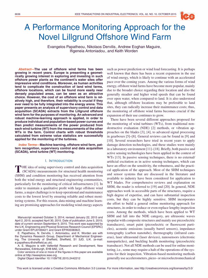
Fig. 1. Location of the 48 turbines in Lillgrund wind farm [40].

II. DESCRIPTION OF THE LILLGRUND WIND FARM

AND THE NOVEL ELEMENT

The Lillgrund wind farm is situated in the sea area betweenDenmark and Sweden and consists of 48 identical WTs of2.3-MW rated power [40]; their distribution is shown in Fig. 1.The wind farm is owned and operated by Vattenfall. Theoriginal labeling of the turbines made use of a combination ofletters and numbers (rows A to D, see again Fig. 1), but for con-venience here, the turbines were simply numbered from 1 to 48.In this paper, only the pure number labeling is going to be used.The separation between the turbines in the row is 3.3×D,where D is the diameter of the turbine, and the rows areseparated by 4.3×D (see Fig. 1). The WTs are Siemens SWT-2.3-93 (see Fig. 2), which are characterized by a rotor diameterof 92.6 m and a hub height of 65 m, giving a rated power of2.3 MW. The maximum rated power is reached when windspeeds take values of 12 m/s (rated wind speed).

It is important to note that the spacing between the tur-bines in the specific wind farm is significantly closer thanmost conventional farms [40], and this unique element is gen-erally expected to affect their performance. This wind farmarchitecture was created deliberately for analyzing the effectsand the interactions of each WT within such closer spacing.The available data used in this study correspond to a fullyear of operation. All the SCADA extracts consist of 10-minaverages, with the maximum, mean, minimum, and standarddeviation of the 10-min intervals being recorded and available.The actual sampling frequency is less than 10 min, but it is notdisclosed here.

III. POWER CURVE MONITORING OF WTs

The number of sources of information regarding reliability ofWT technology lifetimes is very limited due to the highly com-petitive market. Offshore wind farms are arguably going to bethe pioneers in future regarding the renewable energy sources;however, because they operate in remote areas away from landand are expanding into deeper waters, SHM will be an essen-tial part of the success of these structures in the competitivemarket. Automatic mechanisms for anomalous performance


Fig. 2. Siemens SWT-2.3-93 in Lillgrund [40].

detection of the WTs are still in the embryonic stage. Followingthese thoughts, a view of sensitive and robust damage detec-tion methodologies of signal processing is investigated in thispaper.

Once more, one has to recall from before that the rare spacing(worldwide) between the turbines is one of the most challengingand interesting motivations behind the analysis of this work.The analysis is based on neural network and GP regressionand is used to predict the measurement of each WT fromthe measurements of other WTs in the farm. Neural networksare standard machine-learning tools, and they were the firstto be applied, but as will be shown, GPs have certain usefuladvantages. Regression model error is used as an index ofabnormal response. Furthermore, as will be seen later using thisregression error (residual error, which is the difference betweenthe algorithm predictions and the actual SCADA data), a strongvisualization that indicates when faults occur will be presented.

A key novel technique in computing these warning levels(thresholds), which indicate novelty (faults), is the usage ofsophisticated tools in order to obtain these thresholds. As willbe explained later, the warning levels are calculated by usingEVS via evolutionary optimization algorithms such as the self-adaptive differential evolution (DE).

A. ANNs

Artificial neural networks (ANNs) are algorithms or, to bemore specific, mathematical models, which are loosely basedon the way that the human brain and biological neurons work.

They have been extensively used for regression and classifi-cation, and they have been very successful in modeling dataoriginating from various different sources. In the current work,the multilayer perceptron (MLP), i.e., the most common neuralnetwork, is used [41]. For more details on the MLPs, the readeris referred to [41] and [42]. Since neural networks have beensuccessfully used for nonlinear regression, they seem ideal forlearning the power curve of WTs. The wind speed is available,in 10-min averages, from the SCADA extracts for each turbine(there is an anemometer in each tower). In addition, the SCADAdata provide a status for the operation of the turbines, usuallyin the form of an “error code.” For the creation of the healthypower curve (the reference curve), data from the whole yearwere used, but only when they corresponded to time instanceswith a status code equal to “0,” which means “no error” in theturbines. The one-year healthy data were separated into train-ing, validation, and testing sets. The training set is primarilyused for the training of the networks, whereas the validationis used to identify the best structure for the network. Differentnumbers of training cycles are applied, and in the end, thefinally selected network is tested with fresh data with the helpof the testing set. The search for the network structure here wentfrom one up to ten hidden units, and the finally selected numberof training cycles used was 300. All the training was donewith the help of the Netlab [43] package, and the optimizationalgorithm for the network output error minimization was thescaled conjugate gradient method [43], [44]. The measure of thegoodness of the regression fit was provided by the normalizedmean-square error (MSE) shown in

MSE(y) =100

Nσ2y

n∑

i=1

(yi − yi)2 (1)

where the caret denotes an estimated quantity, yi is the actualobservation, N is the total number of observations, and σy isthe standard deviation.

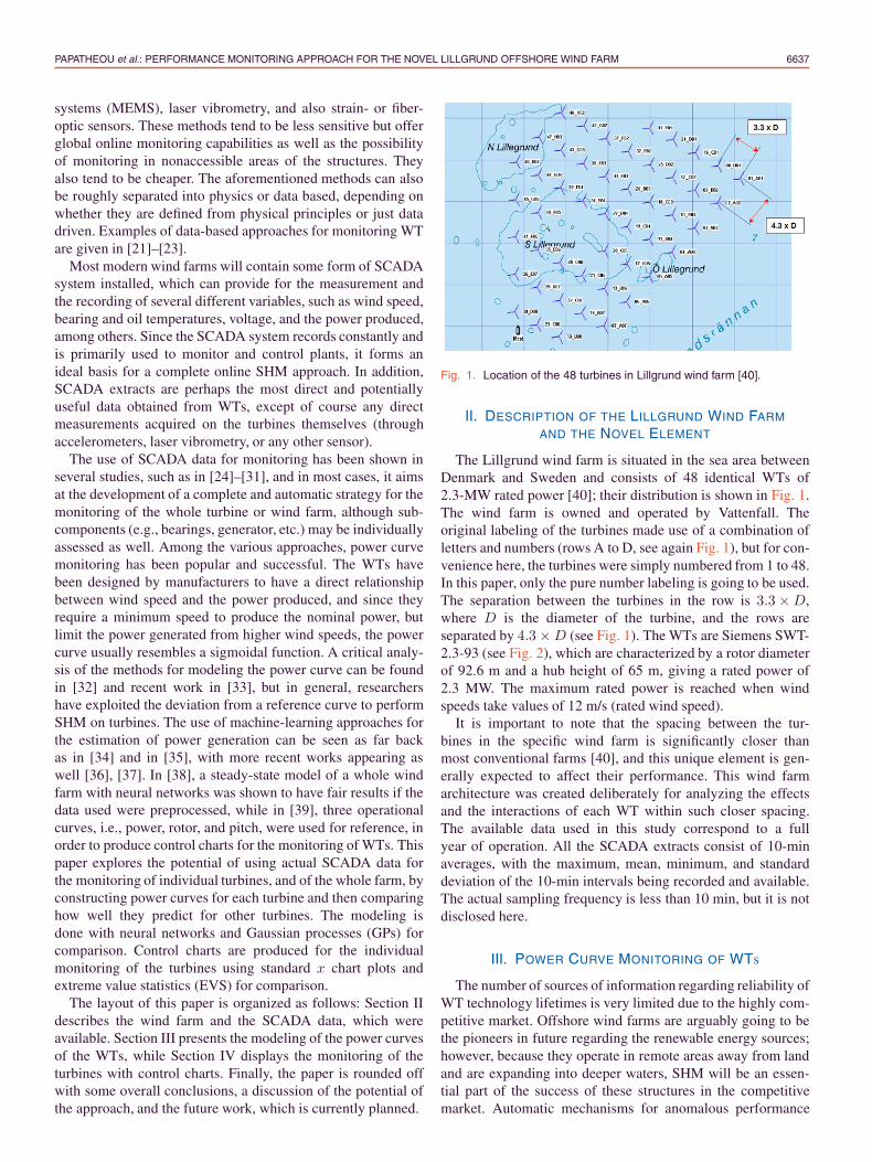
In total, 48 different networks (same as the number of tur-bines) were finally selected to create a power reference curvefor the turbines. After that, each network was provided withwind speed data from the rest of the turbines and was asked topredict the power produced from them. In Fig. 3, the normalizedMSE errors of each trained network, when tested with windspeed data for the turbine for which they were trained, andsubsequently the remaining turbines, is shown. Each axis ofthe confusion matrix shown in Fig. 3 corresponds to 1 up to48 turbines, where on the y-axis is the number of the trainedturbine and on the x-axis the number of the tested turbine. Ingeneral, an MSE error below 5 is considered a good fit andbelow 1 excellent.

From the results, it is clear that almost all the trained net-works are very robust and the maximum MSE error is around5, which mainly occurs in turbines 3 and 4, which are locatedin the outside row of the wind farm. It can also be seen that,on the diagonal of the confusion matrix (which correspondsto the testing set of the trained turbines when tested withdata from themselves), the MSE error is very low, with themaximum appearing in turbine 39 (MSE = 1.4708) and the


Fig. 3. Confusion matrix with MSE errors created from the neuralnetworks: testing set.

Fig. 4. MSE error of the neural network models when presented withdata not corresponding to error code “0.”

minimum in turbine 31 with MSE at 0.5408. When the trainednetworks for an individual turbine were fed data originatingfrom the same network, but which did not correspond to “noerror statuses,” the MSE error was everywhere larger, as shownin Fig. 4; the lowest was 4.7991, which appeared in turbine 12,and it was still larger than the 0.8262 of the healthy data.In turbine 4, for example, the MSE increased from 0.768 to149.033 and the standard deviation of the regression error from0.0593 to 0.3685. Subsequent scanning of the data revealedthat the majority of the instances where the regression errorbecomes high (in turbine 4) happened when the turbine wasnot working, either from emergency stops or manual stops.The emergency stops are associated with faults, but as theseresults derive from actual working data, the types of faultsare limited to what was present during the recording period.Essentially, Fig. 3 shows a map of potential thresholds, whichcan be used for the monitoring (in a novelty detection scheme)of the turbines individually or as a population.

B. GPs

Neural networks have proved to be a very powerful tool,particularly for nonlinear regression, but they also presentseveral challenges during their modeling stage. The structureof the network, including hidden layers and hidden nodes alongwith the training cycles, plays a prominent role in the accuratemodeling of data and the overall results of any such analysis.In addition, different initial conditions for the network weightsmust always be explored, and issues regarding overfitting ofdata are generally present, making the process nontrivial.

Alternatively, in the area of monitoring a WT via a regres-sion analysis and in the exact same philosophy as the onedescribed earlier, another powerful technique can be adopted,which is much simpler and faster. This technique is the GP forregression. The GP is a research area of increasing interest,not only for regression but also for classification purposes.The GP is a stochastic nonparametric Bayesian approach toregression and classification problems. These GPs are compu-tationally very efficient, and the nonlinear learning is relativelyeasy. Regression with these algorithms takes into account allpossible functions that fit to the training data vector and givesa predictive distribution of a single prediction for a giveninput vector. As a result, a mean prediction and confidenceintervals on this prediction can be calculated from this pre-dictive distribution. For more details, the reader is referred to[42] and [45].

The initial and basic steps in order to apply GP regressionis to obtain mean and covariance functions. These functionsare specified separately and consist of a specification of afunctional form and a set of parameters called hyperparam-eters. Here, a zero-mean function and a squared-exponentialcovariance function are applied (see [45]). When the mean andcovariance functions are defined, then the inference methodspecifies the calculation of the exact model and, in simpleterms, describes how to compute hyperparameters by mini-mization of the negative log marginal likelihood. The softwareused for the implementation of GP regression was providedin [45].

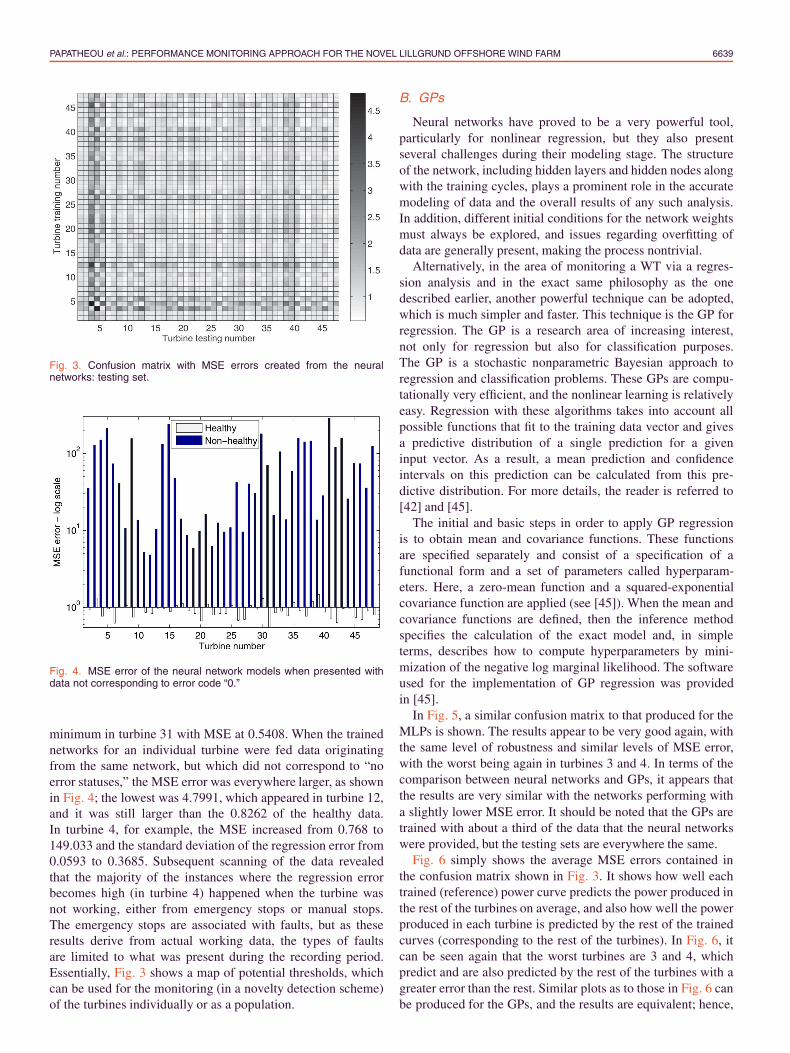
In Fig. 5, a similar confusion matrix to that produced for theMLPs is shown. The results appear to be very good again, withthe same level of robustness and similar levels of MSE error,with the worst being again in turbines 3 and 4. In terms of thecomparison between neural networks and GPs, it appears thatthe results are very similar with the networks performing witha slightly lower MSE error. It should be noted that the GPs aretrained with about a third of the data that the neural networkswere provided, but the testing sets are everywhere the same.

Fig. 6 simply shows the average MSE errors contained inthe confusion matrix shown in Fig. 3. It shows how well eachtrained (reference) power curve predicts the power produced inthe rest of the turbines on average, and also how well the powerproduced in each turbine is predicted by the rest of the trainedcurves (corresponding to the rest of the turbines). In Fig. 6, itcan be seen again that the worst turbines are 3 and 4, whichpredict and are also predicted by the rest of the turbines with agreater error than the rest. Similar plots as to those in Fig. 6 canbe produced for the GPs, and the results are equivalent; hence,


Fig. 5. Confusion matrix with MSE errors created from the GPs:testing set.

Fig. 6. Average MSE error showing (a) how well the power producedin each turbine is predicted by the networks trained in the rest of theturbines and (b) how well each trained network produces the powerproduced in the other turbines.

they are not included here. The very low MSE errors show thatthe power curves have the potential of being used as a featurefor the monitoring of the whole farm, as they were shownto be generally robust to the individual differences that theturbines inevitably present (location, different sensors, differentgenerators, etc).

IV. VISUALIZING THE DATA USING GP ANALYSIS

THROUGH ROBUST EVS THRESHOLDS

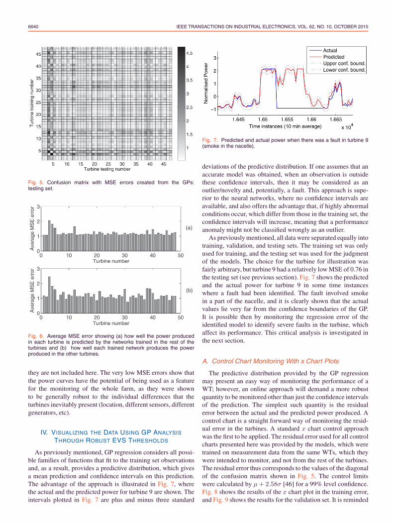
As previously mentioned, GP regression considers all possi-ble families of functions that fit to the training set observationsand, as a result, provides a predictive distribution, which givesa mean prediction and confidence intervals on this prediction.The advantage of the approach is illustrated in Fig. 7, wherethe actual and the predicted power for turbine 9 are shown. Theintervals plotted in Fig. 7 are plus and minus three standard

Fig. 7. Predicted and actual power when there was a fault in turbine 9(smoke in the nacelle).

deviations of the predictive distribution. If one assumes that anaccurate model was obtained, when an observation is outsidethese confidence intervals, then it may be considered as anoutlier/novelty and, potentially, a fault. This approach is supe-rior to the neural networks, where no confidence intervals areavailable, and also offers the advantage that, if highly abnormalconditions occur, which differ from those in the training set, theconfidence intervals will increase, meaning that a performanceanomaly might not be classified wrongly as an outlier.

As previously mentioned, all data were separated equally intotraining, validation, and testing sets. The training set was onlyused for training, and the testing set was used for the judgmentof the models. The choice for the turbine for illustration wasfairly arbitrary, but turbine 9 had a relatively low MSE of 0.76 inthe testing set (see previous section). Fig. 7 shows the predictedand the actual power for turbine 9 in some time instanceswhere a fault had been identified. The fault involved smokein a part of the nacelle, and it is clearly shown that the actualvalues lie very far from the confidence boundaries of the GP.It is possible then by monitoring the regression error of theidentified model to identify severe faults in the turbine, whichaffect its performance. This critical analysis is investigated inthe next section.

A. Control Chart Monitoring With x Chart Plots

The predictive distribution provided by the GP regressionmay present an easy way of monitoring the performance of aWT; however, an online approach will demand a more robustquantity to be monitored other than just the confidence intervalsof the prediction. The simplest such quantity is the residualerror between the actual and the predicted power produced. Acontrol chart is a straight forward way of monitoring the resid-ual error in the turbines. A standard x chart control approachwas the first to be applied. The residual error used for all controlcharts presented here was provided by the models, which weretrained on measurement data from the same WTs, which theywere intended to monitor, and not from the rest of the turbines.The residual error thus corresponds to the values of the diagonalof the confusion matrix shown in Fig. 5. The control limitswere calculated by μ+ 2.58σ [46] for a 99% level confidence.Fig. 8 shows the results of the x chart plot in the training error,and Fig. 9 shows the results for the validation set. It is reminded


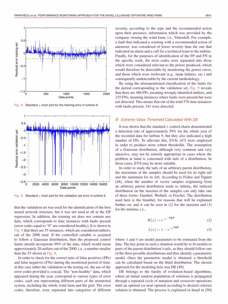
Fig. 8. Standard x chart plot for the training error in turbine 9.

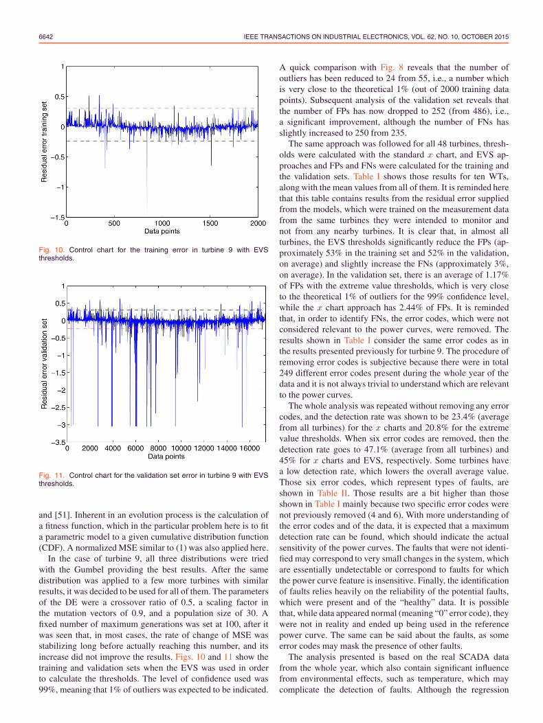
Fig. 9. Standard x chart plot for the validation set error in turbine 9.

that the validation set was used for the identification of the bestneural network structure, but it was not used at all in the GPregression. In addition, the training set does not contain anydata, which corresponds to time instances with faults present(error codes equal to “0” are considered healthy). It is shown inFig. 8 that there are 55 instances, which are considered outliers,out of the 2000 total. If the controlled variable is assumedto follow a Gaussian distribution, then the proposed controllimits should incorporate 99% of the data, which would meanapproximately 20 outliers out of the 2000, i.e., a number smallerthan the 55 shown in Fig. 8.

In order to check for the correct ratio of false positives (FPs)and false negatives (FNs) during the monitored period of time,in this case either the validation or the testing set, the use of theerror codes provided is crucial. The “non-healthy” data, whichappeared during the year, correspond to various types of errorcodes, each one representing different parts of the monitoredsystem, including the whole wind farm and the grid. The errorcodes, therefore, were separated into categories of different

severity, according to the type and the recommended actionupon their presence, information which was provided by thecompany owning the wind farm, i.e., Vattenfall. For example,a fault that indicated a warning with a recommended action ofautoreset, was considered of lower severity than the one thatindicated an alarm and a call for a technical team to the turbine.Finally, for the purposes of identification of the FP and FN inthe specific work, the error codes were separated into thosewhich were considered relevant to the power produced, whichwould therefore be detectable by monitoring the power curve,and those which were irrelevant (e.g., lamp failures, etc.) andconsequently undetectable by the current methodology.

By using the aforementioned classification of the faults forthe period corresponding to the validation set, Fig. 9 revealsthat there are 486 FPs, meaning wrongly identified outliers, and235 FNs, meaning instances where faults were present but werenot detected. This means that out of the total 576 time instanceswith faults present, 341 were detected.

B. Extreme Value Threshold Calculated With DE

It was shown that the standard x control charts demonstrateda detection rate of approximately 59% for the whole year ofthe recorded data for turbine 9, but they also indicated a highnumber of FPs. To alleviate this, EVSs [47] were employedin order to produce more robust thresholds. The assumptionof a Gaussian distribution, although very common and veryattractive, may not be entirely appropriate in cases where theproblem at hand is concerned with tails of a distribution. Inthose cases, EVS may be more suitable.

In order to study the tails of an arbitrary parent distribution,the maximum of the samples should be used for its right tailand the minimum for its left. According to Fisher and Tippett[48], when the number of vector samples originating froman arbitrary parent distribution tends to infinity, the induceddistribution on the maxima of the samples can only take oneof three forms: Gumbel, Weibull, or Frechet. The distributionused here is the Gumbel, for reasons that will be explainedfurther on, and it can be seen in (2) for the maxima and (3)for the minima, i.e.,

H(x) = e−e− x−λ

δ (2)

L(x) = 1− e−ex−λ

δ (3)

where λ and δ are model parameters to be estimated from thedata. The key point in such a situation would be to fit models toparts of the parent distribution’s tails, as they should follow oneof the three possible distributions and thus identify a parametricmodel. Once the parametric model is obtained, a thresholdcan be calculated based on the fitted distribution. The chosenapproach for the modeling here was DE [49].

DE belongs to the family of evolution-based algorithms,where an initial random population of solutions is propagatedthrough a repeated cycle of mutation and crossover operationsuntil an optimal (or near optimal according to desired criteria)solution is obtained. The process is explained in detail in [50]


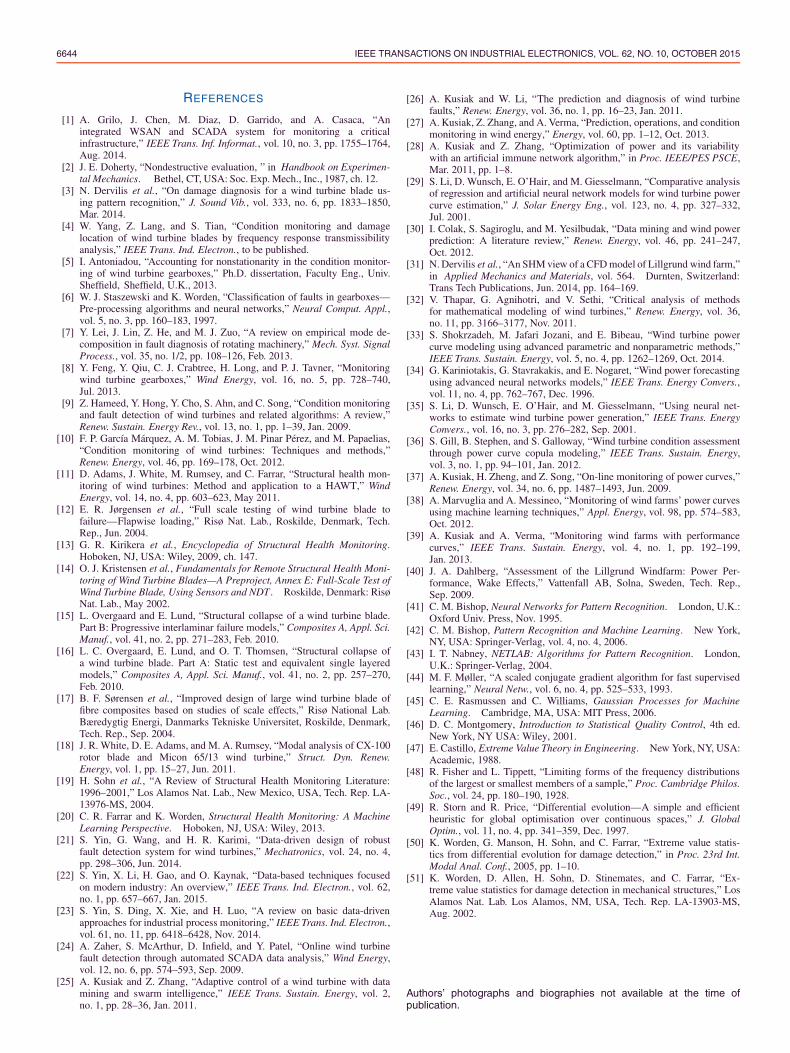
Fig. 10. Control chart for the training error in turbine 9 with EVSthresholds.

Fig. 11. Control chart for the validation set error in turbine 9 with EVSthresholds.

and [51]. Inherent in an evolution process is the calculation ofa fitness function, which in the particular problem here is to fita parametric model to a given cumulative distribution function(CDF). A normalized MSE similar to (1) was also applied here.

In the case of turbine 9, all three distributions were triedwith the Gumbel providing the best results. After the samedistribution was applied to a few more turbines with similarresults, it was decided to be used for all of them. The parametersof the DE were a crossover ratio of 0.5, a scaling factor inthe mutation vectors of 0.9, and a population size of 30. Afixed number of maximum generations was set at 100, after itwas seen that, in most cases, the rate of change of MSE wasstabilizing long before actually reaching this number, and itsincrease did not improve the results. Figs. 10 and 11 show thetraining and validation sets when the EVS was used in orderto calculate the thresholds. The level of confidence used was99%, meaning that 1% of outliers was expected to be indicated.

A quick comparison with Fig. 8 reveals that the number ofoutliers has been reduced to 24 from 55, i.e., a number whichis very close to the theoretical 1% (out of 2000 training datapoints). Subsequent analysis of the validation set reveals thatthe number of FPs has now dropped to 252 (from 486), i.e.,a significant improvement, although the number of FNs hasslightly increased to 250 from 235.

The same approach was followed for all 48 turbines, thresh-olds were calculated with the standard x chart, and EVS ap-proaches and FPs and FNs were calculated for the training andthe validation sets. Table I shows those results for ten WTs,along with the mean values from all of them. It is reminded herethat this table contains results from the residual error suppliedfrom the models, which were trained on the measurement datafrom the same turbines they were intended to monitor andnot from any nearby turbines. It is clear that, in almost allturbines, the EVS thresholds significantly reduce the FPs (ap-proximately 53% in the training set and 52% in the validation,on average) and slightly increase the FNs (approximately 3%,on average). In the validation set, there is an average of 1.17%of FPs with the extreme value thresholds, which is very closeto the theoretical 1% of outliers for the 99% confidence level,while the x chart approach has 2.44% of FPs. It is remindedthat, in order to identify FNs, the error codes, which were notconsidered relevant to the power curves, were removed. Theresults shown in Table I consider the same error codes as inthe results presented previously for turbine 9. The procedure ofremoving error codes is subjective because there were in total249 different error codes present during the whole year of thedata and it is not always trivial to understand which are relevantto the power curves.

The whole analysis was repeated without removing any errorcodes, and the detection rate was shown to be 23.4% (averagefrom all turbines) for the x charts and 20.8% for the extremevalue thresholds. When six error codes are removed, then thedetection rate goes to 47.1% (average from all turbines) and45% for x charts and EVS, respectively. Some turbines havea low detection rate, which lowers the overall average value.Those six error codes, which represent types of faults, areshown in Table II. Those results are a bit higher than thoseshown in Table I mainly because two specific error codes werenot previously removed (4 and 6). With more understanding ofthe error codes and of the data, it is expected that a maximumdetection rate can be found, which should indicate the actualsensitivity of the power curves. The faults that were not identi-fied may correspond to very small changes in the system, whichare essentially undetectable or correspond to faults for whichthe power curve feature is insensitive. Finally, the identificationof faults relies heavily on the reliability of the potential faults,which were present and of the “healthy” data. It is possiblethat, while data appeared normal (meaning “0” error code), theywere not in reality and ended up being used in the referencepower curve. The same can be said about the faults, as someerror codes may mask the presence of other faults.

The analysis presented is based on the real SCADA datafrom the whole year, which also contain significant influencefrom environmental effects, such as temperature, which maycomplicate the detection of faults. Although the regression


TABLE IFPS AND FNS FOR TEN WIND TURBINES AND THE MEAN VALUES FROM ALL 48. DR STANDS FOR DETECTION RATE. THE MODELS

USED HERE WERE TRAINED ON DATA FROM THE SAME WTS AS THOSE THEY WERE INTENDED TO MONITOR

TABLE IIEXAMPLES OF ERROR CODES THAT WERE REMOVED FROM

THE ANALYSIS (THE NUMBERS DO NOT CORRESPONDTO THE ACTUAL CODES USED IN THE SCADA)

error was shown to be small for the whole year, it is possiblethat modeling the power curves on a smaller time scale, e.g.,monthly or weekly, will probably increase the detection offaults, but this may require the frequent update of the referencepower curve. In addition, the SCADA data currently usedare 10-min averages, which may also be a reason for lowerdetection of faults; it is expected that 1-min data will improvethe results. The approach does not require a complex physics-based model of the WTs and does not preprocess the data orfilter out potential outliers; it is generally straightforward toapply since it only requires wind measurements and powerproduced for the development of a reference curve.

The results shown in this paper were presented for x chartplots under an assumption of Gaussian statistics and using EVSdistributions. It is shown that the EVSs provide the appropriatethresholds for a given confidence level. One could argue thatbetter thresholds could be obtained by using an x chart. Thisis certainly true; however, it requires grouping the data. Forexample, assuming a group size of 12 here for an x chart wouldmean that diagnostic results would only be checked every 2 hinstead of 10 min.

V. CONCLUSION

This paper has presented an exploration of the suitability ofSCADA extracts from the Lillgrund wind farm for the purposesof monitoring the farm via sophisticated machine-learning ar-chitectures. ANNs and GPs were used to build a referencepower curve (wind speed versus power produced) for each ofthe 48 turbines existing in the farm and as well as EVS viaan optimization algorithm in order to define alarm thresholds.Then, each reference model was used to predict the powerproduced in the rest of the turbines available, thus creating aconfusion matrix of the MSE errors for all combinations. Theresults showed that nearly all models were very robust withthe highest MSE error to be 4.8291, and this was happeningwhen the model trained in turbine 4 was predicting power fromturbine 3. Both turbines 3 and 4 are located in the outside rowof the wind farm. It was shown that, when wind speed data,which did not come from time instances where the error statuswas “0” (meaning healthy data), were used as an input to thetrained neural networks, the MSE error was significantly largerfor neural networks and GPs. Comparison between neuralnetworks and GPs showed that there is no significant differencein their performance, but the inherent ability of the GPs toproduce confidence intervals is advantageous. The residuals ofthe models, which used data from the same turbines, which theywere intended to monitor, were next used in a novelty detectionscheme. It was shown that it is possible to monitor significantevents that will affect the performance of the turbines by simplecontrol charts, although certain faults remained undetected.An approach for the calculation of robust thresholds in theresiduals made use of EVS and showed a significant reductionin the number of FPs. Future work will also focus on extrafeatures other than the power curve for the improvement of theapproach. In addition, the full analysis of the error statuses thatwere presented during the recorded time can lead to a moreintelligent identification of faults, including their classification.


REFERENCES

[1] A. Grilo, J. Chen, M. Diaz, D. Garrido, and A. Casaca, “Anintegrated WSAN and SCADA system for monitoring a criticalinfrastructure,” IEEE Trans. Inf. Informat., vol. 10, no. 3, pp. 1755–1764,Aug. 2014.

[2] J. E. Doherty, “Nondestructive evaluation, ” in Handbook on Experimen-tal Mechanics. Bethel, CT, USA: Soc. Exp. Mech., Inc., 1987, ch. 12.

[3] N. Dervilis et al., “On damage diagnosis for a wind turbine blade us-ing pattern recognition,” J. Sound Vib., vol. 333, no. 6, pp. 1833–1850,Mar. 2014.

[4] W. Yang, Z. Lang, and S. Tian, “Condition monitoring and damagelocation of wind turbine blades by frequency response transmissibilityanalysis,” IEEE Trans. Ind. Electron., to be published.

[5] I. Antoniadou, “Accounting for nonstationarity in the condition monitor-ing of wind turbine gearboxes,” Ph.D. dissertation, Faculty Eng., Univ.Sheffield, Sheffield, U.K., 2013.

[6] W. J. Staszewski and K. Worden, “Classification of faults in gearboxes—Pre-processing algorithms and neural networks,” Neural Comput. Appl.,vol. 5, no. 3, pp. 160–183, 1997.

[7] Y. Lei, J. Lin, Z. He, and M. J. Zuo, “A review on empirical mode de-composition in fault diagnosis of rotating machinery,” Mech. Syst. SignalProcess., vol. 35, no. 1/2, pp. 108–126, Feb. 2013.

[8] Y. Feng, Y. Qiu, C. J. Crabtree, H. Long, and P. J. Tavner, “Monitoringwind turbine gearboxes,” Wind Energy, vol. 16, no. 5, pp. 728–740,Jul. 2013.

[9] Z. Hameed, Y. Hong, Y. Cho, S. Ahn, and C. Song, “Condition monitoringand fault detection of wind turbines and related algorithms: A review,”Renew. Sustain. Energy Rev., vol. 13, no. 1, pp. 1–39, Jan. 2009.

[10] F. P. García Márquez, A. M. Tobias, J. M. Pinar Pérez, and M. Papaelias,“Condition monitoring of wind turbines: Techniques and methods,”Renew. Energy, vol. 46, pp. 169–178, Oct. 2012.

[11] D. Adams, J. White, M. Rumsey, and C. Farrar, “Structural health mon-itoring of wind turbines: Method and application to a HAWT,” WindEnergy, vol. 14, no. 4, pp. 603–623, May 2011.

[12] E. R. Jørgensen et al., “Full scale testing of wind turbine blade tofailure—Flapwise loading,” Risø Nat. Lab., Roskilde, Denmark, Tech.Rep., Jun. 2004.

[13] G. R. Kirikera et al., Encyclopedia of Structural Health Monitoring.Hoboken, NJ, USA: Wiley, 2009, ch. 147.

[14] O. J. Kristensen et al., Fundamentals for Remote Structural Health Moni-toring of Wind Turbine Blades—A Preproject, Annex E: Full-Scale Test ofWind Turbine Blade, Using Sensors and NDT. Roskilde, Denmark: RisøNat. Lab., May 2002.

[15] L. Overgaard and E. Lund, “Structural collapse of a wind turbine blade.Part B: Progressive interlaminar failure models,” Composites A, Appl. Sci.Manuf., vol. 41, no. 2, pp. 271–283, Feb. 2010.

[16] L. C. Overgaard, E. Lund, and O. T. Thomsen, “Structural collapse ofa wind turbine blade. Part A: Static test and equivalent single layeredmodels,” Composites A, Appl. Sci. Manuf., vol. 41, no. 2, pp. 257–270,Feb. 2010.

[17] B. F. Sørensen et al., “Improved design of large wind turbine blade offibre composites based on studies of scale effects,” Risø National Lab.Bæredygtig Energi, Danmarks Tekniske Universitet, Roskilde, Denmark,Tech. Rep., Sep. 2004.

[18] J. R. White, D. E. Adams, and M. A. Rumsey, “Modal analysis of CX-100rotor blade and Micon 65/13 wind turbine,” Struct. Dyn. Renew.Energy, vol. 1, pp. 15–27, Jun. 2011.

[19] H. Sohn et al., “A Review of Structural Health Monitoring Literature:1996–2001,” Los Alamos Nat. Lab., New Mexico, USA, Tech. Rep. LA-13976-MS, 2004.

[20] C. R. Farrar and K. Worden, Structural Health Monitoring: A MachineLearning Perspective. Hoboken, NJ, USA: Wiley, 2013.

[21] S. Yin, G. Wang, and H. R. Karimi, “Data-driven design of robustfault detection system for wind turbines,” Mechatronics, vol. 24, no. 4,pp. 298–306, Jun. 2014.

[22] S. Yin, X. Li, H. Gao, and O. Kaynak, “Data-based techniques focusedon modern industry: An overview,” IEEE Trans. Ind. Electron., vol. 62,no. 1, pp. 657–667, Jan. 2015.

[23] S. Yin, S. Ding, X. Xie, and H. Luo, “A review on basic data-drivenapproaches for industrial process monitoring,” IEEE Trans. Ind. Electron.,vol. 61, no. 11, pp. 6418–6428, Nov. 2014.

[24] A. Zaher, S. McArthur, D. Infield, and Y. Patel, “Online wind turbinefault detection through automated SCADA data analysis,” Wind Energy,vol. 12, no. 6, pp. 574–593, Sep. 2009.

[25] A. Kusiak and Z. Zhang, “Adaptive control of a wind turbine with datamining and swarm intelligence,” IEEE Trans. Sustain. Energy, vol. 2,no. 1, pp. 28–36, Jan. 2011.

[26] A. Kusiak and W. Li, “The prediction and diagnosis of wind turbinefaults,” Renew. Energy, vol. 36, no. 1, pp. 16–23, Jan. 2011.

[27] A. Kusiak, Z. Zhang, and A. Verma, “Prediction, operations, and conditionmonitoring in wind energy,” Energy, vol. 60, pp. 1–12, Oct. 2013.

[28] A. Kusiak and Z. Zhang, “Optimization of power and its variabilitywith an artificial immune network algorithm,” in Proc. IEEE/PES PSCE,Mar. 2011, pp. 1–8.

[29] S. Li, D. Wunsch, E. O’Hair, and M. Giesselmann, “Comparative analysisof regression and artificial neural network models for wind turbine powercurve estimation,” J. Solar Energy Eng., vol. 123, no. 4, pp. 327–332,Jul. 2001.

[30] I. Colak, S. Sagiroglu, and M. Yesilbudak, “Data mining and wind powerprediction: A literature review,” Renew. Energy, vol. 46, pp. 241–247,Oct. 2012.

[31] N. Dervilis et al., “An SHM view of a CFD model of Lillgrund wind farm,”in Applied Mechanics and Materials, vol. 564. Durnten, Switzerland:Trans Tech Publications, Jun. 2014, pp. 164–169.

[32] V. Thapar, G. Agnihotri, and V. Sethi, “Critical analysis of methodsfor mathematical modeling of wind turbines,” Renew. Energy, vol. 36,no. 11, pp. 3166–3177, Nov. 2011.

[33] S. Shokrzadeh, M. Jafari Jozani, and E. Bibeau, “Wind turbine powercurve modeling using advanced parametric and nonparametric methods,”IEEE Trans. Sustain. Energy, vol. 5, no. 4, pp. 1262–1269, Oct. 2014.

[34] G. Kariniotakis, G. Stavrakakis, and E. Nogaret, “Wind power forecastingusing advanced neural networks models,” IEEE Trans. Energy Convers.,vol. 11, no. 4, pp. 762–767, Dec. 1996.

[35] S. Li, D. Wunsch, E. O’Hair, and M. Giesselmann, “Using neural net-works to estimate wind turbine power generation,” IEEE Trans. EnergyConvers., vol. 16, no. 3, pp. 276–282, Sep. 2001.

[36] S. Gill, B. Stephen, and S. Galloway, “Wind turbine condition assessmentthrough power curve copula modeling,” IEEE Trans. Sustain. Energy,vol. 3, no. 1, pp. 94–101, Jan. 2012.

[37] A. Kusiak, H. Zheng, and Z. Song, “On-line monitoring of power curves,”Renew. Energy, vol. 34, no. 6, pp. 1487–1493, Jun. 2009.

[38] A. Marvuglia and A. Messineo, “Monitoring of wind farms’ power curvesusing machine learning techniques,” Appl. Energy, vol. 98, pp. 574–583,Oct. 2012.

[39] A. Kusiak and A. Verma, “Monitoring wind farms with performancecurves,” IEEE Trans. Sustain. Energy, vol. 4, no. 1, pp. 192–199,Jan. 2013.

[40] J. A. Dahlberg, “Assessment of the Lillgrund Windfarm: Power Per-formance, Wake Effects,” Vattenfall AB, Solna, Sweden, Tech. Rep.,Sep. 2009.

[41] C. M. Bishop, Neural Networks for Pattern Recognition. London, U.K.:Oxford Univ. Press, Nov. 1995.

[42] C. M. Bishop, Pattern Recognition and Machine Learning. New York,NY, USA: Springer-Verlag, vol. 4, no. 4, 2006.

[43] I. T. Nabney, NETLAB: Algorithms for Pattern Recognition. London,U.K.: Springer-Verlag, 2004.

[44] M. F. Møller, “A scaled conjugate gradient algorithm for fast supervisedlearning,” Neural Netw., vol. 6, no. 4, pp. 525–533, 1993.

[45] C. E. Rasmussen and C. Williams, Gaussian Processes for MachineLearning. Cambridge, MA, USA: MIT Press, 2006.

[46] D. C. Montgomery, Introduction to Statistical Quality Control, 4th ed.New York, NY USA: Wiley, 2001.

[47] E. Castillo, Extreme Value Theory in Engineering. New York, NY, USA:Academic, 1988.

[48] R. Fisher and L. Tippett, “Limiting forms of the frequency distributionsof the largest or smallest members of a sample,” Proc. Cambridge Philos.Soc., vol. 24, pp. 180–190, 1928.

[49] R. Storn and R. Price, “Differential evolution—A simple and efficientheuristic for global optimisation over continuous spaces,” J. GlobalOptim., vol. 11, no. 4, pp. 341–359, Dec. 1997.

[50] K. Worden, G. Manson, H. Sohn, and C. Farrar, “Extreme value statis-tics from differential evolution for damage detection,” in Proc. 23rd Int.Modal Anal. Conf., 2005, pp. 1–10.

[51] K. Worden, D. Allen, H. Sohn, D. Stinemates, and C. Farrar, “Ex-treme value statistics for damage detection in mechanical structures,” LosAlamos Nat. Lab. Los Alamos, NM, USA, Tech. Rep. LA-13903-MS,Aug. 2002.

Authors’ photographs and biographies not available at the time ofpublication.

Documents

A Performance Monitoring Approach for the Novel Lillgrund