A Performance Evaluation Method for Climate Coupled Models

Available online at www.sciencedirect.com

1877–0509 © 2011 Published by Elsevier Ltd. Selection and/or peer-review under responsibility of Prof. Mitsuhisa Sato and Prof. Satoshi Matsuokadoi:10.1016/j.procs.2011.04.165

Procedia Computer Science 4 (2011) 1526–1534

International Conference on Computational Science, ICCS 2011

A Performance Evaluation Method for Climate Coupled Models

Italo Epicocoa, *, Silvia Mocaverob, Giovanni Aloisioa,b aUniversity of Salento, via per Monteroni, Lecce 73100, Italy

bEuro-Mediterranean Centre for Climate Change, via Augusto Imperatore, Lecce 73100, Italy

Abstract

In the High Performance Computing context, the performance evaluation of a parallel algorithm is carried out mainly by considering the elapsed time for running the parallel application with both different number of cores and different problem sizes (for scaled speedup). Typically, parallel applications embed mechanisms to efficiently use the allocated resources, guaranteeing for example a good load balancing and reducing the parallel overhead. Unfortunately, this assumption is not true for coupled models. These models were born from the coupling of stand-alone climate models. The component models are developed independently from each other and they follow different development roadmaps. Moreover, they are characterized by different levels of parallelization as well as different requirements in terms of workload and they have their own scalability curve. Considering a coupled model as a single parallel application, we can note the lacking of a policy useful to balance the computational load on the available resources. This work tries to address the issues related to the performance evaluation of a coupled model as well as answering the following questions: once a given number of processors has been allocated for the whole coupled model, how does the run have to be configured in order to balance the workload? How many processors must be assigned to each of the component models? The methodology here described has been applied to evaluate the scalability of the CMCC-MED coupled model designed by the ANS Division of the CMCC. The evaluation has been carried out on two different computational architectures: a scalar cluster, based on IBM Power6 processors, and a vector cluster, based on NEC-SX9 processors. Keywords: HPC; Performance model; Porting; Coupled models

1. Introduction

Different technical solutions are used in the Earth System Modeling (ESM) community to couple climate model codes. Two main approaches, besides hard-coding, can be cited: the use of an external entity, for the transformation of the coupling fields, and linking its communication library to existing applications sometimes referred to as "coupler" approach in the community; the use of coupling library or functions, to build an integrated coupled application based on basilar science units, sometimes referred to as "framework" approach in the community. The different implementations of coupled models in the community lie in the continuum between these two approaches. In the former approach, the component models preserve the original codes almost unchanged and interface each

* Corresponding author. Tel.:+39 0832 297235; fax: +39 0832 297235. E-mail address: [email protected] (Italo Epicoco).

Italo Epicoco et al. / Procedia Computer Science 4 (2011) 1526–1534 1527

other by a communication library. The component models are coupled through an external entity to transform the coupling fields (i.e. the OASIS coupler [1]). This approach results also in a parallel program launched through a MPMD (Multiple Program Multiple Data) [2] approach.

The "framework", or ESMF [3][4], approach foresees a revision of the already developed software modules in order to adapt code data structure to the calling interface of the framework, to split the original code into elemental units, to write or use coupling units and to use the library to build a hierarchical merged code. This approach often results in a single parallel program launched with a SPMD (Single Program Multiple Data) [2] approach. In this case, the MPI2 approach is typically used and the master process spawns the processes for the component models.

A parallel algorithm is mainly evaluated by considering as metrics: the parallel efficiency; the parallel speed-up; and, if we take into account also the problem size, the scaled speed-up. The coupled models differ from the typical scientific parallel application mainly because each of the component models is designed independently from the others; they are characterized by different levels of parallelization, different requirements in terms of workload and they have their own scalability curve. During the design of a coupled model, the effort is mainly focused on the development of the interfaces among the component models and they often lack automatic or dynamic load balancing policies. This implies that the user or modeler has to statically configure the coupled model parameters for balancing the workload among the allocated computational resources. If the total number of processors changes, then the parameters must be re-tuned accordingly.

This work tries to address the issues related to the performance evaluation of a coupled model and to provide an answer to the following question: once the total number of cores allocated for the whole coupled model has been established, how do we have to distribute them for each of the component models?

The paper is organized in three parts: we firstly describe the methodology we have followed to measure the performances of a coupled model; thereafter, we report the results of our analysis performed on a real coupled model used as a case study; we conclude with overall considerations and future direction of the research.

2. Methodology

During the analysis of the scalability of a coupled model, the main issue is to find the best configuration among the component models, in order to obtain a balanced run. The best balancing among different component models could be easily defined if an analytic performance model is provided for each of them. Unfortunately, this cannot be guaranteed every time. In these cases, an experimental analysis is necessary to build the scalability curve of each component. It is worth noting here that the proposed methodology can be applied when an analytic performance model of the components cannot be obtained because they are provided as black boxes or because the definition of an analytic performance model is out of the scope of the research. Four steps compose the methodology we propose: 1. Experimental analysis of each component model, including the coupler, within the coupled model in order to

build the corresponding scalability curves 2. Definition of an analytic performance model, at coarse grain level, of the whole coupled model. The performance

model must take into account the relationship between each component model and the coupler 3. Use of the experimental data given during stage 1, and evaluation of the model defined in stage 2; the best

configurations must be extracted for different numbers of available cores 4. Experimental evaluation of the behavior of the coupled model by considering only the best configurations for a

given number of allocated cores.

3. The CMCC-MED case study

The methodology has been applied to the CMCC-MED [5][6] model developed under the framework of the EU CIRCE Project (Climate Change and Impact Research: the Mediterranean Environment). It provides the possibility to accurately assess the role and feedbacks of the Mediterranean Sea in the global climate system. From a computational point of view, it represents a typical coupled model with a MPMD approach.

This section describes the coupled model with its components, the design of the experiment and the computing environment. Thereafter, a detailed description of the results is presented for each of the four stages of the methodology.

1528 Italo Epicoco et al. / Procedia Computer Science 4 (2011) 1526–1534

3.1. Model description

The CMCC-MED model is a global coupled ocean-atmosphere general circulation model (AOGCM) coupled with a high-resolution model of the Mediterranean Sea. The atmospheric model component (ECHAM5) [7] has a horizontal resolution T159 of about 80 Km with 31 vertical levels, the global ocean model (OPA8.2) [8] has a horizontal resolution of about 2° with an equatorial refinement (0.5°) and 31 vertical levels, the Mediterranean Sea model (NEMO in the MFS implementation [9][10]) has a horizontal resolution of 1/16° (∼7 Km) and 72 vertical levels. The communication between the atmospheric model and the ocean models is performed through the CMCC parallel version of OASIS3 coupler [11], and the exchange of SST, surface momentum, heat, and water fluxes occurs every 2h40m. The total number of fields exchanged through OASIS3 is 35. The global ocean-Mediterranean connection occurs through the exchange of dynamical and tracer fields via simple input/output operations. In particular, horizontal velocities, tracers and sea level are transferred from the global ocean to the Mediterranean model through the open boundaries in the Atlantic box. Similarly, vertical profiles of temperature, salinity and horizontal velocities at the Gibraltar Strait are transferred from the regional Mediterranean model to the global ocean. The ocean-to-ocean exchange occurs with a daily frequency, with the exchanged variables being averaged over the daily time-window.

3.2. Model configuration

In table 1 the compilation keys for each component model are reported. Each component model is used with the spatial and temporal resolutions shown in table 2, while the coupler OASIS3 has been configured as in table 3.

Table 1. Compilation keys for component models.

Model name Compilation keys

NEMO - Mediterranean Sea key_dynspg_flt key_ldfslp key_zdfric key_dtasal key_dtatem key_vectopt_loop key_vectopt_memory key_oasis3 key_coupled key_flx_circe key_obc key_qb5 key_mfs key_cpl_discharge_echam5 key_cpl_ocevel key_mpp_mpi key_cpl_rootexchg key_useexchg

ECHAM5 - Atmospheric __cpl_opa_lim __prism __CLIM_Box __grids_writing __cpl_maskvalue __cpl_wind_stress

OPA8.2 - Ocean Global key_coupled key_coupled_prism key_coupled_echam5 key_coupled_echam5_intB key_orca_r2 key_ice_lln key_lim_fdd key_freesurf_cstvol key_zdftke key_flxqsr key_trahdfiso key_trahdfcoef2d key_dynhdfcoef3d key_trahdfeiv key_convevd key_temdta key_saldta key_coupled_surf_current key_saldta_monthly key_diaznl key_diahth key_monotasking

Table 2. Spatial and temporal resolution of the component models.

OPA8.2 ECHAM5 NEMO

Time step (sec) 4800 240 600

Grid points 182x149 480x240 871x253

Vertical levels 31 31 72

Table 3. OASIS3 configuration.

OASIS3 configuration

Coupling period (sec) 9600

Total number of fields to be transformed 35

Number of fields exported to Number of fields imported from LAG (sec)

OPA8.2 17 6 4800

ECHAM5 9 26 240

NEMO 9 3 600


3.3. Computing environment

All of the experiments have been carried out on two different architectures available at the CMCC Supercomputing Centre: a scalar cluster based on IBM Power6 processors and a vector cluster based on NEC-SX9 processors.

The IBM cluster, named Calypso, has 30 IBM p575 nodes, each one equipped with 16 Power6 dual-core CPUs at 4.7GHz (8MB L2/DCM, 32MB L3/DCM). With Simultaneous Multi Threading (SMT) support enabled, each node hosts 64 virtual cores. The whole cluster provides a computational power of 18 TFLOPS. Each node has 128GB of shared memory (4GB per core), two local SAS disks of 146,8GB at 10k RPM and two Infiniband network cards, each one with four 4X IB galaxy-2 and four Gigabit network adapters. Some nodes are used as GPFS and TSM servers and have also two fibre channel adapters at 4Gb/s FC and two fibre channel adapters at 8Gb/s for the interconnection with the storage system. Calypso has 2 storage racks, each one equipped with 280 disks of 750GB, providing a total capacity of 210TB of raw storage. These disks are working with GPFS. Calypso interconnects also a tape library with 1280 cartridges LTO4 at 800GB (1PB total capacity) and Tivoli TSM to handle Hierarchical Storage Management. The default compilers are IBM XL C/C++, and IBM XL FORTRAN. The default resource scheduler manager is LSF.

The NEC cluster, named Ulysses, has 7 nodes based on SX9 processors. Each node has 16 CPUs at 3.2GHz, 512GB of shared memory, a local SAS D3-10 disk of 3.4TB and uses IXS Super-Switch interconnection with a bandwidth of 32GB/s per node (16GB/s for each direction) to the high-speed interconnection and four 4Gb/s FC adapters to storage system. The whole cluster provides a computational power of 11.2 TFLOPS. Ulysses has 3 storage racks with three SAS D3-10 disks at 9.2TB and three SAS D3-10 disks at 6.9TB, for a total capacity of 48.3TB of raw storage. The GFS is used to handle the storage system. The default compilers are SX C/C++ and SX FORTRAN. The default resource scheduler manager is NQSII.

3.4. Stage1: component models performance evaluation

As already mentioned, the component models have been evaluated on both target architectures. Since the coupled model was developed and optimized to run on the vector machines, before proceeding with the analysis on IBM Power6, a code porting activity was needed. The porting on the IBM cluster consisted of the following three steps: • A1: compilation, configuration and execution of the component models as they are executed on the vector

cluster, without any code optimization • A2: analysis of the bottlenecks and definition of the component models to be improved in order to optimize the

coupled model performance • A3: optimization of the coupled model as result of the previous activity, taking into consideration the target

architecture and the availability of native libraries performing better w.r.t. than those originally used. The version of ECHAM5 included within the CMCC-MED coupled model was optimized for the NEC-SX9

cluster and it was characterized by several physical improvements introduced by the CMCC. Moreover, a stand-alone version of the atmospheric model provided by IBM and optimized for the Power6 scalar architecture, was available. In order to maintain the optimizations of the stand-alone version, an integration of the physical changes within it has been started. To date, the ECHAM5 stand-alone version has been coupled in the CMCC-MED model and we are working on the integration of the physical improvements. The Mediterranean component NEMO at 1/16° has been also developed by the CMCC (IOIPSL provides a version of NEMO from 1 to 1/12°).

The porting activity of the CMCC-MED model on IBM Power6 is currently at stage A2. During stage A1, we used only the compiler optimization flags to tune the model on the scalar architecture. Moreover, in order to compile the CMCC-MED on IBM Power6 cluster, some modifications on the code were needed.

From a preliminary profiling analysis of ECHAM5 and NEMO component models, we deduced that NEMO performances were limited by the communication overhead when open boundaries were activated and ECHAM5 did not scale well since we used a version deeply optimized for vector clusters.

The test aimed at both studying the speed-up of each component model and finding the optimal run configuration in order to efficiently exploit the computing resources.

Several experiments have been performed to evaluate the scalability of the single component. For each model, we report the elapsed time to execute a one-day simulation (it does not include the I/O time necessary to write the


restart files) in figures 1-3. Each model has been separately evaluated within the coupled model. The code instrumentation has been made through the PRISM libraries [1] to extract the elapsed time of the single component models in coupled configuration. We have considered the time elapsing between a prism_get and a prism_put as the time spent by the model to simulate all the time steps included in a coupling period. The coupling time has been evaluated by considering the elapsed time between a clim_import and a clim_export.

The components we have taken into account are ECHAM5, NEMO and the OASIS3 coupler that are the most computational intensive components. The OPA8.2 model is run in ORCA2 configuration by using the sequential version. We did not analyze it since it does not represent a bottleneck for any of the configurations we have taken into consideration.

All of the experiments have been performed by using the MPI1 approach only. Even if ECHAM5 model supports a hybrid parallelization based on OpenMP/MPI, the number of threads for each process has been set to 1 in our experiments.

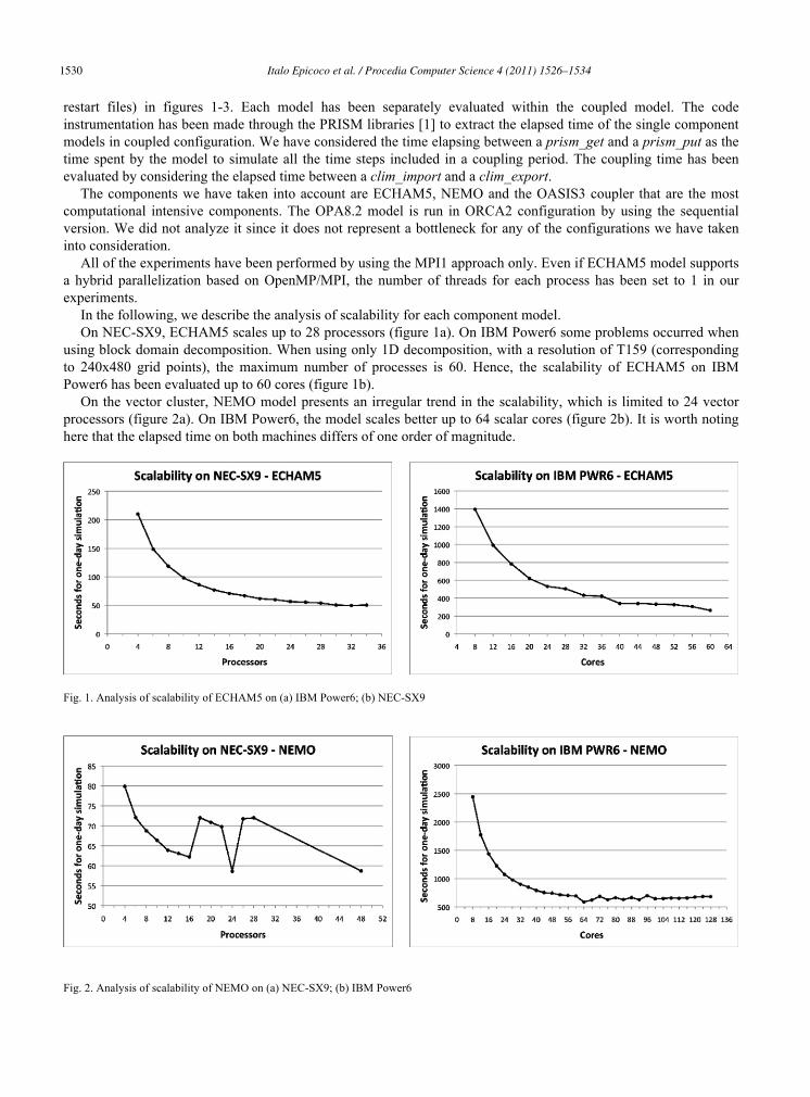
In the following, we describe the analysis of scalability for each component model. On NEC-SX9, ECHAM5 scales up to 28 processors (figure 1a). On IBM Power6 some problems occurred when

using block domain decomposition. When using only 1D decomposition, with a resolution of T159 (corresponding to 240x480 grid points), the maximum number of processes is 60. Hence, the scalability of ECHAM5 on IBM Power6 has been evaluated up to 60 cores (figure 1b).

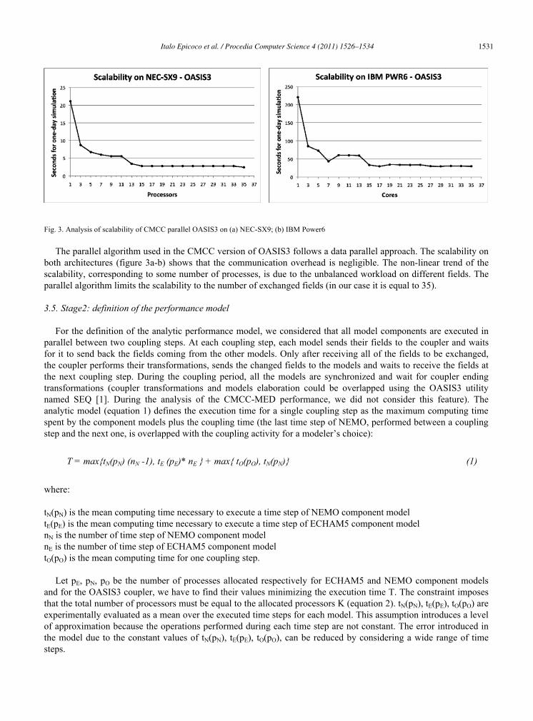
On the vector cluster, NEMO model presents an irregular trend in the scalability, which is limited to 24 vector processors (figure 2a). On IBM Power6, the model scales better up to 64 scalar cores (figure 2b). It is worth noting here that the elapsed time on both machines differs of one order of magnitude.

Fig. 1. Analysis of scalability of ECHAM5 on (a) IBM Power6; (b) NEC-SX9

Fig. 2. Analysis of scalability of NEMO on (a) NEC-SX9; (b) IBM Power6


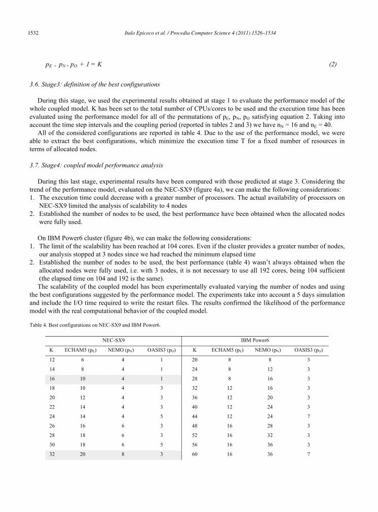
Fig. 3. Analysis of scalability of CMCC parallel OASIS3 on (a) NEC-SX9; (b) IBM Power6

The parallel algorithm used in the CMCC version of OASIS3 follows a data parallel approach. The scalability on both architectures (figure 3a-b) shows that the communication overhead is negligible. The non-linear trend of the scalability, corresponding to some number of processes, is due to the unbalanced workload on different fields. The parallel algorithm limits the scalability to the number of exchanged fields (in our case it is equal to 35).

3.5. Stage2: definition of the performance model

For the definition of the analytic performance model, we considered that all model components are executed in parallel between two coupling steps. At each coupling step, each model sends their fields to the coupler and waits for it to send back the fields coming from the other models. Only after receiving all of the fields to be exchanged, the coupler performs their transformations, sends the changed fields to the models and waits to receive the fields at the next coupling step. During the coupling period, all the models are synchronized and wait for coupler ending transformations (coupler transformations and models elaboration could be overlapped using the OASIS3 utility named SEQ [1]. During the analysis of the CMCC-MED performance, we did not consider this feature). The analytic model (equation 1) defines the execution time for a single coupling step as the maximum computing time spent by the component models plus the coupling time (the last time step of NEMO, performed between a coupling step and the next one, is overlapped with the coupling activity for a modeler’s choice):

T = max{tN(pN) (nN -1), tE (pE)* nE } + max{ tO(pO), tN(pN)} (1)

where: tN(pN) is the mean computing time necessary to execute a time step of NEMO component model tE(pE) is the mean computing time necessary to execute a time step of ECHAM5 component model nN is the number of time step of NEMO component model nE is the number of time step of ECHAM5 component model tO(pO) is the mean computing time for one coupling step.

Let pE, pN, pO be the number of processes allocated respectively for ECHAM5 and NEMO component models and for the OASIS3 coupler, we have to find their values minimizing the execution time T. The constraint imposes that the total number of processors must be equal to the allocated processors K (equation 2). tN(pN), tE(pE), tO(pO) are experimentally evaluated as a mean over the executed time steps for each model. This assumption introduces a level of approximation because the operations performed during each time step are not constant. The error introduced in the model due to the constant values of tN(pN), tE(pE), tO(pO), can be reduced by considering a wide range of time steps.


pE + pN + pO + 1 = K (2)

3.6. Stage3: definition of the best configurations

During this stage, we used the experimental results obtained at stage 1 to evaluate the performance model of the whole coupled model. K has been set to the total number of CPUs/cores to be used and the execution time has been evaluated using the performance model for all of the permutations of pE, pN, pO satisfying equation 2. Taking into account the time step intervals and the coupling period (reported in tables 2 and 3) we have nN = 16 and nE = 40.

All of the considered configurations are reported in table 4. Due to the use of the performance model, we were able to extract the best configurations, which minimize the execution time T for a fixed number of resources in terms of allocated nodes.

3.7. Stage4: coupled model performance analysis

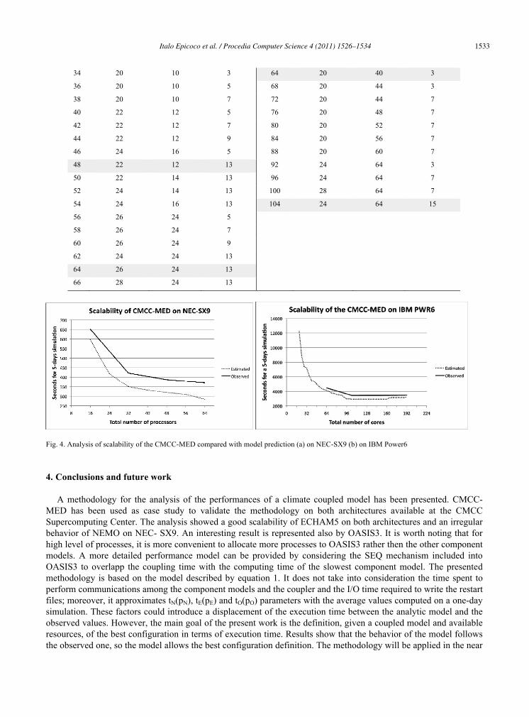
During this last stage, experimental results have been compared with those predicted at stage 3. Considering the trend of the performance model, evaluated on the NEC-SX9 (figure 4a), we can make the following considerations: 1. The execution time could decrease with a greater number of processors. The actual availability of processors on

NEC-SX9 limited the analysis of scalability to 4 nodes 2. Established the number of nodes to be used, the best performance have been obtained when the allocated nodes

were fully used.

On IBM Power6 cluster (figure 4b), we can make the following considerations: 1. The limit of the scalability has been reached at 104 cores. Even if the cluster provides a greater number of nodes,

our analysis stopped at 3 nodes since we had reached the minimum elapsed time 2. Established the number of nodes to be used, the best performance (table 4) wasn’t always obtained when the

allocated nodes were fully used, i.e. with 3 nodes, it is not necessary to use all 192 cores, being 104 sufficient (the elapsed time on 104 and 192 is the same). The scalability of the coupled model has been experimentally evaluated varying the number of nodes and using

the best configurations suggested by the performance model. The experiments take into account a 5 days simulation and include the I/O time required to write the restart files. The results confirmed the likelihood of the performance model with the real computational behavior of the coupled model.

Table 4. Best configurations on NEC-SX9 and IBM Power6.

NEC-SX9 IBM Power6

K ECHAM5 (pE) NEMO (pN) OASIS3 (pO) K ECHAM5 (pE) NEMO (pN) OASIS3 (pO)

12 6 4 1 20 8 8 3

14 8 4 1 24 8 12 3

16 10 4 1 28 8 16 3

18 10 4 3 32 12 16 3

20 12 4 3 36 12 20 3

22 14 4 3 40 12 24 3

24 14 4 5 44 12 24 7

26 16 6 3 48 16 28 3

28 18 6 3 52 16 32 3

30 18 6 5 56 16 36 3

32 20 8 3 60 16 36 7


34 20 10 3 64 20 40 3

36 20 10 5 68 20 44 3

38 20 10 7 72 20 44 7

40 22 12 5 76 20 48 7

42 22 12 7 80 20 52 7

44 22 12 9 84 20 56 7

46 24 16 5 88 20 60 7

48 22 12 13 92 24 64 3

50 22 14 13 96 24 64 7

52 24 14 13 100 28 64 7

54 24 16 13 104 24 64 15

56 26 24 5

58 26 24 7

60 26 24 9

62 24 24 13

64 26 24 13

66 28 24 13

Fig. 4. Analysis of scalability of the CMCC-MED compared with model prediction (a) on NEC-SX9 (b) on IBM Power6

4. Conclusions and future work

A methodology for the analysis of the performances of a climate coupled model has been presented. CMCC-MED has been used as case study to validate the methodology on both architectures available at the CMCC Supercomputing Center. The analysis showed a good scalability of ECHAM5 on both architectures and an irregular behavior of NEMO on NEC- SX9. An interesting result is represented also by OASIS3. It is worth noting that for high level of processes, it is more convenient to allocate more processes to OASIS3 rather then the other component models. A more detailed performance model can be provided by considering the SEQ mechanism included into OASIS3 to overlapp the coupling time with the computing time of the slowest component model. The presented methodology is based on the model described by equation 1. It does not take into consideration the time spent to perform communications among the component models and the coupler and the I/O time required to write the restart files; moreover, it approximates tN(pN), tE(pE) and tO(pO) parameters with the average values computed on a one-day simulation. These factors could introduce a displacement of the execution time between the analytic model and the observed values. However, the main goal of the present work is the definition, given a coupled model and available resources, of the best configuration in terms of execution time. Results show that the behavior of the model follows the observed one, so the model allows the best configuration definition. The methodology will be applied in the near


future also to other coupled models currently used at the CMCC.

References

1. S. Valcke and E. Guilyardi. On a revised ocean-atmosphere physical coupling interface and about technical coupling software. Proceedings of the ECMWF Workshop on Ocean-Atmosphere Interactions, Reading UK, 2008

2. I. Foster, J. Geisler, S. Tuecke and C. Kesselman. Multimethod communication for high-performance metacomputing. Proceedings of ACM/IEEE Supercomputing, Pittsburgh, PA, pages 1–10, 1997

3. V. Balaji, A. da Silva, M. Suarez et al. Future Directions for the Earth System Modeling Framework. White paper (http://www.earthsystemmodeling.org/publications/paper_0409_vision.pdf)

4. C. Hill, C. De Luca, V. Balaji, M. Suarez and A. da Silva. Architecture of the Earth System Modeling Framework. Computing in Science and Engineering, Volume 6, Number 1, pp. 18-28, 2004

5. S. Gualdi, E. Scoccimarro, A. Bellucci, P. Oddo, A. Sanna, P.G. Fogli et al. Regional climate simulations with a global high resolution coupled model: the Euro-Mediterranean case, 2010

6. S. Gualdi, E. Scoccimarro and A. Navarra. Changes in Tropical Cyclone Activity due to Global Warming: Results from a High-Resolution Coupled General Circulation Model. J. of Clim., 21, 5204–5228, 2008

7. E. Roeckner, R. Brokopf, M. Esch, M. Giorgetta, S. Hagemann, L. Korn-blueh et al. The atmospheric general circulation model echam5. Technical Report 354, Max Planck Institute (MPI), 2004

8. G. Madec, P. Delecluse, M. Imbard and C. Levy. Opa 8.1 ocean general circulation model reference manual. Technical report, Institut Pierre-Simon Laplace (IPSL), 1998

9. G. Madec. Nemo ocean engine. Technical Report 27 ISSN No 1288-1619, Institut Pierre-Simon Laplace (IPSL), 2008 10. M. Tonani, N. Pinardi, S. Dobricic, I. Pujol and C. Fratianni. A high-resolution free-surface model of the Mediterranean Sea, Ocean

Science, Ocean Sci., 4, 1–14, 2008 11. I. Epicoco, S. Mocavero and G. Aloisio. Experience on the parallelization of the OASIS3 coupler, Proceedings of 8th Australasian

Symposium on Parallel and Distributed Computing (AusPDC 2010) in conjunction with Australasian Computer Science Week, 18-22 January 2010

Documents

A Performance Evaluation Method for Climate Coupled Models