r.:a United States : ]l Department of · · Agriculture

Forest Service

Rocky Mountain Forest and Range Experiment Station

Fort Collins Colorado 80526

Research Paper RM-RP-319

A Pebble Count Procedure for Assessing Watershed Cumulative Effects

Gregory 5. Bevenger

Rudy M. King

This file was created by scanning the printed publication.Errors identified by the software have been corrected;

however, some errors may remain.

Bevenger, Gregory S.; King, Rudy M. A pebble count procedure for assessing watershed cumulative effects. Res. Pap. RM-RP-319. Fort Collins, CO: U.S. Department of Agriculture, Forest Service, Rocky Mountain Forest and Range Experiment Station. 17 p.

Abstract

Land management activities can result in the delivery of fine sediment to streams. Over time, such delivery can lead to cumulative impacts to the aquatic ecosystem. Because numerous laws require Federal land managers to analyze watershed cumulative effects, field personnel need simple monitoring procedures that can be used directly and consistently. One approach to such monitoring is described. The approach involves sampling a longitudinal reach of stream channel several hundred feet long using a zig-zag pebble count procedure that crosses all habitat features within a stream channel. The approach accommodates reference (unimpacted) and study (impacted) reaches so that impact comparisons can be made. Case studies show how the procedure is applied.

Keywords: Watershed cumulative effects, monitoring, watershed field techniques, pebble counts, sample sizes

The Authors

Gregory S. Bevenger is a hydrologist with the Shoshone National Forest, Cody, Wyoming. He graduated from Utah State University in 7978 with a B.S. in Forestry. Greg provides technical consultation on land management projects that affect soil and water resources.

Rudy M. King is Station Biometrician, Rocky Mountain Forest and Range Experiment Station, Fort Collins, Colorado. He has been a member of the Station's Biometrics Unit since 7977 and holds a M.S. in Mathematical Statistics from Colorado State University. Rudy provides statistical consultation for Station scientists and cooperators.

USDA Forest Service Research Paper RM-RP-319

A Pebble Count Procedure for Assessing Watershed

Cumulative Effects

Gregory S. Bevenger, Hydrologist

Shoshone National Forest1

Rudy M. King, Station Biometrician

Rocky Mountain Forest and Range Experiment Station2

'Forest Supervisor's Office is in Cody, Wyoming.

2Headquarters is in Fort Collins, in cooperation with Colorado State University.

May 1995

Contents Page

Introduction . . . . . . . . . . . . . . . . . . . . . . . . . . . . . . . . . . . . . . . . . . . . . . . . . . 1

Preliminary Sampling and Analysis.............................. 1

Validation Efforts . . . . . . . . . . . . . . . . . . . . . . . . . . . . . . . . . . . . . . . . . . . . . . 3

How to Use the Zig-Zag Pebble Count Procedure.................. 6

Using the Procedure in a Watershed Assessment ................. : 10

Conclusions .................................................. 13

Literature Cited ............................................... 13

Appendix 1. Statistical Framework .............................. 15

Appendix 2. Sample Size Estimation ............................. 16

A Pebble Count Procedure for Assessing Watershed Cumulative Effects

Gregory S. Bevenger and Rudy M. King

Introduction

Of concern in many National Forest watersheds is the cumulative effect of land management. One as­pect of this concern is the delivery of fine sediment to streams and its effect on aquatic habitat, particu­larly within pool and riffle complexes. To this end, the Clean Water Act requires the control of non-point sources of pollution through application of Best Man­agement Practices. To evaluate the effectiveness of such controls, stream monitoring needs to occur. The most desirable form of monitoring is one that is rela­tively simple to implement, can be used directly and consistently by field personnel, and is sensitive enough to provide a measure of impact. Ideally, in­dices of sediment in streams can be obtained by mea­suring channel substrate material in comparison to reference streams, where little or no management has occurred.

We have developed a field procedure for charac­terizing particle size distributions of reference and study streams, where we define reference streams as "natural" or "unimpacted" and study streams as "disturbed" or "impacted." These distributions can be used for comparative purposes to determine, with statistical reliability, if there has been a shift toward finer size material (fine gravels to sands) in the study stream. Knowledge of such a shift is important be­cause increases in this size material can negatively impact the aquatic ecosystem (Meehan 1991; MacDonald et al. 1991). If monitoring demonstrates that a shift toward finer size material has or is taking place, corrective actions can be taken within either (1) the watershed to reduce the amount of sediment being delivered to the stream or (2) the stream itself to remove the introduced sediment.

Wolman (1954) described a method for sampling coarse riverbed material that is rapid and produces statistically reliable information on the median bed particle size. His procedure involves randomly sam­pling bed material within a grid system and then plotting these data as a cumulative frequency distri­bution. His method is commonly modified by estab­lishing transects across the channel (cross-sections

perpendicular to the flow) and sampling on a toe-to­heel spacing until1 00 pebbles within habitat features of interest (pools, riffles, or combinations thereof) are collected (Leopold 1970).

Our interest is in shifts in the fine gravel and smaller portion of the distribution, not the median. Therefore, through a longitudinal stream reach (most commonly a pool and riffle complex) we modified the Wolman procedure into a zig-zag pattern such that a stream reach is sampled along a continuum instead of an individual cross-section. By doing this, numerous meander bends and all associated habitat features can be sampled as an integrated unit rather than as individual cross-sections.

Preliminary Sampling and Analysis

In 1992, we conducted preliminary sampling and analysis to determine if the zig-zag procedure was worth pursuing in detail. Many reference and study reaches within the headwaters of the Clarks Fork of the Yellowstone River drainage were sampled. We located four stream classes within these watersheds that have characteristics common to both reference and study reaches of immediate interest. The classes are based on a stream classification hierarchy devel­oped for the Shoshone National Forest (Hoskins 1979) that integrates gradient, watershed area, landform, lithology, and channel pattern as differentiating char­acteristics. Of the 37 classes identified by Hoskins, we limited sampling to classes 3, 5, 10, and 16. Class 5 reference reaches were sampled in anticipation of future needs even though no study reaches having this class were present in the sampled watersheds. Table 1 displays the characteristics of these particu­lar stream classes.

From topographic maps that showed the stream class delineations, individual reaches to be sampled were located in the field. Then we followed a zig-zag pattern of going upstream from bankfull to bankfull (as illustrated in figure 1 and explained in more de­tail later) and measured pebbles at approximately 7 -foot intervals. One hundred pebbles were mea-

Figure 1.- bble coun Zig-zag pe

2

t Procedure.

Table 1.- Stream classes used in this study and their characteristics.

Stream class Stream gradient Watershed area

3 6-12% <4mi2

5 3-6% <4mi2

10 3-6% 4-20 mF

16 2-3% 4-20 mi2

sured within each reach, which translated to sam­pling a longitudinal profile several hundred feet long. Pebbles were randomly selected by reaching over the toe of the wader with an extended forefinger and picking up the first rock that was touched. The inter­mediate axis of each selected pebble was measured and tallied using standard Wentworth size classes (particles less than 2 mm; 2-4 mm; 4-8 mm; 8-16 mm; 16-32 mm; 32-64 mm; 64-128 mm; 128-256 mm; 256-512 mm; 512-1,024 mm; 1,024-2,048 mm; and 2,048-4,096 mm). Figure 2 displays particle size distribu­tions for reference streams sampled in 1992, while figure 3 displays distributions for study streams.

These data were analyzed using contingency tables (gross Wentworth size classes of sands, gravels, cobbles, and boulders as columns and different reaches as rows) and the Pearson chi-squared statis­tic. Comparing reaches within classes, particle size distributions were homogeneous for class 5 and larger (p>0.13). Within class 3, particle size distribu­tions were heterogeneous (p<0.001), but large differ­ences were present only for cobble and boulder size classes. When particle sizes were summarized as pro­portion of fine particles and proportion of larger par­ticles, no differences were present among reference reaches across all classes and using a variety of cut­off points <8mm to define fine particles (p>0.68). We concluded that reference particle size distributions are relatively homogeneous for smaller size classes (fine gravels and smaller) and that study reach par­ticle size distributions are significantly different from reference distributions (p<0.001). This finding en­couraged us to pursue a more rigorous analysis of the proposed procedure.

Validation Efforts

Using the results of the previously described pre­liminary effort in concert with several specific prag­matic assumptions, a statistical framework was de-

3

Landform Lithology Channel pattern

Not defined Volcanic Not defined

Not defined Volcanic Not defined

Alluvium Volcanic Not defined

Alluvium Volcanic Not defined

signed so the zig-zag pebble count procedure could be validated. This framework is described in detail in Appendix 1. Within this framework, additional field data were collected in 1993 and subjected to comprehensive statistical analysis.

The generic null hypothesis for the validation ef­fort is the population of pebbles from the reference condition and the population of pebbles from the study condition are the same. This hypothesis re­quires testing several assumptions: (1) individual pebbles in a sample are independent members of the appropriate target population; (2) location of sample points within a stream reach is unimportant; (3) data from multiple reference stream reaches can be com­bined to appropriately represent a reference popula­tion (condition); and (4) sample results are indepen­dent of the field observer.

Each of these assumptions was analyzed by per­forming additional pebble counts in 16 reference reaches within 2 of the same streams sampled in 1992, Republic and Closed Creeks. As noted earlier, these reaches have similar lithology (volcanic) and a speci­fied range of drainage area and gradient. Each reach was sampled by the senior author and one of three other observers. Each observer sampled 300 pebbles in each reach in Republic Creek and 200 pebbles in each reach in Closed Creek. Distance between samples was approximately 3.5 feet in all cases. Pebble size was recorded to the nearest millimeter to permit detailed analysis of the particle size distribution.

Assumption 1: Independence of Pebbles To analyze independence of pebbles within a

sample, autocorrelations of up to 20 lags were esti­mated for the senior author's data (to control for any variation among observers) for each reach. Auto­correlation is defined as the correlation between pairs of sequentially observed points (Chatfield 1989). Lag 1 autocorrelation (or serial correlation, r1) is the cor­relation between each pair of adjacent points; lag 2

autocorrelation (r 2) is the correlation between every other point; lag 3 autocorrelation (r3) is the correla­tion between every third point; and so on. Lag 1 auto­correlations on 2 of the 16 reaches were 0.26 and 0.43, respectively, and these were significant at a=O.OS. Typi­cal values for r 1 ranged from 0.10 to 0.20. Auto­correlations at longer lags, r2 to r20' were not significant for any reach. In summary, there was occasionally a worrisome level of correlation between pebbles sampled 3.5 feet apart; there was never significant cor­relation between pebbles sampled at least 7 feet apart.

Assumption 2: Sampling Location Unimportant To analyze the importance of sampling location

within a reach, the senior author's data (again, to control for any observer variation) were divided into 2 (Closed Creek) or 3 (Republic Creek) 100-point sub-reaches. Sub-reaches within each reach were

Stream Class 3 100

c .... > ro I/ v £ 80 <u // c

I+= 60 _. I

::R 0

Q)

> 40 ~ 'i :::::! /if E 20 :::::! ~v u F,i.>

0 -r:-1 10 100 1000 10000

Particle size (mm)

Stream Class 10 100 -···· ...

c '~./~ -

ro £ 80 ./

<u / 1/'

c <:/ I+= 60 ::R .. [/ 0

Q)

> 40 ~ .. I/

:::::! --~

_,;;/

E 20 / :::::! ??' u -

~ 0····

0 1 10 100 1000 10000

Particle size (mm)

c ro £ <u c

I+=

::R 0

Q)

> § :::::!

E :::::! u

c ro £ <u c

I+=

::R 0

Q)

> § :::::!

E :::::! u

compared using contingency tables structured to: (1) divide particle sizes into gross Wentworth size classes of sands, gravels, cobbles, and boulders and (2) di­vide particles into ::;;4 mm vs. >4 mm; ::;;6 mm vs. >6 mm; ::;;s mm vs. >8 mm; and ::;;10 mm vs. >10 mm. These latter divisions were made to represent vari­ous definitions of sediment that might be defined as biologically significant. Only 2 reaches exhibited sig­nificant (a=O.OS) differences between the sub-reaches; one reach for the gross Wentworth size classes and one reach for the 10 mm cutoff point. In general, within-reach variability was minor.

Assumption 3: Multiple Stream Reaches Can Be Combined to Define a Reference

The reference condition must be well-defined to assume that a study reach would be the same as the reference condition if not impacted. Otherwise a null

Stream Class 5 100

80

60

-r· 1--..-·

/~ /·/

40 /.··

20 /. .. :: ....

-?•"

0 f-:-::::-. ~-·

1 10 100 1000 10000 Particle size (mm)

Stream Cl2ss 16 100

80

60

I ~~--

I 40

v

20 /1 v ..... / -

0 -~='

1 10 100 1000 10000 Particle size (mm)

Figure 2.- Particle size distributions of reference streams sampled in 1992. Different lines refer to different reaches.

4

hypothesis that reference and study streams are not different would not be tenable. This suggests one should define a reference population·using as many reference reaches as possible and use this as the ba­sis for comparing impacted reaches.

To analyze this assumption, we explored the ques­tion, "To what degree are particle size distributions homogeneous among reference reaches?" The senior author's data was (1) compared among reference reaches within and between creeks (Republic and Closed Creeks) for 4 individual stream classes (Shoshone stream classes 3, 5, 10, and 16) using con­tingency tables and (2) compared between creeks and among stream classes using log linear models. Log linear models allow for frequency analysis of more than the two factors analyzed in a contingency table (see Agresti 1990). Particle size distributions were characterized as before using both gross Wentworth

Stream Class 3 100 f;-"""'.·

....... -

~ c

~ ro I

:5 80 VI

.....

m VI ........ c I;: 60 ....

/ ...... ":§?. 0 v Q)

> 40 :.;:; / v ro / ~ :::J

E 20 :::J ~f-

0 0

1 10 100 1000 10000 Particle size (mm)

size classes (sands, gravels, cobbles, and boulders) and "small" and "large" particles as defined by vari­ous cutoff points (4, 6, 8, and 10 mm).

For individual stream classes, comparisons of stan­dard size fractions between creeks were significant for stream classes 10 and 16 (significance levels are displayed in table 2a), with differences apparent only for gravel and larger material. Similar comparisons assuming the various cutoff points of 4, 6, 8, and 10 mm were significant only for stream class 3 (table 2a). When multiple stream classes were added to the analysis using log linear models: heterogeneity among stream classes was evident. Additionally, stream class 3 exhibited evidence of internal heterogeneity (table 2b).

In summary, for the cutoff points used, reaches in individual stream classes 5, 10, and 16, both within and between Republic and Closed Creek, were ho­mogeneous. Class 3 pooling attempts, both within

Stream Class 10 100

.J~ b"~ c v

ro ·If :5 80 ,' I I... "/ Q) ..... c /

it= 60 ;:R ......... 0 //

_..; /, / Q)

> 40 ~

~~ p.· -- ,..;~

:::J

E 20 :::J 0

0 1 10 100 1000 10000

Particle size (mm)

Stream Class 16

c ro :E 03 c it=

;:R 0

Q)

> ~ :::J

E :::J (.)

100

80

60

40

20

0 1

/

v /

v -~

10 100 1000 10000 Particle size (mm)

Figure 3.-Particle size distributions of study streams sampled in 1992. Different lines refer to different reaches.

5

and between Republic and Closed Creek, exhibited heterogeneity. This was considered in the compari­son of class 3 reference conditions to a study reach (e.g., Case Study 2later in this paper). Pooling reaches among stream classes was not successful.

Assumption 4: Independent of Field Observer The fourth assumption tested was whether sample

results are independent of field observer. Data from the two observers for each reach were compared us­ing contingency tables structured similar to those ~sed ~or as~es~ing. sampling location. When the par­ticle size distnbution was characterized using gross Wentworth size classes (sands, gravels, cobbles, and boulders), 7 of 10 reaches for Republic Creek and 5 of 6 reaches for Closed Creek showed significant dif­ferences (a=O.OS) between the data collected by the s~nior author and the second observer. When par­ticles were divided into "small" and "large" classes as defined by the various cutoff points of 4, 6, 8, and 10 mm used in previous analyses, 3 of 10 reaches for Republic Creek showed significant differences; no significant differences were present for Closed Creek. The improved agreement between observers for Clos~d c:=reek may be due to increased training and monitonng of the second observer while sampling. However, second observers were different between Republic and Closed Creek, so a conclusive statement cannot be made from these data. Regardless, where observer variability was present, it was more severe for larger particle sizes (cobbles and boulders). This may be because cobbles and boulders are difficult to measure to the nearest millimeter or because there is inherent wide variability in cobble and boulder size :naterial. In co.nclusion, data should be analyzed us­Ing cutoff points of interest rather than by gross Wentworth size classes.

How to Use the Zig-Zag Pebble Count Procedure

Step 1. Think about how to delineate reference and study reaches. We used the Shoshone stream classi­fication system. Other stream classification systems may work just as well. Classifying reaches by water­shed area, gradient, and lithology may be sufficient. Whatever delineation technique is used, you should conduct preliminary sampling and analysis to deter­~ine if the effort i~ worth pursuing. It is particularly Important to stratify reference reaches into homoge­neous groups. When this cannot be accomplished (e.g., as was the case for class 3 reaches on the Sho­shone National Forest), the analysis should reflect the heterogeneity of the reference condition (e.g., Case Study 2 later in this paper).

Before initiating field work, you should ask, "How many pebble counts are needed to detect a real dif­ference between reference and study conditions?" To answer this question, the nature of the reference con­dition, the size of change that might occur from a management action, and acceptable levels of risk must be sp~cified. Discussion of this analysis is post­poned until Step 4 below to allow a direct link to be made with the statistical analysis, but it should be completed before Step 2.

Step 2. Delineate reference and study reaches on topographic maps, and then locate the reaches in the field. _figure 1 illustrates the basic zig-zag sampling technique. For each reach, choose a random location on one bank at bankfull stage. Once you locate this poi~t, identify an upstream target point on the op­posite bank that can be used to hold a straight line while sampling. Then pace off 7 feet (3 to 4 steps de­pending on your pace), reach over the toe of the

Table 2a.-Significance levels of contingency table comparisons between Republic and Closed creeks for reference data collected by Bevenger.

Small vs. large particles greater than:

Stream class Standard fractions 10mm 8mm 6mm 4mm 2mm

3 0.469 0.018 0.004 0.021 0.088 0.124

5 0.096 0.292 0.573 0.760 0.932 0.685

10 <0.001 0.239 0.142 0.172 0.485 0.999

16 0.019 0.444 0.481 0.416 0.958 0.999

6

Table 2b.-Significance levels of log linear model components1 for comparisons between Republic and Closed Creeks and among stream classes for reference data collected by Bevenger.

Small vs. large particles greater than:

Model components Standard fractions lOmm 8mm 6mm 4mm 2mm

1st order <0.001 <0.001 <0.001 <0.001 <0.001 <0.001

2nd order <0.001 <0.001 <0.001 <0.001 0.001 0.003

3rd order 0.039 0.075 0.031 0.071 0.367 0.366

1 1st order factors are particle size class, stream class, and creek. 2nd order components are interactions between 2 of the factors. The 3rd order component is interaction among all 3 factors.

wader with the forefinger without looking down, pick up the first pebble touched, and measure it in millimeters. If it is less than 64 mm, record the actual size on the data form (figure 4 contains a sample form). If it is greater than or equal to 64 mm, assign the sample to the appropriate Wentworth size class by recording the class midpoint based on a log scale:

91 for pebbles 64-127 mm; 182 for pebbles 128-255 mm; 363 for pebbles 256-511 mm; 724 for pebbles 512-1,023 mm;

1,445 for pebbles 1,024-2,047 mm; and 2,884 for pebbles 2,048-4,095 mm. This recording method allows for analysis of cut­

off points such as 4, 6, 8, and 10 mm as well as other types of pebble count applications as mentioned in the introduction. Once you record the pebble, dis­card it, focus on the target, pace 7 feet, and sample another pebble. Continue working across and up the stream until you reach the far bankfull. Then locate another target, this time on the bank on which the survey line began, and work across the creek. Con­tinue this technique until the desired number of pebbles are sampled.

The result should be a zig-zag line that traverses through a stream reach such that somewhere along the zig-zag the inside and outside of riffles, runs, pools, and meander bends are sampled. The angle of the zig-zag depends upon the meander pattern of the stream reach being sampled. We cannot give pre­cise instructions on what the angle of the zig-zags should be except that low sinuosity reaches require less sharp angles than high sinuosity reaches. If chan­nellength is defined as the distance along the thalweg (i.e., deepest point of the channel), and if the sam­pling design called for 100 pebbles at 7-foot inter­vals, then 700 feet of stream reach would be sampled

7

if all samples were taken from the thalweg. Since the zag-zag pattern follows a bankfull to bankfull line across and up the channel, less than 700 feet of thalweg length will actually be sampled. Our field experience indicates that the ratio of zig-zag length to thalweg length ranges from 0.85 to 0.95. In other words, our final reach lengths were between 595 and 665 feet, instead of 700 feet. Of course, these ratios hold only for the streams we sampled. Streams of different sinuosity would have different ratios.

Individuals should be trained before starting field sampling and regularly monitored while sampling to ensure they are properly applying the technique. We found that poorly or improperly trained people collected data significantly different from that col­lected by trained people. Additional training rem­edied this. Important factors to consider and moni­tor during training are that (1) spacing between pebble samples is correct, (2) pebbles are being selected properly, (3) pebbles are being measured properly, and (4) the zig-zag pattern is being properly laid out.

Step 3. Randomly choose several streams (and reaches within streams) from those available in a class to define the variability within the reference condi­tion. Reaches within each hypothesized reference condition should be analyzed for homogeneity, and subsequent analyses should reflect any heterogene­ity found (e.g., class 3 reference reaches and Case Study 2 below). If a rationale can be found and suffi­cient data exists, it may be possible to further stratify heterogeneous reference conditions into homoge­neous subsets. However, sufficient data should be obtained to precisely describe each subset for subse­quent comparison to study reaches. The intensity of sampling needed to define each reference condition and study reach is discussed in Step 4.

Str

ea

m:

Par

ty:

Da

te:

Cla

ss:

Se

gm

en

t:

Up

pe

r M

idd

le

Lo

we

r

Siz

e: 1

<2

mm

; 2

mm

<a

ctu

al>

63

mm

; 64

<91

>12

7; 1

28<

182>

255;

256

<36

3>51

1; 5

12

<7

24

>1

02

3;

1024

<14

45>

2047

; 20

48<

2884

>40

95.

# S

ize

#

Siz

e

# S

ize

#

Siz

e

# S

ize

#

Siz

e

# S

ize

1

46

91

136

181

226

271

2 47

92

13

7 18

2 22

7 27

2 3

48

93

138

183

228

273

4 49

94

13

9 18

4 22

9 27

4 5

50

95

140

185

230

275

6 51

96

14

1 18

6 23

1 27

6 7

52

97

142

187

232

277

8 53

98

14

3 18

8 23

3 27

8 9

54

99

144

189

234

279

10

55

100

145

190

235

280

11

56

101

146

191

236

281

12

57

102

147

192

237

282

13

58

103

148

193

238

283

14

59

104

149

194

239

284

15

60

105

150

195

240

285

16

61

106

151

196

241

286

17

62

107

152

197

242

287

18

63

108

153

198

243

288

19

64

109

154

199

244

289

20

65

110

155

200

245

290

CX>

21

66

111

156

201

246

291

22

67

112

157

202

247

292

23

68

113

158

203

248

293

24

69

114

159

204

249

294

25

70

115

160

205

250

295

26

71

116

161

206

251

296

27

72

117

162

207

252

297

28

73

118

163

208

253

298

29

74

119

164

209

254

299

30

75

120

165

210

255

300

31

76

121

166

211

256

301

32

77

122

167

212

257

302

33

78

123

168

213

258

303

34

79

124

169

214

259

304

35

80

125

170

215

260

305

36

81

126

171

216

261

306

37

82

127

172

217

262

307

38

83

128

173

218

263

308

39

84

129

174

219

264

309

40

85

130

175

220

265

310

41

86

131

176

221

266

311

42

87

132

177

222

267

312

43

88

133

178

223

268

313

44

89

134

179

224

269

314

45

90

135

180

225

270

315

..

Fig

ure

4.-

Fie

ld d

ata

form

.

Based on the analyses that we performed and con­sidering that only two streams were available for comparison, reaches of similar Shoshone stream class could be pooled both within and between streams to describe a reference condition involving small par­ticle sizes. Reaches cannot be pooled among differ­ent stream classes, and describing a reference condi­tion for larger particle sizes seems problematic. For similar Shoshone stream classes, the number of reaches used to describe a reference condition should increase as the spatial scale of the reference condi­tion increases.

Step 4. The hypothesis recommended for testing is

H 0 : Ps- Pr = 0 versus Ha: Ps- Pr > 0

where Pr is the reference proportion (for instance, the proportion of fines <8mm) and Psis the respective proportion for a study condition. This is a test where detection of a significant increase on the study condi­tion is all that is considered important (that is, in sta­tistical terms a one-tailed test is being used). As noted in Step 1, you should answer the question "How many pebble counts are needed to detect a real dif­ference between reference and study conditions?" before initiating field work. Fleiss (1981) shows how to estimate needed sample sizes, both when equal sample sizes are used for the two conditions (equa­tions 3.14 and 3.15) and when unequal sample sizes are used (equations 3.18 and 3.19). Fleiss's equations are provided in Appendix 2 for use in situations that require exact sample size calculations. Figures 5 and 6 plot various combinations of proportions and sample sizes for situations in which coarser estimates of needed sample sizes are sufficient.

To demonstrate use of the sample size graphs, as­sume there is a timber sale and associated road build­ing planned in a municipal water supply. The local sawmill may suffer economically if the sale does not occur, and the municipality will be impacted if the sale results in increased sedimentation in the water supply. A decision is made to use the zig-zag pebble count procedure as one tool in the analysis of the sale.

The potential costs associated with both Type I (a) and Type II (f3) errors should be considered when estimating sample sizes. A Type I error in the present example is the risk of falsely concluding that there is a difference between the study stream and its refer­ence, which might lead to a decision to postpone the sale. A Type II error in the present example is the

9

probability of falsely concluding there is no differ­ence between the study stream and its reference, which might lead to a decision to proceed with the sale as pro­posed, potentially resulting in increased water treatment costs. Typically, sample sizes are estimated assuming f3=4a, most commonly a=0.05 and f3=0.20 (Fleiss 1981).

The sample size question can be broken into two parts: (1) what sample size is needed to define the reference condition and (2) what sample size is needed to define the study reach? To answer these questions, the nature of the reference condition, the size of change that might occur from a management action, and the risk levels (a and f3) that are accept­able must be specified. Suppose no existing reference data are available, but you hypothesize that the pro­portion of particles <8 mm for the reference condi­tion is about Pr=0.10 and a change on the study reach to p

8=0.20 or larger (i.e., a change of 0.10 or larger) is

considered biologically significant. For standard values of a=0.05 and f3=0.20, the up­

per right graph in figure 5 shows sample sizes needed to detect a difference of Ps -pr>0.10. First, locate the difference point of 0.10 on the vertical axis and scan across the plot horizontally to the curve represent­ing the reference sample size. Then, read down to the horizontal axis to obtain the sample size needed for the study reach. For example, if a sample size of nr=450 or larger were used to characterize the refer­ence condition, then a sample size (n) of 100 or less would be needed for the study condition. If nr=300 were used to define the reference condition, n

8=115

would be needed for the study condition, while an nr=150 would require about n

8=215. Sample sizes

substantially larger than 300 would be required for the study condition if nr=100 were used for the refer­ence condition. Alternatively, if the minimum differ­ence considered biologically significant were relaxed to Ps -pr=0.15, then a sample size of 100 would be more than adequate for both reference and study conditions.

In some situations, such as if a threatened species were present, it might be appropriate to strike a bal­ance between both errors rather than worrying more about the risk of falsely declaring a difference. Fig­ure 6 contains plots of sample sizes needed when both a and f3 are set equal to 0.05. When Pr=0.10, de­tecting a difference of p

8-pr=0.10 would require about

n5=290 for nr=300. Increasing the sample size for the

reference condition to nr=450 or 600 would decrease the sample size needed for the study condition to about n

8=215 or 190, respectively.

After a point, increasing the sample size for the reference condition does not result in an equal re­d~~tion i~ the sample size needed for the study con­dition. This can be seen in both figures 5 and 6, where distance between reference lines decreases at larger reference condition sample sizes. The trade-off be­tween this and minimizing sample size for both con­ditions is that additional sampling will result in a better description of the reference condition that could be used for more than one study reach, each of which could be sampled with fewer samples. In gen­eral, we recommend sampling several reaches to characterize the range of variability of the reference condition with the side benefit that less sampling will be needed for comparing several study conditions to the same reference condition.

Reference proportion = 0.05 Q)

g 0.25 r-----:-------,-------,-----~ ~ Q)

1§ 0.2 +-----------------·----------+--------------------------- '- ---------------------Q)

::0 ~ 0.15 +--------------- --------------<-------------------------------<-------------------···--··· ····•----------------------------- I Q) +'

~ -... E 0.1 .............:=----------,--------- . -------------------------

:~0.05 ~ •...................................

~ . 100 150 200 250 300 Sample size for study condition

Reference proportion= 0.15 Q)

g 0.25 r-----:-------,-------,-----~ ~ Q)

1§ 0.2 +--------------------- --------i-------------------------------i- -- ------------------- ----- _, _____________________________ -I

Q)

::0 ~0.15 .........

~ ~.........::::~~ "'0 ~------E 0.1 ::J E -

:f:; 0.05 --'----'-~~__._________._~~~--'-~~~___i_~~__._j ~ 100 150 200 250 300

Sample size for study condition

Using the Procedure in a Watershed Assessment

A coarse screening process was recently developed on the Shoshone National Forest to analyze water­shed cumulative effects. This screening process re­vealed numerous watersheds of concern (Shoshone National Forest 1993). A watershed of concern is de­fined as a fourth-order drainage where inherent soil and water sensitivity plus land disturbing activities may be causing significant degradation of aquatic resources. In such watersheds any additional surface disturbance may only add to the level of concern. Since the effort was programmatic and the screens were coarse, managers required that a watershed of concern be field verified to determine if the water­shed and streams within it are actually in a degraded

Reference proportion= 0.10 Q) g 0.25 ,---------,--------,---------,----~ Q)

~ 0.2 t··---------------------------~--------------------------- i····-----------------------+-----------------------···----1 Q)

::0 ~ 0. 15 ±:······--·------------------·+·-----·-··-·----------------- <- ------------------------------~--------------------····· ..... 1 Q) --.......

Q) ~ "'C

~ 0.1 ~:::;:::::::: ... : ........... ,.: .... ::: .. -.':"

:f; 0.05 -'----'~~._____._~~~--'--~~.....___i~~~-_j ~ 100 150 200 250 300

Sample size for study condition

Reference proportion= 0.20 Q)

g 0.25 ,-------:-------,-------,-----­Q)

~ 0.2 t-----------------------------;-------------------------------'--·-·----·------------·---------''---·-····-·----------------------

~

~:-i-............. ,_j __

250 300 Sample size for study condition

-100 -150 ··--·- 300 -450 -600

Figure 5.-Minimum detectable difference and study condition sample size estimates assuming a = 0.05 and ~ = 0.20.

10

condition. After field verification, appropriate site-specific mitigation requirements could then be developed and implemented. Mitigation require­ments may be in the form of "standard operating procedures" if a watershed is not one of concern or in the form of "extraordinary mitigation" if the wa­tershed is one of concern.

Since pebble count data were available for both reference and study reaches, we used these data to demonstrate one part of the process of verifying the level of concern and amount of mitigation that would be needed if additional management were to take place. More specifically, contingency tables were es­tablished to compare small and large particle size fractions between reference and study reaches. We used the data collected in 1993 from Republic and

Reference proportion = 0.05

Q)

g 0.25 -..------,-----,.-------.,-----------, Q)

~ 0. 2 +······------·--·-------------~----··-------- ................ , ............................... , .......................... .. Q)

:c ~ 0.15 Q)

a> "C E 0.1 :::::J E :£ 0. 05 .l....-L~_.__,____,__..__~'--'-----'--~~~-'---->-_..__-'---'~

~ 100 150 200 250 300 Sample size for study condition

Reference proportion = 0.15 Q) g 0.25 ...---------,-----..,------,---------, Q)

~ 0.2 Q)

:c ~ 0.15 2 ··----~----..... ~ 0.1 L ........................ ..J=~===t~~~~;;;;;;;J :::::J E :~ 0.05 J___,~_.__....____._~_.__~__J_._.__~~.....L...-~~~ ::=:E 100 150 200 250 300

Sample size for study condition

Closed Creeks to represent reference reaches. For study reaches we used data collected from our ini­tial reconnaissance work conducted in 1992. MacDonald et al. (1991) summarize the literature by reporting that particles up to 6.4 mm are of most con­cern to the fishery resource. Since the 1992 data were collected by Wentworth size classes, we used <8 mm as the cutoff point because this is the size class clos­est to, but yet greater than or equal to, 6.4 mm. We are confident with our approach because we com­pared reaches that are similar in lithology, watershed area, and gradient as incorporated by the Shoshone stream classification system. The following four case studies briefly describe the results of these comparisons.

Reference proportion= 0.10

Q) g 0.25 ...--------,------:------:-----, Q)

~ 0.2 +---------------------·------+--------------------------··--r----·----------------·----·· Q)

::0 ~ 0.15 2 Q)

"C

E 0.1 :::::J E

...................... 1 ............................. :

-------------i--------------·:::.::::.::i:.:::.:::.-.-., .... ___ , __

:~ 0.05 .l....-L~_.__....__j,_~-~~-'--~~......__..~_.__~__, ::=:E 100 150 200 250 300

Sample size for study condition

Reference proportion = 0.20

Q)

g 0.25 ,--------,------:------:,-------, Q)

~ 0.2 Q)

:c ~ 0.15 Q) +-' Q)

"C E 0.1 :::::J E

•·•••u•••••-••••:••·•••••••••••• •••••••••••••-:-•••••••••••·••·•·

··-·-·····i····-- : --·--·-!-·--

:~ 0.05 ..L......~~...____J.,_..__~..........___.__..___,__..___._jl..___j__.__~__J

::=:E 100 150 200 250 Sample size for study condition

-100 -150 .... 300 -450 -600

300

Figure 6.-Minimum detectable difference and study condition sample size estimates assuming a = 0.05 and p = 0.05.

11

Case Study 1 : Recent Wildfire Lodgepole and Pilot Creeks were heavily burned

by the Clover-Mist Fire in 1988. Recovery of surface-protecting v~getation within both watersheds has been very slow and was practically nonexistent the first 2 years after the fire. The fire caused a con­siderable water yield increase that has resulted in major adjustments in stream channel morphology (Troendle and Bevenger 1993). Additionally, Lodge­pole Creek received a significant rainfall event the summer after the fire that resulted in exceptionally large amounts of overland flow, substantial changes in channel morphology, and considerable inner gorge mass movement activity. Figure 7 displays post-fire particle size distributions for a class 10 reach in both Lodgepole and Pilot Creeks versus the distribution for the class 10 reference. These 2 reaches are signifi­cantly different from the reference (significance level

100

80

60

40

20

0 1

Case Study 1 - Recent Wildfire

~ 1--

f---1~/

~r--

J llilll~ lll ~ r,

JJtil!l _ j r 1 : 1~

i i ; i

/

10

illL 1

!

100

Particle size (mm)

- - Lodgepole - Pilot

1000

-Reference

10000

Case Study 3 - Current Stock Grazing 100

80

60

40

20

0 1

-

i-1-

~ j----

~

l v?r ll / J I -

~+ 1/ I! ~t I_ J I I I

v /

/ Ill 'T

10

- -- Elk

100

Particle size (mm)

-Reference

1000

I i n -r~ , I

I ,

ll 10000

p<0.001 for both reaches) for particles less than 8 mm (p,=0.10 versus p

5=0.37 and p

5=0.28, respectively).

Case Study 2: Recent Timber Harvest Jim Smith Creek flows through an area that was

logged in the late 1980's. Trees were harvested along the banks of the creek. Due to the inherent instabil­ity of the channel, many of the root wads have since sloughed into the channel. Fine material surround­ing the root wads is being scoured by the streamflow and deposited downstream. Figure 7 displays the post-harvest particle size distribution for a class 3 study reach versus the distributions for the class 3 reference reaches. For particles less than 8 mm, this reach is significantly different from 2 of the reference reaches (p

5=0.22 versus p,=0.06 [p<0.001] and p,=0.11

[p=0.009]), but not the third (p,=0.14 [p=0.068]). Therefore, the small size fraction on Jim Smith Creek

Case Study 2 - Recent Timber Harvest 100

I II !

,-------,----r ~p

II I / c---

I 1(1

- r------ --80

60

~ I l ' ~~

I I

~ ~ ~~

/

40

20

0 1

t:# v~ /

10

,_ --

I I

100

Particle size (mm)

- c_

1000

- Reference 1 - - Reference 2 - - Reference 3 - Jim Smith

Case Study 4- Old Wildfire

Particle size (mm)

- - Gravelbar - - Huff --- Reference

I l

10000

Figure 7.-Particle size distributions of case study streams.

12

is comparable to the upper end of the variability ob­served in the reference condition, but quite different from the lower end of the reference variability. This suggests that before making mitigation recommen­dations in this situation further analysis is needed. Additional class 3 reference reaches could be sampled to establish a better estimate of the "norm" and thereby provide for a conclusive interpretation of the fine sediment load in Jim Smith Creek. Also, the log­ging effects analysis could be expanded by additional on-site assessment of other indicators of watershed condition and stream health.

Case Study 3: Current Stock Grazing Elk Creek flows through an active cattle grazing

allotment. Cattle congregate within the riparian zone, resulting in considerable trailing near the channel and sloughing of the banks. Figure 7 displays the current particle size distribution for a class 16 study reach versus the distribution for the class 16 refer­ence. The study reach is significantly different from the reference (p<0.001) for particles less than 8 mm (pr=0.08 versus p

8=0.39).

Case Study 4: Old Wildfire Gravelbar and Huff Gulch Creeks flow through an

area burned 50 years ago by the Gravelbar Fire. Slopes less than 50% have recovered quite well to grasses on south aspects and lodgepole pine on north aspects. Slopes steeper than 50% show minimal re­covery, probably due to continued loss of the very thin soil during summer thunderstorm events. Fig­ure 7 displays the current particle size distribution for class 10 reaches in Gravelbar and Huff Gulch Creeks versus the distribution for the class 10 refer­ence. The study reaches are significantly different from the reference (p<0.001 for both reaches) for par­ticles less than 8 mm (p r =0.1 0 versus p s =0.2 4 and Ps =0.31, respectively). This result suggests stream health recov­ery in this particular geographic setting lags consider­ably behind upslope recovery, which may not be typi­cal. For example, Potyondy and Hardy (1994) and Wells et al. (1979) showed statistically significant increases in fine sediment in streams appear to last only a few years after the fires before returning to pre-fire conditions.

Conclusions

The zig-zag pebble count procedure we have de­veloped appears to be an effective and defensible field monitoring technique that can be used as part of a monitoring program designed to assess land

13

management activities and watershed cumulative effects. Currently, the Shoshone National Forest uses the procedure as part of a watershed cumulative ef­fects monitoring program. A range of stream types and management conditions have been and are be­ing assessed. Additionally, the procedure is being tested in other physiographic settings by other us­ers. The procedure will not be adaptable to every situ­ation (for example, sand-bed streams) but may have merit in many National Forest monitoring programs.

Literature Cited

Agresti, A. 1990. Categorical data analysis. New York, NY: Wiley. 558 p.

Chatfield, C. 1989. The analysis of time series: an in­troduction, 4th ed. London, Eng.: Chapman and Hall. 241 p.

Clean Water Act, as amended by the Water Quality Act of 1987, Public Law 100-4. 1988.

Fleiss, J.L. 1981. Statistical methods for rates and pro­portions, 2nd ed. New York, NY: Wiley. 321 p.

Haber, M. 1980. A comparison of some continuity corrections for the chi-squared test on 2x2 tables. Journal of the American Statistical Association. 70:510-515.

Hoskins, W. 1979. Shoshone National Forest Stream Classification System. USDA Forest Service, Shoshone National Forest.

Leopold, L.B. 1970. An improved method for size distribution of stream-bed gravel. Water Resources Research. 6(5):1357-1366.

MacDonald, L.H.; Smart, A.; Wissmar, R.C. 1991. Monitoring guidelines to evaluate effects of for­estry activities on streams in the Pacific Northwest and Alaska. U.S. Environmental protection Agency, Region 10, NPS Section, EPA/910/9-91-001. Se­attle, Washington. 166 p.

Meehan, W.R. 1991. Influence of forest and range­land management on salmonid fishes and their habitats. Bethesda, Maryland: American Fisheries Society; Special Publication 19. 751 p.

Potyondy, J.P.; Hardy, T. 1994. Use of pebble counts to evaluate fine sediment increase in stream chan­nels. Water Resources Bulletin. 30(3):509-520.

Shoshone National Forest. 1993. Oil and Gas Leas­ing Final Environmental Impact Statement. USDA Forest Service, Shoshone National Forest.

Troendle, C.A.; Bevenger, G.S. 1993. Effect of fire on streamflow and sediment transport, Shoshone National Forest, Wyoming. In: proceedings, The

Ecological Implications of Fire in Greater Yellowstone (in print).

Wells, C. G.; Campbell, R.E.; DeBano, L.F.; Lewis, C.E.; Fredriksen, R.L.; Franklin, E.C.; Froelich, R.C.; Dunn, P.H. 1979. Effects of fire on soil: a state-of-

14

knowledge review. Washington, D.C.: USDA For­est Service, General Technical Report W0-7. 34 p.

Wolman, M.G. 1954. A method of sampling coarse river-bed material. Transactions American Geophysi­cal Union. Volume 35. Number 6. Pp. 951-956.

Appendix 1. Statistical Framework

Fleiss (1981, chapter 2) is a comprehensive refer­ence used in developing this statistical framework. Data for comparison of reference and study condi­tions are obtained through purposive sampling (Fleiss's Method II). A predetermined number of pebbles are obtained to represent the reference (n,) and study (n

5) conditions. The sample of pebbles for

each condition characterizes the particle size distri­bution for the reach(s) sampled. One way to com­pare these particle size distributions between refer­ence and study conditions, and to focus on a par­ticular question or issue, requires division of the data into two categories (for example, smaller versus larger particles). For instance, let n,1 and n51 be the number of particles < 8 mm observed in the refer­ence and study samples, respectively. Estimates of the proportion of sediment for each condition are p,=n,1/n,. and p5=n51 /ns.' respectively.

The statistical significance of the difference be­tween p r and p s can be tested using:

(1) the Pearson chi-squared statistic in a 2x2 con­tingency table (table A1) (available in most general­purpose statistical software systems)

or 2) computation of a statistic

where p=(nn +n51 )/(n,. +ns.)=n.l/n . .~q=1-p, and z refers to the standard normal distribution. -1/2 (1/n,_+1/n

5) is Yate's correction for continuity

to account for using a continuous distribution (the chi-squared or normal, respectively) to represent dis­crete frequencies (Fleiss 1981). Some statistical soft­ware systems provide this correction (e.g., SPSS CROSSTABS) or optional exact methods that do not require the correction (e.g., SAS PROC FREQ). Haber (1980) shows that more complicated continuity cor­rections (not provided in standard statistical systems) provide better estimates of true significance levels, but also that Yate' s correction is conservative in the

15

sense of erring in the direction of overestimating sig­nificance levels. Haber (1980) also shows that the uncorrected Pearson chi-squared statistic is suscep­tible to under-estimating significance levels, and therefore may not be providing Type I error protec­tion at the desired level. Most statistical systems also estimate the likelihood ratio chi-squared .statistic for contingency tables, but Agresti (1990) indicates that this statistic provides inconsistent results, especially for small sample sizes. Therefore, exact methods should be used to evaluate significance in contin­gency tables whenever possible; otherwise, use the Pearson chi-squared statistic corrected for continuity.

Significance of either of these tests indicates Ps dif­fers from p,, but not whether it is smaller or larger. In some situations such as cumulative effects analysis, it is appropriate to formulate a uni-directional (or one-tailed) test for whether Ps >p,. That is, did a man­agement action increase the fine sediment propor­tion of the particle size distribution? To evaluate a contingency table or z-statistic for a difference in only one direction, first observe whether Ps >p,. If it is, then compute test statistics as before, but assess signifi­cance against tabled values for 2a (where a is the predetermined level of Type I error) or divide com­puted significance levels in half (e.g., computed p=0.06 becomes p=0.03). For the same sampling ef­fort, uni-directional tests are more sensitive than their two-directional counterparts but do carry the dan­ger of ignoring significant change in the opposite direction.

Table A 1.-Notation for 2x2 contingency table.

Column

Row Smaller size Larger size Total

Reference nrl nr2 = nr.- nrl nr.

Study nsl n!f2 = ns.- nsl ns.

Total nl n2 n ..

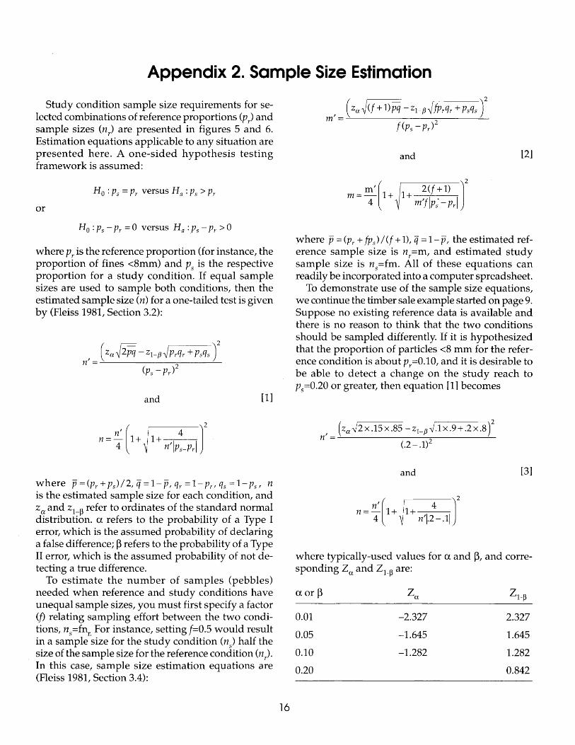
Appendix 2. Sample Size Estimation

Study condition sample size requirements for se­lected combinations of reference proportions (pr) and sample sizes (n) are presented in figures 5 and 6. Estimation equations applicable to any situation are presented here. A one-sided hypothesis testing framework is assumed:

H 0 : p 5 = p r versus H a : p 5 > p r

or

H 0 : Ps- Pr = 0 versus Ha :p5 - Pr > 0

where Pr is the reference proportion (for instance, the proportion of fines <8mm) and Psis the respective proportion for a study condition. If equal sample sizes are used to sample both conditions, then the estimated sample size (n) for a one-tailed test is given by (Fleiss 1981, Section 3.2):

n' = ( za.[2.'Pq- zi-P~p,q, + p,q, )'

(ps-Pr) 2

and

n = ~ (1 + 1 + --:--4-----:-]

2

4 n'IPs-Prl

[1]

where p=(pr +p5 )/2, q=1-p, qr =1-pr, qs =1-p5 , n is the estimated sample size for each condition, and za and z1_~ refer to ordinates of the standard normal distribution. a refers to the probability of a Type I error, which is the assumed probability of declaring a false difference;~ refers to the probability of a Type II error, which is the assumed probability of not de­tecting a true difference.

To estimate the number of samples (pebbles) needed when reference and study conditions have unequal sample sizes, you must first specify a factor (j) relating sampling effort between the two condi­tions, n

5=fnr. For instance, setting f=0.5 would result

in a sample size for the study condition (n) half the size of the sample size for the reference condition (nr). In this case, sample size estimation equations are (Fleiss 1981, Section 3.4):

16

m' = ( Za~(f + l)pq -ZJ-p~fp,q, +p,q, )'

f(ps-Pr) 2

and

m = :' (1 + 1 + 2 (/ + 1) J2 m'flp;- Prl

[2]

where p = <Pr + fp)/(f + 1), q = 1-p, the estimated ref­erence sample size is nr=m, and estimated study sample size is n

5=fm. All of these equations can

readily be incorporated into a computer spreadsheet. To demonstrate use of the sample size equations,

we continue the timber sale example started on page 9. Suppose no existing reference data is available and there is no reason to think that the two conditions should be sampled differently. If it is hypothesized that the proportion of particles <8 mm for the refer­ence condition is about Pr=0.10, and it is desirable to be able to detect a change on the study reach to p

5=0.20 or greater, then equation [1] becomes

n' = (za--J2x.15x.85 -z1_13 --).1x.9+.2x.8 t (.2- .1)2

and

n = ~ [1 + 1 + ------,---4------,- J

2

4 n'l.2- .11

[3]

where typically-used values for a and ~' and corre­sponding za and zl-~ are:

a or~

0.01

0.05

0.10

0.20

-2.327

-1.645

-1.282

2.327

1.645

1.282

0.842

Table A2 contains sample size estimates from equa­tion [3] for these levels of Type I and Type II error. Tables A3 and A4 contain unequal sample size esti­mates using equation [2], and f=l/2 and f=l/3, re­spectively. In this example, standard values of a=O.OS

Table A2.-Equal sample sizes for P, = 0. 10 and Ps = 0.20.

a

~ 0.01 0.05 0.10

0.01 566 417 347

0.05 419 293 236

0.10 349 236 185

0.20 275 177 134

Table A3.-Unequal sample size estimates (f = 1/2) for P, = 0.10 and Ps = 0.20.

a

~ 0.01 0.05 0.10

0.01 n, = 848, ns = 424 n,= 635, ns = 318 n, = 534, ns = 267

0.05 n,= 617, ns = 309 n, = 439, ns = 220 n,= 357, ns = 179

0.10 n, = 510, ns = 255 n,= 350, ns = 175 n, = 278, ns = 139

0.20 n, = 394, ns = 197 n, = 257, ns = 129 n, = 197' ns = 99

-t: U.S. GOVERNMENT PRINTING OFFICE: 1995-675-196

17

and ~=0.20 were initially assumed for Type I and Type II error levels. Sample size estimates for these error levels are read from the middle cell/bottom row of tables A2-A4. For equal sampling of reference and study conditions, estimated nr=n

5=177. If reference

and study conditions are sampled unequally, then alternative sample sizes to consider are (1) nr =257 and n

5=129, or (2) nr=336 and n

5=112. If it were more ap­

propriate to assume equal risk for Type I and Type II errors, then estimated sample sizes would be read from the diagonal cells of Tab~es A2-A4. For instance, assuming a=~=O.OS, alternative sample sizes to consider are (1) nr=n

5=293, (2) nr=439 and n

5=220, or (3) nr=583

and n5=191.

~

0.01

0.05

0.10

0.20

Table A4.-Unequal sample size estimates (f = 1/3) for P, = 0.10 and Ps = 0.20.

a

0.01 0.05 0.10

n, = 1127' ns = 376 n, = 849, ns = 283 n, = 718, ns = 240

n, = 813' ns = 271 n, = 583, ns = 191 n, = 476, ns = 159

n, = 668, ns = 223 n, = 462, ns = 154 n, = 368, ns = 123

n,= 513, ns = 171 n,= 336, ns = 112 n, = 259, ns = 87

Acknowledgments

Corky Ohlander motivated us to pursue our pebble count procedure. Corky's exhaustive review and knowledge of the Clean Water Act gave us a firm foundation for "going to the stream." We also greatly appreciate the pebble-counting efforts of Mark Hight, Robert Rush, and Brent Jenkins, and the hospitality of horse packer Gary Carver. Working in remote loca­tions occupied by grizzly bears can be unnerving. Without the critical manu­script reviews offered by Pete Hawkins, Corky Ohlander, John Potyondy, Lee MacDonald, Larry Schmidt, Charles Troendle, and David Turner our document would not be past the starting gate. It is much improved be­cause of their suggestions. Donna Sullenger drew the zig-zag procedure illustration.

The United States Department of Agriculture (USDA) prohibits discrimi­nation in its programs on the basis of race, color, national origin, sex, reli­gion, age, disability, political beliefs and marital or familial status. (Not all prohibited bases apply to all programs.) Persons with disabilities who re­quire alternative means for communication of program information (braille, large print, audiotape, etc.) should contact the USDA Office of Communi­cations at (202) 720-5881 (voice) or (202) 720-7808 (TDD).

To file a complaint, write the Secretary of Agriculture, U.S. Department of Agriculture, Washington, DC 20250, or call (202) 720-7327 (voice) or (202) 720-1127 (TDD). USDA is an equal employment opportunity employer.

Rocky Mountains

Southwest

Great Plains

U.S. Department of Agriculture Forest Service

Rocky Mountain Forest and Range Experiment Station

The Rocky Mountain Station is one of eight regional experiment stations, plus the Forest Products Laboratory and the Washington Office Staff, that make up the Forest Service research organization.

RESEARCH FOCUS

Research programs at the Rocky Mountain Station are coordinated with area universities and with other institutions. Many studies are conducted on a cooperative basis to accelerate solutions to problems involving range, water, wildlife and fish habitat, human and community development, timber, recreation, protection, and multiresource evaluation.

RESEARCH LOCATIONS

Research Work Units of the Rocky Mountain Station are operated in cooperation with universities in the following cities:

Albuquerque, New Mexico Flagstaff, Arizona Fort Collins, Colorado· Laramie, Wyoming Lincoln, Nebraska Rapid City, South Dakota

*Station Headquarters: 240 W. Prospect Rd., Fort Collins, CO 80526