A PARTICLE SIZE DISTRIBUTION FUNCTION FOR DATA …

Ann. Occup, Hyg. Vol. 11, pp. 87-98. Pergamon Press 1968. Printed in Great Britain

A PARTICLE SIZE DISTRIBUTION FUNCTION FORDATA RECORDED IN SIZE RANGES

G. A. SEHMEL

Battelle Memorial Institute, Pacific Northwest Laboratory, Richland, Washington; U.S.A.

(Received S June 1967; in revised/arm 2S September 1967)

Abstract-A method was developed for obtaining a mathematical function for the probabilitydensity of particle size when the measured distributions are in terms of size increments. Themethod is particularly applicable when a measured size distribution does not correspond tothe normal, log-normal or Weibull distributions but it can also be applied to these distributions over the limits of the experimental data. An iterative least squares technique is used tofit a partial probability density function over the size range of the experimental data. Particle'size data are represented which were initially grouped into seven size increments, but themethod is applicable to any number of size increments.

INTRODUCTION

SEVERAL distribution functions have been used to represent particle size. Theyinclude .the log-normal (GREEN and LANE, 1964), mixed exponential (GREEN andLANE, 1964; MUGELLE and EVANS, 1951), Mugelle-Evans upper-limit function(GREEN and LANE, 1964; MUGELLE and EVANS, 1951), normal (GREEN and LANE,

1964; MUGELLE and, EVANS, 1951), Nukiyama-Tanasawa (GREEN and LANE, 1964;MUGELLE and EVANS, 1951), Rosin Ramler (GREEN and LANE, 1964; MUGELLE andEVANS, 1951) and Weibull (KAO, 1959). The value of these distributions has been thatif data were well represented by a particular one, this function was an economicalmethod of summarizing the data. This summarization, especially by ·the normaldistributions, has been a convenient method of comparing experimental data forparticle size distributions. Also, some relationships have been developed betweenparameters, such as the arithmetic mean diameter and the volume mean diameter.

The distribution functions are all empirical, except for the log-normal, whichmay sometimes be justified on the basis of processes associated with origin of theparticles. Although the log-normal distribution is often used to fit data, one may' beequally justified in choosing another probability density function as long as the dataare fitted accurately. Other distribution functions would include any empiricalrelationship. For these relationships, the principal theoretical problem is that thelimit of particle size may not be infinity; the integral over particle size of the calculated probabilitydensity function will not then be equal to unity.

In many studies of particle transport we are interested in determining the behaviourof each particle size. For example, inertial impaction (SEHMEL, 1967) of particles ona surface is proportional to the squa~e of the particle size, the deposition of particles

87

at Pennsylvania State University on M

arch 4, 2016http://annhyg.oxfordjournals.org/

Dow

nloaded from

http://annhyg.oxfordjournals.org/

88 G. A. SEHMEL

(SEHMEL, 1966; 1967) from a turbulent air stream upon the surfaces of a conduitmay be proportional to a power of the particle size exceeding the fourth, and errors(SEHMEL, 1967) associated with the sampling of aerosols from an air stream are afunction of particle size. In these cases the integration limits for the probabilitydensity function are of no practical significance since we wish to determine thebehaviour of each particle size. An accurate, even though empirical representationof the particle size distribution, is often required from the grouped data of particlediameter.

Particle behaviour can most readily be studied by using nearly uniform aerosols.If the physical properties of the materials which can be dispersed in this way do notmeet experimental criteria, an aerosol of non-uniform size must be used. In thiscase, the correct number of each size particle may have to be determined from anaerosol containing many particle sizes. In some experiments, even When a nearlyuniform aerosol can be used, contamination of the equipment with particles ofseveral sizes may ultimately require the use of particle sizing and size distributionanalysis.

Much work has been done on the development of automatic devices and instrumental aids to increase the accuracy and the rapidity with which particle size analysescan be made. In general, the output from each method is the same as that obtainedthrough the use of a calibrated graticule in the eyepiece of a microscope. Particlesare sized and each is recorded as having a diameter within one of a series of sizeincrements. The data must then be processed by some method of interpolation todetermine the number of particles of any required size. These methods of interpolation are often based upon representing the data by normaL log-normal, orWeibull distributions. In a recent study (SEHMEL, 1967) these three methods werefound inadequate so that a new systematic method of representing the size distribution data was required.

The purpose of the present paper is to present the method developed for fittinggrouped particle size data in which no functional relationship describing the probability density function can be postulated a priori. The method is applicable to anyparticle size analysis. The applicability of the method to both experimental data andassumed classical distributions will be shown.

NOMENCLATURE

Ct,« Calculated percentage of particles for iteration n, within an interval AXi.

E, Experimental percentage within an interval Isx],

f Probability density function.F Cumulative distribution function.i Subscript for particles within an interval.

N Total number of particles in an experimental distribution.Q Sum of squares, see equation (6).

x, Xi Random variable which is particle diameter size.Xi Midpoint size of an increment.Yi Number percent of particles experimentally determined of size within the increment, Axi.Yi See equation (5).

Sx, Increment width.e: Differential increase.[L Mean size in normal distribution.o Variance.



Dow

nloaded from


A particle size distribution function for data recorded in size ranges 89

GRAPHICAL REPRESENTATION OF SIZE DISTRIBUTION DATA

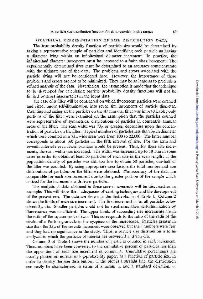
The true probability density function of particle size would be determined bytaking a representative sample of particles and identifying each particle as havinga diameter lying within an infinitesimal diameter increment. In practice, theinfinitesimal diameter increments must be increased to a finite class increment. Theexperimentally determined sizes must be determined to an accuracy commensuratewith the ultimate use of the data. The problems and errors associated with theparticle sizing will not be considered here. However, the importance of theseproblems and errors are not to be minimized. They may be so large as to preclude arefined analysis of the data. Nevertheless, the assumption is made that the techniqueto be developed for calculating particle probability density functions will not belimited by gross inaccuracies in the input data.

The case of a filter will be considered on which fluorescent particles were countedand sized, under self-illumination, into seven size increments of particle diameter.Counting and sizing all the particles on the 47 mm dia. filter was impracticable; onlyportions of the filter were examined on the assumption that the particles countedwere representative of symmetrical distributions of particles in concentric annularareas of the filter. The scan width was 73(1. or greater, depending upon the concentration of particles on the filter. Typical numbers of particles less than 3(1. in diameterwhich were counted in a 73(1. wide scan were from ·800 to 22,000. The latter numbercorresponds to about 160 particles in the fifth interval of size. For the sixth andseventh intervals even fewer particles would be present. Thus, for these size increments, the scan width was increased. The width was increased up to 10 mm in somecases in order to obtain at least 50 particles of each size in the scan length; if thepopulation density of particles was still too low to obtain 50 particles, one-half ofthe filter was counted. By using appropriate area factors the total number and sizedistribution of particles on the filter were obtained. The accuracy of the data arecomparable for each size increment due to the greater portion of the sample whichis sized for the increments with fewer particles.

The analysis of data obtained in these seven increments will be discussed as anexample. This will show the inadequacies of existing techniques and the developmentof the present one. The data are shown in the first column of Table 1. Column 2shows the limits of each size increment. The first increment is for all particles belowabout 3(1. dia. Smaller particles could not be sized since their self-illumination byfluorescence was insufficient. The upper limits of succeeding size increments are inthe ratio of the square root of two. This corresponds to the ratio of the radii of thecircles of a Porton graticule in the eyepiece of the microscope. Particles greater insize than the 25(1. of the seventh increment were observed but their numbers were fewand they had no significance in the study. Thus, a particle size distribution is to beanalyzed in which the particles of interest are between 3 and 25(1. dia.

Column 3 of Table 1 shows the number of particles counted in each increment.These numbers have been converted to the cumulative percent of particles less thanthe upper limit of each size increment in column 4. Cumulative percentages areusually plotted on normal or log-probability paper, as a function of particle size, inorder to display the size distribution; if the plot is a straight line, the distributioncan easily be characterized in terms of a mean, (1., and a standard deviation, cr.



Dow

nloaded from


90 G. A. SEHMEL

TABLE 1. CALCULATION OF CUMULATIVE SIZE DISTRIB,UTION

Diameter* ofCumulative %

Number of less thansize increment particles-in upper limit of

Increment (microns) size increment size incrementnumber XL to XH Yi F

1 0 3·14 3200 72·22 3·14 4·45 533 84·23 4·45 6·28 201 88·74 6·28 8·90 94 90·95 8·90 12·56 90 92·96 12·56 17·8 193 97'97 17·8 25·2 124 100·0

TOTAL 4435

*Diameters of succeeding increments increase by the factor of V2.

50

However, if a straight line relationship is not indicated, a force-fit of a ~ and a to thedata may be misleading. Such was the situation for the data in Table 1.

The cumulative percentages are shown plotted on log-probability coordinates inFig. 1. Two facts can be seen immediately. Firstly, the data do not show a linear

99.9 ,..-- --,

Extrapolation Needed ,.

........../99 f- "98 I

95 ~SlopefatXiS90 f- FXH-Fx- E

-2EWhere F isEvaluated at

I IE' 0.5microns

5 10

Particle Diameter, microns

FIG. 1. Graphical representation of cumulative size distribution.

relationship. Secondly, the data point for the largest particle size is located at 17·8 ~.

This means that some method of extrapolation to 25~ is needed to represent thedata obtained in the seventh size increment. The extrapolation will be consideredlater. For the moment, the determination of the percentages of particles within !!J.of each whole micron of size will be considered. These percentages, lx, can be determined from Fig. I by evaluating the slopes of the cumulative distribution curve:

FX +o. - FX - o. (1)Ix=-----

20.

where € = 0·5 !J.. The limit of the equation for Ix as € approaches zero is the probability density function.j, at the particle diameter, x. The probability density function,f, has the property that the percentage of particles having diameters between x andx + dx can be written

dF =/(x)dx

with the normalizing condition

f.f(X)dX = 100.

(2)

(3)



Dow

nloaded from



The probability density function, f, calculated from the curve in Fig. 1 is shown inFig. 2. The probability density function extends from 3·6 !.I. to 17·3 !.I. and suggeststhat f is an exponential cubic function of particle size.

10 14 18 22

Particle Diameter. microns

FIG. 2. Calculated probability density function between 3 and 17fL.

The probability density function can be approximated by first assumingfto be alinear function of x. The linearity is ascertained by finding the ratios of the experimental percentage of particles, Ei' to the lengths of the size increments, ~Xi, andplotting the ratio against the average particle size in each increment. The object is toobtain an easily determined first approximation to f The calculations are shown inTable 2. The size increments are shown in column 2 and are seen to increase with

TABLE 2. CALCULATION OF INITIAL APPROXIMATION OF THE PROBABILITY DENSITY FUNCTION

Incrementnumber

1234567

Size increment6x = (XH-XL)

(micron)

(3'14)1'311·832·623·665·247·4

Incremental %of particles of

sizes within 6xs,

(72'2)12·04·52·22·04·32·8

Ei

9·162·460·8390·5460·8210·389

Average diameterfor increment

x

3·805·377·59

10·7315·1821·5

increment number from 1·3 to 7·4 !.I.. The first increment is meaningless for approximating slopes for sizes below 3!.1. since the smallest size particle present is unknown.The linear slopes and increment midpoints shown in columns 4 and 5 are plotted onFig. 3. Included in this figure is the probability density function, f, from Fig. 2. The

10

\<::

1 t- \'-. x-'u .:»: ",c- \X

\x- I

\<l \w- 0.1 -

I\\\\\\\

0.01 I I I 1 I 1 \2 6 10 14 18 22 26

Average Particle Diameter, X. in Increment, microns

FIG. 3. Comparison of the initial estimate and the calculated probability density function.D



Dow

nloaded from


92 G. A. SEHMEL

points are seen to be located along the curve, f. By analogy, this means that thesymbol for f at the midpoint, 21·5[J., of the seventh increment should approximatethe probability density function extending from 17·8 to 25·2!J.. It will be determinedthat the probability density function can be represented by the broken line.

To summarize, an experimental size distribution has been cited which does notfollow the standard expressions used to characterize particles. The probabilitydensity function, f, approximates to an exponential cubic function of particle sizeand the true f can be approximated by first assumingf is a linear function of x withineach size increment. An analytical expression will now be derived so that the percentage in each micron particle size range can be obtained.

DEVELOPMENT OF METHOD

The present method of calculating an analytical expression for the probabilitydensity function was based on the observation that f could be initially approximatedby assuming it to be a linear function for each increment of particle size. The secondassumption is that the true probability density function is continuous. The probabilitydensity function can thus be represented by a simple expression which contains acubic in the examples cited:

f(x) = exp(a + bx + cx2 + dx"). (4)

The random variable, x, is particle size and the parameters are a, b, c, and d. For thecase under consideration there are seven observations and four parameters so thereare three degrees of freedom.

The following terminology is used: The number of particles in each size incrementis Yi, the total number of particles counted is N, ti.xi are the incremental intervals,and Xi are the midpoints of the intervals. The Xi are held constant and an iterativetechnique is used to determine the quantity;

Yi = In[fi], (5)

wherefi is the probability density function at Xi. A least squares technique is used tominimize the quantity,

n

Q = 2: [y, - (a + ss, + eXi' + dX,')J2,

i=2

(6)

(7)

with respect to the parameters in the probability density function; this determinesthe constants, a, b, c, and d.

The values of fi are initially determined by assuming the linearity

-r. 100 YiJi,l = N ti.Xi •

Having now obtained the parameters from an initial least squares fit, the probabilitydensity function

(8)



Dow

nloaded from



(9)

can be integrated between the limits of each class interval. Thus, the calculatedfraction, Ci,h in any interval is calculated from the first estimation of the probabilitydensity function by the equation

fX H

Cu. = hdxXL

in which the limits of integration are the size limits of each size increment. Values ofCu. can be calculated for class increments two through seven, but are meaninglessfor increment one.

For the second trial to determine the true probability density function, the valuesof the initial approximations of the probability density function are adjusted tominimize the difference between the calculated, Ci,l, and the experimental, Ei,percentage of particles in each size increment. The adjustments are

Ei- c.;ii,2 = ii,l+ ~ (10)

Xi

where the subscript 1 refers to the first estimate and 2 refers to the second estimate ofii. For the second trial, equation (5) for Yi is

Yi = In[!i,2] (II)

and the procedure repeated of calculating a least squares curve for the probabilitydensity function, integrating the probability density function; and comparing thecalculated and experimental percentages in each increment to determine new inputdata for the least squares fit:

e. - cc.: ( )!i,n = fi,n-l + ~ . 12

Xi

The parameters in the probability density function were found to converge by thefifth iteration. This procedure has been applied to experimental data and to assumedstandard distributions.

FITTING EXPERIMENTAL DATA

The method outlined above was used to process the data in Table 1. The solidand dashed curve shown in Fig. 3 was determined in this manner; from it thepercentages of particles having diameters between 3IL and 25IL can be found.However, the cumulative distribution function may be desirable. In this case theprobability density function can be integrated beyond the size limits used todetermine the analytical expression. This was done in the present situation forparticle sizes between 25IL and 50IL. This permits the graphing of a point at 25IL,but does not suggest that this point can be used to predict the percentage of particlesabove 25 IL.

The method was applied to obtain experimental distribution functions for typicalcurves shown as A, B, and C, in Fig. 4. Curve B is the example curve discussed.These three curves show wide ranges of size distribution and all are fitted by thetechnique. The probability density functions for these curves are shown in Fig. 5.The first estimates are good approximations to the probability density functions; avariety of forms may be fitted. The technique has now been shown to represent three



Dow

nloaded from


94 G. A. SEHMEL

99.9999

99.999

99.99

- 99.9

~c; 99

Vi

~ 90

c:

c,

50Z~

10

10 50


FIG. 4. Typical experimental and calculated size distributions.

10

~~0-

x-<l 0.1wj-

0.01

10

!0-

x-<l 0.1...,j-

0.01

6 10 14 18 22 26

Diameter, x

6 10 14 18 22 26

Diameter, x

10 .----------,

~~0- 0.1

x<l;z- 0.01

0.001

2 6 10 14 18 22 26

Diameter, x

o Fir t E r at ; Percent in Intervals s rrn e Interval Width

_ Final Estimate ofParticle ProbabilityDensity Function, f

Xis the Average Particle Diameter in Increment, microns

FIG. 5. Typical probability density functions for experimental data.

non-standard distributions, but one may want to know how good it is for predictinga standard distribution. The fitting of several standard distributions will now beconsidered.

FITTING STANDARD FORMS

Size distributions which are normally distributed, log-normally distributed, andWeibull distributed have been fitted. These expressions each have only two parameters as compared to the four parameters of the cubic expression used for theprobability density function. The two parameters used for the normal and



Dow

nloaded from


A particle size distribution function for data recorded in size ranges 9S

log-normal distributions are the mean, fl., and the variance, 0", For the Weibull distribution the cumulative distribution function, F, is given by

F = 1 - exp[-(x - fl.)afb] (13)

in which a and b are the two parameters. The probability density function for theWeibull distribution is

f = (a/b) (x - fl.)a-l exp[- (x - fl.)a/b]

and for the normal distribution is

(14)

(15)

Size Distributionis a Straight Lineon Logarithmic

Probability Paper

6 10 14 18 22 26

2 6 10 14 18 22 26

Diameter, x

Size Distributionis a Straight line

on ArithmeticProbabi lily Paper

Diameter, x. . Percent in Interval

o FirstEstimate = Interval Width

10 r--------...,

1 -

- Final Estimate ofParticle ProbabilityDensity Function. f

10

0.01

x-<l 0.1

x- 0.1<lu..i-

Size Distributionis a Straight Line

on WeibullProbabi Iity Paper

1 1-2 6 10 14 18 22 26 0-

10

0.001

0.0001

Diameter, x

C10<I>

~Q>0-

x-<l~-

OJ2 6 10 14 18 22 26

Diameter, x

1 0.10-

x-<I 0.01u.:.-

For the log-normal distribution the variable x in the normal distribution is replacedby the logarithm of the variable x.

The following procedure was used to test the fitting of three standard distributions.Straight lines were drawn on graph paper representing normal, log-normal andWeibull distributions and the percentage indicated within each size class was determined. These fractions were used as the raw data for calculating the probabilitydensity function from the cubic expression of equation (4). The initial approximations, the ratio of percentage divided by increment width, for the probability densityfunctions are shown as circles in Fig. 6. Also shown in the lower left hand corner is a

100 r---------,

Xis the Average Particle Diameter in Increment, microns

FIG. 6. Probability density functions for assumed standard distributions.



Dow

nloaded from


96 G. A. SEHMEL

graph with a line for which the probability density function was originally assumedto be straight in order to calculate the raw data. The curves obtained after the fifthiteration of the method are shown for each of the four areas. These curves wereintegrated over particle sizes from 3[1. to 50[1.. No particles greater than 50[1. wereassumed to be present. The results of these integrations after summations are thecumulative distribution functions shown in Fig. 7. The calculated percentage from25[1. to 50[1. is included in both the calculated curve and as an eighth increment ofdata in order to plot the data point at 25[1..

99.9999 INITIAL ASSUMED DISTR IBUTION DATA

99.999 ARE STRAIGHT LINES ON

~Ll.. 99.99

~i99.9 x logarithmic Probabi lity Paper

99 • Weibull Probability Paperc: l'tIQ.> E ... Arith meticProbabi Iity Paper:=Vl 90Q.>

~~ • As Probability Density Function~~ 50 on Semi-log PaperE·-::lVlZ

6 10 14 18 22 26


99.9999 99.999999.999 Weibull j99.99 99.999 Probability .-

ELl.."0

Paper99.9 .:!:!Ll..t;; ~~ ~ ~. 99.99...... = 99 ...... =c: l'tI c: l'tI

99.9Q.> E Q.> E:=Vl 90 :=VlQ.>"O Q.>"O

~~ ~~ 99~ .!§ 50 ~ .!§::l Vl ::lVl 90z z

105010

42 5 105 10 50 50

Particle Diameter, Particle Diameter,

microns microns

FIG. 7. Calculated size distributions for assumed standard distributions.

The calculated cumulative functions are seen to fit the experimental points.However, the calculated curves are not the same stright lines from which the rawdata were obtained. This non-linearity can be seen on the graphs with log-normaland Weibull coordinates. The original straight line distributions are represented bythe broken line extension of the straight line portions of the solid curves. This deviation of the solid curve from the broken straight line is caused by the extrapolationand integration of the probability density function beyond the limits for which theconstants were determined. The calculated results are valid even though straightlines are not obtained. The precision of fit of the probability density functions forthese four standard distributions can be shown by the deviation of the calculated



Dow

nloaded from



from the experimental percentage of particles in each increment. The largest deviation shown in Table 3 is only 6 per cent-an acceptable value in any case of real datadue to the experimental problems and errors associated with sizing particles.

TABLE 3. PRECISION IN FITTING STANDARD DISTRIBUTIONS

Deviation of calculated from experimental data for assumed* straight line distribution,

100 (Gi -Ei)

Ei

Increment f Normal Log-probability Weibull

234567

0·97-0·64-0·44

1·40-0·83-0·43

0·260'611·87

-2,080·75

-0·57

4'06-3,97-1,58

5·54-2,79-0·50

0'34-1,26

6'35-5,65

2·18-1,06

*Data determined graphically.

SUMMARY

A method is presented for calculating particle size probability density functionsfrom grouped data; it is an objective analysis and minimizes investigator bias. Themethod can be used when the data can not be represented by a recognized functionalform, or when numerous size distribution analyses are required. An exponentialcubic expression for the probability density function has been shown to fit experimental, normal, log-normal, and Weibull described data. If the observations yieldmore than seven size groups, the number of constants in the probability densityfunction might be increased to improve the fit. The principal limitations are that thetrue probability density function is continuous without large fluctuations for smallsize increments, and the calculated probability density function is representative onlywithin the range of sizes for which it was established.

Over 80 size distributions have been predicted within a few percent and the methodcan be used to calculate any of the commonly calculated characteristics of a sizedistribution.

The procedure is to make a first estimate of the size probability density function,integrate it to determine the calculated number of particles in any size range, comparethe calculated with the experimentally determined number of particles and then tocontinue to adjust constants until better estimates for the probability density function,as determined by least squares, converges. Computer processing facilitates thecalculations.

It was found that the logarithm of the quotient of the percentages of particles inany size increment divided by the width of the size increment in microns, was nearlylinear with the particle size at the midpoint of the increment or, at most, could berepresented by a cubic expression on semi-log paper; the latter approximates thetrue probability density functions.

Acknowledgement-The work was supported by the United States Atomic Energy Commission.



Dow

nloaded from


98 G. A. SEHMEL

REFERENCES

GREENE, H. L. and LANE, W. R. (1964) Particulate Clouds: Dusts, Smokes and Mists pp. 229-232.D. Van Nostrand Inc., Princeton, New Jersey.

IRANI, R. 1. (1959) The interpretation of abnormalities in the log-normal distribution of particle size,J. phys. Chem., 63, 1603-1607.

MUGELLE, R. M. and EVANS, H. P. (1951) Droplet size distribution in sprays, Ind. Engng. Chern.analyt, Edn 43, 1317-1324.

KAo, J. M. K. (1959) A graphical estimation of mixed Weibull parameters in life testing of electrontubes, Technometrics 1,389-407.

SEHMEL, G. A. (1966), Particle deposition and re-entrainment in long vertical conduits, PacificNorthwest Laboratory Annual Report for 1965 in the Physical Sciences, BNWL-235-3, p.61.

SEHMEL, G. A. (1967) Errors in the subisokineticsampling of an air stream, Ann. occup. Hyg. 10,73-82.

SEHMEL, G. A. (1967) Validity of Air Samples as Affected by Anisokinetic Sampling and Depositionwithin the Sampling Line Pacific Northwest Laboratory, BNWL·,sA-1045.



Dow

nloaded from


Documents

A PARTICLE SIZE DISTRIBUTION FUNCTION FOR DATA …