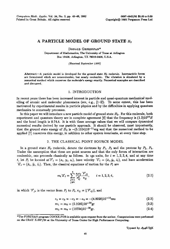
Computers Math. Applic. Vol. 24, No. 3, pp. 45-48, 1992 0097-4943/92 $5.00 + 0.00 Printed in Great Britain. All rights reserved Copyright© 1992 Pergamon Press Ltd

A PARTICLE M O D E L OF G R O U N D STATE H~

DONALD GREENSPAN*

Department of Mathematics, The University of Texas at Arlington

Box 19408, Arlington, TX 76019-0408, U.S.A.

(Received SeptemIJer 1990)

A b s t r a c t - - A particle model is developed for the ground state Ha molecule. Interparticle forces are formulated which are noncoulombic, but nearly coulomhic. The vibration is ~nu la~d by a numerical method which conserves the molecule's energy exactly. Numerical examples are described and discussed.

1. I N T R O D U C T I O N

In recent years there has been increased interest in particle and quasi-quantum mechanical modo eUing of atomic and molecular phenomena (see, e.g., [1-5]). To some extent, this has been motivated by experimental results in particle physics and by the difficulties in applying quantum mechanics to nonsteady processes.

In this paper we will introduce a new particle model of ground state//2. For this molecule, both experiment and quantum theory are in complete agreement [6] that the frequency is (1.3)1014H and the bond length is 0.74A. It is with these average values that we will compare dynamical numerical results derived by our particle approach. It should be observed, most importantly, that the ground state energy of H2 is -(5.1104)10-11erg and that the numerical method to be applied [7] conserves this energy, in addition to other system invariants, at every time step.

2. THE CLASSICAL P O I N T SOURCE MODEL

In a ground state H2 molecule, denote the electrons by P1, P3 and the protons by P2, P4. Under the assumption that these are point sources and that the only forces of interaction are coulomb/c, one proceeds classically as follows. In cgs units, for i = 1,2,3,4, and at any time t, let P~ be located at%-*/ = (x/, Yi, zi), have velocity 7 i = (z/,i]i, zi), and have acceleration "5~i = (~/, ~}i, zi). Then, the classical equations of motion for the Pi are

4 eiej "f'ji ~l l i "-~ i L.~ r?. j = l s3 rij

j#/

i - - 1,2,3,4, (2.1)

7 in which 7 j i is the vector from Pj to Pi, rij -- 11 ij]l, and

e l - e3 = - e 2 = - e 4 = - ( 4 . 8 0 2 8 ) l O - l ° e s u

m l = m 3 = ( 9 . 1 0 8 5 ) l O - 2 S g r

m 2 - - m 4 ---- ( 1 6 7 2 4 ) 1 0 - ~ S g r .

(2.2) (2.3) (2.4)

*The FORTRAN program CONXX.FOR is available upon request from the author. Computations were performed on the CRAY X-MP/24 at the University of Texas Center for High Performance Computing.

Typeset by .AA4~TEX

45

46 D. GREENSPAN

-=+ For theoretical and later computational convenience, set R = (X, Y, Z) and make the trans-

formations

_~, - - 1012"~ i (2 .5 )

T = 1022t. (2.6)

and observe that "F'~ = 101°~;~i, "~i =

1032"~. Then, dynamical equations (2.1) can be shown readily to be equivalent to

d2-RidT u -(2.5324576)'=zE (R'~j R~, / , i = 1,3

j¢i

a R, _(1.379269110_3y , d,T2 , i = 2,4 j = l

(2.7a)

(2.7b)

in which 1, if i + j is even. (2.8)

~ # - -1 , i f i + j i s o d d .

Note that from the point of view of dynamical equations (2.7a), (2.7b), one can consider the mass of any electron or proton to be unity, the charge of any electron to be - 1 and the charge of any proton to be +1, with the actual charges and masses having been incorporated into the constant 2.5324576 for each electron and into the constant (1.379269)10 -s for each proton.

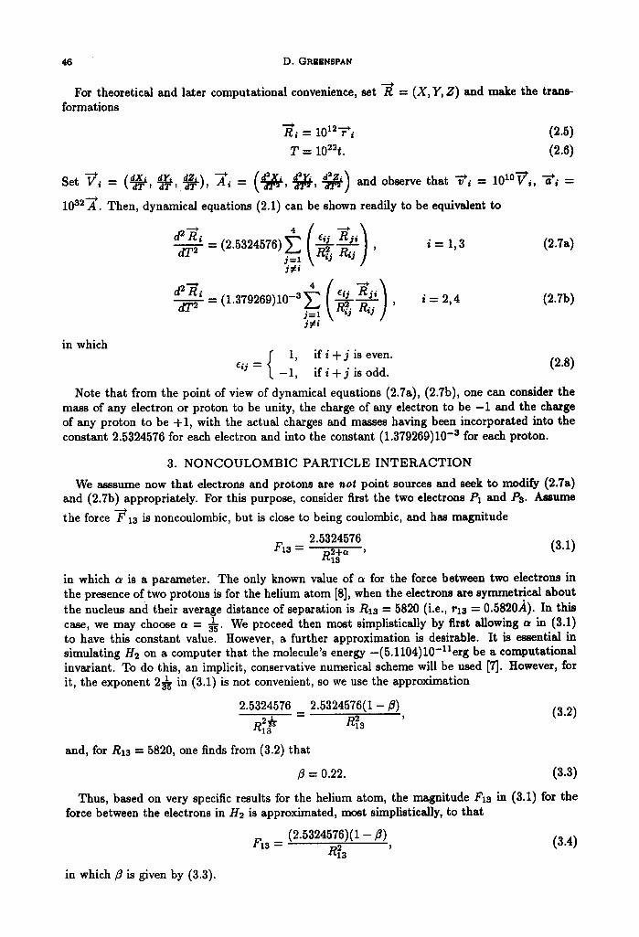
3. NONCOULOMBIC PARTICLE INTERACTION

We asssume now that electrons and protons are no~ point sources and seek to modify (2.7a) and (2.7b) appropriately. For this purpose, consider first the two electrons P1 and Ps. Assume

the force F*lS is noncoulombic, but is close to being coulombic, and has magnitude

F13 - 2.5324576 (3.1) D2+~ ' ~13

in which c~ is a parameter. The only known value of a for the force between two electrons in the presence of two protons is for the helium atom [8], when the electrons are symmetrical about the nucleus and their average distance of separation is Rza = 5820 (i.e., rza = 0.5820A). In this case, we may choose a = ~ . We proceed then most simplistically by first allowing a in (3.1) to have this constant value. However, a further approximation is desirable. It is essential in simulating H2 on a computer that the molecule's energy -(5.1104)10-Zterg be a computational invariant. To do this, an implicit, conservative numerical scheme will be used [7]. However, for it, the exponent 2~-~s in (3.1) is not convenient, so we use the approximation

2.5324576 2.5324576(1 - /~) = (3.2)

and, for Rzs = 5820, one finds from (3.2) that

/3 = 0.22. (3.3)

Thus, based on very specific results for the helium atom, the magnitude Fin in (3.1) for the force between the electrons in H2 is approximated, most simplistically, to that

F13 = (2.5324576)(1 - /~) (3.4)

in which/~ is given by (3.3).

Particle model of ground state/-/~

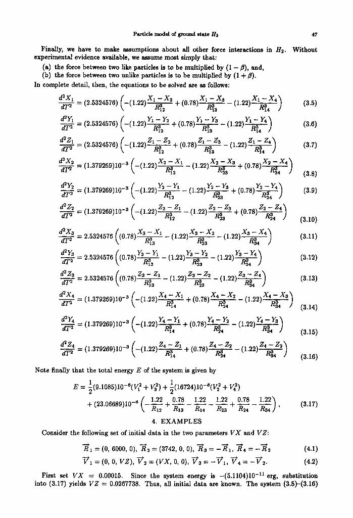
Finally, we have to make assumptions about all other force interactions in //2. experimental evidence available, we assume most simply that:

(a) the force between two like particles is to be multiplied by (1 -/~), and, (b) the force between two unlike particles is to be multiplied by (1 + 8).

In complete detail, then, the equations to be solved are as follows:

d2XldT 2 - (2.5324576) (-(1.22)X~.~X2 ÷ (O.78)X~-R~Xa (1 .22)X~ X 4 )

d2yldT2 ( ~ __Y1- Y3 YI- Y'~'~'~14 "/ = (2.5324576) -(1.22) + (0.78)----R-~ s - (1.22)

d~Z'=(2.5324576)dT 2 ( - ( 1 . 22 )Z~Z2 ÷ (0.78)ZR~Zs ( 1 . 2 2 ) Z ~ Z , )

d2X2=(1.379269)lO-adT ~ ( - ( 1 . 2 2 ) ~ a X1 (1.22)XR~Xa ÷ (0.78) X ~ X4 )

d~Y2 dT 2

d2Z~ dT 2

- - = (1.379269)10-3 (-(1.22) Y ~ Y1

= (1.379269)10 -3 (-(1.22)ZR-~laZ1

d2X----2a-2"5324576d~ ((0.78)XR~X1 ( 1 . 2 2 ) X ~ Xu ( 1 . 2 2 ) ~ )

d2Y3

d2Z3 2.5324576 ((0.78)ZR-~Z' Z s - Z2 - = _ . _ (1"22) ~ 3 (1.22) Za'R~--:4 ) dT:

d'X4 = (1 . 379269 )10 -adT 2 (-(1.22)X~'~X1 + (0.78) XR~X, (1.22) X ~ X a )

d2Y4 = (1.379269)lO_3 (_(1.22) Y4 - Y1 Y4 - Y~ ~ ) dT2 /~14 ~- (0.78) R~ 4 (1.22)

dT 2 = (1.379269)10_ s _(1.22)Z4 ~a.Z1 + (0.78)Z4 - Zu (1.22)Za - Z2~

47

Without

(3.5)

(3.6)

(3.7)

(3.8)

(3.9)

(3.10)

(3.11)

(3.12)

(3.13)

(3.14)

(3.15)

(3.16)

Note finally that the total energy E of the system is given by

= 1(9.1085)10-8(V} + Va 2) + l(16724)10-S(V~ + V~) E

( 1 . 2 2 0.78 1 .22 1 .22 0.78 1.22~ (3.17) + (23"06689)10-s \-'R-~I~ + R,---~ R,4 R2---~ + R~---~ R34 ) '

4. EXAMPLES Consider the following set of initial data in the two parameters VX and VZ:

R, - (0, 6000, 0), R 2 - (3742, 0, 0), ~3 = -R,,"* R'4 - -'R~. (4.1)

Y l = (o, o, v z ) , V2 = ( v x , o, o), V3 = --¢1, -¢, = - V s . (4.2)

First set VX = 0.00015. Since the system energy is -(5.1104)10 -11 erg, substitution into (3.17) yields VZ = 0.0267738. Thus, all initial data are known. The system (3.5)-(3.16)

48 D. GRE~NSPAN

was then solved numerically with AT = 2.0, 1.0, and 0.5. We report only on the 0.5 case, which was the most accurate. The numerical solution was generated for 5 • 10 s time steps on a CRAY X-MP/SE14. The total computing time was 9200 seconds. At each time step, the resulting nonlinear algebraic system was solved by Newtonian iteration with tolerances 10 -s for position and 10 -11 for velocity. The computer program is available in the Appendix of Greenspan [9]. The average molecular diameter which resulted was 0.77A and the frequency of oscillation was (1.57)1014H. Recall that the average diameter is 0.74.4 and frequency is (1.3)1014H.

Though changes in VX and VZ did not alter the frequency by more than (0.1)I014H, they did alter the molecular diameter more extensively. Increasing VZ increased the average molecular diameter, while decreasing VZ decreased it. For example, for the choice VZ = 0.0002, VX =

0.0261668, the average molecular diameter was 0.84A while the frequency was (1.55)1014H. A variety of other examples were run in which PI, P2, P3, P4 were repositioned. In all three-

dimensional calculations which incorporated the symmetry intrinsic in (4.1) and (4.2), the results were entirely similar to those described above. Nonsymmetric examples required time steps AT smaller than 0.01 and invariably resulted in one electron in motion near the two protons and one electron relatively distant from the protons. Finally, note that for the choice of initial data,

~ I = (0, 3742, 0), -R2 = (3742, 0, 0), "R3 = - ' R 1 , - R 4 = - R 2

V1 = (-0.0364533, O, 0), V~ = O, Va = - V 1 , V4 = V2,

(4.3) (4.4)

the molecule disintegrates into two slowly separating H atoms. Indeed, substi tut ion of (4.3) and (4.4) into (3.17) yields a system energy of -(4.35912)10 -11 erg, which is greater than tha t of/-/2 and, indeed, is twice the energy of ground s ta te H.

5. R E M A R K

With regard to the theory developed in Section 3, it would be of great value, through exper- imentM results, to be able to improve on the formulas for the noncoulombic forces between two electrons, between two protons, and between an electron and a proton.

REFERENCES

I. H. Dehraelt, Experiments on the structure of an individual elementary particle, Science 247, page 539 (1990).

2. P. Feymnan, QED, Princeton Univ. Press, Princeton, N J, (1985). 3. D. Greenspan, Deterministic modeling and computations for the states of two-electron systems with an

explicit formula for the excited states of helium, J. Chem. Phys. 84, page 300 (1986). 4. C.L. Kirschenbaum and L. Wilets, Classical many-body model for atomic collisions incorporating Heisenberg

and Pauli principles, Phys. Rev. A 21, page 834 (1980). 5. D. Levine and R. B. Berustein, Molecular Reaction Dynamic8, Clarendon, Oxford, (1974). 6. J. Hirschfelder, C. F. Curtiss and Ft. B. Byrd, Molecular Theory o] Gaaes and Liquids, Wiley, N.Y., (1954). 7. D. Greenspan, Arithmetic Applied Mathematics, Pergamon, Oxford, (1980). 8. C. DeW. Van Siclen, Estimating atomic ls orbital radii, J. Comp. Appl. M~th. 19, page 283 (1987). 9. D. Greenspan, A particle model of ground state/-/2, Technical Report 272, Math. Dept., Univ. of Texas at

Arlington, (1990).