Embed Size (px)
Citation preview

A Parametric Study of Cathode Catalyst Layer Structural
Parameters on the Performance of a PEM Fuel Cell
N. Khajeh-Hosseini D.,1 M. J. Kermani,1,∗ D. Ghadiri Moghaddam1 and J. M. Stockie2
1Department of Mechanical Engineering, Energy Conversion Research Laboratory, Amirkabir
University of Technology (Tehran Polytechnic), Tehran, Iran 15875–44132Department of Mathematics, Simon Fraser University, Burnaby, BC, Canada, V5A 1S6
Abstract
This paper is a computational study of the cathode catalyst layer (CL) of a proton exchange membrane
fuel cell (PEMFC) and how changes in its structural parameters affect performance. The underlying
mathematical model assumes homogeneous and steady-state conditions, and consists of equations that
include the effects of oxygen diffusion, electrochemical reaction rates, and transport of protons and
electrons through the Nafion ionomer (PEM) and solid phases. Simulations are concerned with the
problem of minimizing activation overpotential for a given current density. The CL consists of four
phases: ionomer, solid substrate, catalyst particles and void spaces. The void spaces are assumed to be
fully flooded by liquid water so that oxygen within the CL can diffuse to reaction sites via two routes:
within the flooded void spaces and dissolved within the ionomer phase. The net diffusive flux of oxygen
through the cathode CL is obtained by incorporating these two diffusive fluxes via a parallel resistance
type model. The effect of six structural parameters on the CL performance is considered: platinum
and carbon mass loadings, ionomer volume fraction, the extent to which the gas diffusion layer (GDL)
extends into the CL, the GDL porosity and CL thickness. Numerical simulations demonstrate that
the cathode CL performance is most strongly affected by the ionomer volume fraction, CL thickness
and carbon mass loading. These results give useful guidelines for manufactures of PEMFC catalyst layers.
Keywords: PEM fuel cell; catalyst layer; macro-homogeneous model; numerical simula-
tions; sensitivity study
∗Corresponding Author: Assistant Professor and Head of Energy Conversion Research Laboratory, Tel.: +98 21 6454
3421; Fax: +98 21 6641 9736. E-mail address: [email protected] (M.J. Kermani).
1Manuscript Submitted to Journal of Applied Electrochemistry
Khajeh-Hosseini D., Kermani, Ghadiri Moghaddam and Stockie

1 Introduction
In a proton exchange membrane fuel cell (or PEMFC), electrical energy is generated directly through
an electrochemical reaction between oxygen and hydrogen. PEMFCs have high power density, quick
start-up times, and produce power with theoretically zero emissions. These advantages make them
one of the most serious alternatives to replace the internal combustion engines. However, even with
recent advances in materials and optimization of fuel cell processes, commercialization of PEMFCs is
still being delayed pending further improvements in performance and cost.
The key electrochemical reaction in a PEMFC occurs at the cathode catalyst layer (or CL) where
oxygen and hydrogen are combined to generate an electrical current at a rate directly proportional
to the electrochemical reaction rate. The rate of reaction is mainly dependent on CL structural
parameters related to the composition and distribution of CL materials as well as how the CL is
synthesized. A robust and reliable PEMFC performance analysis requires a thorough understanding
of CL performance through extensive parametric studies. Experimental investigations are indispensible
in this regard but they can be very time-consuming and costly, particularly if many parameters are
involved (see [11] and [12]). Furthermore, it can be quite difficult to correlate the usually sparse
experimental data to specific aspects of CL structure. Therefore, numerical simulations can be very
useful in predicting and optimizing CL performance, especially in the early stages of design.
Models for the cathode CL can be broadly classified into three different categories based on their
level of complexity: interface models, macro-homogeneous models, and agglomerate models. Each
model has its advantages and disadvantages that we next discuss briefly:
Interface models were the first applied to modelling the entire fuel cell, and they have been used
commonly since then because of their simplicity. The CL is treated as an infinitely thin layer
and no attempt is made to capture spatial variations in solution profiles. Consequently, these
models are posed in terms of averaged transport parameters and so provide only limited guidance
on microstructure and performance optimization. On the other hand, interface models are
computationally efficient and so are are very suitable for multidimensional computations and
parametric studies of the entire fuel cell. For example, Berning and Djilali [1] developed a 3D,
non-isothermal model using a CFD approach, investigating the effects on fuel cell performance
of parameters such as GDL porosity and thickness, and channel width. Lum and McGuirk [2]
performed a similar study that examined the influence of permeability and oxidant concentration
as well as geometrical parameters.
Macro-homogeneous models (also called “pseudo-homogeneous” models) were first introduced by
Tiedemann and Newman [3] and consider the CL as a layer of finite thickness, with averaged
transport coefficients describing the effect of variations in compositional parameters describing
platinum catalyst, carbon support, solid GDL matrix, and electrolyte materials. Marr and Li [4]
2Manuscript Submitted to Journal of Applied Electrochemistry
Khajeh-Hosseini D., Kermani, Ghadiri Moghaddam and Stockie

used this type of model to investigate the influence of CL composition and especially platinum
loading on CL performance. They also provided experimental evidence that the CL can be
flooded with water even at very low current densities. You and Liu [5] performed simulations
using a control volume approach to study the effect of membrane conductivity and CL porosity.
Du et al. [6] performed a more extensive parametric study based on a macrohomogeneous model
in which they assumed that oxygen diffuses to active catalyst sites solely in the gas phase, while
more recent work suggests that significant oxygen transport also occurs in dissolved phase within
the ionomer.
Agglomerate models represent the most sophisticated approach, taking into account both the com-
position and structural distribution of CL materials. Particles consisting of platinum plus car-
bon support (Pt/C) are grouped in small agglomerates that are surrounded by and bonded
together with electrolyte and GDL material. A relatively uniform distribution of intra- and
inter-agglomerate materials is vital in order to correlate agglomerate structure with perfor-
mance. Beginning with the pioneering work of Ridge et al. [7], many other agglomerate models
have been developed especially in recent years. Secanell et al. [8] used parametric studies to
determine optimal values of platinum loading, Pt/C ratio, electrolyte volume fraction and the
GDL porosity, which they also showed depend on operating conditions. Shah et al. [9] developed
a 1D transient model for the entire membrane-electrode assembly (MEA) of a PEMFC, consid-
ering effects of humidification, temperature, pore size and GDL contact angle. Wang et al. [10]
studied the effect of void fraction, inflow relative humidity, and the net water transport, and
showed that low humidity operation can benefit cell performance by reducing oxygen transport
at high current densities.
Among the three types of models, the thin interface approach is the simplest and the agglomerate
approach is the most complex. The macro-homogeneous models fall somewhere in between, and have
the advantage that they can provide reliable results at low and medium cell current densities [8].
In order that a catalyst layer model is capable of reliably predicting performance, it is essential that
it captures the complex multi-material structure of the CL. Agglomerate models seem to provide the
best fit to experimental results [13]; however, it is still unclear how the agglomerates are formed and
how they are defined within the complex random multi-material morphology of the porous CL matrix.
Taking into consideration both these uncertainties and the greater complexity of the agglomerate
model, the macro-homogeneous models stand out as a more desirable alternative to obtain detailed
information about the correlations between CL structure and performance [8].
In this paper a steady-state, macro-homogeneous CL model is used to study transport in the
cathode catalyst layer within a medium range of current densities. The governing equations are a
coupled system of ODEs that capture oxygen diffusion, electrochemical reactions, and the transport of
electrons and protons. The equations are solved using a shooting algorithm that makes use of a Runge-
3Manuscript Submitted to Journal of Applied Electrochemistry
Khajeh-Hosseini D., Kermani, Ghadiri Moghaddam and Stockie
Kutta time-stepping technique to integrate the equations to steady state. Numerical simulations are
used to study the dependence of PEMFC performance on six structural parameters: platinum and
carbon mass loading, CL thickness, ionomer volume fraction, the extent of GDL penetration into the
CL, and GDL porosity. Most other studies of CL performance have focused on a limited number
of structural parameters (e.g., [1], [13]) whereas in the present study we consider a more extensive
selection of parameters. The dependent variable is the activation overpotential and parametric studies
are used to probe the effect of the structural parameters on the overpotential; in particular, minimizing
the activation overpotential at a given cell current density is the goal of this study. The results give
guidelines that should prove useful to MEA manufacturers.
2 The Model Description
A representative picture of the catalyst layer is shown schematically in Fig. 1. Hydrogen gas from the
anode is split into electrons and protons at the anode side catalyst layer. The electrons are transferred
through an external circuit to the cathode CL, while the protons move through the ionomer membrane
to the cathode side. Oxygen is supplied on the cathode side where it diffuses in gas form through void
spaces in the GDL to the GDL/CL interface.
The present study is concerned with what occurs once the three reacting species – oxygen gas,
protons and electrons – reach the cathode CL. We assume the CL consists of four distinct regions (refer
to Fig. 1): (1) catalyst clusters, consisting of platinum and carbon support; (2) Nafion ionomer phase;
(3) solid GDL phase; and (4) void spaces. Oxygen diffuses in dissolved form through the flooded void
spaces and the ionomer membrane. Hydrogen is transported as ions through through the ionomer
phases, while electrons move only through the solid conductive phase. All three reacting species – O2,
H+ and e− – reach the reaction sites on Pt/C clusters where the electrochemical reaction
O2+ 4H+ + 4e− → 2H
2O + Heat (1)
takes place. As shown in Fig. 1, the materials lying on either side of the cathode CL (i.e. GDL and
membrane) are designed such that they penetrate partially into the layer, which allows the reacting
species ready access to reaction sites. We note that the ionomer membrane is a polymer (Nafion) whose
ability to conduct protons increases with hydration level, and so maintaining sufficient hydration levels
within the CL is essential.
3 Governing Equations
In the derivation of the equations to follow, we make a number of simplifying assumptions:
1. The problem is one–dimensional and steady.
4Manuscript Submitted to Journal of Applied Electrochemistry
Khajeh-Hosseini D., Kermani, Ghadiri Moghaddam and Stockie

Pt /C
Pt /CMembrane phase
Solid phase
Void space
e-
e-
H+
H+
O2
O2
z
lc
Figure 1: Schematic of the cathode CL for a PEM fuel cell (adapted from [14]).
2. The CL is a macro-homogeneous medium consisting of the four components depicted in Fig. 1.
3. The GDL and membrane phases penetrate a well-defined distance into the CCL.
4. Operating pressure and temperature are constant.
5. Void spaces are fully flooded by liquid water.
The governing equations are split in two groups: algebraic equations governing CL composition, and
differential equations governing transport.
3.1 Algebraic Equations Governing Composition
3.1.1 Phase compositions
We first define the following volume fractions:
• εc is the void volume fraction, or CL porosity.
• Lm,c is the volume fraction of the ionomer phase.
• Lg,c is the volume fraction of the GDL penetrating into the CL. Then the volume fraction of the
solid portion of the GDL is
Ls = Lg,c(1 − εg), (2)
5Manuscript Submitted to Journal of Applied Electrochemistry
Khajeh-Hosseini D., Kermani, Ghadiri Moghaddam and Stockie

where εg is the GDL porosity.
• LPt/C is the volume fraction of the catalyst Pt/C particles.
The following equation governs the four corresponding volumes
Vtot = Vm,c + Vc + VPt/C
+ Vs, (3)
where Vtot is the total CL volume. The volume fractions can then be written as
Lm,c =Vm,c
Vtot
, εc =Vc
Vtot
, LPt/C =VPt/C
Vtot
and Ls =Vs
Vtot
, (4)
after which
Lm,c + Lg,c(1 − εg) + LPt/C
+ εc = 1 . (5)
The quantity LPt/C
in Eq. 5 can be expressed in terms of the mass loading of catalyst particles
per unit area of the cathode. Consider the total volume of the CL, Vtot = A × lc, where A is the area
of the cathode and lc is the CL thickness. Keeping in mind that VPt/C = VPt + VC , we may write
VPt =(mass)
Pt
ρPt
and VC =(mass)
C
ρC
(6)
where ρPt
and ρC
are the density of platinum and carbon repectively. Defining the mass loading of
platinum and carbon per unit area of the cathode as
mPt
≡(mass)
Pt
Aand m
C≡
(mass)C
A, (7)
we may write
LPt/C
=m
Pt
ρPt
lc+
mC
ρClc
. (8)
We then introduce the mass fraction of platinum to that of Pt/C particles,
f ≡m
Pt
mPt
+ mC
, (9)
where f = 1 for pure platinum and f = 0 for pure carbon. We substitute this expression along with
Eqs. 8 into Eq. 5 to write the CL porosity as
εc = 1 − Lm,c − Lg,c(1 − εg) −m
Pt
lc
[1
ρPt
+1 − f
f
1
ρC
]
︸ ︷︷ ︸
=LPt/C
. (10)
This expression will be used in the next section to determine the effective oxygen diffusion coefficient.
6Manuscript Submitted to Journal of Applied Electrochemistry
Khajeh-Hosseini D., Kermani, Ghadiri Moghaddam and Stockie

Void
Membrane
Solidθ
r2
r1
θ
θ
c
s
m,c
Figure 2: A cylindrical control volume element with the Pt/C particle located at the center of the
element, surrounded by the void, solid and membrane phases.
3.1.2 Oxygen diffusion coefficient
An equivalent (effective) diffusion coefficient for the oxygen species is determined in this section. To
this end, we model the diffusion of gaseous oxygen through a cylindrical control volume element of
radius r2 surrounding a single Pt/C particle with radius 0 < r1 < r2, as shown in Fig. 2. The Pt/C
particle is located at the center of the element and is surrounded by sectors containing the ionomer,
solid and void phases.
The distribution of Pt/C clusters through the entire CL is random; hence, the homogeneity as-
sumption is a reasonable one. Furthermore, the average diffusion lengths for the oxygen species
through both the void and ionomer phases is equal to (r2 − r1). According to the division of phases
depicted in Fig. 2,
2π = θm,c + θc + θs, (11)
where θm,c, θc and θs are the contact angles corresponding to ionomer, void and solid phases respec-
tively. The corresponding volumes are
Vm,c =1
2θm,c(r
22 − r2
1) ℓ Vc =1
2θc(r
22 − r2
1) ℓ Vs =1
2θs(r
22 − r2
1) ℓ (12)
where ℓ is the out-of-plane depth of the cylindrical element. From Eq. 12, we then obtain the following
identity:Vm,c
θm,c=
Vc
θc=
Vs
θs=
1
2(r2
2 − r21) ℓ. (13)
Next, in analog with thermal resistance for heat conduction in cylinders [15], we write the diffusion
resistance R as
R ≡ln (r2/r1)
θ Deff
ℓ(14)
7Manuscript Submitted to Journal of Applied Electrochemistry
Khajeh-Hosseini D., Kermani, Ghadiri Moghaddam and Stockie

where θ is the contact angle and Deff
is an effective diffusion coefficient. Oxygen reaches Pt/C reaction
sites by diffusing through two parallel routes – the ionomer phase and void spaces (which are fully
flooded by liquid water). Using Eq. 14, we can write the diffusion resistances in the ionomer (Rm,c)
and void (Rc) regions as
Rm,c =ln (r2/r1)
θm,c Deff
O2−mℓ
and Rc =ln (r2/r1)
θc Deff
O2−wℓ, (15)
where the effective diffusion coefficients (in units of m2 s−1) are denoted by Deff
O2−min the membrane
region and Deff
O2−win the water-flooded void region. According to [16], the effective diffusion coefficients
can be expressed as
Deff
O2−m= L3/2
m,c DO2−m
and Deff
O2−w= ε3/2
c DO2−w
, (16)
where DO2−w
is a function of temperature (evaluated using Wilke-Chang equation [17], with the
numerical value given in Table 2) and DO2−m
is obtained by a curve fit to experimental data [18]
DO2−m
= 1.4276 × 10⁻¹¹ T − 4.2185 × 10⁻⁹, (17)
where the temperature T is measured in degrees Kelvin.
Using Eqs. 4, 11 and 13, the contact angle for each phase can be written in terms of species volume
fractions as
θm,c =Lm,c
Lm,c + εc + Ls2π and θc =
εc
Lm,c + εc + Ls2π , (18)
following which the diffusion resistances can be obtained from Eqs. 15 as
Rm,c =Lm,c + εc + Ls
Lm,c
ln (r2/r1)
2π Deff
O2−mℓ
and Rc =Lm,c + εc + Ls
εc
ln (r2/r1)
2π Deff
O2−Wℓ
. (19)
We note that the diffusion resistance of each species is inversely proportional to its volume fraction.
Treating the individual resistances in parallel, the equivalent total diffusion resistance Req is
1
Req=
1
Rm,c+
1
Rc(20)
where we have defined
Req =ln (r2/r1)
2πDeff
O2
ℓ. (21)
The overall effective oxygen diffusion coefficient may then be found by combining Eqs. 19 and 21,
Deff
O2
= Deff
O2−m
Lm,c
Lm,c + εc + Ls+ D
eff
O2−w
εc
Lm,c + εc + Ls, (22)
in which the terms Lm,c/(Lm,c + εc + Ls) and εc/(Lm,c + εc + Ls) are, respectively, the volume frac-
tions of the ionomer and void phases within the CL.
8Manuscript Submitted to Journal of Applied Electrochemistry
Khajeh-Hosseini D., Kermani, Ghadiri Moghaddam and Stockie

3.2 Governing Differential Equations
3.2.1 Oxygen diffusion
The transport due to diffusion of oxygen within the cathode CL is assumed to follow Fick’s law [19]
NO2
= −DO2∇C
O2, (23)
where NO2
, DO2
and CO2
are, respectively, the superficial molar flux, bulk diffusion coefficient, and
concentration of oxygen. The conservation of oxygen at steady state can be expressed as
∇ · NO2
= RO2
. (24)
The consumption rate of oxygen per unit volume is denoted by RO2
, which can be related to the
protonic current density i by
RO2
= −s
nF∇ · i, (25)
where s is the stoichiometric coefficient, n is the number of electrons participating in the reaction, and
F is the Faraday constant (96485Coulombs mol−1). According to Eq. 1, we have s = 1 and n = 4
after which Eq. 25 becomes
RO2
= −1
4F
di
dz, (26)
where ∇· i is replaced by di/dz in the present 1D study. We then combine this expression with Eqs. 23
and 24 to obtain
−Deff
O2
d2CO2
dz2= −
1
4F
di
dz, (27)
where DO2
is replaced by the effective diffusion coefficient Deff
O2
(determined in Sec. 3.1.2).
As indicated later in Eqs. 43–44, this last equation is subjected to the boundary condition i = Iδ
and dCO2/dz = 0 at z = lc at the CL/membrane interface; therefore, Eq. 27 may be integrated once
to obtaindC
O2
dz=
i − Iδ
4FDeff
O2
. (28)
3.2.2 Electrochemical reaction rate
The electrochemical reaction rate is determined by the Butler-Volmer equation [19]
di
dz= a i
0
[
exp
(αcF
RTηact
)
− exp
(
−αaF
RTηact
)]
, (29)
where i0 is the exchange current density (determined experimentally for smooth-surface reaction sites),
αc and αa are the cathodic and anodic transfer coefficients, and a is the specific area that takes into
account the roughness of the reaction sites. The quantity a may be expressed as
a ≡( area )
RS
(A × lc), (30)
9Manuscript Submitted to Journal of Applied Electrochemistry
Khajeh-Hosseini D., Kermani, Ghadiri Moghaddam and Stockie

where ( area )RS
is the true area of reaction sites. Then, defining As to be the reaction surface area
per unit mass of the platinum (in units of m2 kg−1),
As ≡( area )
RS
( mass )Pt
, (31)
and we may then write
As =a lcmPt
or a =m
Pt
lcAs . (32)
A curve fitting procedure is employed in Ref. [20] to approximate As in terms of the platinum mass
fraction f according to
As = (227.79f3 − 158.57f2 − 201.53f + 159.5) × 103 . (33)
In Eq. 29, i0
is the exchange current density which is usually expressed in terms of a reference
exchange current density i0,ref
and reference concentration CO2,ref
[21] by
i0
= i0,ref
(
CO2
CO2,ref
)γO2
, (34)
where γO2
is the reaction order for the oxygen (and we take γ = 1 as recommended by Newman and
Thoma-Alyea [22]. The ratio(
CO2
/CO2,ref
)γO2 in Eq. 34 is in fact a correction factor for the deviation
of concentration from the reference state. The reference exchange current density i0,ref
from Eq. 34 (in
Am−2) is obtained from another curve fit to the experimental data provided in Ref. [18],
i0,ref
= 10 0.03741T − 16.96 , (35)
where T is the temperature in degrees Kelvin. Refer to Table 2 for values of the parameters appearing
in the above equations.
3.2.3 Activation overpotential
The activation overpotential within the CL is caused by ohmic losses due to the protonic resistance
in the ionomer phase and electrical resistance in the solid phase, according to [4]
dηact
dz=
i
κeff
+i − I
δ
σeff
. (36)
The effective protonic conductivity κeff
can be related to its bulk value κ and the ionomer volume
fraction via [16]
κeff = (Lm,c)3/2 κ . (37)
Similarly, the effective electronic conductivity may be written as
σeff = (1 − Lm,c − εc)3/2σ . (38)
Eqs. 28, 29 and 36 comprise a coupled system of nonlinear ODE’s in the unknowns CO2
, i and ηact
that govern transport of oxygen, protons and electrons within the cathode CL.
10Manuscript Submitted to Journal of Applied Electrochemistry
Khajeh-Hosseini D., Kermani, Ghadiri Moghaddam and Stockie

4 Boundary Conditions
In order to obtain a well-posed problem, we must supplement the equations derived in the previous
section with a number of boundary conditions which we describe next.
• At the GDL/CL interface, z = 0: Oxygen enters the CL pores from the GDL, and since
the pores are assumed to be flooded with liquid water, the oxygen passes through the GDL/CL
interface at z = 0 by first dissolving in water. The oxygen concentration at the interface is
therefore determined using Henry’s Law
CO2|z=0
=P
O2
HO2
, (39)
where the oxygen partial pressure
PO2
= xO2
P, (40)
xO2
is the oxygen mole fraction, and P is the gas mixture pressure at the GDL/CL interface. The
Henry constant HO2
(in atm m3 mol−1) is typically assumed to be a function of temperature [21]
according to
HO2
= 1.33 exp
(
−666
T
)
, (41)
where T is measured in degrees Kelvin. Because the GDL is very thin, the pressure conditions
at the GDL/CL interface are set to the cathode channel values, which we take to be xO2
= 0.21
and P = 5 atm.
The boundary condition for the protonic current density comes from the assumption that all
protons are consumed before they reach the GDL/CL boundary, so that
i|z=0 = 0. (42)
• At the CL/membrane interface, z = lc: The protonic current density at the membrane
approaches its ultimate value (i.e., the cell current density, Iδ), so that
i|z=lc = Iδ. (43)
Also, oxygen cannot reach this boundary because it is totally consumed within a narrow band
in the vicinity of the GDL, so that
−dC
O2
dz
∣∣∣∣z=lc
= 0. (44)
11Manuscript Submitted to Journal of Applied Electrochemistry
Khajeh-Hosseini D., Kermani, Ghadiri Moghaddam and Stockie
5 Solution Procedure
The ODEs consisting of Eqs. 28, 29 and 36 along with boundary conditions Eqs. 39, 42–44 represent
a two-point boundary value problem. We employ a shooting method in which a guess is made for
ηact |z=0at the GDL/CL interface, and then we iterate on the solution until i → Iδ at z = lc. A
Newton-Raphson method has also been used to speed up the convergence of the iteration [23].
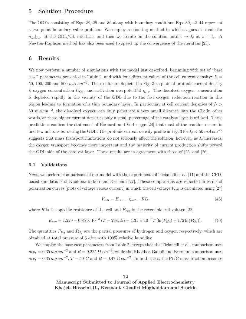
6 Results
We now perform a number of simulations with the model just described, beginning with set of “base
case” parameters presented in Table 2, and with four different values of the cell current density: Iδ =
50, 100, 200 and 500 mA cm−2. The results are depicted in Fig. 3 as plots of protonic current density
i, oxygen concentration CO2, and activation overpotential ηact . The dissolved oxygen concentration
is depleted rapidly in the vicinity of the GDL due to the fast oxygen reduction reaction in this
region leading to formation of a thin boundary layer. In particular, at cell current densities of Iδ >
50 mAcm−2, the dissolved oxygen can only penetrate a very small distance into the CL; in other
words, at these higher current densities only a small percentage of the catalyst layer is utilized. These
predictions confirm the statement of Bernardi and Verbrugge [24] that most of the reaction occurs in
first few microns bordering the GDL. The protonic current density profile in Fig. 3 for Iδ < 50 mAcm−2
suggests that mass transport limitations do not seriously affect the solution; however, as Iδ increases,
the oxygen transport becomes more important and the majority of current production shifts toward
the GDL side of the catalyst layer. These results are in agreement with those of [25] and [26].
6.1 Validations
Next, we perform comparisons of our model with the experiments of Ticianelli et al. [11] and the CFD-
based simulations of Khakbaz-Baboli and Kermani [27]. These comparisons are reported in terms of
polarization curves (plots of voltage versus current) in which the cell voltage Vcell is calculated using [27]
Vcell = Erev − ηact − RIδ, (45)
where R is the specific resistance of the cell and Erev is the reversible cell voltage [28]
Erev = 1.229 − 0.85 × 10⁻³ (T − 298.15) + 4.31 × 10⁻⁵T [ln(PH2) + 1/2 ln(PO2
)] . (46)
The quantities PH2and PO2
are the partial pressures of hydrogen and oxygen respectively, which are
obtained at total pressure of 5 atm with 100% relative humidity.
We employ the base case parameters from Table 2, except that the Ticianelli et al. comparison uses
mPt = 0.35mg cm−2 and R = 0.225 Ω cm−2, while the Khakbaz-Baboli and Kermani comparison uses
mPt = 0.35mg cm−2, T = 50oC and R = 0.47 Ω cm−2. In both cases, the Pt/C mass fraction becomes
12Manuscript Submitted to Journal of Applied Electrochemistry
Khajeh-Hosseini D., Kermani, Ghadiri Moghaddam and Stockie

f = 10 Mass% (Pt/C) using the base value of mC = 4.5mg cm−2. Fig. 4 depicts the polarization
curves and demonstrates that our computations match very well with the previously published results
in both cases. The breakdown of losses (in terms of activation and ohmic losses) is also shown in
Fig. 5, where according to Eq. 45 the sum of the losses subtracted from the reversible cell voltage
gives Vcell.
6.2 Parametric Studies
We next perform a detailed parametric study of the effect on activation potential of changes in the
following parameters: (i) platinum mass loading per unit area, mPt; (ii) carbon mass loading per
unit area, mC ; (iii) volume fraction of ionomer phase, Lm,c; (iv) volume fraction of GDL material
penetrating the CL, Lg,c; (v) GDL porosity, εg; and (vi) CL thickness lc. The parameters are grouped
in pairs and the results are summarized in the next three sections.
6.2.1 Effect of Lg,c and Lm,c
In this section, we study the effect of changes in GDL and ionomer volume fractions on cell perfor-
mance. In fact, when the MEA is synthesized there is ideally no penetration of the GDL into the
CL; however, after the cell is assembled the MEA comes under a compressive load which can cause
the GDL to penetrate into the catalyst. If the GDL is composed of a flexible carbon cloth material
such as we consider in this study, it may experience large deformations into the gas channels etched
in bipolar plates as well as significant penetration into the CL. We note that the observed degree of
GDL penetration is not very large, with Lg,c lying in the range of 5 ≤ Lg,c ≤ 15 Vol.%.
Fig. 6 shows the variation of activation overpotential with Lg,c and Lm,c for different values of
platinum mass fraction f (where we have actually varied mC to effect changes in f). The vertical
axes are chosen identical in both plots so that it is obvious that the effect of changes in GDL fraction
are much larger than for the membrane fraction. In Fig. 6-(Left), the curves increase slightly (i.e.,
performance degrades) with increases in Lg,c primarily because of the increase in CL porosity εc and
corresponding decrease in Deff
O2
. On the other hand, as f increases the activation overpotential falls
(and hence performance improves) since the specific area of the reaction sites (a) increases with f (see
Eq. 32).
From the corresponding curves for ionomer volume fraction in Fig. 6-(Right), the activation over-
potential actually decreases with increasing Lm,c. This can be explained by observing that εc (and
hence also Deff
O2
) decreases with increasing Lm,c (see Eq. 10). On the other hand, the protonic con-
ductivity κeff
increases with Lm,c according to Eq. 37, so that changes in Lm,c have two opposing
influences on CL performance with the net effect being to reduce ηact as Lm,c increases.
13Manuscript Submitted to Journal of Applied Electrochemistry
Khajeh-Hosseini D., Kermani, Ghadiri Moghaddam and Stockie

6.2.2 Effect of mPt and mC
The two plots in Fig. 7 depict the variation of activation overpotential in response to changes in
platinum mass fraction f for different values of mPt and mC . For f lying within the interval [0.1, 0.3],
variations in ηact are about the same magnitude; however, the activation overpotential is more sensitive
to mC than mPt. These simulations predict that the best CL performance occurs for the largest value
of f = 30Mass%.
We focus first on changes in mPt shown in Fig. 7-(Left), where we observe that for all values except
the largest (mPt = 0.6 mAcm−2) the activation overpotential decreases monotonically with f . Also,
the performance is less sensitive to mPt at larger f values, say when f ≥ 20Mass%. In fact, increasing
f has two competing effects on CL performance:
Effect 1: As f increases over the [0.1, 0.3], the reaction surface area As decreases according to Eq. 33,
which leads to a corresponding decrease in a (from Eq. 32). This has a negative influence on CL
performance.
Effect 2: On the other hand, when mPt is held constant as f increases, the carbon loading mC must
decrease according to the definition f = mPt/(mPt + mC); that is, the contribution of the solid
carbon particles within the CL decreases. This results in an increase in both CL porosity εc (see
Eq. 10) and hence also oxygen diffusivity Deff
O2
, which in turn improves CL performance.
These two effects therefore compete with each other with the net result being that ηact decreases with
f as shown in Fig. 7-(Left).
Next we consider the right hand plot in Fig. 7, where curves of constant mC decrease with increasing
f . Analogous to the argument used for the mPt curves above, there are two competing effects on CL
performance with the net result that increasing f improves performance. On the other hand, increasing
the carbon loading (while holding f fixed) results in a decrease in performance owing to the presence
of less platinum.
6.2.3 Effect εg and lc
The two plots in Fig. 9 depict the variation of ηact with mPt and show that CL performance increases
with mPt, which is primarily due to the fact that the specific area of reaction sites a also increases.
The left hand plot includes curves for several values of GDL porosity, from which it is clear that the
activation overpotential is relatively insensitive to changes in εg.
Fig. 9-(Right) shows the effect of changes in CL thickness on performance. In contrast with the
εg plots, we see here much more significant variation from one curve to the next. Indeed, as the
CL thickness lc (or equivalently, the carbon loading mC) is increased, there is a considerable drop in
performance owing to increased ohmic losses. The variations in mPt along each curve correspond to
14Manuscript Submitted to Journal of Applied Electrochemistry
Khajeh-Hosseini D., Kermani, Ghadiri Moghaddam and Stockie

values of f ranging between 10–50 Mass%, where points A, B and C refer to values of f = 10, 30 and
50 respectively.
It is important to note here that increasing the platinum loading is not the best way to optimize
performance. Indeed, beyond the point B identified on the mPt − ηact curves in Fig. 9-(Right) (corre-
sponding to f = 30), the slope of the curve becomes so small that further efforts to increase platinum
loading are not likely to lead to any significant improvment when considered in terms of a cost/benefit
analysis. Similar conclusions were drawn by Cho et al. [29] in an experimental study using X-ray
diffraction and cyclic voltametry measurement techniques. Instead, the best results are likely to be
obtained using a multi-parameter design optimization which combines an efforts to increase Pt mass
fraction with reductions in CL thickness.
7 Concluding Remarks
A comprehensive parametric study of CL performance was carried out by investigating the effects on
activation overpotential of variations in six structural parameters: mPt, mC , Lm,c, Lg,c, εg and lc. The
underlying mathematical model consists of a system of coupled nonlinear ODEs governing diffusion,
electrochemical reactions and ohmic losses (given by Eqs. 28, 29 and 36). These equations, subjected
to the boundary conditions given in Sec. 4, are solved using a shooting algorithm. The highlights of
the results are summarized below:
• The effect of changes in the six parameters can be interpreted more easily by using two key
intermediate parameters: namely, the specific area of the reaction sites a and CL porosity εc. In
general, increasing either a or εc leads to improvements in performance.
• The results of the parameter study are summarized in Table 1 in terms of the range, optimum
value, and sensitivity for each parameter considered. The parameters are also ranked from 1
to 6 in order of their importance, with the rank 1 for Lm,c indicating that it is the structural
parameter that has the most significant influence on CL performance. We note that the optimum
Table 1: Summary of the results for the parametric study.
Rank structural ranges optimum sensitivity
parameter studied value (∆ηact / V)
1 Lm,c /Vol.% 10 − 50 50 0.35
2 lc /µm 10 − 50 10 0.07
3 mC /mg cm−2 2 − 4 2 0.025
4 mPt /mg cm−2 0.4 − 0.6 0.4 0.015
5 Lg,c /Vol.% 5 − 15 5 0.01
6 εg /Vol.% 30 − 50 50 ≈ 0
15Manuscript Submitted to Journal of Applied Electrochemistry
Khajeh-Hosseini D., Kermani, Ghadiri Moghaddam and Stockie

performance is achieved in all cases at one of the endpoints of the range for the corresponding
parameter.
• We observe the best performance in a narrow band of mPt, and for values outside of this range
any increase in platinum loading is probably not economically justifiable. Similarly, Figs. 6 and 7
demonstrated that the best performance occurs at the highest value of platinum mass fraction
f ; however, the cost-to-benefit ratio drops significantly above a value of f ≈ 30Mass%.
• Most computations indicate that the bulk of the electrochemical reactions occur within a very
thin layer close to the GDL boundary when current density Iδ > 50mAcm−2, since the oxygen
gas dissolved in the ionomer penetrates only a small distance into the CL (see Fig. 3). This
result suggests that the catalyst may be under-utilized (i.e., 10% or less of the CL thickness lc
is active) at normal operating cell current densities. Therefore, future efforts in catalyst layer
design should be focused on thinner layers which will only improves platinum utilitization but
also reduces ohmic losses.
Acknowledgement
Helpful discussions with Mrs. M. Javaheri from Tarbiat Modarres University and with Mr. I. Dashti
from Isfahan Engineering Research Center are acknowledged. Financial support from the Renew-
able Energy Organization of Iran (SANA), the Natural Sciences and Engineering Reseach Council of
Canada (NSERC) and the MITACS Network of Centres of Excellence is also acknowledged.
References
[1] T. Berning, N. Djilali (2003) J Power Sources 124:440.
[2] K.W. Lum, J.J. McGuirk (2005) J Power Sources 143:103.
[3] W. Tiedemann, J. Newman (1975) J Electrochem Soc 122:1482.
[4] C. Marr, X. Li (1999) J Power Sources 77:17.
[5] L. You, H. Liu (2001) Int J of Hydrogen Energy 26:991.
[6] C.Y. Du, G.P. Yin, X.Q. Cheng et al (2006) J Power Sources 160:224.
[7] S.J. Ridge, R.E. White, Y. Tsou et al (1989) J Electrochem Soc 136:1902.
[8] M. Secanell, K. Karan, A. Suleman et al (2007) Electrochimica Acta 52:6318.
[9] A.A. Shah, G.S. Kim, P.C. Sui et al (2007) J Power Sources 163:793.
16Manuscript Submitted to Journal of Applied Electrochemistry
Khajeh-Hosseini D., Kermani, Ghadiri Moghaddam and Stockie

[10] G. Wang, P.P. Mukherjee, C.Y. Wang (2007) Electrochimica Acta 52:6367.
[11] E.A. Ticianelli, C.R. Derouin, A. Redondo et al (1988) J Electrochem Soc 135:2209.
[12] M. Javaheri (2009) Investigation of Synergism Effect of Carbon Nanotube in Catalyst Layer at
Gas Diffusion Electrode of PEMFC, PhD. thesis, Tarbiat Modarres University, Iran.
[13] P.C. Sui, L.D. Chen, J.P. Seaba et al (1999) SAE SP–1425, Fuel Cell for Transportation, SAE,
1999–01–0539.
[14] D. Cheddie, N. Munroe (2005) Proceedings of The COMSOL Multiphysics User’s Confrences,
Boston.
[15] F.P. Incropera, D.P. De Witt (2006) Fundamentals of Heat and Mass Transfer, 6th ed. Wiley,
New York.
[16] R.E. De la Rue, C.W. Tobias (1959) J Electrochem Soc 106:827.
[17] R.H. Perry, D.W. Green (1997) Chemical Engineers Handbook, 7th ed. McGraw-Hill.
[18] A. Parthasarathy, S. Srinivasan, A.J. Appleby (1992) J Electrochem Soc 139:2530.
[19] F. Barbir (2005) PEM Fuel Cells: Theory and Practice, University of California, Davis, Elsevier
Academic Press.
[20] E-TEK (1995) Gas Diffusion Electrodes and Catalyst Materials, Catalogue.
[21] D.M. Bernardi, M.W. Verbrugge (1991) AIChE J 37:1151.
[22] J. Newman, K.E. Thoma-Alyea (2004) Electrochemical Systems, 3rd ed. Wiley, New York.
[23] C.F. Gerald, P.O. Wheatley (1999) Applied Numerical Analysis, 6th ed. Addision-Wesley.
[24] D.M. Bernardi, M.W. Verbrugge (1992) J Electrochem Soc 139:2477.
[25] C.L. Marr (1996) Performance Modeling of a Proton Exchange Membrane Fuel Cell, MSc. Thesis,
University of Victoria, Canada.
[26] V.R. Chilukuri (2004) Steady State 1D Modeling of PEM Fuel Cell and Characterization of Gas
Diffusion Layer, MSc. Thesis, Mississippi State University, USA.
[27] M. Khakbaz Baboli, M.J. Kermani (2008) Electrochimica Acta 53:7644.
[28] H.R. Shabgard (2006) Investigation and Analysis of the Condensation Phenomena in the Cathode
Electrode of PEM Fuel Cells, MSc. thesis, Amirkabir University of Technology (Tehran Polytech-
nic), Iran.
17Manuscript Submitted to Journal of Applied Electrochemistry
Khajeh-Hosseini D., Kermani, Ghadiri Moghaddam and Stockie

[29] Y.H. Cho, H.S. Park, Y.H. Cho et al (2007) J Power Sources 172:89.
Table 2: Operational and structural parameters used for the base-case condition
Parameters Notation Value
Temperature, oC T 80
Gas mixture pressure, atm P 5
Oxygen mole fraction xO2
0.21
CL thickness, µ m lc 50
Cell current density, mA cm−2 Iδ 500
GDL porosity, V ol.% εg 40
Volume fraction of membrane in the CL, V ol.% Lm,c 40
Volume fraction of GDL in the CL, V ol.% Lg,c 10
Mass loading of platinum per unit area of the cathode, mg cm−2 mPt
0.5
Mass loading of carbon per unit area of the cathode, mg cm−2 mC 4.5
Platinum density, kg m−3 ρPt
21400
Carbon density, kg m−3 ρC
1800
Reference oxygen concentration, mol m−3 CO2,ref
1.2
Cathodic transfer coefficient αc 1
Anodic transfer coefficient αa 0.5
Bulk protonic conductivity, (Ωm)−1 κ 17
Bulk electronic conductivity, (Ω m)−1 σ 7.27 × 10⁴
Oxygen diffusion coefficient within the liquid water, m2 s−1 DO2−W
9.19 × 10⁻⁹
18Manuscript Submitted to Journal of Applied Electrochemistry
Khajeh-Hosseini D., Kermani, Ghadiri Moghaddam and Stockie

0 10 20 30 40 500
1
2
3
4
5
6
Z / µm
CO
2 / m
ol m
−3
Iδ=50 mA cm−2
Iδ=100
Iδ=200
Iδ=500
Iδ
0 10 20 30 40 500
100
200
300
400
500
600
Z / µm
Por
oton
ic C
urre
nt D
ensi
ty (
i) / m
A c
m−
2
Iδ=50 mA cm−2
100
200
500
0 10 20 30 40 50
0.35
0.4
0.45
0.5
0.55
Z / µm
η act /
V
Iδ=50 mA cm−2
100
200
500
Figure 3: Sample of base case computations at four cell current densities in terms of oxygen concen-
tration CO2(top), protonic current density i (middle), and activation overpotential ηact (bottom).
19Manuscript Submitted to Journal of Applied Electrochemistry
Khajeh-Hosseini D., Kermani, Ghadiri Moghaddam and Stockie

0 100 200 300 400 500 600 700 800 900 10000
0.10.20.30.40.50.60.70.80.9
11.11.21.31.4
Current Density (Iδ) / mA cm−2
Cel
l Vol
tage
(V C
ell)
/ V m
Pt=0.35 mg cm−2 (f=10 Mass%), R=0.225 Ω cm2
peresent ModelExperiment (Ticianelli et al. 1988)
0 100 200 300 400 500 6000
0.10.20.30.40.50.60.70.80.9
11.11.21.31.4
Current Density (Iδ) / mA cm−2
Cel
l Vol
tage
(V ce
ll) / V
T=50o C, mPt
=0.35 mg cm−2 (f=10 Mass%), R=0.47 Ω cm2
Experiment (Ticianelli et al. 1988)CFD: Khakbaz and Kermani (2008)Peresent Model
Figure 4: Comparisons of polarization curve from the our numerical simulations with two different
published results: (Left)- experiments of Ticianelli et al. (1988), using the base case parameters
except with mPt = 0.35mg cm−2 (f = 10 Pt/C Mass%) and R = 0.225Ω cm−2; (Right)- CFD
computations of Khakbaz-Baboli and Kermani (2008) using the base case parameters except with
mPt = 0.35mg cm−2 (f = 10 Pt/C Mass%), R = 0.47Ω cm−2 and T = 50oC.
0 100 200 300 400 500 600 700 800 900 10000
0.10.20.30.40.50.60.70.80.9
11.11.21.31.4
Current Density (Iδ) / mA cm−2
Pot
entia
l / V
mpt
=0.35 mg cm−2 (f=10 Mass%)
Ohmic Losses
Activetion Overpotential
Reversible Potential
Figure 5: The break down of losses into activation overpotential and ohmic losses.
20Manuscript Submitted to Journal of Applied Electrochemistry
Khajeh-Hosseini D., Kermani, Ghadiri Moghaddam and Stockie

5 6 7 8 9 10 11 12 13 14 150.4
0.45
0.5
0.55
0.6
0.65
0.7
0.75
0.8
0.85
0.9
Lg,c
/ Vol.%
η act /
V
f=10 Mass%f=15f=20f=25f=30
f
10 15 20 25 30 35 40 45 500.4
0.45
0.5
0.55
0.6
0.65
0.7
0.75
0.8
0.85
0.9
Lm,c
/ Vol.%
η act /
V
f=10 Mass%f=15f=20f=25f=30
f
Figure 6: The variation in activation overpotential with Lg,c (Left) and Lm,c (Right) for different f
values at the base case condition.
10 12 14 16 18 20 22 24 26 28 300.48
0.49
0.5
0.51
0.52
0.53
0.54
f / Mass%
η act /
V
mPt
=0.4 mg cm−2
mPt
=0.5
mPt
=0.6mPt
10 12 14 16 18 20 22 24 26 28 300.48
0.49
0.5
0.51
0.52
0.53
0.54
f / Mass%
η act /
V
mC=2 mg cm−2
mC=3
mC=4
mC
Figure 7: The variation in activation overpotential with f at the base case condition: (Left)- for
different mPt
values and (Right)- for different mC
values.
21Manuscript Submitted to Journal of Applied Electrochemistry
Khajeh-Hosseini D., Kermani, Ghadiri Moghaddam and Stockie

10 12 14 16 18 20 22 24 26 28 300
0.5
1
1.5
2
2.5
3
3.5x 10
7
f / Mass%
a / m
−1
mPt
=0.4 mg cm−2
mPt
=0.5
mPt
=0.6
mPt
10 12 14 16 18 20 22 24 26 28 300
0.5
1
1.5
2
2.5
3
3.5x 10
7
f / Mass%
a / m
−1
mC=2 mg cm−2
mC=3
mC=4
mC
Figure 8: The variation in specific area of reaction sites with f at the base case condition: (Left)- at
different mPt
values and (Right)- at different mC
values.
0.5 0.65 0.8 0.95 1.1 1.25 1.4 1.55 1.7 1.85 20.5
0.505
0.51
0.515
0.52
0.525
0.53
0.535
0.54
mPt
/ mg cm−2
η act /
V
εg=30 Vol.%
εg=40
εg=50
εg
0 0.5 1 1.5 2 2.5 3 3.5 4 4.50.45
0.46
0.47
0.48
0.49
0.5
0.51
0.52
0.53
0.54
mPt
/ mg cm−2
η act /
V
A
A
A
A
A
B
B
B
B
B
C
C
C
C
C
(lC,m
C)=(50 µm, 4.5 mg cm−2)
=(10,0.9)
=(20,1.8)
=(30,2.7)
=(40,3.6)
lC, m
C
Figure 9: The variation in activation overpotential with mPt at the base case condition: (Left)- at
different GDL porosity εg and (Right)- at different catalyst layer thicknesses lc.
22Manuscript Submitted to Journal of Applied Electrochemistry
Khajeh-Hosseini D., Kermani, Ghadiri Moghaddam and Stockie