Embed Size (px)
Citation preview

A Panel Data Approach to Economic Forecasting:The Bias-Corrected Average Forecast�
João Victor Issler and Luiz Renato Limay
Graduate School of Economics �EPGEGetulio Vargas Foundation
email: [email protected] and [email protected]
First Draft: December, 2006.This Version: August, 2008.
Accepted at Journal of Econometrics
Abstract
In this paper, we propose a novel approach to econometric forecast-ing of stationary and ergodic time series within a panel-data frame-work. Our key element is to employ the (feasible) bias-corrected aver-age forecast. Using panel-data sequential asymptotics we show that itis potentially superior to other techniques in several contexts. In partic-ular, it is asymptotically equivalent to the conditional expectation, i.e.,has an optimal limiting mean-squared error. We also develop a zero-mean test for the average bias and discuss the forecast-combination
�We are especially grateful for the comments and suggestions given by two anonymousreferees, Marcelo Fernandes, Wagner Gaglianone, Antonio Galvão, Ra¤aella Giacomini,Clive Granger, Roger Koenker, Marcelo Medeiros, Marcelo Moreira, Zhijie Xiao, andHal White. We also bene�ted from comments given by the participants of the conference�Econometrics in Rio.�We thank Wagner Gaglianone and Claudia Rodrigues for excellentresearch assistance and gratefully acknowledge the support given by CNPq-Brazil, CAPES,and Pronex. João Victor Issler thanks the hospitality of the Rady School of Management,and the Department of Economics of UCSD, where parts of this paper were written. Bothauthors thank the hospitality of University of Illinois, where the �nal revision was written.The usual disclaimer applies.
yCorresponding Author.
1

puzzle in small and large samples. Monte-Carlo simulations are con-ducted to evaluate the performance of the feasible bias-corrected aver-age forecast in �nite samples. An empirical exercise, based upon datafrom a well known survey is also presented. Overall, these results showpromise for the feasible bias-corrected average forecast.
Keywords: Forecast Combination, Forecast-Combination Puzzle, Com-mon Features, Panel-Data, Bias-Corrected Average Forecast.J.E.L. Codes: C32, C33, E21, E44, G12.
1 Introduction
Bates and Granger(1969) made the econometric profession aware of the ben-e�ts of forecast combination when a limited number of forecasts is consid-ered. The widespread use of di¤erent combination techniques has lead to aninteresting puzzle from the econometrics point of view �the well known fore-cast combination puzzle: if we consider a �xed number of forecasts (N <1),combining them using equal weights (1=N) fare better than using �optimalweights� constructed to outperform any other forecast combination in themean-squared error (MSE) sense.
Regardless of how one combine forecasts, if the series being forecast isstationary and ergodic, and there is enough diversi�cation among forecasts,we should expect that a weak law-of-large-numbers (WLLN) applies to well-behaved forecast combinations. This argument was considered in Palm andZellner (1992) who asked the question �to pool or not to pool� forecasts?Recently, Timmermann (2006) used risk diversi�cation �a principle so keenin �nance �to defend pooling of forecasts. Of course, to obtain this WLLNresult, at least the number of forecasts has to diverge (N !1), whichentails the use of asymptotic panel-data techniques. In our view, one ofthe reasons why pooling forecasts has not yet been given a full asymptotictreatment, with N;T !1, is that forecasting is frequently thought to be atime-series experiment, not a panel-data experiment.
In this paper, we propose a novel approach to econometric forecast ofstationary and ergodic series within a panel-data framework. First, we use atwo-way decomposition for the forecast error (Wallace and Hussein (1969)),where individual errors are the sum of a time-invariant forecast bias, anunforecastable aggregate zero-mean shock, and an idiosyncratic (or sub-
2

group) zero-mean error term. Second, we show the equivalence betweenthis two-way decomposition and a model where forecasts are a biased anderror-ridden version of the optimal forecast in the MSE sense � the con-ditional expectation of the series being forecast. Indeed, the latter is thecommon feature of all individual forecasts (Engle and Kozicki (1993)), whileindividual forecasts deviate from the optimal because of forecast misspeci�-cation. Third, when N;T !1, and we use standard tools from panel-dataasymptotic theory, we show that the pooling of forecasts delivers optimallimiting forecasts in the MSE sense. In our key result, we prove that, in thelimit, the feasible bias-corrected average forecast �equal weights in combin-ing forecasts coupled with an estimated bias-correction term �is an optimalforecast identical to the conditional expectation.
The feasible bias-corrected average forecast is also parsimonious besidesbeing optimal. The only parameter we need to estimate is the mean bias,for which we show consistency under the sequential asymptotic approachdeveloped by Phillips and Moon (1999). Indeed, the only way we couldincrease parsimony in our framework is by doing without any bias correction.To test the usefulness of performing bias correction, we developed a zero-mean test for the average bias which draws upon the work of Conley (1999)on random �elds.
As a by-product of the use of panel-data asymptotic methods, withN;T ! 1, we advanced the understanding of the forecast combinationpuzzle. The key issue is that simple averaging requires no estimation ofweights, while optimal weights requires estimating N weights that grow un-bounded in the asymptotic setup. We show that there is no puzzle undercertain asymptotic paths for N and T , but not for all. We fully characterizethem here. We are also able to discuss the puzzle in small samples, linkingits presence to the curse of dimensionality which plagues so many estimatorsthroughout econometrics1.
Despite the scarcity of panel-data studies on the pooling of forecasts2,there has been panel-data research on forecast focusing on the pooling of
1We thank Roger Koenker for suggesting this asymptotic exercise to us, and an anony-mous referee for casting the puzzle in terms of the curse of dimensionality.
2The notable exception is Palm and Zellner (1992), who discuss �to pool or not topool� forecasts using a two-way decomposition. They make very limited use of the paneldimension of forecasts in their discussion. Davies and Lahiri (1995) use a three-waydecomposition, but focus on forecast rationality instead of combination.
3
information; see Stock and Watson (1999 and 2002a and b) and Forni etal. (2000, 2003). Pooling forecasts is related to forecast combination andoperates a reduction on the space of forecasts. Pooling information operatesa reduction on a set of highly correlated regressors. Forecasting can bene�tfrom the use of both procedures, since, in principle, both yield asymptoti-cally optimal forecasts in the MSE sense.
A potential limitation on the literature on pooling of information is thatpooling is performed in a linear setup, and the statistical techniques em-ployed were conceived as highly parametric �principal-component and fac-tor analysis. That is a problem if the conditional expectation is not a linearfunction of the conditioning set or if the parametric restrictions used (ifany) are too stringent to �t the information being pooled. In this case,pooling forecasts will be a superior choice, since the forecasts being pooledneed not be the result of estimating a linear model under a highly restric-tive parameterization. On the contrary, these models may be non-linear,non-parametric, and even unknown to the econometrician, as is the case ofusing a survey of forecasts. Moreover, the components of the two-way de-composition employed here are estimated using non-parametric techniques,dispensing any distributional assumptions. This widens the application ofthe methods discussed in this paper.
The ideas in this paper are related to research done in two di¤erent�elds. From econometrics, it is related to the common-features literatureafter Engle and Kozicki (1993). Indeed, we attempt to bridge the gap be-tween a large literature on common features applied to macroeconomics,e.g., Vahid and Engle (1993, 1997), Issler and Vahid (2001, 2006) and Vahidand Issler (2002), and the econometrics literature on forecasting related tocommon factors, forecast combination, bias and intercept correction, per-haps best represented by the work of Bates and Granger (1969), Grangerand Ramanathan (1984), Palm and Zellner (1992), Forni et al. (2000, 2003),Hendry and Clements (2002), Stock and Watson (2002a and b), Elliott andTimmermann (2003, 2004, 2005), Hendry and Mizon (2005), and, more re-cently, by the excellent surveys of Clements and Hendry (2006), Stock andWatson (2006), and Timmermann (2006) �all contained in Elliott, Grangerand Timmermann (2006). From �nance and econometrics, our approachis related to the work on factor analysis and risk diversi�cation when thenumber of assets is large, to recent work on panel-data asymptotics, and
4
to panel-data methods focusing on �nancial applications, perhaps best ex-empli�ed by the work of Chamberlain and Rothschild (1983), Connor andKorajzcyk (1986), Phillips and Moon (1999), Bai and Ng (2002), Bai (2005),and Pesaran (2005). Indeed, our approach borrows form �nance the ideathat we can only diversify idiosyncratic risk but not systematic risk. The lat-ter is associated with the common element of all forecasts �the conditionalexpectation term �which is to what a specially designed forecast averageconverges to.
The rest of the paper is divided as follows. Section 2 presents our mainresults and the assumptions needed to derive them. Section 3 presents theresults of a Monte-Carlo experiment. Section 4 presents an empirical analy-sis using the methods proposed here, confronting the performance of ourbias-corrected average forecast with that of other types of forecast combi-nation. Section 5 concludes.
2 Econometric Setup and Main Results
Suppose that we are interested in forecasting a weakly stationary and er-godic univariate process fytg using a large number of forecasts that willbe combined to yield an optimal forecast in the mean-squared error (MSE)sense. These forecasts could be the result of using several econometric mod-els that need to be estimated prior to forecasting, or the result of using noformal econometric model at all, e.g., just the result of an opinion poll onthe variable in question using a large number of individual responses. Wecan also imagine that some (or all) of these poll responses are generatedusing econometric models, but then the econometrician that observes theseforecasts has no knowledge of them.
Regardless of whether forecasts are the result of a poll or of the esti-mation of an econometric model, we label forecasts of yt, computed usingconditioning sets lagged h periods, by fhi;t, i = 1; 2; : : : ; N . Therefore, fhi;tare h-step-ahead forecasts and N is either the number of models estimatedto forecast yt or the number of respondents of an opinion poll regarding yt.
We consider 3 consecutive distinct time sub-periods, where time is in-dexed by t = 1; 2; : : : ; T1; : : : ; T2; : : : ; T . The �rst sub-period E is labeled the�estimation sample,�where models are usually �tted to forecast yt in thesubsequent period, if that is the case. The number of observations in it is
5

E = T1 = �1 � T , comprising (t = 1; 2; : : : ; T1). For the other two, we followthe standard notation in West (1996). The sub-period R (for regression) islabeled the post-model-estimation or �training sample�, where realizationsof yt are usually confronted with forecasts produced in the estimation sam-ple, and weights and bias-correction terms are estimated, if that is the case.It has R = T2�T1 = �2 �T observations in it, comprising (t = T1+1; : : : ; T2).The �nal sub-period is P (for prediction), where genuine out-of-sample fore-cast is entertained. It has P = T �T2 = �3 �T observations in it, comprising(t = T2 + 1; : : : ; T ). Notice that 0 < �1; �2; �3 < 1, �1 + �2 + �3 = 1,and that the number of observations in these three sub-periods keep a �xedproportion with T �respectively, �1, �2 and �3 �being all O (T ). This isan important ingredient in our asymptotic results for T !1.
We now compare our time setup with that of West. He only considerstwo consecutive periods: R data points are used to estimate models and thesubsequent P data points are used for prediction. His setup does not requireestimating bias-correction terms or combination weights, so there is no needfor an additional sub-period for estimating the models that generate thefhi;t�s
3. In the case of surveys, since we do not have to estimate models, oursetup is equivalent to West�s. Indeed, in his setup, R;P ! 1 as T ! 1,and lim
T!1R=P = � 2 [0;1]. Here4:
limT!1
R
P=�2�3= � 2 (0;1) :
In our setup, we also let N go to in�nity, which raises the question ofwhether this is plausible in our context. On the one hand, if forecasts arethe result of estimating econometric models, they will di¤er across i if theyare either based upon di¤erent conditioning sets or upon di¤erent functionalforms of the conditioning set (or both). Since there is an in�nite numberof functional forms that could be entertained for forecasting, this gives anin�nite number of possible forecasts. On the other hand, if forecasts are theresult of a survey, although the number of responses is bounded from above,for all practical purposes, if a large enough number of responses is obtained,
3Notice that the estimated models generate the fhi;t�s, but model estimation, bias-correction estimation and weight estimation cannot be performed all within the samesub-sample in an out-of-sample forecasting exercise.
4To inlcude the supports of � 2 [0;1] we must, asymptotically, give up having eithera training sample or a genuine out-of-sample period.
6
then the behavior of forecast combinations will be very close to the limitingbehavior when N !1.
Recall that, if we are interested in forecasting yt, stationary and ergodic,using information up to h periods prior to t, then, under a MSE risk func-tion, the optimal forecast is the conditional expectation using informationavailable up to t � h: Et�h (yt). Using this well-known optimality result,Hendry and Clements (2002) argue that the fact that the simple forecast
average 1N
NXi=1
fhi;t usually outperforms individual forecasts fhi;t shows our
inability to approximate Et�h (yt) reasonably well with individual models.However, since Et�h (yt) is optimal, this is exactly what these individualmodels should be doing.
With this motivation, our setup writes the fhi;t�s as approximations tothe optimal forecast as follows:
fhi;t = Et�h (yt) + ki + "i;t, (1)
where ki is the individual model time-invariant bias and "i;t is the individualmodel error term in approximating Et�h (yt), where E ("i;t) = 0 for all i andt. Here, the optimal forecast is a common feature of all individual forecastsand ki and "i;t arise because of forecast misspeci�cation5. We can alwaysdecompose the series yt into Et�h (yt) and an unforecastable component �t,such that Et�h (�t) = 0 in:
yt = Et�h (yt) + �t. (2)
Combining (1) and (2) yields,
fhi;t = yt � �t + ki + "i;t, or,fhi;t = yt + ki + �t + "i;t, where, �t = ��t: (3)
Equation (3) is indeed the well known two-way decomposition, or error-component decomposition, of the forecast error fhi;t � yt:
5 If an individual forecast is the conditional expectation Et�h (yt), then ki = "i;t = 0.
Notice that this implies that its MSE is smaller than that of 1N
NXi=1
fhi;t, something that is
rarely seen in practice when a large number of forecasts are considered.
7

fhi;t = yt + �i;t i = 1; 2; : : : ; N; t > T1; (4)
�i;t = ki + �t + "i;t.
It has been largely used in econometrics dating back to Wallace and Hus-sein (1969), Amemiya (1971), Fuller and Battese (1974) and Baltagi (1980).Palm and Zellner (1992) employ a two-way decomposition to discuss fore-cast combination in a Bayesian and a non-Bayesian setup6, and Davies andLahiri (1995) employed a three-way decomposition to investigate forecastrationality within the �Survey of Professional Forecasts.�
By construction, our framework in (4) speci�es explicit sources of fore-cast errors that are found in both yt and fhi;t; see also the discussion in Palmand Zellner and Davies and Lahiri. The term ki is the time-invariant forecastbias of model i or of respondent i. It captures the long-run e¤ect of forecast-bias of model i, or, in the case of surveys, the time invariant bias introducedby respondent i. Its source is fhi;t. The term �t arises because forecasters donot have future information on y between t�h+1 and t. Hence, the sourceof �t is yt, and it is an additive aggregate zero-mean shock a¤ecting equallyall forecasts7. The term "i;t captures all the remaining errors a¤ecting fore-casts, such as those of idiosyncratic nature and others that a¤ect some butnot all the forecasts (a group e¤ect). Its source is fhi;t.
From equation (4), we conclude that ki; "i;t and �t depend on the �xedhorizon h. Here, however, to simplify notation, we do not make explicitthis dependence on h. In our context, it makes sense to treat h as �xedand not as an additional dimension to i and t. In doing that, we followWest (1996) and the subsequent literature. As argued by Vahid and Issler
6Palm and Zellner show that the performance of non-Bayesian combinations obey thefollowing MSE rank: (i) the unfeasible weighted forecast with known weights performsbetter or equal to the simple average forecast, and (ii) the simple average forecast mayperform better than the feasible weighted forecast with estimated weights. Our main resultis that the feasible bias-corrected average forecast is optimal under sequential asymptotics.We also propose an explanation to the forecast-combination puzzle based on the curse ofdimensionality. Critical to these results is the use of large N;T asymptotic theory.
7Because it is a component of yt, and the forecast error is de�ned as fhi;t�yt, the forecasterror arising from lack of future information should have a negative sign in (4); see (3).To eliminate this negative sign, we de�ned �t as the negative of this future-informationcomponent.
8

(2002), forecasts are usually constructed for a few short horizons, since, asthe horizon increases, the MSE in forecasting gets hopelessly large. Here, hwill not vary as much as i and t, especially because N;T !18.
From the perspective of combining forecasts, the components ki; "i;t and�t play very di¤erent roles. If we regard the problem of forecast combinationas one aimed at diversifying risk, i.e., a �nance approach, then, on the onehand, the risk associated with "i;t can be diversi�ed, while that associatedwith �t cannot. On the other hand, in principle, diversifying the risk asso-ciated with ki can only be achieved if a bias-correction term is introducedin the forecast combination, which reinforces its usefulness.
We now list our set of assumptions.
Assumption 1 We assume that ki; "i;t and �t are independent of each otherfor all i and t.
Independence is an algebraically convenient assumption used throughoutthe literature on two-way decompositions; see Wallace and Hussein (1969)and Fuller and Battese (1974) for example. At the cost of unnecessarycomplexity, it could be relaxed to use orthogonal components, somethingwe avoid here.
Assumption 2 ki is an identically distributed random variable in thecross-sectional dimension, but not necessarily independent, i.e.,
ki � i.d.(B; �2k); (5)
where B and �2k are respectively the mean and variance of ki. Inthe time-series dimension, ki has no variation, therefore, it is a �xedparameter.
The idea of dependence is consistent with the fact that forecasters learnfrom each other by meeting, discussing, debating, etc. Through their ongo-ing interactions, they maintain a current collective understanding of where
8Davies and Lahiri considered a three-way decomposition with h as an added dimension.The foucs of their paper is forecast rationality. In their approach, �t and "i;t depend onh but ki does not, the latter being critical to identify ki within their framework. Since, ingeneral, this restriction does not have to hold, our two-way decomposition is not nestedinto their three-way decompostion. Indeed, in our approach, ki varies with h and it isstill identi�ed. We leave treatment of a varying horizon, within our framework, for futureresearch.
9
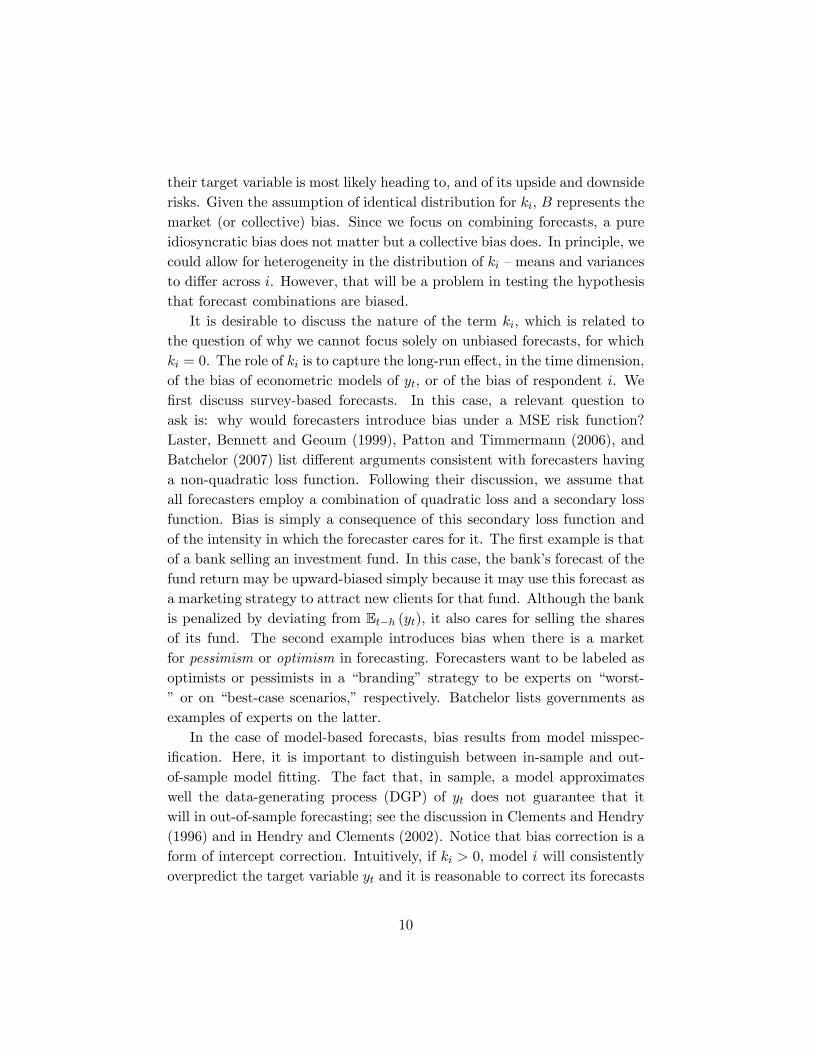
their target variable is most likely heading to, and of its upside and downsiderisks. Given the assumption of identical distribution for ki, B represents themarket (or collective) bias. Since we focus on combining forecasts, a pureidiosyncratic bias does not matter but a collective bias does. In principle, wecould allow for heterogeneity in the distribution of ki �means and variancesto di¤er across i. However, that will be a problem in testing the hypothesisthat forecast combinations are biased.
It is desirable to discuss the nature of the term ki, which is related tothe question of why we cannot focus solely on unbiased forecasts, for whichki = 0. The role of ki is to capture the long-run e¤ect, in the time dimension,of the bias of econometric models of yt, or of the bias of respondent i. We�rst discuss survey-based forecasts. In this case, a relevant question toask is: why would forecasters introduce bias under a MSE risk function?Laster, Bennett and Geoum (1999), Patton and Timmermann (2006), andBatchelor (2007) list di¤erent arguments consistent with forecasters havinga non-quadratic loss function. Following their discussion, we assume thatall forecasters employ a combination of quadratic loss and a secondary lossfunction. Bias is simply a consequence of this secondary loss function andof the intensity in which the forecaster cares for it. The �rst example is thatof a bank selling an investment fund. In this case, the bank�s forecast of thefund return may be upward-biased simply because it may use this forecast asa marketing strategy to attract new clients for that fund. Although the bankis penalized by deviating from Et�h (yt), it also cares for selling the sharesof its fund. The second example introduces bias when there is a marketfor pessimism or optimism in forecasting. Forecasters want to be labeled asoptimists or pessimists in a �branding� strategy to be experts on �worst-� or on �best-case scenarios,� respectively. Batchelor lists governments asexamples of experts on the latter.
In the case of model-based forecasts, bias results from model misspec-i�cation. Here, it is important to distinguish between in-sample and out-of-sample model �tting. The fact that, in sample, a model approximateswell the data-generating process (DGP) of yt does not guarantee that itwill in out-of-sample forecasting; see the discussion in Clements and Hendry(1996) and in Hendry and Clements (2002). Notice that bias correction is aform of intercept correction. Intuitively, if ki > 0, model i will consistentlyoverpredict the target variable yt and it is reasonable to correct its forecasts
10

downwards by the same amount as ki. The equivalence between bias correc-tion and intercept correction was discussed by Hendry and Clements (2002);we discuss this equivalence below. Alternatively, Palm and Zellner (1992)list the following reasons for bias in forecasts: carelessness; the use of a pooror defective information set or incorrect model; and errors of measurement.
Assumption 3 The aggregate shock �t is a stationary and ergodic MAprocess of order at most h� 1, with zero mean and variance �2� <1.
Since h is a bounded constant in our setup, �t is the result of a cumulationof shocks to yt that occurred between t� h+ 1 and t. Being an MA (�) is aconsequence of the wold representation for yt and of (2). If yt is already anMA (�) process, of order smaller than h�1, then, its order will be the same ofthat of �t. Otherwise, the order is h�1. In any case, it must be stressed that�t is unpredictable, i.e., that Et�h (�t) = 0. This a consequence of (2) and ofthe law of iterated expectations, simply showing that, from the perspectiveof the forecast horizon h, unless the forecaster has superior information, theaggregate shock �t cannot be predicted.
Assumption 4: Let "t = ("1;t; "2;t; ::: "N;t)0 be a N � 1 vector stacking the
errors "i;t associated with all possible forecasts, where E ("i;t) = 0 forall i and t. Then, the vector process f"tg is assumed to be covariance-stationary and ergodic for the �rst and second moments, uniformly onN . Further, de�ning as �i;t = "i;t � Et�1 ("i;t), the innovation of "i;t,we assume that
limN!1
1
N2
NXi=1
NXj=1
��E ��i;t�j;t��� = 0: (6)
Because the forecasts are computed h-steps ahead, forecast errors "i;tcan be serially correlated. Assuming that "i;t is weakly stationary is a wayof controlling its time-series dependence. It does not rule out errors dis-playing conditional heteroskedasticity, since the latter can coexist with theassumption of weak stationarity; see Engle (1982).
Equation (6) limits the degree of cross-sectional dependence of the er-rors "i;t. It allows cross-correlation of the form present in a speci�c groupof forecasts, although it requires that this cross-correlation will not pre-vent a weak law-of-large-numbers from holding. Following the forecasting
11
literature with large N and T , e.g., Stock and Watson (2002b), and the�nancial econometric literature, e.g., Chamberlain and Rothschild (1983),the condition lim
N!11N2
PNi=1
PNj=1
��E ��i;t�j;t��� = 0 controls the degree of
cross-sectional decay in forecast errors. It is noted by Bai (2005, p. 6), thatChamberlain and Rothschild�s cross-sectional error decay requires:
limN!1
1
N
NXi=1
NXj=1
��E ��i;t�j;t��� <1: (7)
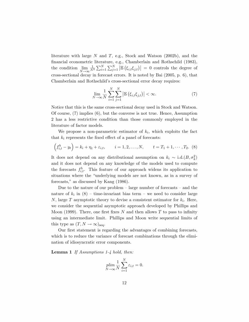
Notice that this is the same cross-sectional decay used in Stock and Watson.Of course, (7) implies (6), but the converse is not true. Hence, Assumption2 has a less restrictive condition than those commonly employed in theliterature of factor models.
We propose a non-parametric estimator of ki, which exploits the factthat ki represents the �xed e¤ect of a panel of forecasts:�fhi;t � yt
�= ki + �t + "i;t; i = 1; 2; : : : ; N; t = T1 + 1; � � � ; T2: (8)
It does not depend on any distributional assumption on ki � i.d.(B; �2k)and it does not depend on any knowledge of the models used to computethe forecasts fhi;t. This feature of our approach widens its application tosituations where the �underlying models are not known, as in a survey offorecasts,�as discussed by Kang (1986).
Due to the nature of our problem �large number of forecasts �and thenature of ki in (8) � time-invariant bias term �we need to consider largeN , large T asymptotic theory to devise a consistent estimator for ki. Here,we consider the sequential asymptotic approach developed by Phillips andMoon (1999). There, one �rst �xes N and then allows T to pass to in�nityusing an intermediate limit. Phillips and Moon write sequential limits ofthis type as (T;N !1)seq.
Our �rst statement is regarding the advantages of combining forecasts,which is to reduce the variance of forecast combinations through the elimi-nation of idiosyncratic error components.
Lemma 1 If Assumptions 1-4 hold, then:
plimN!1
1
N
NXi=1
"i;t = 0:
12
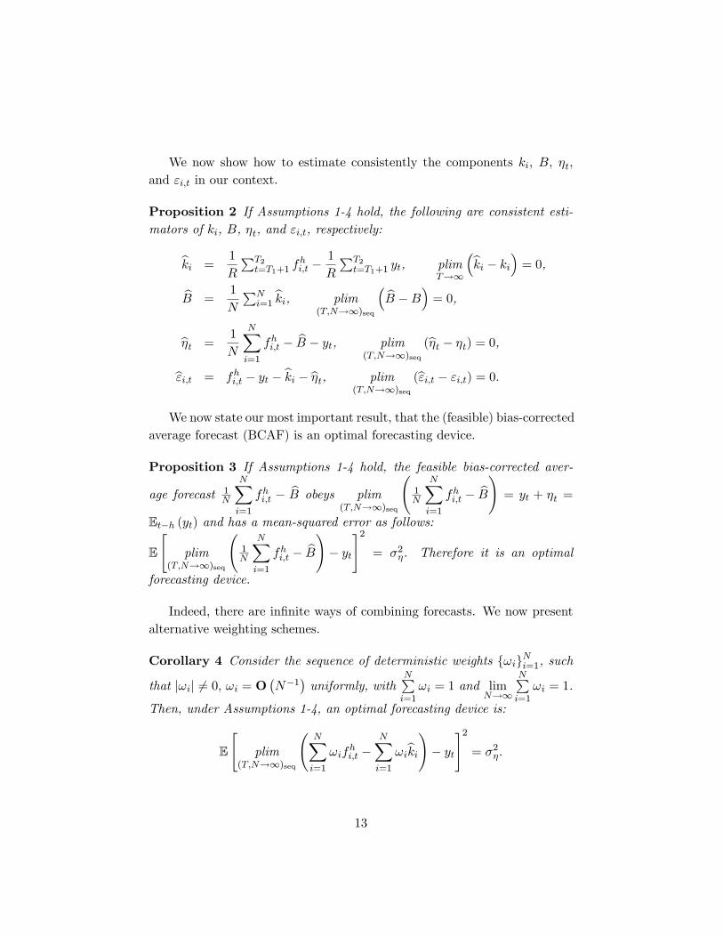
We now show how to estimate consistently the components ki, B, �t,and "i;t in our context.
Proposition 2 If Assumptions 1-4 hold, the following are consistent esti-mators of ki, B, �t, and "i;t, respectively:
bki =1
R
PT2t=T1+1
fhi;t �1
R
PT2t=T1+1
yt, plimT!1
�bki � ki� = 0,bB =
1
N
PNi=1bki, plim
(T;N!1)seq
� bB �B� = 0,b�t =
1
N
NXi=1
fhi;t � bB � yt, plim(T;N!1)seq
(b�t � �t) = 0,b"i;t = fhi;t � yt � bki � b�t, plim
(T;N!1)seq(b"i;t � "i;t) = 0:
We now state our most important result, that the (feasible) bias-correctedaverage forecast (BCAF) is an optimal forecasting device.
Proposition 3 If Assumptions 1-4 hold, the feasible bias-corrected aver-
age forecast 1N
NXi=1
fhi;t � bB obeys plim(T;N!1)seq
1N
NXi=1
fhi;t � bB! = yt + �t =
Et�h (yt) and has a mean-squared error as follows:
E
"plim
(T;N!1)seq
1N
NXi=1
fhi;t � bB!� yt#2 = �2�. Therefore it is an optimal
forecasting device.
Indeed, there are in�nite ways of combining forecasts. We now presentalternative weighting schemes.
Corollary 4 Consider the sequence of deterministic weights f!igNi=1, such
that j!ij 6= 0; !i = O�N�1� uniformly, with NP
i=1!i = 1 and lim
N!1
NPi=1!i = 1.
Then, under Assumptions 1-4, an optimal forecasting device is:
E
"plim
(T;N!1)seq
NXi=1
!ifhi;t �
NXi=1
!ibki!� yt#2 = �2�:
13
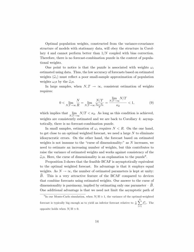
Optimal population weights, constructed from the variance-covariancestructure of models with stationary data, will obey the structure in Corol-lary 4 and cannot perform better than 1=N coupled with bias correction.Therefore, there is no forecast-combination puzzle in the context of popula-tional weights.
One point to notice is that the puzzle is associated with weights !iestimated using data. Thus, the low accuracy of forecasts based on estimatedweights (b!i) must re�ect a poor small-sample approximation of populationweights !is by the b!is.
In large samples, when N;T ! 1, consistent estimation of weightsrequires:
0 < limN;T!1
N
R= limN;T!1
N=TT2�T1T
=
limN;T!1
N=T
�2< 1; (9)
which implies that limN;T!1
N=T < �2. As long as this condition is achieved,
weights are consistently estimated and we are back to Corollary 4: asymp-totically, there is no forecast-combination puzzle.
In small samples, estimation of !i requires N < R. On the one hand,to get close to an optimal weighted forecast, we need a large N to eliminateidiosyncratic errors. On the other hand, the forecast based on estimatedweights is not immune to the �curse of dimensionality:�as N increases, weneed to estimate an increasing number of weights, but this contributes toraise the variance of estimated weights and works against consistency of theb!is. Here, the curse of dimensionality is an explanation to the puzzle9.
Proposition 3 shows that the feasible BCAF is asymptotically equivalentto the optimal weighted forecast. Its advantage is that it employs equalweights. As N !1, the number of estimated parameters is kept at unity:bB. This is a very attractive feature of the BCAF compared to devicesthat combine forecasts using estimated weights. Our answer to the curse ofdimensionality is parsimony, implied by estimating only one parameter � bB.One additional advantage is that we need not limit the asymptotic path of
9 In our Monte-Carlo simulation, when N=R ' 1, the variance of the optimal-weighted
forecast is typically big enough as to yield an inferior forecast relative to 1N
NXi=1
fhi;t. The
opposite holds when N=R ' 0.
14

N;T as in (9), which is the case of forecasts based on estimated weights10.
Remark 5 The optimality result in Proposition 3 is based on fhi;t = Et�h (yt)+ki+"i;t, where the bias ki is additive. Alternatively, if the bias is multiplica-tive as well as additive, i.e., fhi;t = �iEt�h (yt) + ki + "i;t, where �i 6= 1 and�i�
��; �2�
�, the BCAF is no longer optimal if � 6= 1. Optimality can be
restored if the BCAF is slightly modi�ed to be 1N
NPi=1
�fi;tb� � bkib�
�, where .bki
and b� are consistent estimators of ki and �, respectively.Finally, we propose a new test for the usefulness of bias correction (H0 :
B = 0) using the theory of random �elds as in Conley (1999). It is potentiallyrelevant when we view B as amarket or a consensus bias, which is customaryin the �nance and macroeconomics literature, respectively. When B = 0,
the feasible BCAF becomes 1N
NXi=1
fhi;t.
Proposition 6 Under the null hypothesis H0 : B = 0, the test statistic:
bt = bBpbV d�!(T;N!1)seq
N (0; 1) ;
where bV is a consistent estimator of the asymptotic variance of B = 1N
NXi=1
ki.
2.1 The BCAF and Nested Models
It is important to discuss whether and when the techniques above are ap-plicable to the situation where some (or all) of the models we combine arenested. The potential problem is that the innovations from nested mod-els can exhibit high cross-sectional dependence, violating Assumption 4. Inwhat follows, we introduce nested models into our framework in the follow-ing way. Consider a continuous set of models and split the total number
10We must stress that bias-correction can be viewed as a form of intercept correctionas discussed in Palm and Zellner (1992) and Hendry and Mizon (2005), for example. Wecould retrieve bB from an OLS regression of the form: y = �i+!1f1+!2f2+ :::+!NfN+�,where the weights !i are constrained to be !i = 1=N for all i. There is only one parameterto be estimated, �, and b� = � bB, where bB is now cast in terms of the previous literature
15
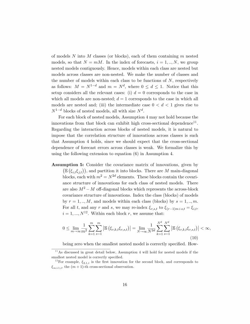
of models N into M classes (or blocks), each of them containing m nestedmodels, so that N = mM . In the index of forecasts, i = 1; ::; N , we groupnested models contiguously. Hence, models within each class are nested butmodels across classes are non-nested. We make the number of classes andthe number of models within each class to be functions of N , respectivelyas follows: M = N1�d and m = Nd, where 0 � d � 1. Notice that thissetup considers all the relevant cases: (i) d = 0 corresponds to the case inwhich all models are non-nested; d = 1 corresponds to the case in which allmodels are nested and; (iii) the intermediate case 0 < d < 1 gives rise toN1�d blocks of nested models, all with size Nd.
For each block of nested models, Assumption 4 may not hold because theinnovations from that block can exhibit high cross-sectional dependence11.Regarding the interaction across blocks of nested models, it is natural toimpose that the correlation structure of innovations across classes is suchthat Assumption 4 holds, since we should expect that the cross-sectionaldependence of forecast errors across classes is weak. We formalize this byusing the following extension to equation (6) in Assumption 4.
Assumption 5: Consider the covariance matrix of innovations, given by�E��i;t�j;t
��, and partition it into blocks. There are M main-diagonal
blocks, each withm2 = N2d elements. These blocks contain the covari-ance structure of innovations for each class of nested models. Thereare also M2�M o¤-diagonal blocks which represents the across-blockcovariance structure of innovations. Index the class (blocks) of modelsby r = 1; ::;M , and models within each class (blocks) by s = 1; ::;m.For all t, and any r and s, we may re-index �r;s;t to �(r�1)m+s;t = �i;t,i = 1; :::; N 12. Within each block r, we assume that:
0 � limm!1
1
m2
mXk=1
mXs=1
��E ��r;k;t�r;s;t��� = limN!1
1
N2d
NdXk=1
NdXs=1
��E ��r;k;t�r;s;t��� <1;(10)
being zero when the smallest nested model is correctly speci�ed. How-
11As discussed in great detail below, Assumption 4 will hold for nested models if thesmallest nested model is correctly speci�ed.12For example, �2;1;t is the �rst innovation for the second block, and corresponds to
�m+1;t, the (m+ 1)-th cross-sectional observation.
16
ever, across any two blocks r and l, r 6= l, we assume that:
limm!1
1
m2
mXk=1
mXs=1
��E ��r;k;t�l;s;t��� = limN!1
1
N2d
NdXk=1
NdXs=1
��E ��r;k;t�l;s;t��� = 0:(11)
We now discuss how to implement the BCAF in the presence of nestedmodels. The matrix
�E��i;t�j;t
��has N2 = m2M2 elements, but only
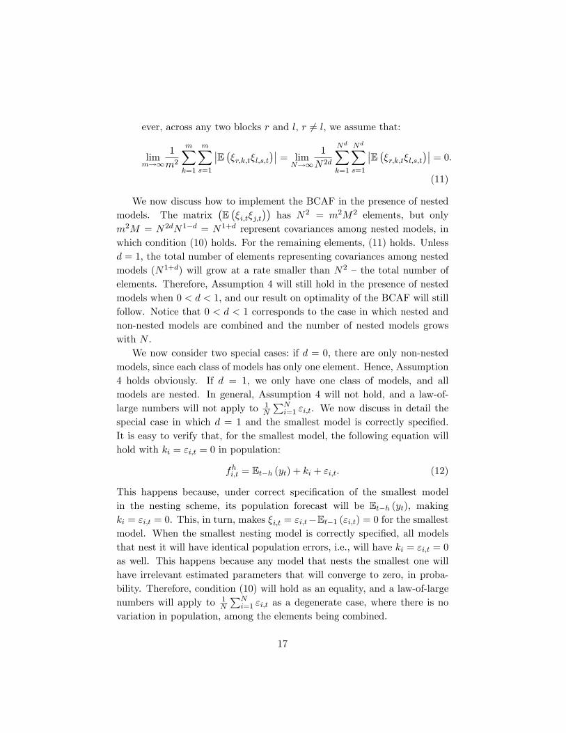
m2M = N2dN1�d = N1+d represent covariances among nested models, inwhich condition (10) holds. For the remaining elements, (11) holds. Unlessd = 1, the total number of elements representing covariances among nestedmodels (N1+d) will grow at a rate smaller than N2 �the total number ofelements. Therefore, Assumption 4 will still hold in the presence of nestedmodels when 0 < d < 1, and our result on optimality of the BCAF will stillfollow. Notice that 0 < d < 1 corresponds to the case in which nested andnon-nested models are combined and the number of nested models growswith N .
We now consider two special cases: if d = 0, there are only non-nestedmodels, since each class of models has only one element. Hence, Assumption4 holds obviously. If d = 1, we only have one class of models, and allmodels are nested. In general, Assumption 4 will not hold, and a law-of-large numbers will not apply to 1
N
PNi=1 "i;t. We now discuss in detail the
special case in which d = 1 and the smallest model is correctly speci�ed.It is easy to verify that, for the smallest model, the following equation willhold with ki = "i;t = 0 in population:
fhi;t = Et�h (yt) + ki + "i;t. (12)
This happens because, under correct speci�cation of the smallest modelin the nesting scheme, its population forecast will be Et�h (yt), makingki = "i;t = 0. This, in turn, makes �i;t = "i;t�Et�1 ("i;t) = 0 for the smallestmodel. When the smallest nesting model is correctly speci�ed, all modelsthat nest it will have identical population errors, i.e., will have ki = "i;t = 0as well. This happens because any model that nests the smallest one willhave irrelevant estimated parameters that will converge to zero, in proba-bility. Therefore, condition (10) will hold as an equality, and a law-of-largenumbers will apply to 1
N
PNi=1 "i;t as a degenerate case, where there is no
variation in population, among the elements being combined.
17

From an empirical point of view, d can be regarded as choice variablewhen implementing the BCAF. Choosing d = 1 (only one class of nestedmodels) is an �excellent�choice when the class of model chosen is correctlyspeci�ed (the smallest model is correctly speci�ed). However, there is the(potentially high) risk of incorrect speci�cation for the whole class, whichwill imply that the law-of-large numbers will not hold for 1
N
PNi=1 "i;t in im-
plementing the BCAF. On the other hand, in choosing d = 0 (all models arenon-nested), we completely eliminate nested models and the chance that thelaw-of-large numbers will not hold. In the intermediate case, 0 < d < 1, wehave nested models but can still apply a law-of-large numbers for 1
N
PNi=1 "i;t
and implement the BCAF successfully. Here, keeping some nested modelsposes no problem at all, since the mixture of models will still deliver the op-timal forecast. From a practical point of view, the choice of 0 � d < 1 seemsto be superior. Here, we are back to the main theorem in �nance about riskdiversi�cation: do not put all your eggs in the same basket, choosing a largeenough number of diversi�ed (classes of) models.
3 Monte-Carlo Study
3.1 Experiment design
We follow the setup presented in the theoretical part of this paper in whicheach forecast is the conditional expectation of the target variable plus an ad-ditive bias term and an idiosyncratic error. Our DGP is a simple stationaryAR(1) process:
yt = �0 + �1yt�1 + �t, t = 1; :::T1; :::; T2; :::; T (13)
�t � i.i.d.N(0; 1), �0 = 0, and �1 = 0:5,
where �t is an unpredictable aggregate zero-mean shock. We focus on one-step-ahead forecasts for simplicity. The conditional expectation of yt isEt�1 (yt) = �0 + �1yt�1. Since �t is unpredictable, the forecaster shouldbe held accountable for fi;t � Et�1 (yt). These deviations have two terms:the individual speci�c biases (ki) and the idiosyncratic or group error terms("i;t). Because �t �i.i.d.N(0; 1), the optimal theoretical MSE is unity in thisexercise.
18

The conditional expectation Et�1 (yt) = �0 + �1yt�1 is estimated usinga sample of size 200, i.e., E = T1 = 200, so that b�0 ' �0 and b�1 ' �1: Inpractice, however, forecasters may have economic incentives to make biasedforecasts, and there may be other sources of misspeci�cation arising frommisspeci�cation errors. Therefore, we generate forecasts as:
fi;t = b�0 + b�1yt�1 + ki + "i;t; (14)
= (b�0 + ki) + b�1yt�1 + "i;t for t = T1 + 1; � � � ; T , i = 1; :::N;where, ki = �ki�1 + ui, ui �i.i.d.Uniform(a; b), 0 < � < 1, and "t =("1;t; "2;t; ::: "N;t)
0, N � 1, is drawn from a multivariate Normal distributionwith size R + P = T � T1, whose mean vector equals zero and covariancematrix equals �. We introduce heterogeneity and spatial dependence in thedistribution of "i;t. The diagonal elements of � = (�ij) obey: 1 < �ii <
p10,
and o¤-diagonal elements obey: �ij = 0:5, if ji� jj = 1, �ij = 0:25, ifji� jj = 2, and �ij = 0, if ji� jj > 2. The exact values of the �ii�sare randomly determined through an once-and-for-all draw from a uniformrandom variable of size N , that is, �ii �i.i.d.Uniform(1;
p10)13.
In equation (14), we built spatial dependence in the bias term ki14. The
cross-sectional average of ki is a+b2(1��) . We set the degree of spatial depen-
dence in ki by letting � = 0:5. For the support of ui, we consider two cases:(i) a = 0 and b = 0:5 and; (ii) a = �0:5 and b = 0:5. This implies that theaverage bias is B = 0:5 in (i), whereas it is B = 0 in (ii). Finally, notice thatthe speci�cation of "i;t satis�es Assumption 4 in Section 2 as we let N !1.
Equation (14) is used to generate di¤erent panels of forecasts in terms ofthe number of forecasters (N) and the size of the training-sample (R). Wekept the number of out-of-sample observations equal to P = 50 in all cases.First, for N = 10; 20; 40, we let R = 50. For all these 3 cases, NR may notbe small enough to guarantee a good approximation of optimal populationweights by the b!is. In order to approximate the asymptotic environmentneeded for optimality of the forecasts based on estimated weights, we also13The covariance matrix � does not change over simulations.14The additive bias ki is explicit in (14). It could be implicit if we had considered
a structural break in the target variable as did Hendry and Clements (2002). There,an intercept change in yt takes place right after the estimation of econometric models,biasing all forecasts. Hence, in their paper, intercept correction is equivalent to biascorrection, which would be the case here too. However, a structural break would violateweak stationarity and that is why it is not attempted here.
19

considered the case in which R = 500, and 1; 000, while keeping N = 10. Foreach N , we conducted 50; 000 simulations in the experiment. In all cases, thetotal number of time observations used to �t models equals E = T1 = 200.
3.2 Forecast approaches
In our simulations, we evaluate three forecasting methods: the feasible bias-corrected average forecast (BCAF), the forecast based on estimated weights,and the forecast based on �xed weights. For these methods, our resultsinclude aspects of the whole distribution of their respective biases and MSEs.
For the BCAF, we use the training-sample observations to estimate bki =1R
T2Pt=T1+1
(yt � fi;t) and bB = 1N
NPi=1
bki. Then, we compute the out-of-sampleforecasts bfBCAFt = 1
N
NPi=1fi;t � bB, t = T2 + 1; :::; T , and we employ the last
P observations to compute MSEBCAF = 1P
TPt=T2+1
�yt � bfBCAFt
�2.
For the forecast based on estimated weights (weighted average forecast),we use R observations of the training sample to estimate weights (!i) byOLS in:
y = �i+ !1f1 + !2f2 + :::+ !NfN + ",
where the restrictionNXi=1
!i = 1 is imposed in estimation. The weighted
forecast is bfweightedt = b� + b!1f1;t + b!2f2;t + ::: + b!NfN;t, and the intercept� plays the role of bias correction. We employ the last P observations to
compute MSEweighted = 1P
TPt=T2+1
�yt � bfweightedt
�2.
For the forecast based on �xed weights (average forecast), there is no pa-rameter to be estimated using training-sample observations. Out-of-sample
forecasts are computed according to faveraget = 1N
NPi=1fi;t, t = T2 + 1; :::; T ,
and its MSE is computed as MSEaverage = 1P
TPt=T2+1
(yt � faveraget )2.
Finally, for each approach, we also computed the out-of-sample meanbiases. In small samples, the weighted forecast and the BCAF should haveout-of-sample mean biases close to zero, whereas the mean bias of the averageforecast should be close to B = a+b
2(1��) .
20

3.3 Simulation Results
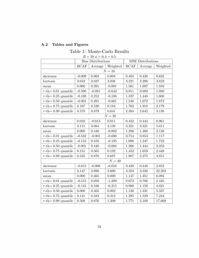
With the results of the 50; 000 replications, we describe the empirical dis-tributions of the bias and the MSE of all three forecasting methods. Foreach distribution we compute the following statistics: (i) kurtosis; (ii) skew-ness, and (iii) � -th unconditional quantile, with � = 0:01; 0:25; 0:50; 0:75;
and 0:99. In doing so, we seek to have a general description of all threeforecasting approaches.
The main results are presented in Tables 1 through 4. In Table 1, whereB = 0:5, the average bias across simulations of the BCAF and the weightedforecast combination are practically zero. The mean bias of the simpleaverage forecast is between 0:39 and 0:46, depending onN . In terms of MSE,the BCAF performs very well compared to the other two methods. Thesimple average forecast has a mean MSE at least 8:7% higher than that of thebias-corrected average forecast, reaching 17:8% higher when N = 40. Theforecast based on estimated weights has an mean MSE at least 22:7% higher,reaching 431:3% higher when N = 40. This last result is a consequence ofthe increase in variance as we increase N , with R �xed, and N=R close tounity. Notice that the average bias is virtually zero for N = 10; 20; 40. Sincethe MSE triples when N is increased from 10 to 40, all the increase in MSEis due to variance, revealing the curse-of-dimensionality working against theforecast based on estimated weights.
Table 2 presents the results when B = 0. In this case, the optimalforecast is the simple average, since there is no need to estimate a bias-correction term. In terms of MSE, comparing the simple-average forecastwith the BCAF, we observe that they are almost identical �the mean MSEof the BCAF is about 1% higher than that of the average forecast, showingthat not much is lost in terms of MSE when we perform an unwanted biascorrection. The behavior of the weighted average forecast is identical to thatin Table 1.
Table 3 presents the result in which B = 0:5, NR � 0, and N = 10, withR = 500; 1; 000. As expected, the b!is are a very good approximation to opti-mal population weights. Despite that, we are still combining a relatively lownumber of forecasts: N = 10. Here, there is practically no di¤erence in per-formance between the BCAF and the estimated-weight forecast. However,contrary to the results in Tables 1 and 2, equal-weight forecasts perform
21
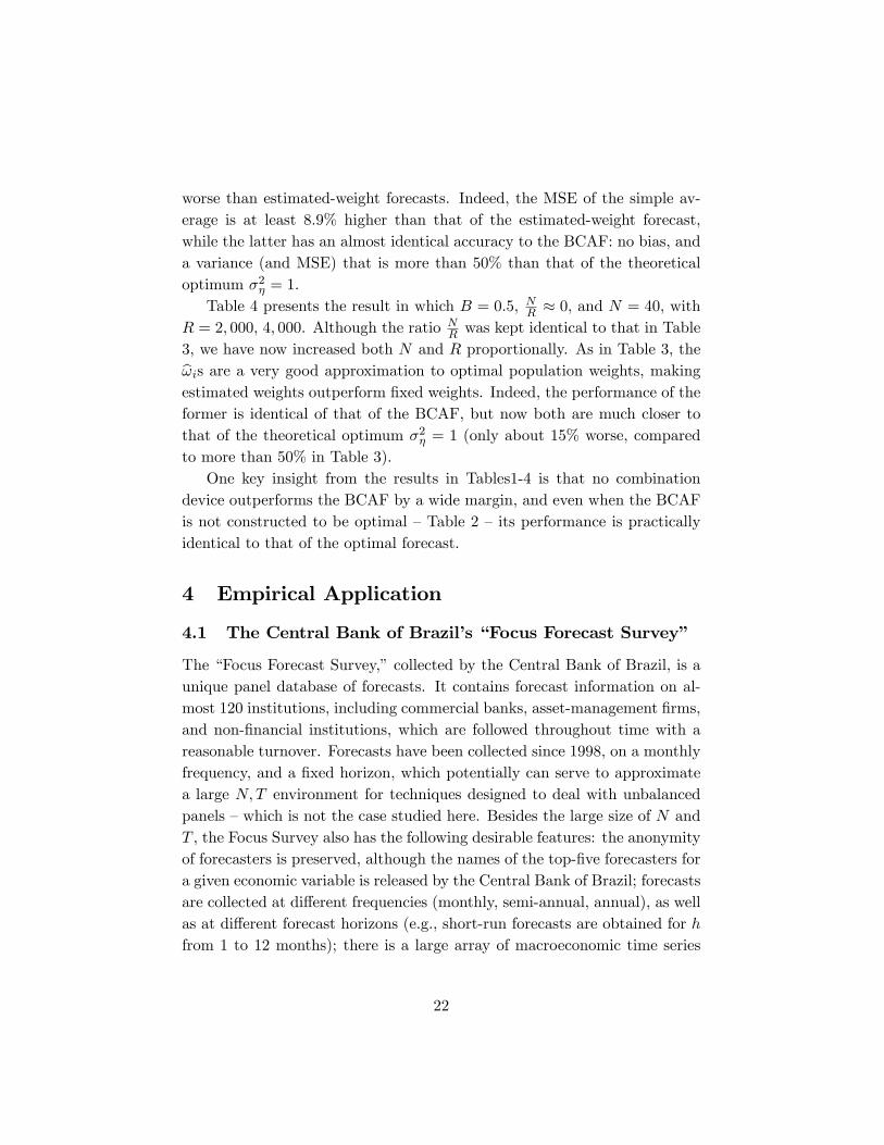
worse than estimated-weight forecasts. Indeed, the MSE of the simple av-erage is at least 8:9% higher than that of the estimated-weight forecast,while the latter has an almost identical accuracy to the BCAF: no bias, anda variance (and MSE) that is more than 50% than that of the theoreticaloptimum �2� = 1.
Table 4 presents the result in which B = 0:5, NR � 0, and N = 40, withR = 2; 000; 4; 000. Although the ratio N
R was kept identical to that in Table3, we have now increased both N and R proportionally. As in Table 3, theb!is are a very good approximation to optimal population weights, makingestimated weights outperform �xed weights. Indeed, the performance of theformer is identical of that of the BCAF, but now both are much closer tothat of the theoretical optimum �2� = 1 (only about 15% worse, comparedto more than 50% in Table 3).
One key insight from the results in Tables1-4 is that no combinationdevice outperforms the BCAF by a wide margin, and even when the BCAFis not constructed to be optimal �Table 2 �its performance is practicallyidentical to that of the optimal forecast.
4 Empirical Application
4.1 The Central Bank of Brazil�s �Focus Forecast Survey�
The �Focus Forecast Survey,�collected by the Central Bank of Brazil, is aunique panel database of forecasts. It contains forecast information on al-most 120 institutions, including commercial banks, asset-management �rms,and non-�nancial institutions, which are followed throughout time with areasonable turnover. Forecasts have been collected since 1998, on a monthlyfrequency, and a �xed horizon, which potentially can serve to approximatea large N;T environment for techniques designed to deal with unbalancedpanels �which is not the case studied here. Besides the large size of N andT , the Focus Survey also has the following desirable features: the anonymityof forecasters is preserved, although the names of the top-�ve forecasters fora given economic variable is released by the Central Bank of Brazil; forecastsare collected at di¤erent frequencies (monthly, semi-annual, annual), as wellas at di¤erent forecast horizons (e.g., short-run forecasts are obtained for hfrom 1 to 12 months); there is a large array of macroeconomic time series
22

included in the survey.To save space, we focus our analysis on the behavior of forecasts of the
monthly in�ation rate in Brazil (�t), in percentage points, as measured bythe o¢ cial Consumer Price Index (CPI), computed by FIBGE. In orderto obtain the largest possible balanced panel (N � T ), we used N = 18
and a time-series sample period covering 2002:11 through 2006:3 (T = 41).Of course, in the case of a survey panel, there is no estimation sample.We chose the �rst R = 26 time observations to compute bB �the averagebias � leaving P = 18 time-series observations for out-of-sample forecastevaluation. The forecast horizon chosen was h = 6, this being an importanthorizon to determine future monetary policy within the Brazilian In�ation-Targeting program.
The results of our empirical exercise are presented in Tables 5 and 6.First, we note that all the 18 individual forecasts perform worse than com-binations, which is consistent with the discussion in Hendry and Clements(2002). The results in Table 5 show that the average bias is positive for the 6-month horizon, 0:06187, and marginally signi�cant, with a p-value of 0:063.This is a sizable bias �approximately 0:75 percentage points in a yearly ba-sis, for an average in�ation rate of 5:27% a year. In Table 6, out-of-sampleforecast comparisons between the simple average and the bias-corrected av-erage forecast show that the former has a MSE 18:2% bigger than that ofthe latter. We also computed the MSE of the weighted forecast. Since wehave N = 18 and R = 26, N=R = 0:69. Hence, the weighted average cannotavoid the curse of dimensionality, yielding a MSE 390:2% bigger than thatof the BCAF.
It is important to stress that, although the bias-corrected average fore-cast was conceived for a large N;T environment, the empirical results hereshow an encouraging performance even in a small N;T context. Also, theforecasting gains from bias correction are non-trivial.
5 Conclusions and Extensions
In this paper, we propose a novel approach to econometric forecast of station-ary and ergodic series yt within a panel-data framework, where the numberof forecasts and the number of time periods increase without bounds. Thebasis of our method is a two-way decomposition of the forecasts error. As
23

shown here, this is equivalent to forecasters trying to approximate the op-timal forecast under quadratic loss �the conditional expectation Et�h (yt),which is modelled as the common feature of all individual forecasts. Stan-dard tools from panel-data asymptotic theory are used to devise an optimalforecasting combination that delivers Et�h (yt). This optimal combinationuses equal weights and an estimated bias-correction term. The use of equalweights avoids estimating forecast weights, which contributes to reduce fore-cast variance, although potentially at the cost of an increase in bias. Theuse of an estimated bias-correction term eliminates any possible detrimentale¤ect arising from equal weighting. We label this optimal forecast as the(feasible) bias-corrected average forecast.
We show that the BCAF delivers the optimality result even under thepresence of nested models and we fully characterize it by using a novel frame-work. As a by-product of the use of panel-data asymptotic methods, withN;T !1, we advanced the understanding of the forecast combination puz-zle by showing that the low accuracy of the forecasts based on estimatedweights relative to those based on �xed weights re�ect a poor small-sampleapproximation of optimal population weights !is by estimated weights. Insmall samples, estimation of !i requires N < R. On the one hand, to getclose to an optimal weighted forecast, we need a large N . On the otherhand, the forecast based on estimated weights is not immune to the �curseof dimensionality,�since, as N increases, we need to estimate an increasingnumber of weights. Our simulations, we show that the curse of dimensional-ity works against forecast based on estimated weights, increasing their MSEwhen N approaches R.
Finally, we show that there is no forecast-combination puzzle under cer-tain asymptotic paths for N and T , but not for all. Indeed, if N ! 1at a rate strictly smaller than T , then, !i is consistently estimated, theweighted forecast with bias correction (intercept) is optimal, and there isno puzzle. Our simulations approximate this asymptotic environment byconsidering various cases in which N=T � 0. As expected, the forecastbased on estimated weights outperform the simple �xed-weight combina-tion and has the same performance as the BCAF. Since the case in whichN=T � 0 is rarely observed in practice, we should not expect forecasts basedon estimated-weight combinations to be accurate. On the other hand, BCAFis asymptotically equivalent to the optimal-weighted forecast but has a su-
24

perior performance in small samples.
References
[1] Amemiya, T. (1971), �The estimation of the variances in the variance-components model�, International Economic Review, vol. 12, pp. 1-13.
[2] Baltagi, Badi H., 1980, �On Seemingly Unrelated Regressions with Er-ror Components,�Econometrica, Vol. 48(6), pp. 1547-1551.
[3] Bai, J., (2005), �Panel Data Models with Interactive Fixed E¤ects,�Working Paper: New York University.
[4] Bai, J., and S. Ng, (2002), �Determining the Number of Factors inApproximate Factor Models,�Econometrica, 70, 191-221.
[5] Bates, J.M. and Granger, C.W.J., 1969, �The Combination of Fore-casts,�Operations Research Quarterly, vol. 20, pp. 309-325.
[6] Batchelor, R., 2007, �Bias in macroeconomic forecasts,� InternationalJournal of Forecasting, vol. 23, pp. 189�203.
[7] Chamberlain, Gary, and Rothschild, Michael, (1983). �Arbitrage, Fac-tor Structure, and Mean-Variance Analysis on Large Asset Markets,�Econometrica, vol. 51(5), pp. 1281-1304.
[8] Clements, M.P. and D.F. Hendry, 2006, Forecasting with Breaks in DataProcesses, in C.W.J. Granger, G. Elliott and A. Timmermann (eds.)Handbook of Economic Forecasting, pp. 605-657, Amsterdam, North-Holland.
[9] Conley, T.G., 1999, �GMM Estimation with Cross Sectional Depen-dence,�Journal of Econometrics, Vol. 92 Issue 1, pp. 1-45.
[10] Connor, G., and R. Korajzcyk (1986), �Performance Measurement withthe Arbitrage Pricing Theory: A New Framework for Analysis,�Journalof Financial Economics, 15, 373-394.
[11] Davies, A. and Lahiri, K., 1995, �A new framework for analyzing surveyforecasts using three-dimensional panel data,�Journal of Econometrics,vol. 68(1), pp. 205-227
25

[12] Elliott, G., C.W.J. Granger, and A. Timmermann, 2006, Editors, Hand-book of Economic Forecasting, Amsterdam: North-Holland.
[13] Elliott, G. and A. Timmermann (2005), �Optimal forecast combina-tion weights under regime switching�, International Economic Review,46(4), 1081-1102.
[14] Elliott, G. and A. Timmermann (2004), �Optimal forecast combina-tions under general loss functions and forecast error distributions�,Journal of Econometrics 122:47-79.
[15] Engle, R.F. (1982), �Autoregressive Conditional Heteroskedasticitywith Estimates of the Variance of United Kingdom In�ation,�Econo-metrica, 50, pp. 987-1006.
[16] Engle, R.F. and Kozicki, S. (1993). �Testing for Common Features�,Journal of Business and Economic Statistics, 11(4): 369-80.
[17] Forni, M., Hallim, M., Lippi, M. and Reichlin, L. (2000), �The Gener-alized Dynamic Factor Model: Identi�cation and Estimation�, Reviewof Economics and Statistics, 2000, vol. 82, issue 4, pp. 540-554.
[18] Forni M., Hallim M., Lippi M. and Reichlin L., 2003 �The GeneralizedDynamic Factor Model one-sided estimation and forecasting,�Journalof the American Statistical Association, forthcoming.
[19] Fuller, Wayne A. and George E. Battese, 1974, �Estimation of linearmodels with crossed-error structure,� Journal of Econometrics, Vol.2(1), pp. 67-78.
[20] Granger, C.W.J., 1989, �Combining Forecasts-Twenty Years Later,�Journal of Forecasting, vol. 8, 3, pp. 167-173.
[21] Granger, C.W.J., and R. Ramanathan (1984), �Improved methods ofcombining forecasting�, Journal of Forecasting 3:197�204.
[22] Hendry, D.F. and M.P. Clements (2002), �Pooling of forecasts�, Econo-metrics Journal, 5:1-26.
[23] Hendry, D.F. and Mizon, G.E. (2005): �Forecasting in the Presenceof Structural Breaks and Policy Regime Shifts�, in �Identi�cation and
26

Inference for Econometric Models: Essays in Honor of Thomas Rothen-berg,�D.W.K. Andrews and J.H. Stock (eds.), Cambridge UniversityPress.
[24] Issler, J. V., Vahid, F., 2001, �Common cycles and the importance oftransitory shocks to macroeconomic aggregates,�Journal of MonetaryEconomics, vol. 47, 449�475.
[25] Issler, J. V., Vahid, F., 2006, �The missing link: Using the NBER reces-sion indicator to construct coincident and leading indices of economicactivity,� Annals Issue of the Journal of Econometrics on CommonFeatures, vol. 132(1), pp. 281-303.
[26] Kang, H. (1986), �Unstable Weights in the Combination of Forecasts,�Management Science 32, 683-95.
[27] Laster, David, Paul Bennett and In Sun Geoum, 1999, �Rational BiasIn Macroeconomic Forecasts,� The Quarterly Journal of Economics,vol. 114, issue 1, pp. 293-318.
[28] Palm, Franz C. and Arnold Zellner, 1992, �To combine or not to com-bine? issues of combining forecasts,� Journal of Forecasting, Volume11, Issue 8 , pp. 687-701.
[29] Patton, Andrew J. and Allan Timmermann, 2006, �Testing ForecastOptimality under Unknown Loss,� forthcoming in the Journal of theAmerican Statistical Association.
[30] Pesaran, M.H., (2005), �Estimation and Inference in Large Hetero-geneous Panels with a Multifactor Error Structure.�Working Paper:Cambridge University, forthcoming in Econometrica.
[31] Phillips, P.C.B. and H.R. Moon, 1999, �Linear Regression Limit Theoryfor Nonstationary Panel Data,�Econometrica, vol. 67 (5), pp. 1057�1111.
[32] Stock, J. and Watson, M., �Forecasting In�ation�, Journal of MonetaryEconomics, 1999, Vol. 44, no. 2.
27
[33] Stock, J. and Watson, M., �Macroeconomic Forecasting Using Di¤usionIndexes�, Journal of Business and Economic Statistics, April 2002a,Vol. 20 No. 2, 147-162.
[34] Stock, J. and Watson, M., �Forecasting Using Principal Componentsfrom a Large Number of Predictors,�Journal of the American Statis-tical Association, 2002b.
[35] Stock, J. andWatson, M., 2006, �Forecasting with Many Predictors,�In:Elliott, G., C.W.J. Granger, and A. Timmermann, 2006, Editors, Hand-book of Economic Forecasting, Amsterdam: North-Holland, Chapter 10,pp. 515-554.
[36] Timmermann, A., 2006, �Forecast Combinations,� in Elliott, G.,C.W.J. Granger, and A. Timmermann, 2006, Editors, Handbook ofEconomic Forecasting, Amsterdam: North-Holland, Chapter 4, pp. 135-196.
[37] Vahid, F. and Engle, R. F., 1993, �Common trends and common cy-cles,�Journal of Applied Econometrics, vol. 8, 341�360.
[38] Vahid, F., Engle, R. F., 1997, �Codependent cycles,�Journal of Econo-metrics, vol. 80, 199�221.
[39] Vahid, F., Issler, J. V., 2002, �The importance of common cyclical fea-tures in VAR analysis: A Monte Carlo study,�Journal of Econometrics,109, 341�363.
[40] Wallace, H. D., Hussain, A., 1969, �The use of error components modelin combining cross-section and time-series data,�Econometrica, 37, 55�72.
[41] West, K., 1996, �Asymptotic Inference about Predictive Ability,�Econometrica, 64, (5), pp. 1067-84.
28
A Appendix
A.1 Proofs of Lemma and Propositions in Section 2
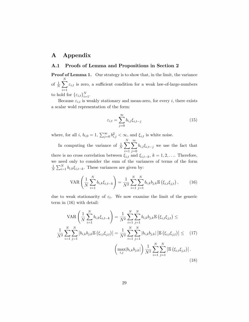
Proof of Lemma 1. Our strategy is to show that, in the limit, the variance
of 1N
NXi=1
"i;t is zero, a su¢ cient condition for a weak law-of-large-numbers
to hold for f"i;tgNi=1.Because "i;t is weakly stationary and mean-zero, for every i, there exists
a scalar wold representation of the form:
"i;t =1Xj=0
bi;j�i;t�j (15)
where, for all i, bi;0 = 1,P1j=0 b
2i;j <1, and �i;t is white noise.
In computing the variance of 1N
NXi=1
1Xj=0
bi;j�i;t�j we use the fact that
there is no cross correlation between �i;t and �i;t�k, k = 1; 2; : : :. Therefore,we need only to consider the sum of the variances of terms of the form1N
PNi=1 bi;k�i;t�k. These variances are given by:
VAR
1
N
NXi=1
bi;k�i;t�k
!=
1
N2
NXi=1
NXj=1
bi;kbj;kE��i;t�j;t
�; (16)
due to weak stationarity of "t. We now examine the limit of the genericterm in (16) with detail:
VAR
1
N
NXi=1
bi;k�i;t�k
!=
1
N2
NXi=1
NXj=1
bi;kbj;kE��i;t�j;t
��
1
N2
NXi=1
NXj=1
��bi;kbj;kE ��i;t�j;t��� = 1
N2
NXi=1
NXj=1
jbi;kbj;kj��E ��i;t�j;t��� � (17)
�maxi;jjbi;kbj;kj
�1
N2
NXi=1
NXj=1
��E ��i;t�j;t��� :(18)
29

Hence:
limN!1
VAR
1
N
NXi=1
bi;k�i;t�k
!� lim
N!1
�maxi;jjbi;kbj;kj
��
limN!1
1
N2
NXi=1
NXj=1
��E ��i;t�j;t��� = 0;
since the sequence fbi;jg1j=0 is square-summable, yielding limN!1
�maxi;jjbi;kbj;kj
�<
1, and Assumption 4 imposes limN!1
1N2
PNi=1
PNj=1
��E ��i;t�j;t��� = 0.Thus, all variances are zero in the limit, as well as their sum, which gives:
plimN!1
1
N
NXi=1
"i;t = 0:
Proof of Proposition 2. Although yt; �t and "i;t are ergodic for the mean,fhi;t is non ergodic because of ki. Recall that, T1; T2; R ! 1, as T ! 1.Then, as T !1,1
R
PT2t=T1+1
fhi;t =1
R
PT2t=T1+1
yt +1
R
PT2t=T1+1
"i;t +1
R
PT2t=T1+1
�t + ki
p! E (yt) + ki + E ("i;t) + E (�t)= E (yt) + ki
Given that we observe fhi;t and yt, we propose the following consistent esti-mator for ki, as T !1:
bki =1
R
PT2t=T1+1
fhi;t �1
R
PT2t=T1+1
yt, i = 1; :::; N
=1
R
PT2t=T1+1
(yt + ki + �t + "i;t)�1
R
PT2t=T1+1
yt
= ki +1
R
PT2t=T1+1
"i;t +1
R
PT2t=T1+1
�t
or,bki � ki =1
R
PT2t=T1+1
"i;t +1
R
PT2t=T1+1
�t:
Using this last result, we can now propose a consistent estimator for B:
bB = 1
N
PNi=1bki = 1
N
PNi=1
�1
R
PT2t=T1+1
fhi;t �1
R
PT2t=T1+1
yt
�.
30

First let T !1,
bki p! ki, and,
1
N
NXi=1
bki p! 1
N
NXi=1
ki.
Now, as N !1, after T !1,
1
N
NXi=1
kip! B;
Hence, as (T;N !1)seq,
plim(T;N!1)seq
� bB �B� = 0:We can now propose a consistent estimator for �t:
b�t = 1
N
NXi=1
fhi;t � bB � yt = 1
N
NXi=1
fhi;t �1
N
NXi=1
bki � yt.We let T !1 to obtain:
plimT!1
1
N
NXi=1
fhi;t �1
N
NXi=1
bki � yt! =1
N
NXi=1
fhi;t �1
N
NXi=1
ki � yt
= �t +1
N
NXi=1
"i;t:
Letting now N !1, we obtain plimN!1
1N
NXi=1
"i;t = 0 and:
plim(T;N!1)seq
(b�t � �t) = 0:Finally,
b"i;t = fhi;t � yt � bki � b�t, and fhi;t � yt = ki + �t + "i;t.Hence :b"i;t � "i;t =
�ki � bki�+ (�t � b�t) :
31

Using the previous results that plimT!1
�bki � ki� = 0 and plim(T;N!1)seq
(b�t � �t) =0, we obtain:
plim(T;N!1)seq
(b"i;t � "i;t) = 0:Proof of Proposition 3. We let T !1 �rst to obtain:
plimT!1
1
N
NXi=1
fhi;t � bB! = plimT!1
1
N
NXi=1
fhi;t �1
N
NXi=1
bki!
=1
N
NXi=1
fhi;t �1
N
NXi=1
ki = yt + �t +1
N
NXi=1
"i;t:
Letting now N !1 we obtain plimN!1
1N
NXi=1
"i;t = 0 and:
plim(T;N!1)seq
1
N
NXi=1
fhi;t � bB! = yt + �t = Et�h (yt) ;from (2) and (3), which is the optimal forecast. The MSE of the feasibleBCAF is:
E
"plim
(T;N!1)seq
1
N
NXi=1
fhi;t � bB!� yt#2 = �2�:Proof of Proposition 4. Under H0 : B = 0, we have shown in Proposi-tion 2 that bB is a (T;N !1)seq consistent estimator for B. To compute theconsistent estimator of the asymptotic variance of B we follow Conley(1999),who matches spatial dependence to a metric of economic distance. Denoteby MSEi (�) and MSEj (�) the MSE in forecasting of forecasts i and j re-spectively. For any two generic forecasts i and j, we use MSEi (�)�MSEj (�)as a measure of distance between these two forecasts. For N forecasts, wecan choose one of them to be the benchmark, say, the �rst one, comput-ing MSEi (�)�MSE1 (�) for i = 2; 3; � � � ; N . With this measure of spatialdependence at hand, we can construct a two-dimensional estimator of theasymptotic variance of B and bB following Conley(1999, Sections 3 and 4).We label V and bV the estimates of the asymptotic variances of B and of bB,respectively.
32
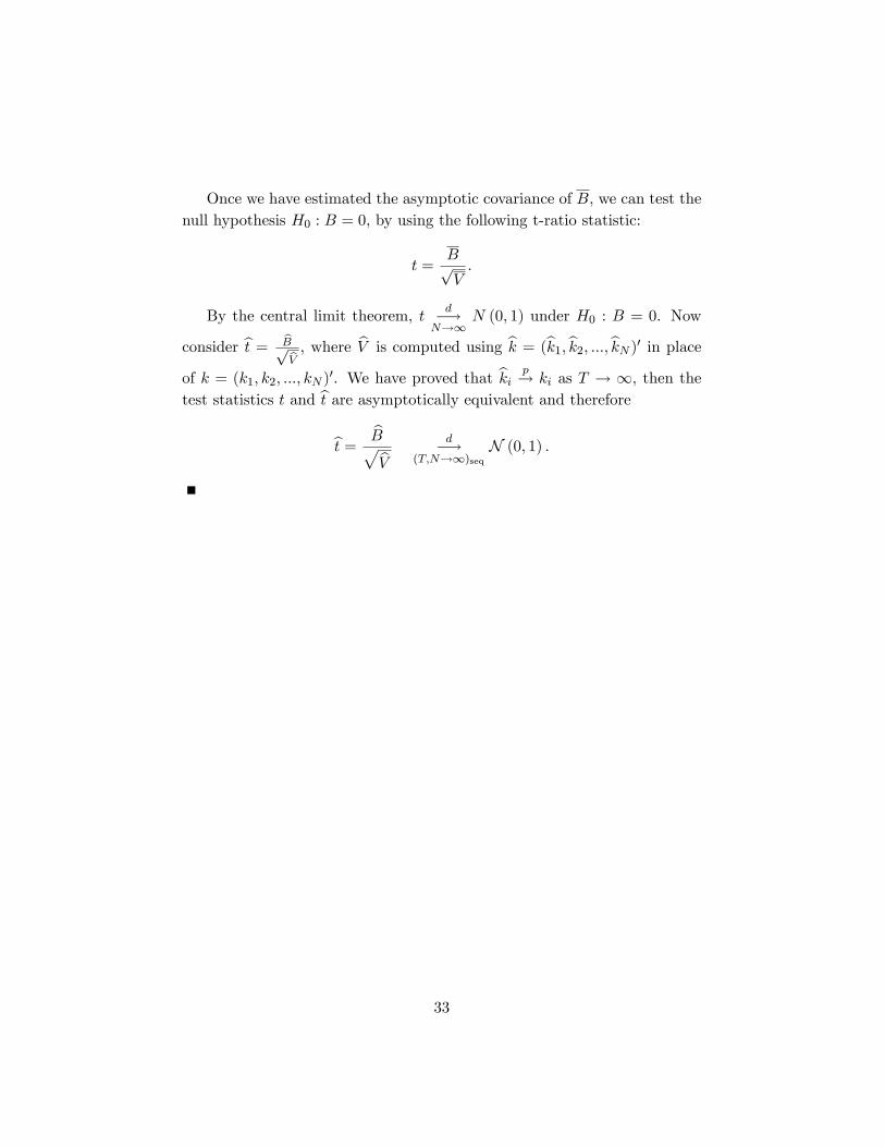
Once we have estimated the asymptotic covariance of B, we can test thenull hypothesis H0 : B = 0, by using the following t-ratio statistic:
t =BpV:
By the central limit theorem, t d�!N!1
N (0; 1) under H0 : B = 0. Now
consider bt = bBpbV , where bV is computed using bk = (bk1;bk2; :::;bkN )0 in placeof k = (k1; k2; :::; kN )
0. We have proved that bki p! ki as T ! 1, then thetest statistics t and bt are asymptotically equivalent and therefore
bt = bBpbV d�!(T;N!1)seq
N (0; 1) :
33
A.2 Tables and Figures
Table 1: Monte-Carlo ResultsR = 50 a = 0; b = 0:5
Bias Distributions MSE DistributionsBCAF Average Weighted BCAF Average Weighted
N = 10
skewness -0.009 0.003 0.004 0.404 0.438 0.632kurtosis 3.043 3.037 3.038 3.221 3.298 3.823mean 0.000 0.391 -0.001 1.561 1.697 1.916� -th= 0:01 quantile -0.590 -0.091 -0.643 0.911 0.989 1.080� -th= 0:25 quantile -0.169 0.252 -0.186 1.337 1.448 1.608� -th= 0:50 quantile -0.001 0.391 -0.001 1.540 1.672 1.872� -th= 0:75 quantile 0.167 0.530 0.184 1.763 1.918 2.179� -th= 0:99 quantile 0.578 0.879 0.641 2.394 2.642 3.138
N = 20
skewness 0.010 -0.013 0.011 0.442 0.444 0.961kurtosis 3.115 3.084 3.138 3.321 3.321 5.011mean 0.000 0.440 -0.002 1.286 1.466 2.128� -th= 0:01 quantile -0.532 -0.001 -0.690 0.754 0.853 1.117� -th= 0:25 quantile -0.153 0.316 -0.195 1.098 1.247 1.723� -th= 0:50 quantile -0.001 0.440 -0.004 1.266 1.444 2.053� -th= 0:75 quantile 0.151 0.565 0.192 1.452 1.659 2.448� -th= 0:99 quantile 0.535 0.876 0.687 1.987 2.275 3.851
N = 40
skewness -0.015 -0.006 -0.016 0.438 0.448 2.852kurtosis 3.147 3.090 3.600 3.324 3.338 22.203mean 0.000 0.465 0.000 1.147 1.351 6.094� -th= 0:01 quantile -0.515 0.050 -1.209 0.673 0.786 2.165� -th= 0:25 quantile -0.145 0.346 -0.315 0.980 1.150 4.021� -th= 0:50 quantile 0.000 0.465 0.002 1.130 1.331 5.337� -th= 0:75 quantile 0.141 0.583 0.312 1.295 1.529 7.243� -th= 0:99 quantile 0.509 0.876 1.209 1.771 2.100 17.669
34

Table 2: Monte-Carlo ResultsR = 50; a = �0:5; b = 0:5Bias Distributions MSE Distributions
BCAF Average Weighted BCAF Average WeightedN = 10
skewness -0.009 0.005 0.004 0.404 0.395 0.632kurtosis 3.043 3.016 3.038 3.221 3.228 3.823mean 0.000 0.000 -0.001 1.561 1.547 1.916� -th= 0:01 quantile -0.590 -0.511 -0.643 0.911 0.905 1.080� -th= 0:25 quantile -0.169 -0.149 -0.186 1.337 1.326 1.608� -th= 0:50 quantile -0.001 0.000 -0.001 1.540 1.526 1.872� -th= 0:75 quantile 0.167 0.147 0.184 1.763 1.745 2.179� -th= 0:99 quantile 0.578 0.516 0.641 2.394 2.369 3.138
N = 20
skewness 0.010 -0.015 0.011 0.442 0.414 0.961kurtosis 3.115 3.071 3.138 3.321 3.283 5.011mean 0.000 0.000 -0.002 1.286 1.272 2.128� -th= 0:01 quantile -0.532 -0.462 -0.690 0.754 0.746 1.117� -th= 0:25 quantile -0.153 -0.130 -0.195 1.098 1.089 1.723� -th= 0:50 quantile -0.001 0.000 -0.004 1.266 1.254 2.053� -th= 0:75 quantile 0.151 0.130 0.192 1.452 1.435 2.448� -th= 0:99 quantile 0.535 0.456 0.687 1.987 1.951 3.851
N = 40
skewness -0.015 -0.005 -0.016 0.438 0.414 2.852kurtosis 3.147 3.090 3.600 3.324 3.266 22.203mean -0.002 0.000 0.000 1.147 1.133 6.094� -th= 0:01 quantile -0.515 -0.426 -1.209 0.673 0.667 2.165� -th= 0:25 quantile -0.145 -0.123 -0.315 0.980 0.971 4.021� -th= 0:50 quantile -0.002 0.000 0.002 1.130 1.116 5.337� -th= 0:75 quantile 0.141 0.121 0.312 1.295 1.278 7.243� -th= 0:99 quantile 0.509 0.424 1.209 1.771 1.733 17.669
35

Table 3: Monte-Carlo ResultsN = 10; R = 500; 1; 000, a = 0; b = 0:5
Bias Distributions MSE DistributionsBCAF Average Weighted BCAF Average Weighted
N = 10, R = 500skewness 0.001 -0.015 -0.002 0.408 0.452 0.408kurtosis 3.058 3.065 3.066 3.308 3.390 3.314mean 0.000 0.391 0.000 1.532 1.697 1.559� -th= 0:01 quantile -0.434 -0.091 -0.437 0.893 0.982 0.913� -th= 0:25 quantile -0.124 0.254 -0.126 1.312 1.448 1.334� -th= 0:50 quantile 0.000 0.391 0.000 1.512 1.672 1.539� -th= 0:75 quantile 0.123 0.529 0.124 1.729 1.918 1.760� -th= 0:99 quantile 0.433 0.870 0.436 2.359 2.645 2.394
Bias Distributions MSE DistributionsBCAF Average Weighted BCAF Average Weighted
N = 10; R = 1; 000
skewness 0.009 0.001 0.011 0.414 0.453 0.413kurtosis 3.064 3.051 3.061 3.300 3.374 3.295mean 0.000 0.392 0.000 1.535 1.695 1.541� -th= 0:01 quantile -0.424 -0.088 -0.424 0.902 0.990 0.909� -th= 0:25 quantile -0.122 0.253 -0.122 1.310 1.447 1.321� -th= 0:50 quantile 0.000 0.392 0.000 1.507 1.670 1.520� -th= 0:75 quantile 0.122 0.531 0.122 1.724 1.916 1.739� -th= 0:99 quantile 0.428 0.876 0.430 2.343 2.635 2.360
36

Table 4: Monte-Carlo ResultsN = 40, R = 2; 000, 4; 000, a = 0; b = 0:5
Bias Distributions MSE DistributionsBCAF Average Weighted BCAF Average Weighted
N = 40, R = 2; 000skewness -0.024 0.006 -0.022 0.407 0.452 0.408kurtosis 3.151 3.139 3.143 3.252 3.330 3.252mean 0.000 0.466 0.000 1.127 1.355 1.149� -th= 0:01 quantile -0.370 0.049 -0.374 0.668 0.786 0.680� -th= 0:25 quantile -0.103 0.348 -0.103 0.965 1.153 0.983� -th= 0:50 quantile 0.000 0.464 0.000 1.121 1.334 1.133� -th= 0:75 quantile 0.103 0.582 0.105 1.271 1.533 1.296� -th= 0:99 quantile 0.363 0.879 0.366 1.728 2.109 1.760
Bias Distributions MSE DistributionsBCAF Average Weighted BCAF Average Weighted
N = 40, R = 4; 000skewness 0.003 0.006 0.002 0.409 0.458 0.415kurtosis 3.132 3.106 3.125 3.255 3.325 3.256mean 0.000 0.465 0.000 1.127 1.355 1.137� -th= 0:01 quantile -0.361 0.053 -0.364 0.666 0.790 0.673� -th= 0:25 quantile -0.103 0.348 -0.103 0.966 1.153 0.975� -th= 0:50 quantile 0.000 0.464 0.000 1.111 1.333 1.122� -th= 0:75 quantile 0.102 0.581 0.103 1.271 1.533 1.283� -th= 0:99 quantile 0.363 0.878 0.364 1.725 2.112 1.739
37

Table 5: The Brazilian Central Bank Focus SurveyComputing Average Bias and Testing the No-Bias Hypothesis
Horizon (h) Avg. Bias bB H0 : B = 0
p-value6 0:06187 0:063
Notes: (1) N = 18, R = 26, P = 15, and h = 6 months ahead.
Table 6: The Brazilian Central Bank Focus SurveyComparing the MSE of Simple Average Forecast with that ofthe Bias-Corrected Average Forecast and the Weighted Average
ForecastForecast Horizon (a) MSE (b) MSE (c) MSE (b)/(a) (c)/(a)
(h) BCAF Average Weighted Avg.Forecast Forecast
6 0:0683 0:0808 0:2665 1:182 3:902
Notes: (1) N = 18, R = 23 and P = 18, and h = 6 months ahead.
38