Embed Size (px)
Citation preview
A numerical studyof an ill-posed Boussinesq equation
arising in water waves and nonlinear lattices:Filtering and regularization techniques 1
Prabir Daripa *, Wei Hua
Texas A&M University, Department of Mathematics, College Station, TX 77843, USA
Abstract
We consider an ill-posed Boussinesq equation which arises in shallow water waves
and nonlinear lattices. This equation has growing and decaying modes in the linear as
well as nonlinear regimes and its linearized growth rate r for short-waves of wave-
number k is given by r � k2. Previous numerical studies have addressed numerical
di�culties and construction of approximate solutions for ill-posed problems with short-
wave instability up to r � k, e.g. Kelvin±Helmholtz �r � k� and Rayleigh±Taylor �r ����kp � instabilities. These same issues are addressed and critically examined here for the
present problem which has more severe short-wave instability. In order to develop
numerical techniques for constructing good approximate solutions of this equation, we
use a ®nite di�erence scheme to investigate the e�ect of this short-wave instability on the
numerical accuracy of the exact solitary wave solution of this equation. Computational
evidence is presented which indicates that numerical accuracy of the solutions is lost
very quickly due to severe growth of numerical errors, roundo� as well as truncation.
We use both ®ltering and regularization techniques to control growth of these errors
and to provide better approximate solutions of this equation. In the ®ltering technique,
numerical experiments with three types of spectral ®lters of increasing order of regu-
larity are performed. We examine the role of regularity of these ®lters on the accuracy of
the numerical solutions. Numerical evidence is provided which indicates that the reg-
ularity of a ®lter plays an important role in improving the accuracy of the solutions. In
the regularization technique, the ill-posed equation is regularized by adding a higher
Applied Mathematics and Computation 101 (1999) 159±207
* Corresponding author.1 This research was supported by NSF grants No. DMS±9208061 and by the O�ce of the Vice
President for Research and Associate Provost for Graduate Studies at Texas A&M University.
0096-3003/99/$ ± see front matter Ó 1999 Elsevier Science Inc. All rights reserved.
PII: S0 0 96 -3 0 03 (9 8 )1 00 7 0- X

order term to the equation. Two types of higher order terms are discussed: (i) one that
diminishes the growth rate of all modes below a cuto� wavenumber and sets the growth
rate of all modes above it to zero; and (ii) the other one diminishes the growth rate of all
modes and the growth rate asymptotically approaches to zero as the wavenumber ap-
proaches in®nity. We have argued in favor of the ®rst type of regularization and nu-
merical results using a ®nite di�erence scheme are presented. Numerical evidence is
provided which suggests that regularization in combination with the most regular (C2
here) spectral ®lter for small values of the regularization parameter can provide good
approximate solutions of the ill-posed Boussinesq equation for longer time than possible
otherwise. Some of the ideas presented here can possibly be utilized for solving other ill-
posed problems with severe short-wave instabilities and may have an important role to
play in numerical studies of their solutions. Ó 1999 Elsevier Science Inc. All rights
reserved.
Keywords: Ill-posed problem; Boussinesq equation; Solitary wave; Water waves; Finite di�erence
equation
1. Introduction
In this paper, we are interested in the numerical study of the ill-posedBoussinesq equation
utt � �p�u��xx � uxxxx; �1:1�with p�u� � u� u2 and subject to some restricted class of initial data, u�x; 0�and ut�x; 0� to be discussed later. The corresponding linearized PDE has de-caying as well as growing modes, ert�ikx, with the dispersion relation about aconstant state, uc, given by
r� � �k����������������������k2 ÿ p0�uc�
p: �1:2�
Without any loss of generality, we have used waves with wavelength 2p in thedispersion relations. (Thus, the wavenumber k in Eq. (1.2) actually refers to�2p=L�k whenever this problem is considered in a domain of length L.) Theequilibrium states in the elliptic region (i.e. p0�uc� � 1� 2uc < 0� are unstableto all modes and the states in the hyperbolic region are unstable to modesjkj > ������������
p0�uc�p
. Since the growth rate, i.e. the real part of r�, is a monotonicallyincreasing function of the wavenumber, there is no wavenumber with maximalrate of stability. According to the dispersion relation (1.2) short-wave insta-bility is given by
r � k2 as k !1: �1:3�It should be noted that the well-posed Boussinesq equation di�ers from
Eq. (1.1) only in the sign of the term containing uxxxx. The well-posed equationis easy to solve numerically [9] and does not concern us in this paper. More-
160 P. Daripa, W. Hua / Appl. Math. Comput. 101 (1999) 159±207
over, we are interested only in the hyperbolic regime of this equation and thuswe are not interested in this paper numerical issues in the subcritical (i.e.p0�uc� � 1� 2uc < 0� or critical regimes (i.e. p0�uc� � 1� 2uc � 0�.
Di�culty in solving the ill-posed equation (1.1), analytically and numeri-cally, arises due to severe short-wave instability (1.3). In general, classical so-lutions of this equation with arbitrary initial data are not expected to exist forpositive time except for some special choices of initial data. Using inversescattering technique, Deift et al. [4] have implicitly constructed solutions ofEq. (1.1) without the term uxx, some global and some that blow up in ®nitetime. (The term uxx in Eq. (1.1) can be removed by replacing u by uÿ 1
2.) Except
for arbitrary constants, only other C1 solutions known to exist for thisequation are of soliton-type (singlet as well as doublet) [5,10]. The solitarywave solution is given by [5,10]
us�x; t� � A sech2��������A=6
p�xÿ ct � x0�
n o� bÿ 1
2
� �; �1:4�
where A is the amplitude of the solitary wave, b is a free parameter and c �� �����������������������
2�b� A=3�pis the speed of the solitary wave. Solitary wave corresponding
to b � 12
and x0 � 0 which are convenient for numerical purposes in this paperis given by
us�x; t� � A sech2��������A=6
p�xÿ ct�
n o: �1:5�
The ill-posed Boussinesq equation (1.1) commonly describes propagation ofsmall amplitude long waves (long compared to the amplitude of the wave) inseveral physical contexts including shallow water under gravity [16] and onedimensional nonlinear lattices [17]. Asymptotic expansion of appropriatephysical equations in some small parameter in k usually gives rise to the ill-posed Boussinesq equation within some order of approximation. For example,in Appendix A we describe brie¯y from Ref. [16] the origin of this equation inthe context of shallow water waves. Usually, as in the case of water waves, thisequation is physically relevant only for small k and breaks down for large k.Therefore severe growth rate of waves with large k may not appear to be animportant issue. However, these short-waves will enter into the calculation dueto numerical error as well as due to nonlinearity of the equation. Thereforeaccurate computation of even physically relevant solutions of this equation isnot possible without circumventing numerical di�culties due to this short-waveinstability. The truncation and roundo� errors during machine computationsintroduce spurious perturbations at all scales, small and large. These smallscale perturbations which grow very rapidly cause signi®cant di�culty inconstructing good approximate solutions of this equation. Such di�culties alsooccur for other ill-posed problems such as Kelvin±Helmholtz instability [7] andRayleigh±Taylor instability [2]. However, short-wave instabilities are less
P. Daripa, W. Hua / Appl. Math. Comput. 101 (1999) 159±207 161

severe for these �r � ���kp
for Kelvin±Helmholtz and r � k for Rayleigh±Tay-lor) cases. Therefore it is somewhat more challenging and interesting to assesthe level of numerical di�culties that this severe short-wave instabilities pose.Our aim in this paper is to explore ways to circumvent these di�culties in orderto obtain good approximate solutions of this equation subject to appropriateinitial data. Hope is that this will allow further numerical studies of this andother severely ill-posed equations and their solutions.
It may be worth mentioning here that, in the weakly nonlinear limit, shallowwater wave equation (A.7) for long waves (see Appendix A) reduces to the wellknown Korteweg±de Vries (KdV) equation [16]
ut � uux � uxxx � 0: �1:6�The di�erence between this equation and the Boussinesq equation is that thelatter allows bidirectional waves while KdV only unidirectional waves.
At this point we would like to mention a loose analogy between Boussinesqequations (ill-posed as well as well-posed) and isothermal equations of¯uid ¯ows [12,13]. The Boussinesq equation (1.1) can be viewed as a degeneratecase of the following 2� 2 system of ®rst order equations with � � 0 andd � ÿ1,
ut ÿ vx � 0; vt ÿ �p�u��x � duxxx � �vxx: �1:7�This system describes isothermal ¯uid ¯ows with speci®c volume u, velocity v,pressure law p�u�, viscosity coe�cient � and capillary coe�cient d [12,13].Therefore, Boussinesq equations also describe the isothermal inviscid ¯uid ¯owin one dimension with quadratic pressure law and a capillarity coe�cient whichis positive for the well-posed Boussinesq equation �d � 1� and negative for theill-posed Boussinesq equation �d � ÿ1�. The ill-posedness of Eq. (1.1) can beviewed as a result of this negative capillarity. It should not be confused with thesurface tension e�ect in the context of water waves. As discussed before and inAppendix A, the ill-posed Boussinesq equation arises out of asymptotic ex-pansion of shallow water equations which contain no surface tension e�ect (seealso [16]). The system (1.7) with positive capillary coe�cient and various cubicpressure laws including van der Waals pressure law has been studied as modelsof dynamic phase transition by A�ouf and Ca¯isch [1] and Slemrod [12,13]among others. The hyperbolic region of the quadratic pressure law of theBoussinesq system has the same qualitative feature as the van der Waalspressure law at high enough temperature. It appears that the Boussinesq sys-tem due to its exact soliton-type solutions and simplicity may be useful innumerical study of conservation laws of mixed type.
The ill-posed Boussinesq equation (1.1) which arises in various contexts asdiscussed above may not always have a sound physical basis for explainingphenomena at small scales. However, we believe that mathematical and com-
162 P. Daripa, W. Hua / Appl. Math. Comput. 101 (1999) 159±207
putational di�culties associated with the study of this equation can be moregeneric than it appears to be and may occur in other physical and mathematicalcontexts. Moreover, numerical methods which will allow construction of goodapproximate solutions of such severely ill-posed problems are not known andare not easy to construct without proper understanding of the e�ect of suchshort-wave instability on the accuracy of the numerical solutions. The Bous-sinesq equation (1.1) provides a simple case of severely ill-posed nonlinearproblems which also has exact traveling wave solutions. These exact solutionscan be used during machine computations to develop appropriate numericalmethods that can be useful not only for solving this equation but possibly otherill-posed problems as well. Numerical experiments can then possibly be per-formed with these numerical methods to investigate further the mathematicalproperties of this and other similar imposed problems.
The paper is laid out as follows. In Section 2 we present a ®nite di�erencescheme which is second order accurate in time and space. We present a line-arized stability analysis of this scheme and derive its dispersion relation. Meshsizes based on good approximation of the analytical dispersion relation by thenumerical one are obtained. These mesh sizes are then used in single anddouble precision calculation and results are presented to show the dangerouse�ect of machine roundo� error on the accuracy of numerical solutions. Wecompute error estimates of the numerical solutions to provide numerical evi-dence of convergence of the numerical schemes. In Section 3, we apply thenumerical scheme with three ®lters of increasing order of regulatory to showthat the spurious errors introduced by ®nite digit arithmetics of machinecomputation can be controlled to a considerable extent by appropriate choiceof ®lters. We present a new ®lter which is twice continuously di�erentiable andpresent in detail application procedure of this ®lter. Numerical results with this®lter are presented to justify its usefulness in the numerical construction ofapproximate solutions of ill-posed problems. In Section 4, we present viscosity-like and surface-tension like regularization techniques by adding higher orderterms to Eq. (1.1). We carry out their linearized stability analysis and derivetheir dispersion relations. There we argue based on linearized stability analysisand physical consideration that surface-tension-like regularization is moreappropriate and is likely to give better approximate solution. Moreover, it iseasier to implement surface-tension-like regularization than the viscosity-likeregularization. The numerical scheme of Section 2 is then extended for theregularized equation with surface-tension-like regularization. Linearized sta-bility analysis of this scheme is carried out and numerical results with thisscheme are presented. We ®nd that these numerical solutions for modest valuesof regularizing parameters can also provide very good approximations to so-lutions of the ill-posed Boussinesq equation (1.1). In Section 5, we summarizeand discuss our ®ndings and mention some problems which are areas of futureresearch.
P. Daripa, W. Hua / Appl. Math. Comput. 101 (1999) 159±207 163
2. Numerical scheme
2.1. Finite di�erence scheme
Eq. (1.1) is solved numerically in a ®nite domain, a6 x6 b, for t > 0. We use®nite di�erence method with uniform grid spacings h in x and s in t. Using vn
j todenote the approximate value of u�x; t� at x � a� jh; t � ns and using usual®nite di�erence operators D� and Dÿ to denote forward and backward dif-ferences, Eq. (1.1) can be approximated by the Finite Di�erence Equation(FDE).
D�t Dÿt vnj
s2� D�x Dÿx �p�vn
j ��h2
� �D�x Dÿx �2�vn�1
j � vnÿ1j �
2h4; �2:1�
for s > 0 and 0 < j < N�06 j < N in case of periodic domain) wherebÿ a � Nh. The truncation error is E�h; s� � O�h2� �O�s2�.
Following A�ouf and Ca¯isch [1], we use the following fourth order accu-rate boundary conditions to estimate boundary conditions v�aÿ h; ns� andv�b� h; ns�, for n P 0.
v�aÿ h; ns� � ÿ 3
2v�a; ns� � 3v�a� h; ns� ÿ 1
2v�a� 2h; ns� ÿ 3v0�a; ns�h;
�2:2�
v�b� h; ns� � ÿ 3
2v�b; ns� � 3v�bÿ h; ns� ÿ 1
2v�bÿ 2h; ns� � 3v0�b; ns�h
�2:3�and the following third order accurate initialization to estimatev�jh; s�; 06 j6N
v�:; s� � v�:; 0� � v0�:; 0�s� v00�:; 0� s2
2�O�s3�; �2:4�
where v�:; s� and v0�:; s� are given, and v00�:; s� can be obtained directly fromusing the Boussinesq equation (1.1).
We computed numerical solutions in the interval �a; b� witha � ÿ128; b � 128, subject to the following initial conditions
u�x; 0� � us�x; 0�; ut�x; 0� � ust �x; 0� �2:5�
and the boundary conditions
u�a; t� � us�a; t�; u�b; t� � us�b; t�; t > 0; �2:6�where us�x; t� is given by (1.5). The computations were performed in single (7digit arithmetic) and double (15 digit arithmetic) precisions. Below we often usethe notations `sp' for `single precision' and `dp' for `double precision'.
164 P. Daripa, W. Hua / Appl. Math. Comput. 101 (1999) 159±207
Our choice of the computational domain �ÿ128; 128� allows the physicalboundaries to be well-away from the support of the solitary wave so that ap-proximate numerical solutions remain almost periodic within machine preci-sion. The lack of periodicity of the numerical solutions or/and theinappropriateness of the use of Fourier ®ltering are not relevant issues duringthe relatively short time intervals of computation that are involved here. This,in a way, is very convenient as it allows us to focus solely on the numericaldi�culties associated with the severe short wave instability of this problem.The numerical results that are reported in this paper involve time intervalduring which the movement of the solitary wave is so small compared to thecomputational interval that the approximate numerical solutions reported hereremain periodic within an error of the size of the machine precision. ThereforeFourier ®ltering that we use in Section 3 remains appropriate for all ourcomputations in this paper.
2.2. Linearized stability of the FDE about any constant state uc.
Any constant state, u � uc, is a solution to both the PDE and the FDE.Denoting the perturbation about the constant state, uc, by ~vn
j , and then lin-earizing the FDE about this constant state we obtain
D�t Dÿt ~vnj
s2� �p0�uc��
D�x Dÿx ~vnj
h2� �D
�x Dÿx �2�~vn�1
j � ~vnÿ1j �
2h4: �2:7�
With ~vnj � qneinj in Eq. (2.7) (where q � ebs, n � kh; k is the wavenumber and
real part of b is the growth rate), the dispersion relation for the numericalscheme is
1ÿ 8r2 sin4 n2
� �q2 � 2 2k2p0�uc� sin2 n
2ÿ 1
� �q� 1ÿ 8r2 sin4 n
2
� �� 0;
�2:8�where r � s=h2 and k � s=h.
The dispersion relations (1.2) for the linearized Boussinesq equation andEq. (2.8) for the linearized FDE are qualitatively similar in the sense that thereare neutral, growing and decaying modes in both the FDE and the PDE if uc, hand s satisfy the following relations:
k26 1
p0�uc� and r <1
2���2p : �2:9�
The ®rst of these conditions is the usual CFL condition which ensures thatthe numerical scheme has only decaying modes in the absence of uxxxx term inEq. (1.1). This is consistent with the corresponding exact dispersion relation,i.e. Eq. (1.2) without the k2 term. The second of these condition is slightlystringent than the usual stability condition, r < 1
2, associated with the numerical
P. Daripa, W. Hua / Appl. Math. Comput. 101 (1999) 159±207 165
scheme for the parabolic heat equation. Eq. (1.1) without the hyperbolic termis a higher order parabolic equation than the heat equation and it has stable aswell as unstable modes (see Eq. (1.2)). The condition r < 1
2ensures that our
numerical scheme without the hyperbolic term will also have stable and un-stable modes. Modes with in®nite growth/decay rate are allowed by the re-quirement r < 1
2. We prefer to avoid these modes. This is accomplished by
making this criterion more stringent as in Eq. (2.9). For our later numericalpurposes it is convenient to rewrite Eq. (2.9) in terms of s and h.
h6 2���2p������������
p0�uc�p and
sh2<
1
2���2p : �2:10�
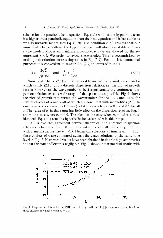
Numerical scheme (2.1) should preferably use values of grid sizes s and hwhich satisfy (2.10) allow discrete dispersion relation, i.e. the plot of growthrate ln jqj=s versus the wavenumber k, best approximate the continuous dis-persion relation over as wide range of the spectrum as possible. Fig. 1 showsthe plot of growth rate versus the wavenumber for the PDE and FDE forseveral choices of h and s all of which are consistent with inequalities (2.9). Inour numerical experiments below u�x� takes values between 0.0 and 0.5 for allx. The value of uc in this range has little e�ect on the dispersion relation. Fig. 1shows the case when uc � 0:0. The plot for the case when uc � 0:5 is almostidentical. Eq. (1.1) remains hyperbolic for values of u in this range.
Fig. 1 shows that agreement between theoretical and numerical dispersionrelations is better with s � 0:085 than with much smaller time step s � 0:01with a mesh spacing size h � 0:5. Numerical solutions at time level t � 1 forthese choices of s are compared against the exact solutions at the same timelevel in Fig. 2. Numerical results have been obtained in double digit arithmeticsso that the roundo� error is negligible. Fig. 2 shows that numerical results with
Fig. 1. Dispersion relation for the PDE and FDE: growth rate ln jqj=s versus wavenumber k for
three choices of h and s when uc � 0:0.
166 P. Daripa, W. Hua / Appl. Math. Comput. 101 (1999) 159±207
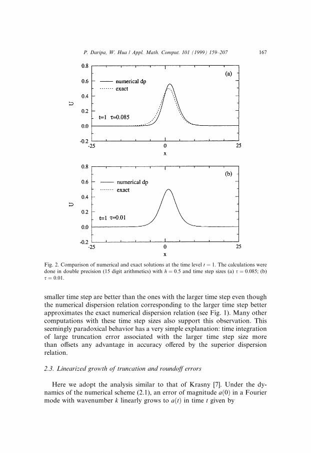
smaller time step are better than the ones with the larger time step even thoughthe numerical dispersion relation corresponding to the larger time step betterapproximates the exact numerical dispersion relation (see Fig. 1). Many othercomputations with these time step sizes also support this observation. Thisseemingly paradoxical behavior has a very simple explanation: time integrationof large truncation error associated with the larger time step size morethan o�sets any advantage in accuracy o�ered by the superior dispersionrelation.
2.3. Linearized growth of truncation and roundo� errors
Here we adopt the analysis similar to that of Krasny [7]. Under the dy-namics of the numerical scheme (2.1), an error of magnitude a�0� in a Fouriermode with wavenumber k linearly grows to a�t� in time t given by
Fig. 2. Comparison of numerical and exact solutions at the time level t � 1. The calculations were
done in double precision (15 digit arithmetics) with h � 0:5 and time step sizes (a) s � 0:085; (b)
s � 0:01.
P. Daripa, W. Hua / Appl. Math. Comput. 101 (1999) 159±207 167
t � 1
x�t� lna�t�a�0� ; �2:11�
where x�t� is the linearized growth rate of the Fourier mode. For appropriatechoices of h and s, the numerical dispersion relation can be approximated by
x�k� � c�k�k2; �2:12�where c�k� is some function of k. For c�k� � 1 as k !1, we have the linearizeddispersion relation of the PDE in this limit. If a�0� � 10ÿd and a�t1� � 10ÿp forthe fastest growing Fourier mode in the numerical scheme, then it follows fromEq. (2.11) and Eq. (2.12) that
t1 � hp
� �2
�d ÿ p� ln 10; �2:13�
where we have used k � O�N=2�, the wavenumber of fastest growing modeparticipating in the numerical scheme with N number of grid points, and c�k� �1 due to moderately good agreement between numerical and exact dispersionrelations for certain choices of h and s in Fig. 1. Similar arguments would givet1 � O�h� for KH (see also [7]), and t1 � O� ���hp � for RT types of instabilities.The arguments leading up to Eq. (2.13) here is similar to that used by Krasny[7] for KH instability.
Eq. (2.13) shows that errors in the high wavenumber mode grow more rap-idly with decreasing mesh sizes. Such severe growth or error in the high wavenumber modal amplitudes can cause signi®cant loss of numerical accuracy inthe computed solutions as seen in Fig. 3. For example, an initial error ofmagnitude 10ÿ7 (such errors are likely in single precision calculation) will in-crease to a value of 10ÿ5:5 in a single time step when s � 0:085 and h � 0:5, theparameter values corresponding to numerical dispersion relation that best ap-proximates the exact dispersion relation (see Fig. 1). In reality, this error can beeven larger due to nonlinear ill-posedness of the Boussinesq equation. Such anampli®cation of machine roundo� error in a single time step can cause seriousdi�culties in advancing the solutions correctly any further. Therefore the timestep sizes must be chosen smaller than this so that postprocessing of data aftereach or few time steps will make it possible to reduce the spurious e�ects ofroundo� error. A smaller choice of s, of course, entails a tradeo� between theerror in the numerical solution due to disagreement between numerical andtheoretical dispersion relations and the error in the numerical solution due tocatastrophic growth of spurious errors in a single time step. Below we exemplifyin some detail the numerical di�culties due to short-wave instabilities.
The results in Fig. 3 shows the e�ect of roundo� error on the numericalaccuracy of the solution (here the e�ect of truncation error on the solution iskept negligibly small by integrating the solution for short time). Fig. 3(a) and3(b) show numerical and exact solutions at the time level t � 1 with mesh sizesh � 1 and h � 0:5 respectively. Numerical computations have been performed
168 P. Daripa, W. Hua / Appl. Math. Comput. 101 (1999) 159±207

in single precision. We see in these plots that very accurate solutions are ob-tained with h � 1:0 suggesting that the e�ect of truncation error on the solutionat t � 1 is small. The e�ect of truncation error on the numerical solution at t �1 is even smaller with smaller time step size h � 0:5 in Fig. 3(b). However, these®gures show that numerical solutions get even worse with small time step sizeh � 0:5 even though the truncation error is smaller. Smaller mesh size herecauses participation of higher wavenumber modes. Short-wave instabilitycauses rapid growth of spurious perturbations in these mode introduced byroundo� errors resulting in severe deterioration of numerical solutions as seenin this ®gure. In general, any gain in the accuracy of numerical solutions due tosmaller mesh sizes is quickly lost due to these instabilities. This brings com-putations to a halt sooner or later depending on the mesh size and the machineprecision used.
The truncation error can cause signi®cant loss in the accuracy of numericalsolutions when calculations are carried out for longer time. For example,
Fig. 3. Comparison of numerical and exact solutions at the time level t � 1. The calculations were
done in single precision (7 digit arithmetics) with di�erent mesh size (a) h � 1; (b) h � 0:5.
P. Daripa, W. Hua / Appl. Math. Comput. 101 (1999) 159±207 169

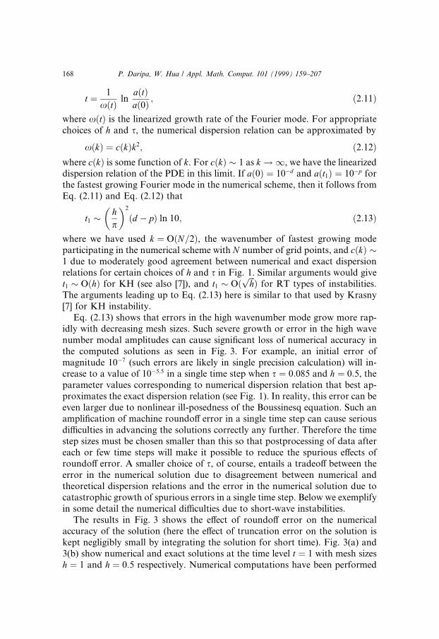
advancing the numerical solution in Fig. 3(a) further deteriorates the accuracyof the numerical solution in Fig. 4(a) and higher machine precision calculationdoes not improve the solution either as seen in Fig. 4(b). In fact, numericalsolutions obtained in single (Fig. 4(a)) and double (Fig. 4(b)) precision cal-culations appear to be almost the same. This is due to the fact that the dete-riorating e�ect of roundo� error on the accuracy of numerical solutions insingle precision calculation is almost negligible compared to that of the trun-cation error. Also notice in Fig. 4(c) that all Fourier modes participating in thecalculations here have amplitudes greater than the roundo� error of singleprecision calculation.
Above example does not show that calculations on a higher precision ma-chine can improve the accuracy of numerical solutions. This is due to the factthat roundo� error is not the cause of inaccuracies in numerical solution at t �3:5 in Fig. 4.
The inaccuracies in the numerical solution shown in Fig. 3(b) is due toroundo� error as discussed earlier and can be considerably improved withhigher precision calculation as seen in Fig. 5(a) and 5(b). Fig. 5(a) and 5(b)compare numerical solutions obtained in single and double precisions respec-tively with mesh size h � 0:5. Fig. 5(c) shows that all participating modes haveamplitudes greater than roundo� error of double precision (15 digit arithme-tics) calculations and approximately half of these participating modes withhigh wavenumber have amplitudes less than the roundo� error of single pre-cision (7 digit arithmetics) calculations. Therefore, initial amplitudes of thesehigh wavenumber modes are severely contaminated with spurious perturba-tions introduced by machine roundo� error in single precision calculations.Such contamination is relatively much less in double precision calculation as isevident from Fig. 5(c).
In summary, Figs. 3±5 show that numerical construction of good approxi-mate numerical solutions for long time requires proper control of truncation aswell as roundo� errors. We have seen and argued above that as we keep re-®ning the mesh size, truncation error becomes less of a problem and roundo�error becomes more of a serious problem to the construction of a good ap-proximate solution. In other words, growth rate of short waves restricts theaccuracy of numerical solutions that can be obtained from ®nite precisionmachine calculations. Unless the data are perturbed so as to suppress thespurious e�ects of roundo� error or the dispersion relation is modi®ed in aclever way, computation of good approximations to long-time solutions isdi�cult. According to Tikhonov and Arsenin [14], the ®rst of these methods isknown as ®ltering method and the second of these methods is known as reg-ularization method. Before we discuss, implement and show the performanceof these methods in the Sections 3 and 4, we provide numerical evidence ofconvergence of the numerical scheme (2.1) in the following section.
170 P. Daripa, W. Hua / Appl. Math. Comput. 101 (1999) 159±207
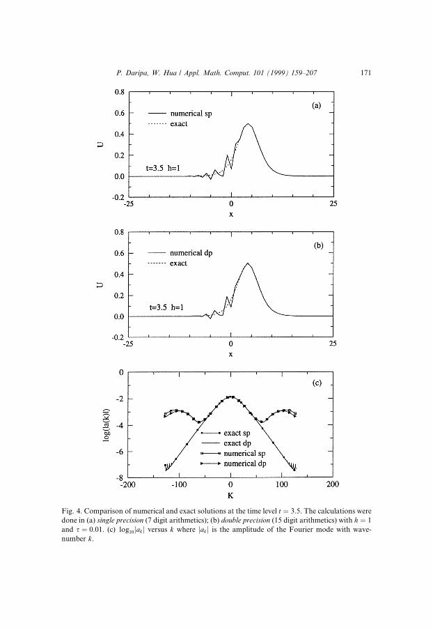
Fig. 4. Comparison of numerical and exact solutions at the time level t � 3:5. The calculations were
done in (a) single precision (7 digit arithmetics); (b) double precision (15 digit arithmetics) with h � 1
and s � 0:01. (c) log10jak j versus k where jak j is the amplitude of the Fourier mode with wave-
number k.
P. Daripa, W. Hua / Appl. Math. Comput. 101 (1999) 159±207 171
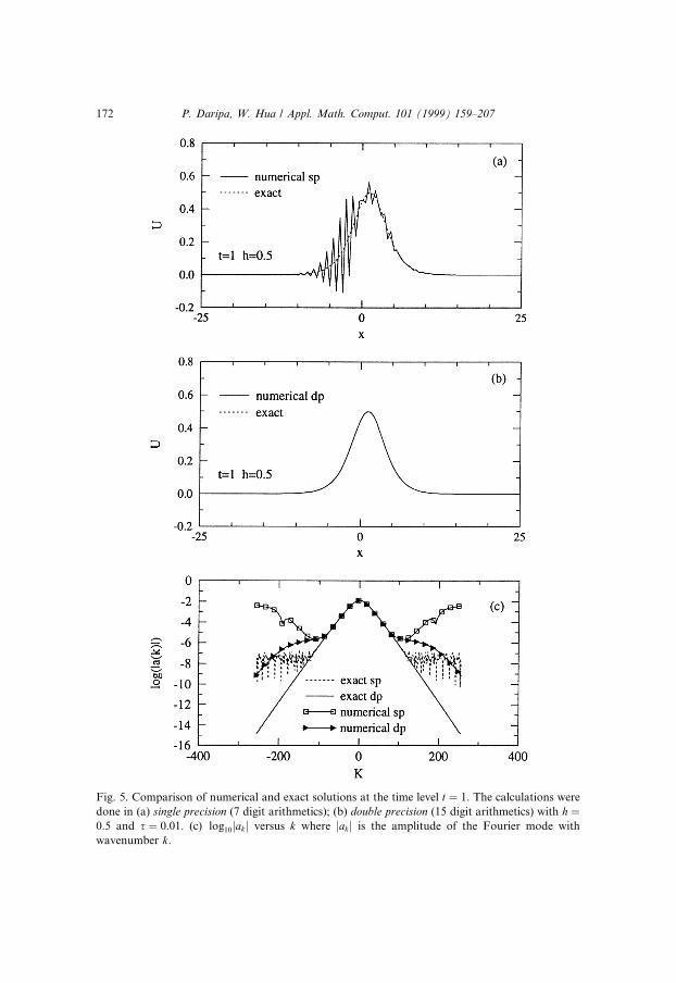
Fig. 5. Comparison of numerical and exact solutions at the time level t � 1. The calculations were
done in (a) single precision (7 digit arithmetics); (b) double precision (15 digit arithmetics) with h �0:5 and s � 0:01: (c) log10jak j versus k where jak j is the amplitude of the Fourier mode with
wavenumber k.
172 P. Daripa, W. Hua / Appl. Math. Comput. 101 (1999) 159±207
2.4. Numerical evidence of convergence of the numerical scheme (2.1)
A consequence of the short-wave instability of the numerical scheme (2.1) isthat the scheme is linearly unstable. Linearly unstable numerical methods fornon-linear ill-posed problems may, however, converge. For example pointvortex method for the vortex sheet problem, even though unstable, convergesup to the time of singularity formation (see [6]). Therefore it makes sense toinvestigate whether the scheme (2.1) converges or not so that we have somecon®dence in the numerical results presented in this work.
We have seen that spurious error introduced by machine roundo� errorincreases with decreasing mesh size. Therefore, it is di�cult to numericallyinvestigate whether the numerical scheme converges or not under mush re-®nement unless we either ®nd a way to completely eliminate the roundo� erroror study the convergence issues up to a mesh size which is large enough not tocause any signi®cant roundo� error and then extrapolate the behavior of theerror in the limit of zero mesh size. The ®rst method, i.e. complete eliminationof roundo� error regardless of the mesh size, is not practical when computa-tions are carried out on ®nite precision machines and/or algorithms. The sec-ond method involves studying the error in the numerical solution as a functionof mesh size until mesh size is small enough to cause severe growth of spuriousperturbations introduced by roundo� error. Therefore right at the outset wemust emphasize the experimental nature of this investigation. One can at bestdraw inferences from numerical data whether the scheme converges or notfrom this study. Even though this is not a rigorous proof of convergence of thenumerical scheme, we believe that it is worth presenting the results of such anumerical study of the convergence issue.
Numerical estimates of L2 and L1 errors obtained in single and doubleprecision computations are shown in Tables 1 and 2. Table 1 shows these errorsonly up to t � 0:8 because inaccuracies in the numerical solutions due to short-wave instabilities seem to be insigni®cant up to t � 0:8 at which time this errorstarts a�ecting the accuracy of the numerical solutions. In fact, some deterio-ration in the convergence is already evident in this table at t � 0:4; 0:6; 0:8when h � 0:5, indicating the spurious e�ects of short-wave instabilities ratherthan failure of convergence of the numerical scheme. This is borne out by thevalues of these error estimates in Table 2 where calculations are done in doubleprecision. The deteriorating e�ects of the severe short-wave instabilities on theconvergence properties is now felt only at t � 0:8 when h � 0:5 as seen in thistable. Even though accurate computations can be carried out for longer time, wehave shown these estimates up to the same time level as that in Table 1 formaking a relative comparison of accuracies between single and double precisioncalculations. We believe there is enough evidence here which lead us to con-jecture that scheme (2.1) converges for, at least, some ®nite time.
P. Daripa, W. Hua / Appl. Math. Comput. 101 (1999) 159±207 173
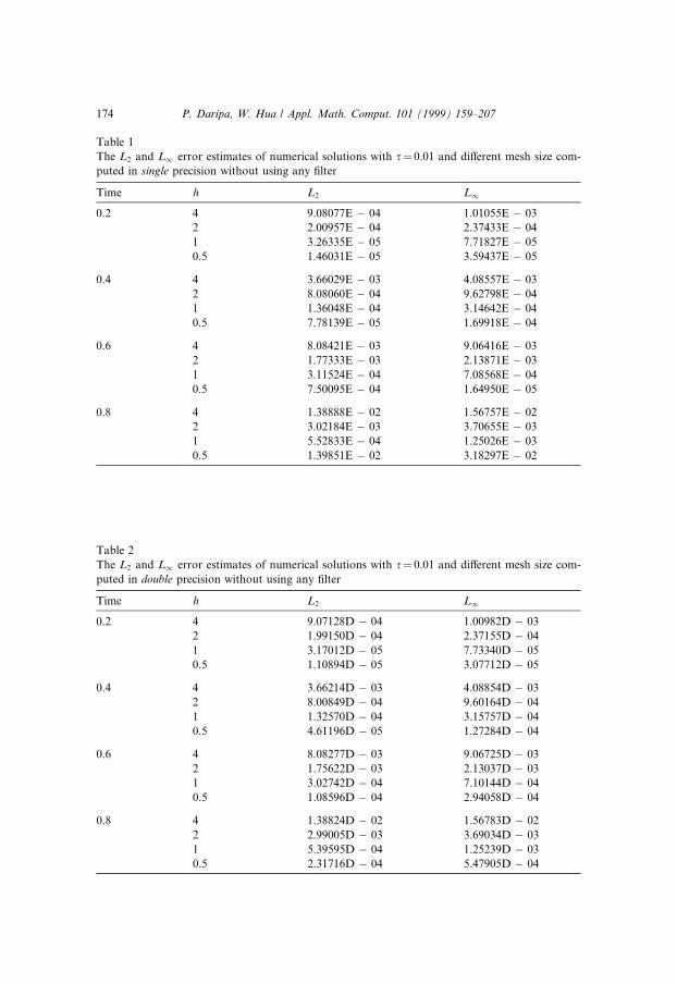
Table 2
The L2 and L1 error estimates of numerical solutions with s� 0.01 and di�erent mesh size com-
puted in double precision without using any ®lter
Time h L2 L1
0.2 4 9.07128D ÿ 04 1.00982D ÿ 03
2 1.99150D ÿ 04 2.37155D ÿ 04
1 3.17012D ÿ 05 7.73340D ÿ 05
0.5 1.10894D ÿ 05 3.07712D ÿ 05
0.4 4 3.66214D ÿ 03 4.08854D ÿ 03
2 8.00849D ÿ 04 9.60164D ÿ 04
1 1.32570D ÿ 04 3.15757D ÿ 04
0.5 4.61196D ÿ 05 1.27284D ÿ 04
0.6 4 8.08277D ÿ 03 9.06725D ÿ 03
2 1.75622D ÿ 03 2.13037D ÿ 03
1 3.02742D ÿ 04 7.10144D ÿ 04
0.5 1.08596D ÿ 04 2.94058D ÿ 04
0.8 4 1.38824D ÿ 02 1.56783D ÿ 02
2 2.99005D ÿ 03 3.69034D ÿ 03
1 5.39595D ÿ 04 1.25239D ÿ 03
0.5 2.31716D ÿ 04 5.47905D ÿ 04
Table 1
The L2 and L1 error estimates of numerical solutions with s� 0.01 and di�erent mesh size com-
puted in single precision without using any ®lter
Time h L2 L1
0.2 4 9.08077E ÿ 04 1.01055E ÿ 03
2 2.00957E ÿ 04 2.37433E ÿ 04
1 3.26335E ÿ 05 7.71827E ÿ 05
0.5 1.46031E ÿ 05 3.59437E ÿ 05
0.4 4 3.66029E ÿ 03 4.08557E ÿ 03
2 8.08060E ÿ 04 9.62798E ÿ 04
1 1.36048E ÿ 04 3.14642E ÿ 04
0.5 7.78139E ÿ 05 1.69918E ÿ 04
0.6 4 8.08421E ÿ 03 9.06416E ÿ 03
2 1.77333E ÿ 03 2.13871E ÿ 03
1 3.11524E ÿ 04 7.08568E ÿ 04
0.5 7.50095E ÿ 04 1.64950E ÿ 05
0.8 4 1.38888E ÿ 02 1.56757E ÿ 02
2 3.02184E ÿ 03 3.70655E ÿ 03
1 5.52833E ÿ 04 1.25026E ÿ 03
0.5 1.39851E ÿ 02 3.18297E ÿ 02
174 P. Daripa, W. Hua / Appl. Math. Comput. 101 (1999) 159±207

3. The ®ltering method
According to Tikhonov and Arsenin [14], the ®ltering method of con-structing approximate solution of ill-posed evolution problems involves se-lective perturbation of the initial data so that a good approximate solution canbe obtained. The choice of correct amount of perturbation is nontrivial andusually depends on the type of problem and the method used to solve theproblem. Since one of the causes of the poor numerical solution here is thegrowth of spurious perturbations introduced by machine roundo� error, per-turbations of the numerical data at various discrete time steps will be chosenhere so as to suppress and possibly eliminate the growth of spurious pertur-bations.
We perturb the data using spectral ®lters in the following way. The ampli-tude of nth Fourier mode of a numerical solution before and after the use of a®lter U�n� are denoted by an and ~an respectively where
~an � anU�n�: �3:1�Two conventional spectral ®lters, U1�n� and U2�n�, that we have used in ad-dition to one more to be constructed and discussed later are>
U1�n� �an ÿ bn
an; n6 nc;
0; n > nc
(�3:2�
and
U2�n� �janj2 ÿ jbnj2janj2
; n6 nc;
0; n > nc:
8<: �3:3�
The cuto� point nc is the smallest wavenumber with amplitude anc� 10ÿm
where m is the computational noise level and is determined by the machinerepresentation of initial condition's Fourier spectrum. Below, we call `m' the®lter level or `¯' in short. Thus ¯� 5 below means that nc is such that anc
�10ÿ5: We have performed numerical experiments with various ®lter levels eventhough only few cases will be discussed later for conciseness.
These ®lters set the amplitudes of all modes with wavenumbers n > nc tozero and modify the amplitudes of all other modes for nonzero values of theparameter bn in these ®lters. The choice of bn should be carefully made so thatperturbation of the amplitudes of these modes is minimal and the regularityproperties of the ®lter is as best as possible. The second condition here is anexperimental fact which seem to suggest, as we will see below, that better ap-proximate solutions can be obtained with better smoothness properties of the®lter in Eq. (3.1). We have performed numerical experiments with followingchoices of the function bn: (i) bn � 0, and (ii) bn � anc
� a�nÿ nc�. In the ®rst
P. Daripa, W. Hua / Appl. Math. Comput. 101 (1999) 159±207 175

case, U1�n� � U2�n� and the e�ect of these ®lters is to set the amplitudes of allmodes with wavenumbers n > nc to zero without a�ecting the other modalamplitudes. Due to this sudden discontinuity in the Fourier spectrum at n � nc,we refer to this ®lter as `sharp ®lter'. Notice that in the second case, i.e. whenbn � anc
� a�nÿ nc�; the ®lter remains continuous but changes the amplitudesof all modes with n < nc unlike the ®rst case. This change can be kept verysmall by a choice of very small nonzero values of the coe�cient a in the def-inition of bn above.
Fig. 6 shows the numerical solution at t � 1:7 computed with s � 0:01; h �0:5 and sharp ®lter U1 at ®lter level 5. The numerical solution is comparedagainst the exact solution in this ®gure. Switching the ®lter from U1 to U2 inthis computation hardly changes the numerical results signi®cant enough towarrant its display. The undesirable oscillations that we see in these numericalsolutions with ®lter U1 or U2 can be eliminated as we will see later with thechoice of a more regular ®lter. Numerous numerical experiments with variouslevels of these ®lters and choices of the parameters in these ®lters indicate thatthe continuous ®lter U2 discussed above perform marginally better than thesharp ®lter in most cases and there is a need for new ®lters which will allowconstruction of better approximate solutions than the ones obtainable withthese ®lters.
3.1. The construction of a new ®lter
The spectrum ~a�n� given by Eq. (3.1) with U�n� � U1�n� is a discontinuousfunction and the one with U�n� � U2�n� is a continuous function of n fornonzero values of bn as discussed above. We construct a new ®lter U � U3
Fig. 6. Comparison of exact solution with the numerical solution obtained by using ®lter U1 at the
time level t � 1:7. The calculations were done in single precision (7 digit arithmetics) with h � 0:5,
s � 0:01 and ®lter level 5.
176 P. Daripa, W. Hua / Appl. Math. Comput. 101 (1999) 159±207
which is twice continuously di�erentiable and gives a modi®ed spectrum ~an �anU3�n� which is also twice continuously di�erentiable. This new ®lter U3 isde®ned as follows
U3�n� �1; n < nc;
1ÿ g�n̂�; nc < n < n2;
0; n > n2;
8><>: �3:4�
where n̂ is de®ned as
n̂ � nÿ nc
n2 ÿ nc
�3:5�and the function g�x� which is a C2 function is chosen as
g�x� �4:5x3; 0 < x < 1
3;
ÿ9x3 � 13:5x2 ÿ 4:5x� 0:5; 13< x < 2
3;
1ÿ 4:5�1ÿ x�3; 23< x < 1:
8><>: �3:6�
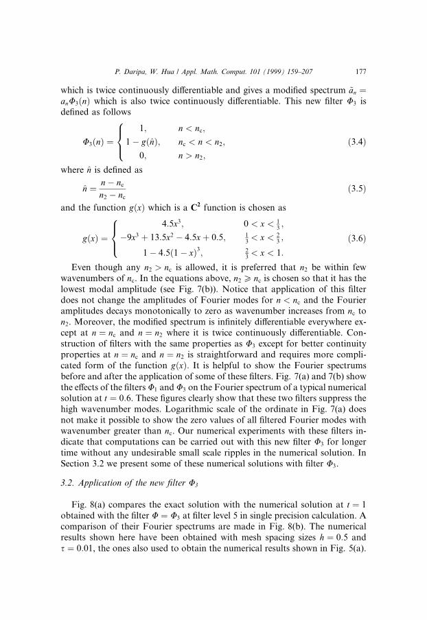
Even though any n2 > nc is allowed, it is preferred that n2 be within fewwavenumbers of nc. In the equations above, n2 P nc is chosen so that it has thelowest modal amplitude (see Fig. 7(b)). Notice that application of this ®lterdoes not change the amplitudes of Fourier modes for n < nc and the Fourieramplitudes decays monotonically to zero as wavenumber increases from nc ton2. Moreover, the modi®ed spectrum is in®nitely di�erentiable everywhere ex-cept at n � nc and n � n2 where it is twice continuously di�erentiable. Con-struction of ®lters with the same properties as U3 except for better continuityproperties at n � nc and n � n2 is straightforward and requires more compli-cated form of the function g�x�: It is helpful to show the Fourier spectrumsbefore and after the application of some of these ®lters. Fig. 7(a) and 7(b) showthe e�ects of the ®lters U1 and U3 on the Fourier spectrum of a typical numericalsolution at t � 0:6. These ®gures clearly show that these two ®lters suppress thehigh wavenumber modes. Logarithmic scale of the ordinate in Fig. 7(a) doesnot make it possible to show the zero values of all ®ltered Fourier modes withwavenumber greater than nc. Our numerical experiments with these ®lters in-dicate that computations can be carried out with this new ®lter U3 for longertime without any undesirable small scale ripples in the numerical solution. InSection 3.2 we present some of these numerical solutions with ®lter U3.
3.2. Application of the new ®lter U3
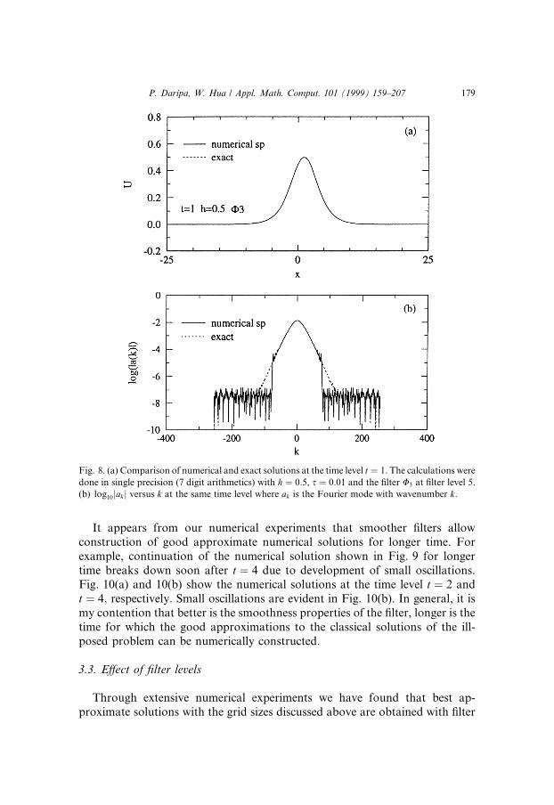
Fig. 8(a) compares the exact solution with the numerical solution at t � 1obtained with the ®lter U � U3 at ®lter level 5 in single precision calculation. Acomparison of their Fourier spectrums are made in Fig. 8(b). The numericalresults shown here have been obtained with mesh spacing sizes h � 0:5 ands � 0:01, the ones also used to obtain the numerical results shown in Fig. 5(a).
P. Daripa, W. Hua / Appl. Math. Comput. 101 (1999) 159±207 177

Comparison of these results with the ones in Fig. 5(a) where no ®lter is in useshows the e�ectiveness of this new ®lter in eliminating the spurious e�ect ofroundo� error.
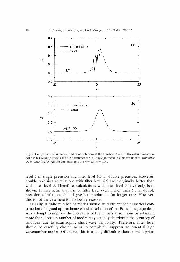
Fig. 9(a) shows the numerical solution at t � 1:7 obtained in double preci-sion calculations with no ®lter in use. A comparison of this numerical solutionwith the exact solution in this ®gure clearly shows the spurious small scaleripples, which is rather severe, in the numerical solution. Fig. 9(b) shows thenumerical solution obtained using the ®lter U3 in single precision at the sametime level. These numerical solutions in Fig. 9 should be compared with thenumerical solution shown in Fig. 6 which was obtained with the sharp ®lter U1
at ®lter level 5 at the same time level. It is quite clear that numerical resultsobtained with ®lter U3 are superior to the ones obtained with no ®lter or with®lters of lower order regularity such as U1 or U2.
Fig. 7. E�ectiveness of the ®lters (a) U1; (b) U3 in suppressing spurious growth of roundo� errors.
Fourier spectra of the numerical solutions at t � 0:6 before and after the use of the ®lters are
shown. The computations use h � 0:5, s � 0:01 at ®lter level 5. The Fourier spectrum of the exact
solution is also shown here for comparison purposes.
178 P. Daripa, W. Hua / Appl. Math. Comput. 101 (1999) 159±207
It appears from our numerical experiments that smoother ®lters allowconstruction of good approximate numerical solutions for longer time. Forexample, continuation of the numerical solution shown in Fig. 9 for longertime breaks down soon after t � 4 due to development of small oscillations.Fig. 10(a) and 10(b) show the numerical solutions at the time level t � 2 andt � 4; respectively. Small oscillations are evident in Fig. 10(b). In general, it ismy contention that better is the smoothness properties of the ®lter, longer is thetime for which the good approximations to the classical solutions of the ill-posed problem can be numerically constructed.
3.3. E�ect of ®lter levels
Through extensive numerical experiments we have found that best ap-proximate solutions with the grid sizes discussed above are obtained with ®lter
Fig. 8. (a) Comparison of numerical and exact solutions at the time level t � 1. The calculations were
done in single precision (7 digit arithmetics) with h � 0:5, s � 0:01 and the ®lter U3 at ®lter level 5.
(b) log10jak j versus k at the same time level where ak is the Fourier mode with wavenumber k.
P. Daripa, W. Hua / Appl. Math. Comput. 101 (1999) 159±207 179
level 5 in single precision and ®lter level 6.5 in double precision. However,double precision calculations with ®lter level 6.5 are marginally better thanwith ®lter level 5. Therefore, calculations with ®lter level 5 have only beenshown. It may seem that use of ®lter level even higher than 6.5 in doubleprecision calculations should give better solutions for longer time. However,this is not the case here for following reasons.
Usually, a ®nite number of modes should be su�cient for numerical con-struction of a good approximate classical solution of the Boussinesq equation.Any attempt to improve the accuracies of the numerical solutions by retainingmore than a certain number of modes may actually deteriorate the accuracy ofsolutions due to catastrophic short-wave instability. Therefore, ®lter levelshould be carefully chosen so as to completely suppress nonessential highwavenumber modes. Of course, this is usually di�cult without some a priori
Fig. 9. Comparison of numerical and exact solutions at the time level t � 1:7. The calculations were
done in (a) double precision (15 digit arithmetics); (b) single precision (7 digit arithmetics) with ®lter
U3 at ®lter level 5. All the computations use h � 0:5, s � 0:01.
180 P. Daripa, W. Hua / Appl. Math. Comput. 101 (1999) 159±207
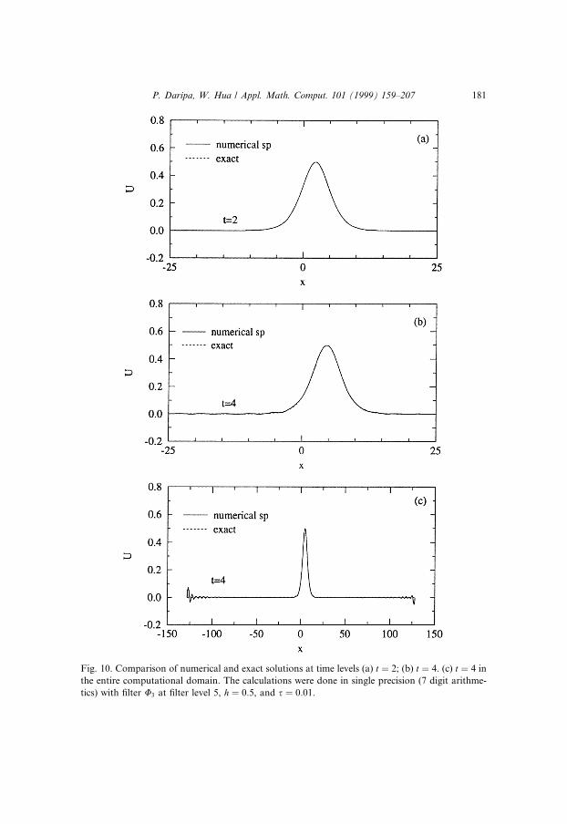
Fig. 10. Comparison of numerical and exact solutions at time levels (a) t � 2; (b) t � 4. (c) t � 4 in
the entire computational domain. The calculations were done in single precision (7 digit arithme-
tics) with ®lter U3 at ®lter level 5, h � 0:5, and s � 0:01.
P. Daripa, W. Hua / Appl. Math. Comput. 101 (1999) 159±207 181
knowledge of the solution itself. In most practical cases, some numericalexperiments will be necessary to be able to choose an ®lter optimal level forbest approximate solutions. Finally, it is important to be aware of the fact that®lter plays no role unless ®lter level is larger than the smallest amplitude of themodes participating in the numerical computations. Moreover, it may not al-ways be prudent to choose a ®lter level closer to the machine precision as thismay allow growth of spurious errors in many of the nonessential high wave-number modes.
4. Regularization methods
We brie¯y describe two regularization techniques. The Boussinesq equation(1.1) is modi®ed in these regularization techniques by adding appropriatehigher order terms to the right-hand side of the equation as discussed below.As we will see below, these modi®cations do not change the equilibrium statesuc or their characterization as elliptic or hyperbolic states. Therefore, the stateswith p0�uc� < 0 remain elliptic and states with p0�uc� > 0 remain hyperbolic inthese regularized equations.
Below we carry out linearized stability analysis of these regularized equa-tions and derive their dispersion relations. We further argue based on linear-ized stability analysis and physical consideration that surface-tension-likeregularization is more appropriate and is likely to give better approximatesolution. Moreover, it is easier here to implement the ®nite di�erence schemewith surface-tension-like regularization than with viscosity-like regularization.The numerical scheme of Section 2 is extended below for the regularizedequation with surface-tension-like regularization and linearized stability anal-ysis of the scheme is presented. Numerical results with this scheme are thenpresented. We ®nd that numerical solutions for modest values of regularizingparameters with appropriate ®lter can provide signi®cantly better approxi-mations to solutions of Eq. (1.1) than the ones obtained by ®ltering methodalone. Below we give more details on these issues.
4.1. First regularization technique
A simple way to regularize is to modify the Boussinesq equation (1.1) asfollows,
utt � �p�u��xx � uxxxx � duxxxxxx; d > 0: �4:1�
Below this equation is referred as MPDE1. The linearized pde correspondingto this regularized equation has decaying as well as growing modes, ert�ikx; withthe dispersion relation about the constant state, uc, given by
182 P. Daripa, W. Hua / Appl. Math. Comput. 101 (1999) 159±207
r� � �k����������������������������������k2 ÿ p0�uc� ÿ dk4
p; d > 0: �4:2�
It follows from this dispersion relation that there are no decaying or growingmodes, ert�ikx, unless
4p0�uc�d < 1: �4:3�The choice of d must satisfy Eq. (4.3) so that the dispersion relation (4.2) is
qualitatively similar to that for the original Boussinesq equation which hasboth growing and decaying modes. A simple calculation shows that the equi-librium states, uc, in the elliptic as well as hyperbolic region are unstable tomodes with wavenumbers in the interval �k1; k2� where k1 and k2 are given by
k21;2 � �1�
�������������������1ÿ 4p0d�
p=2d: �4:4�
The mode with the highest growth rate has wavenumber km�d� where
k2m � �1�
�������������������1ÿ 3p0d�
p=3d: �4:5�
Note that km�d� ! 1 as d! 0 which is consistent with the original Boussinesqequation.
Since all modes with wavenumber k P k2 have zero growth rate, the ill-posedness of the PDE is not present in this regularized equation. In the limitd! 0, the MPDE1 reduces to PDE (1.1) and the dispersion relation (4.2) ofthe MPDE1 reduces to that of the PDE. Therefore we have some con®dencethat the smooth solutions of the MPDE1 may converge to the smooth solu-tions of the PDE.
It is worth noting that for a ®xed choice of d > 0, the dispersion relation(4.2) of the MPDE1 is identical to that of the PDE in the long wave �k ! 0�approximation and is given by
r� � �k�����������������ÿp0�uc�;
pas k ! 0: �4:6�
These long waves travel at a speed � ���������������ÿp0�uc�p
regardless of the value of d inMPDE1. This also follows directly from the PDE and MPDE1 since in thislong wave approximation only the ®rst term in these equations is signi®cant.Therefore solutions of the MPDE1 and the PDE will not di�er much if theinitial data is a long wave perturbation about the constant equilibrium state.
There is only a ®nite number of modes which actually participate in a nu-merical calculation. Usually the highest wavenumber, kn, that participates in anumerical calculation with n grid points is O�n� (approximately n=4). Accuratenumerical simulation of the regularized Boussinesq equation (MPDE1) ispossible if enough grid points are used so that
kn > k� � akm �4:7�for some suitable choice of a > 1. A special choice of k� is k2. For choice ofk�P k2; the numerical scheme (2.1) will be able to resolve all modes which are
P. Daripa, W. Hua / Appl. Math. Comput. 101 (1999) 159±207 183
dynamically important (according to our linearized analysis). It follows fromEqs. (4.5) and (4.7) that
d >2
3
akn
� �2
1ÿ p0
2
akn
� �2 !
: �4:8�
Eqs. (4.3) and (4.8) give the following allowable values of d which are de-pendent on the choice of k� made in Eq. (4.7),
2
3
akn
1ÿ p0
2
akn
� �2 !
< d <1
4p0: �4:9�
Allowable values of d for a choice of k� � k2 in Eq. (4.7) are given by
1
kn
� �2
1ÿ p0
kn
� �2 !
< d <1
4p0: �4:10�
In Eq. (4.10), right inequality ensures that regularized and ill-posed Boussinesqequations have modes which are qualitatively similar and the inequality en-sures that instabilities of the shortest waves which the grid can resolve are mildso that numerical solution is not contaminated with the spurious growth ofroundo� error. For a speci®c choice of d, left inequality in Eq. (4.10) gives anestimate of the upper bound of the mesh size (mesh size is O�1=kn�). On theother hand, for a ®xed mesh size, however small, reliable numerical solution ofthe regularized equation is possible if d > d� where d� is the left inequality inEq. (4.10) which is approximately �1=kn�2 for small enough grid size orequivalently very large number of grid points. For choices of d < d�, ®lteringwill be necessary to eliminate the growth of spurious perturbations of shortwave amplitudes.
4.2. Finite di�erence scheme of MPDE1
The MPDE1 (4.1) is solved numerically using extension of the ®nite di�er-ence method discussed in Section 2.1, i.e. in a ®nite domain, a6 x6 b; for t > 0with uniform grid spacing h in x and s in t. The ®nite di�erence approximationto MPDE1 is then given by
D�t Dÿt vnj
s2� D�x Dÿx �p�vn
j ��h2
� �D�x Dÿx �2�vn�1
j � vnÿ1j �
2h4
� d�D�x Dÿx �3�vn�1
j � vnÿ1j �
2h6;
�4:11�
184 P. Daripa, W. Hua / Appl. Math. Comput. 101 (1999) 159±207

for s > 0 and 0 < j < N�06 j < N in case of periodic domain) where bÿ a �Nh: The truncation error is E�h; s� � O�h2� �O�s2�: Below this Eq. (4.11) isreferred as MFDE1. For non-periodic domain we need the same boundaryconditions and initialization given in Section 2.1. In addition, we also need twomore fourth order accurate boundary conditions since regularized equation isof higher order than the original Boussinesq equation. These two extraboundary conditions for n P 0 are given by
v�aÿ 2h; ns� � ÿ12v�a; ns� � 16v�a� h; ns�ÿ 3v�a� 2h; ns� ÿ 12v0�a; ns�h;
�4:12�
v�b� 2h; ns� � ÿ12v�b; ns� � 16v�bÿ h; ns� ÿ 3v�bÿ 2h; ns�ÿ 12v0�b; ns�h: �4:13�
The MFDE1 (4.11) is solved in an interval ÿ128 < x < 128 as before forvarious choice of d and subject to initial data us�x; 0� (see Eq. (1.5)) with am-plitude of the solitary wave A � 0:5: The boundaries are carefully chosen sothat they are far away from the support of the solitary wave for the duration ofthe computation.
4.3. Linearized stability of the MFDE1 about the constant states
Denoting the perturbation about the constant state, uc; by ~vnj ; and then
linearizing the MFDE1 about this constant state we obtain
D�t Dÿt ~vnj
k2� �p0�uc��
D�x Dÿx ~vnj
h2� �D
�x Dÿx �2�~vn�1
j � ~vnÿ1j �
2h4
� d�D�x Dÿx �3�~vn�1
j � ~vnÿ1j �
2h6:
�4:14�
With ~vnj � qneinj in Eq. (4.14). (where q � ebs; n � kh; k is the wavenumber and
real part of b is the growth rate), the dispersion relation for the numericalscheme is
Aq2 � 2Bq� A � 0; �4:15�where
A � 1ÿ 8r2 sin4 n2� 32dh2 sin6 n
2; B � 2k2p0�uc� sin2 n
2ÿ 1; �4:16�
where k � s=h; r � s=h2 and h � s=h3. Numerical scheme (4.11) should pref-erably use values of grid size s and h which allow the dispersion relation versusthe wavenumber k, best approximate the continuous dispersion relation over as
P. Daripa, W. Hua / Appl. Math. Comput. 101 (1999) 159±207 185

wide range of the spectrum as possible. Fig. 11 shows the plot of growth rateagainst the wavenumber k for two values of d when uc � 0: We have chosenh � 0:5 and s � 0:01 so that numerical results of this regularized equation canbe compared with those we have discussed in Sections 2 and 3. It is evidentfrom Fig. 11 that all modes with wavenumber k P k2 have zero growth ratewhich completely eliminates the short wavelength instabilities. It is importantto notice from Eqs. (4.2) and (4.3) that the constant state uc � 0 is neutrallystable for d > 0:25. Therefore the dispersion relations in this ®gure has beenshown for choices of d < 0:25 only.
4.4. Numerical results
We illustrate the e�ect of regularizing term by presenting numerical solu-tions of the regularized Boussinesq equation for several values of d. First weshould note from Eqs. (4.4) and (4.5) that most unstable wavenumber km andthe cuto� wavenumber k2 are O�1= ���
dp � as d! 0. Moreover, it follows from
Eqs. (4.2) and (4.5) that growth rate of the most unstable wave is given byr�km� � O�1=d� as d! 0. Therefore numerical di�culties due to machineroundo� error that we have discussed in Section 2 for the case d � 0 shouldalso occur for small values of d when computations are carried out with suf-®cient number of mesh points. As before, these di�culties for small values of dcan be overcome up to some ®nite time using either higher precision cal-culations or ®ltering techniques. We ®rst provide some calculations whend � 0:05; h � 0:5 and s � 0:01: For comparison purposes and clarity ofexposition of these numerical results, we ®rst show a single precision calcula-tion with d � 0:
Fig. 11. Dispersion relation for MPDE1 and MFDE1: Growth rate versus wavenumber k for
uc � 0:0, h � 0:5, s � 0:01 and two choices of d.
186 P. Daripa, W. Hua / Appl. Math. Comput. 101 (1999) 159±207
Fig. 12 compares the computed solutions of the ill-posed Boussinesqequation in 7 digit arithmetics (i.e. single precision) with its exact solutions attwo successive time levels. As previously discussed in Section 2, small scaleripples in the computed solution at t � 1 in Fig. 12(b) is due to ampli®cation ofthe amplitudes of short waves spuriously introduced by the machine roundo�error. This is seen in Fig. 12(c) where we have plotted logarithm of the Fouriercoe�cients' amplitudes against wavenumbers for these computed solutions. Itis worth recalling from Section 2 that Fourier coe�cients of the initial data(solitary wave) decay monotonically with wavenumber. However we see inFig. 12(c) that all participating modes with amplitudes smaller than 10ÿ7 insingle precision calculation are replaced by roundo� error of the order of 10ÿ7.The errors in the amplitudes of these short-waves which are many thousand-fold higher than their correct amplitudes get ampli®ed at later times by thesevere short-wave instability causing violent small scale oscillations to appearat t � 1 as seen in Fig. 12(c).
Figs. 13 and 14 show the numerical solutions of the regularized Boussinesqequation at successive time levels that were obtained in single and doubleprecision calculations respectively. These computations use d � 0:05; h � 0:5and s � 0:01. In these ®gures, numerical solutions for these time sequenceshave also been compared with exact solutions of the ill-posed Boussinesqequation. The computed solutions of the regularized equation (4.1) for earliertimes have not been shown in these ®gures because these solutions not onlycontain no irregularities but also compare very well with the exact solutionsus�x; t� of the ill-posed equation (1.1).
Very small irregularities that appear in the numerical solution at t � 1:7 inFig. 13(b) is largely due to ampli®cation of spurious perturbation in the am-plitudes of short waves introduced by machine round o� error and not due tosmall nonzero value of d. This is seen in Fig. 13(c) where we have plottedlogarithm of the Fourier coe�cients' amplitudes against the wavenumbers. Weshould recall that Fourier coe�cients of the initial data decay monotonicallywith wavenumber. However we see in Fig. 13(c) that all participating modeswith amplitudes smaller than 10ÿ7 in single precision calculation are replacedby roundo� error of the order of 10ÿ7. The errors in the amplitudes of theseshort-waves which are many thousand-fold higher than their correct ampli-tudes get ampli®ed at later times due to their severe growth rate at such a smallvalue of d. This causes the irregularities in the numerical solution shown inFig. 13(b). However, these irregularities could have been much worse if it werenot for the small value of the regularizing parameter d. A comparison of thenumerical solutions in Figs. 12 and 13 show this. A comparison of the Fourierspectrums of these solutions in Fig. 12(c) and Fig. 13(c) clearly show the e�ectsof nonzero values of d in reducing the growth rate of the short-wave compo-nents of roundo� error and thereby providing better approximate solutions ofthe ill-posed Boussinesq equation.
P. Daripa, W. Hua / Appl. Math. Comput. 101 (1999) 159±207 187

Fig. 12. Computed solutions of the ill-posed Boussinesq equation at time levels t � 0:8 and t � 1:0.
The calculations use h � 0:5, s � 0:01 and were done in single precision (7 digit arithmetics). (c)
Logarithm � log10� of the Fourier coe�cients' amplitudes against the wavenumber k for the initial
data and the computed solutions.
188 P. Daripa, W. Hua / Appl. Math. Comput. 101 (1999) 159±207
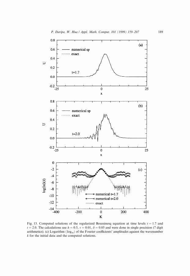
Fig. 13. Computed solutions of the regularized Boussinesq equation at time levels t � 1:7 and
t � 2:0. The calculations use h � 0:5, s � 0:01, d � 0:05 and were done in single precision (7 digit
arithmetics). (c) Logarithm � log10� of the Fourier coe�cients' amplitudes against the wavenumber
k for the initial data and the computed solutions.
P. Daripa, W. Hua / Appl. Math. Comput. 101 (1999) 159±207 189

Fig. 14. Computed solutions of the regularized Boussinesq equation at time levels t � 1:7 and
t � 2:0. The calculations use h � 0:5, s � 0:01, d � 0:05 and were done in double precision (15 digit
arithmetics). (c) Logarithm � log10� of the Fourier coe�cients' amplitudes against the wavenumber
k for the initial data and the computed solutions.
190 P. Daripa, W. Hua / Appl. Math. Comput. 101 (1999) 159±207

Higher precision calculations provide even better approximate solutionsdue to less roundo� error. In this regard, single precision calculations ofFig. 13 should be compared with the double precision calculations of Fig. 14where all participating modes have amplitudes larger than the machine pre-cision and therefore no irregularities appear in the numerical solutions. Thisfurther supports our earlier contention that the irregularities of Fig. 13(b) isdue to the roundo� error and not due to nonzero value of d � 0:05. Forreasons discussed earlier, e�ect of roundo� error for even higher precisioncalculations here is marginal unless computations are carried out on ®nermesh sizes.
We have seen in Section 3 that an alternative to using high precision cal-culations to improve numerical accuracy is to use ®ltering technique with lowerprecision calculations. We have experimented with the three ®lters discussedearlier in Section 3 and have found the ®lter U3 to perform the best at ®lterlevel 5 in single precision calculations. We recall that this ®lter replaces all theFourier modes having amplitudes less than 10ÿ5 with modi®ed values of am-plitudes less than 10ÿ5 such that the modi®ed spectrum, i.e. Fourier modes'amplitudes versus the wavenumber curve, is a rapidly decaying C2 function.E�ect of this ®lter is to set most of these Fourier modes' amplitudes to zeroexcept a very few ones closest to the cuto� wavenumber whose amplitudesrapidly decay to zero from 10ÿ5. Single precision calculations using this ®lterare shown in Fig. 15. This should be compared with single and double preci-sion results of Figs. 13 and 14. A comparison of the Fourier spectrums of thesesolutions in these ®gures show the e�ectiveness of the ®lter in suppressing thegrowth of spurious perturbations introduced by machine precision. Moreover,we see considerable improvements in the accuracy of the computed solutionsusing this ®lter.
Numerical experiments for various choices of d indicate that good ap-proximate solutions of the ill-posed Boussinesq equation can be obtained withrather large values of d. Fig. 16 shows that numerical solutions with d � 0:25are signi®cantly better approximations to the exact solutions of Eq. (1.1) thanthose we obtained earlier with the ®ltering technique alone. It is worth recallingthat the null state for the regularized equation is neutrally stable exactly atd � 0:25.
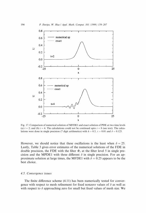
Fig. 17 shows the case when d � 0:125. Here the numerical solutions at twotime levels are shown only. The oscillations in the numerical solution at t � 4in 17(b) quickly grow and does not allow any meaningful solution for latertimes to be computed. Fig. 18 shows the other extreme when d � 1. The shift ismore severe and oscillations occur at the right-hand side (not left-hand side aswe saw in Fig. 17(b)) of the solitary wave. We do not know whether theseoscillations are properties of the solutions of the regularized equation or arepurely a result of numerical artifacts such as phase error. We do not seek toresolve this issue here and hope to consider this issue in our future work.
P. Daripa, W. Hua / Appl. Math. Comput. 101 (1999) 159±207 191
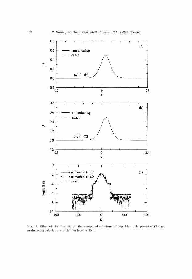
Fig. 15. E�ect of the ®lter U3 on the computed solutions of Fig. 14: single precision (7 digit
arithmetics) calculations with ®lter level at 10ÿ5.
192 P. Daripa, W. Hua / Appl. Math. Comput. 101 (1999) 159±207

Fig. 16. Comparison of numerical solution of MFDE1 and exact solution of PDE at di�erent time
levels (a) t � 2; (b) t � 4; and (c) t � 8. The calculations were done in single precision (7 digit
arithmetics) with h � 0:5, s � 0:01 and d � 0:25:
P. Daripa, W. Hua / Appl. Math. Comput. 101 (1999) 159±207 193
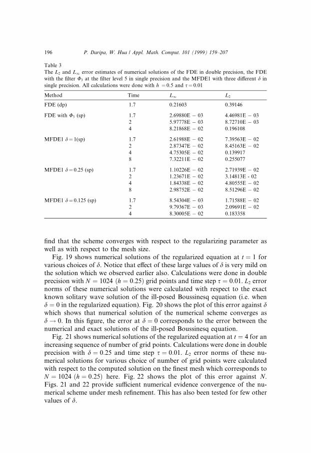
However, we should notice that these oscillations is the least when d � 25.Lastly, Table 3 gives error estimates of the numerical solutions of the FDE indouble precision, the FDE with the ®lter U3 at the ®lter level 5 in single pre-cision and the MPDE1 with three di�erent d in single precision. For an ap-proximate solution at large times, the MFDE1 with d � 0:25 appears to be thebest choice.
4.5. Convergence issues
The ®nite di�erence scheme (4.11) has been numerically tested for conver-gence with respect to mesh re®nement for ®xed nonzero values of d as well aswith respect to d approaching zero for small but ®xed values of mesh size. We
Fig. 17. Comparison of numerical solution of MFDE1 and exact solution of PDE at two time levels
(a) t � 2; and (b) t � 4. The calculations could not be continued upto t � 8 (see text). The calcu-
lations were done in single precision (7 digit arithmetics) with h � 0:5, s � 0:01 and d � 0:125:
194 P. Daripa, W. Hua / Appl. Math. Comput. 101 (1999) 159±207
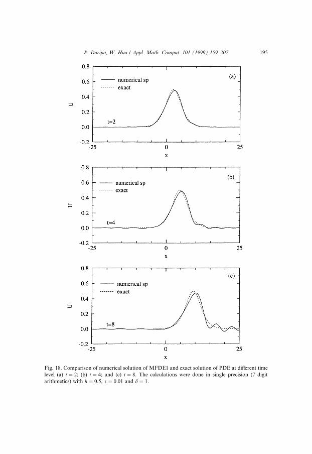
Fig. 18. Comparison of numerical solution of MFDE1 and exact solution of PDE at di�erent time
level (a) t � 2; (b) t � 4; and (c) t � 8. The calculations were done in single precision (7 digit
arithmetics) with h � 0:5, s � 0:01 and d � 1:
P. Daripa, W. Hua / Appl. Math. Comput. 101 (1999) 159±207 195
®nd that the scheme converges with respect to the regularizing parameter aswell as with respect to the mesh size.
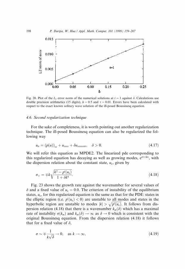
Fig. 19 shows numerical solutions of the regularized equation at t � 1 forvarious choices of d. Notice that e�ect of these large values of d is very mild onthe solution which we observed earlier also. Calculations were done in doubleprecision with N � 1024 �h � 0:25� grid points and time step s � 0:01. L2 errornorms of these numerical solutions were calculated with respect to the exactknown solitary wave solution of the ill-posed Boussinesq equation (i.e. whend � 0 in the regularized equation). Fig. 20 shows the plot of this error against dwhich shows that numerical solution of the numerical scheme converges asd! 0. In this ®gure, the error at d � 0 corresponds to the error between thenumerical and exact solutions of the ill-posed Boussinesq equation.
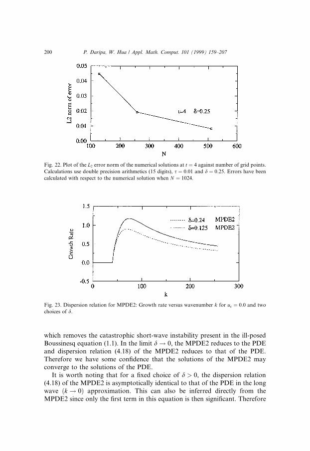
Fig. 21 shows numerical solutions of the regularized equation at t � 4 for anincreasing sequence of number of grid points. Calculations were done in doubleprecision with d � 0:25 and time step s � 0:01. L2 error norms of these nu-merical solutions for various choice of number of grid points were calculatedwith respect to the computed solution on the ®nest mesh which corresponds toN � 1024 �h � 0:25� here. Fig. 22 shows the plot of this error against N.Figs. 21 and 22 provide su�cient numerical evidence convergence of the nu-merical scheme under mesh re®nement. This has also been tested for few othervalues of d.
Table 3
The L2 and L1 error estimates of numerical solutions of the FDE in double precision, the FDE
with the ®lter U3 at the ®lter level 5 in single precision and the MFDE1 with three di�erent d in
single precision. All calculations were done with h � 0.5 and s� 0.01
Method Time L1 L2
FDE (dp) 1.7 0.21603 0.39146
FDE with U3 (sp) 1.7 2.69880E ÿ 03 4.46981E ÿ 03
2 5.97778E ÿ 03 8.72710E ÿ 03
4 8.21868E ÿ 02 0.196108
MFDE1 d� 1(sp) 1.7 2.61988E ÿ 02 7.39563E ÿ 02
2 2.87347E ÿ 02 8.45163E ÿ 02
4 4.75305E ÿ 02 0.139917
8 7.32211E ÿ 02 0.255077
MFDE1 d� 0.25 (sp) 1.7 1.10226E ÿ 02 2.71939E ÿ 02
2 1.23671E ÿ 02 3.14813E - 02
4 1.84338E ÿ 02 4.80555E ÿ 02
8 2.98752E ÿ 02 8.51296E ÿ 02
MFDE1 d� 0.125 (sp) 1.7 8.54304E ÿ 03 1.71588E ÿ 02
2 9.79367E ÿ 03 2.09691E ÿ 02
4 8.30005E ÿ 02 0.183358
196 P. Daripa, W. Hua / Appl. Math. Comput. 101 (1999) 159±207
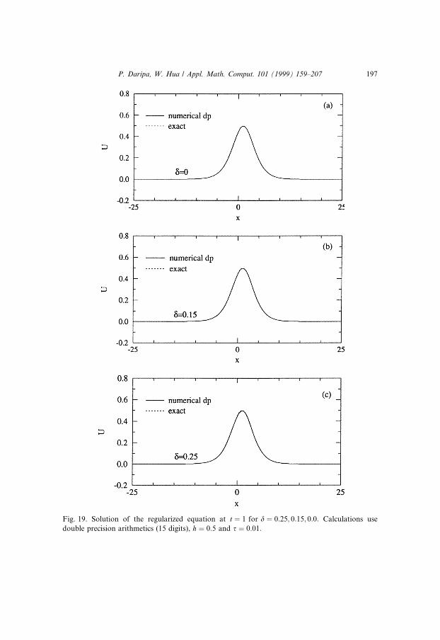
Fig. 19. Solution of the regularized equation at t � 1 for d � 0:25; 0:15; 0:0: Calculations use
double precision arithmetics (15 digits), h � 0:5 and s � 0:01:
P. Daripa, W. Hua / Appl. Math. Comput. 101 (1999) 159±207 197
4.6. Second regularization technique
For the sake of completeness, it is worth pointing out another regularizationtechnique. The ill-posed Boussinesq equation can also be regularized the fol-lowing way
utt � �p�u��xx � uxxxx � duxxxxxxtt; d > 0: �4:17�We will refer this equation as MPDE2. The linearized pde corresponding tothis regularized equation has decaying as well as growing modes, ert�ikx, withthe dispersion relation about the constant state, uc, given by
r� � �k
����������������������k2 ÿ p0�uc�
1� dk6
r: �4:18�
Fig. 23 shows the growth rate against the wavenumber for several values ofd and a ®xed value of uc � 0:0. The criterion of instability of the equilibriumstates, uc, for this regularized equation is the same as that for the PDE: states inthe elliptic region (i.e. p0�uc� < 0� are unstable to all modes and states in thehyperbolic region are unstable to modes jkj > ������������
p0�uc�p
. It follows from dis-persion relation (4.18) that there is a wavenumber km�d� which has a maximalrate of instability r�km� and km�d� ! 1 as d! 0 which is consistent with theoriginal Boussinesq equation. From the dispersion relation (4.18) it followsthat for a ®xed value of d,
r � � 1
k���dp ! 0; as k !1; �4:19�
Fig. 20. Plot of the L2 error norm of the numerical solutions at t � 1 against d. Calculations use
double precision arithmetics (15 digits), h � 0:5 and s � 0:01. Errors have been calculated with
respect to the exact known solitary wave solution of the ill-posed Boussinesq equation.
198 P. Daripa, W. Hua / Appl. Math. Comput. 101 (1999) 159±207
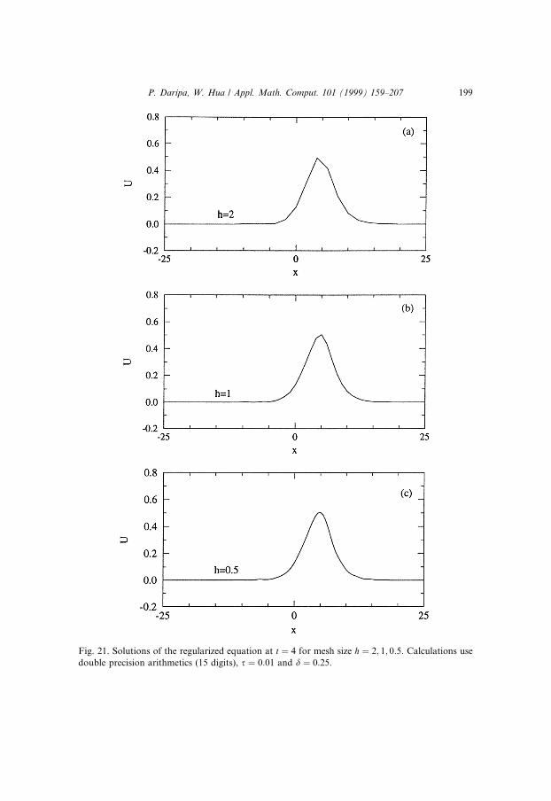
Fig. 21. Solutions of the regularized equation at t � 4 for mesh size h � 2; 1; 0:5: Calculations use
double precision arithmetics (15 digits), s � 0:01 and d � 0:25.
P. Daripa, W. Hua / Appl. Math. Comput. 101 (1999) 159±207 199
which removes the catastrophic short-wave instability present in the ill-posedBoussinesq equation (1.1). In the limit d! 0, the MPDE2 reduces to the PDEand dispersion relation (4.18) of the MPDE2 reduces to that of the PDE.Therefore we have some con®dence that the solutions of the MPDE2 mayconverge to the solutions of the PDE.
It is worth noting that for a ®xed choice of d > 0, the dispersion relation(4.18) of the MPDE2 is asymptotically identical to that of the PDE in the longwave �k ! 0� approximation. This can also be inferred directly from theMPDE2 since only the ®rst term in this equation is then signi®cant. Therefore
Fig. 22. Plot of the L2 error norm of the numerical solutions at t � 4 against number of grid points.
Calculations use double precision arithmetics (15 digits), s � 0:01 and d � 0:25. Errors have been
calculated with respect to the numerical solution when N � 1024.
Fig. 23. Dispersion relation for MPDE2: Growth rate versus wavenumber k for uc � 0:0 and two
choices of d.
200 P. Daripa, W. Hua / Appl. Math. Comput. 101 (1999) 159±207
solutions of the MPDE2 and the PDE may not di�er much if the initial dataare a long wave perturbation about the constant equilibrium state.
If for some suitable a > 1; kn > akm is the largest wavenumber that partic-ipates in a numerical scheme for a particular choice of d; then according to thedispersion relation participating short-waves will have small growth rate.Therefore, the numerical scheme will produce numerical solutions which areless likely to be contaminated with machine roundo� error. As d! 0, both km
and kn approach in®nity which may cause catastrophic growth of spuriousperturbations if computations are carried out on small enough mesh size. Ingeneral, ®ltering as well as regularization will be necessary for numericalcomputation of good approximate solutions of the ill-posed equation in thelimit d! 0.
It is evident from the dispersion relation here that the regularization term inEq. (4.17) reduces the growth rates of all short waves such that growth rate ofshort waves vanishes asymptotically which is very reminiscent of the dampingusually provided by viscosity in ¯uid ¯ow contexts. Even though this regu-larization reduces the spurious e�ect of roundo� error, it may cause signi®cantattenuation of the solutions, a fact not unusual with viscosity like damping.Therefore, this alternative regularization, even though a viable alternative, isunlikely to be superior to the surface-tension like regularization of the ®rstmethod we discussed earlier in detail. Hence we have not implemented thismethod, as mentioned right in the beginning of this section. This regularizationmethod is mentioned here for the sake of discussion and may be implementedby any of the readers, if so desired.
5. Summary
A ®nite di�erence scheme for solving an ill-posed Boussinesq equation hasbeen proposed and numerically investigated. The scheme is then used to ex-emplify the di�culties of computing good approximate solutions of thisequation due to catastrophic short-wave instabilities; and to develop appro-priate ®ltering and regularization methods in order to deal with these numer-ical di�culties. Numerical results indicate that the scheme is convergent andgrowth of errors can be controlled with suitable ®ltering and regularizationtechniques. A rigorous proof of the convergence of the numerical scheme is atopic of future work.
The ®nite di�erence scheme that we have proposed here is suitable forstudying initial value problems with arbitrary boundary data. However, it maybe worth pointing out that this scheme may su�er from some amount of phaseerror. Spectral ®ltering technique that we have used here is ideal for periodicdata and may require some modi®cation for its use with nonperiodic data
P. Daripa, W. Hua / Appl. Math. Comput. 101 (1999) 159±207 201

which is as yet another topic of research. For our choices of time and spaceintervals in the examples presented, the support of solitary wave remains formost examples far away from the boundaries and the data remains periodicwithin an error of the order of machine precision. Therefore, use of spectral®ltering to address issues related to the control of growth of error due to short-wave instability is justi®ed.
Numerical di�culties in computing good approximate solutions can arisedue to truncation as well as roundo� errors. We have shown that loss of nu-merical accuracy is largely due to truncation error when amplitudes of theparticipating modes are greater than the roundo� error (see Fig. 4). However,roundo� error becomes a major source of numerical di�culty when some ofthe high wavenumber participating modes have amplitudes much smaller thanthe roundo� error (see Fig. 5). In this situation, these modes are misrepre-sented during computation with an amplitude of the order of roundo� errorwhich is signi®cantly higher than the actual amplitudes of these modes in arelative sense. For example, the ratio of roundo� error to the amplitude of thehighest participating mode in Fig. 5 is approximately 107! A relative error ofsuch a high magnitude gets ampli®ed by the severe short-wave instabilityduring computation resulting in signi®cant loss of accuracy within a very shorttime. Increasing machine precision can improve the numerical solutions underthese circumstances only up to a point until some high wavenumber partici-pating modes attain amplitudes smaller than the roundo� error. Even if theroundo� error is brought under control with high precision arithmetics, theerror in the high wavenumber modes due to truncation error which gets am-pli®ed signi®cantly by the severe short wave instability of this problem canseriously deteriorate the accuracy of the numerical solution as we have seen inFig. 4. Finer mesh sizes may reduce the truncation error but may exacerbatethe numerical di�culties due to new high wavenumber modes that come intoplay. Therefore construction of good approximate solutions requires control ofboth of these types of error.
We have used two common techniques often used in constructing approxi-mate solutions to ill-posed problems: ®ltering techniques and regularizationtechniques (see [14]). In ®ltering technique, the data are appropriately perturbedso that the numerical solution of this modi®ed problem is a better approxi-mation to the solution of the original problem. The practice of perturbing thedata by locally averaging the solution in physical space is most common e.g.Rayleigh±Taylor [15], porous media ¯ow [3]. However, the data can also beperturbed by modifying its Fourier spectrum. Most often modi®cation of thedata in physical space is somewhat ad hoc and therefore whenever possible, it ispreferable to appropriately modify the Fourier spectrum of the data. Moreover,there are at least two advantages to this: (i) spurious oscillations due to theroundo� and truncation errors appear sooner in Fourier space than in physicalspace allowing earlier control of these errors; and (ii) suitable ®lters can be
202 P. Daripa, W. Hua / Appl. Math. Comput. 101 (1999) 159±207
constructed and applied at appropriate ®lter level to selectively control roundo�and truncation errors. Therefore we have chosen to apply the ®ltering techniquein Fourier space. Use of Spectral ®ltering technique has also been partly mo-tivated by its success in works of Krasny [7,8] and Shelly [11].
We have experimented with three types of ®lters with increasing order ofregularity and have found that best results were obtained with the ®lter whichis most regular. We introduced a new ®lter U3 (see Eq. (3.4)) which is a twicecontinuously di�erentiable function of the wavenumber k. This new ®lter hasthe property that the modi®ed spectrum after its application remains twicecontinuously di�erentiable. Choice of ®lter level is also crucial. With appro-priate choice of ®lter level, ®ltered computations can be remarkably better thanhigher precision un®ltered computations (see Fig. 10 and 9(a)). We have foundthat such an optimal choice of ®lter level should be somewhat higher (sometimesigni®cantly higher as in our double precision calculation where ®lter level 5 todoes better than ®lter level 12) than the machine precision level. This eliminatesmany high wavenumber modes which may contaminate the solutions by am-plifying roundo� errors in these modes rather than improving the accuracy ofthese solutions.
In regularization technique the equation, instead of the data, is appropri-ately perturbed so that the numerical solution of this modi®ed equation is abetter approximation to the solution of the original problem. We have showntwo ways to perturb the equation by adding a higher order derivative term tothe equation. In one approach, it completely eliminates all waves beyond acertain cut-o� wavenumber which depends on the small parameter in thehighest order derivative term in the equation. This kind of damping is similarto the one usually provided by surface tension. In the other approach, it mildlydampens the growth rate of most waves in such a way that growth rate decaysasymptotically to zero with wavenumber. This damping is similar to the oneusually provided by viscosity. We have argued in favor of surface-tension-likeregularization and extended the ®nite di�erence scheme of the original equa-tion for solving the regularized equation with this kind of regularization. Thecalculations seem to indicate that appropriate choices of parameter values inthe regularized equations can provide good approximate solutions of the ill-posed Boussinesq equation at least up to some ®nite time. Our results indicatethat better approximate solutions are obtained with regularization than with®ltering technique alone. Regularization with ®ltering further improves theaccuracy of the solutions.
It is worth pointing out that we are not aware of any numerical work on thisill-posed problem. This present numerical work illustrates only some of thedi�culties associated with this equation. In closing we should mention some ofthe interesting problems which may be worth considering as areas of futurework: (i) rigorous convergence proof of the ®nite di�erence schemes presentedin this work; (ii) a study of the structural stability of the solitary wave solution;
P. Daripa, W. Hua / Appl. Math. Comput. 101 (1999) 159±207 203

(iii) a study of the issues discussed in this paper using other numericalmethods such as spectral method; (iv) a systematic numerical study of ap-propriate initial value problems for the ill-posed and regularized Boussinesqequations; and (v) A numerical study of blow-up and formation of singularitiesin this equation.
Acknowledgements
The ®rst author (Prabir Daripa) is grateful to Marsha Berger for her hos-pitality at Courant Institute. P.D. would like to thank Peter Lax and Joh-nathan Goodman of Courant Institute for sharing their ideas.
Appendix A. Shallow water theory: Long waves
We brie¯y describe how the ill-posed Boussinesq equation (1.1) arises in thecontext of water waves. In doing so, we closely follow Chapter 13 of [16]. Iftime is denoted by t, the space coordinates by �x; y; z�, the gravitational ac-celeration acting in negative y direction by g, the density of ¯uid by q, thepressure in the water by p, the velocity potential in the water by / introducedthrough the velocity u � r/ due to irrationality, surface of the water wave byy � g�x; z; t�; and the bottom of constant depth by y � ÿh0, then the followingequations describe the motion of water in a region X subject to an appropriateinitial data.
D/ � 0; in X;
p ÿ p0
q� ÿ/t ÿ
1
2�jr/j�2 ÿ gy; in X;
gt � /xgx � /zgz � /y ; on y � g�x; z; t�;/t �
1
2�jr/j�2 � gg � 0; on y � g�x; z; t�;
/y � 0; on y � ÿh0:
�A:1�
The e�ect of surface tension has been neglected in the above equations. Thelinearized version of the above system about an initially rest state of watersupport waves of the form (see [16])
g � Aeik�xÿixt; / � Y �y�eik�xÿixt �A:2�
with the dispersion relation given by x2 � gk tanh kh0 where k is the magnitudeof the wave vector k i.e. k � jkj. Therefore the initial value problem associatedwith the system (A.1) is linearly well-posed.
204 P. Daripa, W. Hua / Appl. Math. Comput. 101 (1999) 159±207
It should be noted that the dispersive e�ects drop out in the long waveapproximation due to the fact that x2 � gh0k2; as kh0 ! 0 and therefore alllong waves in the linear regime travel at the same phase speed c0 �
�������gh0
p. The
nondispersive e�ects in this linear regime within long wave approximationinhibit wave breaking phenomena. Wave breaking phenomena can be capturedby incorporating higher order e�ects of the long wave approximation. One ofthe ways this is achieved is by setting up a more formal expansion of the system(A.1) in the small parameter �kh0�2 or equivalently in �h0=l�2 where l is thewavelength. As derived in [16] in some detail, a nonlinear approximation tosystem (A.1) which is correct up to the order O�kh0�4 is given by the followingsystem for one-dimensional waves traveling in the x direction with u being the¯uid velocity in this x direction. Below we have used h � h0 � g.
ht � �uh�x � 0; ut � uux � ghx � 1
3c2
0h0hxxx � 0: �A:3�The linearized version of the system (A.3) about the rest state is given by
gtt ÿ c20gxx ÿ
1
3c2
0h20gxxxx � 0; �A:4�
which has the dispersion relation
x2 � c20k2 ÿ 1
3c2
0h20k4: �A:5�
It should be noticed that under the scaling t! �h0=�������3c0
p �t and x! �h0=���3p �x;
Eq. (A.4) reduces to
gtt � gxx � gxxxx: �A:6�
This is the linearized version of the ill-posed Boussinesq equation (1.1) whichincorporates the quadratic nonlinearity of Eq. (A.3).
The dispersion relation (A.5) shows that the system (A.3) is linearly ill-posedand waves with �kh0�2 < 3 are ampli®ed. To make the study of this equationcomputationally feasible, an understanding as to how to bring the spuriousgrowth of errors under control as well as some sort of meaningful modi®cationof this equation are required.
One well-posed variants of Eqs. (A.3) and (A.4) favored by Boussinesq [16]are respectively
ht � �uh�x � 0; ut � uux � ghx � 1
3h0hxtt � 0 �A:7�
and
gtt ÿ c20gxx ÿ
1
3h2
0gxxtt � 0 �A:8�
P. Daripa, W. Hua / Appl. Math. Comput. 101 (1999) 159±207 205
with the dispersion relation given by
x2 � c20k2
1� �1=3�k2h20
: �A:9�
These equations follow directly from the lowest order approximations (e.g.replace gxx by gtt=c2
0 in Eq. (A.4)) and do not modify the long-wave dispersionrelation.
The problem with Eq. (A.8) is that it does not allow, at least in an obviousmanner, understanding of Eq. (A.4) or its solutions. Moreover, it has neverbeen shown that the solutions of Eq. (A.8) in any way approximate solutions ofEq. (A.4). It is intuitively more appropriate to regularize Eq. (A.4) in a way thatretains its long wave dispersion relation, provides good approximate solutionsof Eq. (A.4) when these exist (see Section 4) and provides a hope give to betterinsight into this equation and its solutions in the some appropriate limit of theregularizing parameter. To achieve these goals it is also essential to explorepossible ways, if any, to control the severe growth of numerical errors (seeSection 3). Important mathematical issues related to this equation which can-not be answered analytically can possibly then be addressed by computation.
References
[1] M. A�ouf, R.E. Ca¯isch, A numerical study of reimann problems solutions and stability for a
system of viscous conservation laws of mixed type, SIAM J. Appl. Math. 51 (3) (1991) 605±
634.
[2] G. Baker, D.I. Meiron, S.A. Orszag, Vortex simulations of the Rayleigh-Taylor instability,
Phys. Fluids 23 (1980) 1485±1488.
[3] P. Daripa, J. Glimm, B. Lindquist, O. McBryan, Polymer ¯oods: A case study of nonlinear
wave analysis and of instability control in tertiary oil recovery, SIAM J. Appl. Math. 48 (1988)
353±373.
[4] P. Deift, C. Tomei, E. Trubowitz, Inverse scattering and the Boussinesq equation, Comm. Pure
Appl. Math. 35 (1982) 567±628.
[5] R. Hirota, Exact N-soliton solutions of the wave equation of long waves in shallow-water and
in nonlinear lattices, J. Math. Phys. 14 (1973) 810±815.
[6] T.Y. Hou, J. Lowengrub, R. Krasny, Convergence of a point vertex method for vertex sheets,
SIAM J. Num. Anal. 28 (1991) 308±320.
[7] R. Krasny, A study of singularity formation in a vortex sheet by the point vortex
approximation, J. Fluid Mech. 167 (1986) 65±93.
[8] R. Krasny, Desingularization of periodic vortex sheet roll-up, J. Comput. Phys. 65 (1986) 292±
313.
[9] V.S. Manoranjan, A.R. Mitchell, J. Li, Morris, Numerical solution of the good Boussinesq
equation, SIAM J. Sci. Stat. Comput. 5 (1985) 946±957.
[10] A.C. Scott, F.Y.F. Chu, D.W. Mclaughlin, The soliton: A new concept in applied science,
Proc. IEEE 61 (10) (1973) 1443±1483.
[11] M.J. Shelley, A study of singularity formation in vortex-sheet motion by a spectrally accurate
vortex method, J. Fluid Mech. 244 (1992) 493±526.
206 P. Daripa, W. Hua / Appl. Math. Comput. 101 (1999) 159±207

[12] M. Slemrod, Admissibility criteria for propagating phase boundaries in a van der Walls ¯uid,
Arch. Rational Mech. Anal. 81 (1983) 301±315.
[13] M. Slemrod, Dynamic phase transition in a van der Waals ¯uid, J. Di�erential Equations 52
(1984) 1±23.
[14] A.N. Tikhonov, V.Y. Arsenin, Solutions of Illposed Problems, Translated by Fritz John,
Wiley, New York, 1977.
[15] G. Tryggvason, Numerical simulations of the Rayleigh-Taylor instabilities, J. Comput. Phys.
80 (1989) 1±16.
[16] G.B. Whitham, Linear and Nonlinear Waves, Wiley, New York, 1974.
[17] V.E. Zhakarov, On stochastization of one-dimensional chains of nonlinear oscillation, Sov.
Phys. JETP 38 (1) (1974) 108±110.
P. Daripa, W. Hua / Appl. Math. Comput. 101 (1999) 159±207 207