A numerical model for the dynamic simulation of a

HAL Id: hal-00713904https://hal.archives-ouvertes.fr/hal-00713904

Submitted on 3 Oct 2013

HAL is a multi-disciplinary open accessarchive for the deposit and dissemination of sci-entific research documents, whether they are pub-lished or not. The documents may come fromteaching and research institutions in France orabroad, or from public or private research centers.

L’archive ouverte pluridisciplinaire HAL, estdestinée au dépôt et à la diffusion de documentsscientifiques de niveau recherche, publiés ou non,émanant des établissements d’enseignement et derecherche français ou étrangers, des laboratoirespublics ou privés.

A numerical model for the dynamic simulation of arecirculation single-effect absorption chiller

Matthieu Zinet, Romuald Rulliere, Philippe Haberschill

To cite this version:Matthieu Zinet, Romuald Rulliere, Philippe Haberschill. A numerical model for the dynamic simula-tion of a recirculation single-effect absorption chiller. Energy Conversion and Management, Elsevier,2012, 62, pp.51-63. �10.1016/j.enconman.2012.04.007�. �hal-00713904�

https://hal.archives-ouvertes.fr/hal-00713904

https://hal.archives-ouvertes.fr

A Numerical Model for the Dynamic Simulation of a Recirculation Single-

Effect Absorption Chiller

Matthieu ZINET, Romuald RULLIERE*, Philippe HABERSCHILL

Université de Lyon, CNRS

INSA-Lyon, CETHIL, UMR 5008, F-69621, Villeurbanne, France

Université Lyon 1, F-69622, France

*corresponding author: Tel. +33 4 72 43 63 05 – Fax. +33 4 72 43 88 11

*E-mail address: [email protected]

Abstract

A dynamic model for the simulation of a new single-effect water/lithium bromide absorption

chiller is developed. The chiller is driven by two distinct heat sources, includes a custom

integrated falling film evaporator-absorber, uses mixed recirculation and is exclusively cooled

by the ambient air. Heat and mass transfer in the evaporator-absorber and in the desorber are

described according to a physical model for vapour absorption based on Nusselt’s film theory.

The other heat exchangers are handled using a simplified approach based on the NTU-

effectiveness method. The model is then used to analyze the chiller response to a step drop of

the heat recovery circuit flow rate, and to a sudden reduction of the cooling need in the

conditioned space. In the latter case, a basic temperature regulation system is simulated. In

both simulations, the performance of the chiller is well represented and consistent with

expectations.

Keywords: absorption; chiller; modelling; transient; water-lithium bromide; falling film

Nomenclature

Symbol Designation Unit

Variables – Latin letters

a film thickness parameter -

c molar concentration mol.m-3

C heat capacity rate W.K-1

Cp specific heat capacity J.kg-1.K

-1

D diffusion coefficient m2.s

-1

e Wall thickness m

g gravitational acceleration m.s-2

G& mass flow rate per film unit width kg.s-1.m

-1

h specific enthalpy J.kg-1

k thermal conductivity W.m-1.K

-1

L length m

M mass kg

M% molar weight g.mol-1

m& mass flow rate kg.s-1

NT Nusselt film thickness parameter -

NTU number of transfer units -

p pressure kPa

Q& heat flux W.m-2

Re Reynolds number -

S area m2

t time s

T temperature °C

u specific internal energy J.kg-1

U total internal energy J

UA overall heat transfer coefficient W.m-2.K

-1

v velocity m.s-1

V volume m3

x LiBr mass fraction kg.m-3

y film coordinate in the thickness direction m

Z liquid level m

Variables - Greek letters

α heat transfer coefficient W.m-2.K

-1

β mass transfer coefficient kg.s-1.m

-2

δ thickness m

∆ difference -

ε heat exchanger effectiveness -

η dynamic viscosity Pa.s

ν specific volume m3.kg

-1

ρ density kg.m-3

τ time constant s

Subscripts

0 initial value -

1 section 1 in desorber (below free surface) -

2 section 2 in desorber (above free surface) -

Symbol Designation Unit

abs absorbed -

air outside air -

c cold fluid -

cw chilled water -

dwc dropwise condensation -

expo exposure -

ext coil external side -

film falling film (overall) -

flash flash evaporation -

h hot fluid -

H2O water -

hw hot water -

i film interface -

inlet desorber film inlet -

inner falling film inner layer -

int coil internal side -

l liquid -

layer film layer index (layer = inner, outer) -

local local quantity -

max maximal -

min minimal -

outer falling film outer layer -

s LiBr solution -

sat saturation -

st steady state -

sump desorber sump -

surf desorber sump free surface -

v vapour -

w wall -

-

Superscripts

AS absorber -

CW chilled water HX -

DS desorber -

EV evaporator -

EVAS evaporator-absorber (vapour storage) -

HR heat recovery HX -

in component inlet -

out component outlet -

SC solution cooler -

1. INTRODUCTION

For air conditioning, choosing to use an absorption chiller instead of a conventional vapour

compression system can be particularly interesting for several reasons:

- the energy cost of generating mechanical power to drive the compressor is suppressed;

- the CO2 rejection is reduced accordingly;

- the use of greenhouse gases such as HFC refrigerants is avoided.

The essential condition is the availability of an inexpensive or even free heat source such as

waste (or rejected) heat. Several studies have been made using solar energy [1,2].

Absorption cooling is based on the strong chemical affinity between two working fluids—the

refrigerant and the absorbent—the former having a much lower vapour pressure than the

latter. In a single-effect absorption chiller, at the lower pressure and temperature level, the

refrigerant is evaporated using the heat removed from the conditioned space and absorbed by

the absorbent solution. At the higher pressure and temperature level, a heat source provides

the energy needed to extract the absorbed refrigerant vapour from the solution, which is thus

regenerated and ready for the next cycle. Water as refrigerant / lithium-bromide as absorbent

is one of the most used working fluid pairs in current absorption chillers.

As in other industrial fields, numerical simulation is a powerful and essential tool at every

step of the development of new absorption chillers: elemental design and sizing, performance

prediction and rating, elaboration of control strategies and understanding of the system

behaviour. Whereas steady-state simulations are relatively straightforward and widely used

[3], dynamic modelling is more complex, sparse, and still remains a research topic. Yet, the

chiller time-dependant response to events such as ambient conditions changes, set point

modifications, available power variations, startup and shutdown, periodic on-off operation can

only be studied by means of transient simulations.

One of the earliest dynamic simulations of absorption refrigeration systems has been

performed by Jeong et al. [4] for a steam-driven heat pump. The model assumes solution mass

storage in the vessels, thermal capacity heat storage, and flow rates (vapour and solution) are

calculated according to the pressure differences between vessels. Later, Fu et al. [5]

developed a library of elemental dynamic models for absorption refrigeration systems (CHP

applications), in which the components are described as lumped processes involving two-

phase equilibriums. In a series of two papers, Kohlenbach & Ziegler [6,7] presented a

simulation model and its experimental verification for a single-effect water/LiBr chiller. As a

special feature, all thermal capacities have been divided into an external part (influenced by

the temperature of the external heat carriers) and an internal part (influenced by the

temperature of the refrigerant or the absorbent). Moreover, a transport delay time has been

assumed in the solution cycle. Matsushima et al. [8] developed a program using object-

oriented formulation and parallel processing to simulate the transient operation of a triple-

effect absorption chiller. A special algorithm based on the pressure difference and flow

resistance between the generators and the absorber has been used to calculate the flow rate of

solution.

The objective of the present work is to develop a dynamic model for the simulation of a newly

designed 15 kW single-effect water/LiBr absorption chiller. The machine is driven by two

distinct heat sources (a main one using waste heat and an auxiliary one), includes an

integrated falling film evaporator-absorber, uses mixed recirculation for both the refrigerant

and the absorbent solution, and is exclusively cooled thanks to the ambient air. This

configuration allows to optimize the size of the system and to reduce the risk of

crystallization. In contrast to previous works, the focus is set on the detailed physical

modelling of the heat and mass transfer phenomena occurring in the evaporator-absorber and

in the desorber. Hence, they can be related to intrinsic features of the components, such as

their geometrical characteristics. The purpose of this approach is to reduce the model

dependence on empirical and global parameters.

After a brief overview of the chiller working principles, the approach used to describe the

falling film is introduced and applied to model the evaporator-absorber and desorber. Then,

the modelling of the other components and the numerical implementation are discussed. The

chiller behaviour under simple changes of input parameters is finally investigated using the

resulting overall model: response to a step drop of the heat recovery circuit flow rate, and

response to a step drop of the chilled water temperature returning from the conditioned space.

In this last case, a basic temperature regulation law is introduced and tested.

2. MODELLING

2.1. Chiller description

The absorption chiller is shown schematically in Figure 1, with indicative power levels,

operation temperatures, and flow rates. Due to confidentiality reasons, the final application

will not be discussed in this paper. The chiller is based on a single effect cycle in which water

is the refrigerant medium and lithium-bromide is the absorbent medium [9]. It has the

particularity of integrating the evaporator and the absorber in a single adiabatic component

that needs no cooling from the outside air. In order to optimize the size of the system, high

refrigerant and absorbent flow rates are necessary in the evaporator-absorber. Therefore, the

cycle is based on two high flow rate recirculation loops (one for the refrigerant and one for the

absorbent solution) and a low flow rate regeneration loop. A high absorbent flow rate allows

having low lithium-bromide concentration rates in the solution and so avoids crystallization

problems. This type of design is well adapted when available space is limited, especially the

area exposed to outside air, the only available cooling medium in our application. However,

this configuration may produce an electrical over-consumption in the pumps. In the absorbent

solution loop, if the pressure drops in pipes are neglected (because of short lengths), the ones

related to the absorbent solution cooler, where the mass flow rate is equal to 3 kg/s, are less

than 36 kPa (manufacturer’s data). In the water loop, they have been estimated at 15 kPa in

the chilled water HX. These lead to electric powers of about 200 and 100 W respectively with

pump efficiency of the order of 0.5.

The working principle of the chiller is as follows. Heat is removed from the conditioned space

and transferred to the refrigerant in the chilled water HX. The heated refrigerant then enters

the evaporator-absorber. In this unit, a small fraction of the refrigerant inlet flow goes into

vapour phase and is absorbed by the strong solution. Hence, latent heat is extracted from the

refrigerant and transferred to the absorbent solution. The remaining cooled liquid refrigerant

is pumped back to the chilled water HX. Notice that there is no direct contact of the liquid

phases in the evaporator-absorber. At the discharge of the circulation pump, the weak solution

flow is divided into two circuits. The main part of the flow is cooled down in an air heat

exchanger and sent back to the evaporator-absorber (recirculation loop), whereas a small

fraction of the flow enters the regeneration loop. In the latter, the solution is preheated close

to the desorption temperature in a heat recovery HX, using waste heat from the main source,

before entering the desorber. In this unit, powered by an auxiliary heat source, refrigerant

vapour is separated from the preheated solution and drawn to the air cooled condenser. The

condensate is then reinserted into the refrigerant recirculation loop, whereas the regenerated

strong solution is sent back to the absorbent recirculation loop.

2.2. Absorbent solution film model

The working principles of the evaporator-absorber and desorber are based on falling film heat

and mass transfer. The falling film model used here has been derived from recent works by

Auracher et al. [10] and Flessner et al. [11]. Unlike many previous works, (see the review by

Killion and Garimella [12]), these models have the distinctive feature of considerably

reducing the complexity of the heat and mass transfer coupling, allowing the film problem to

be solved in a lumped manner. This approach is much more suitable to the simulation of a

complete chiller than other more detailed models, in which the number of discretization nodes

needed to simulate a single falling film is of an order of magnitude of 100.

An in-depth description of this modelling approach, including all necessary assumptions and

mathematical developments, can be found in [10] and [11]. In the current paper, only the main

assumptions and equations are outlined, as the focus is made on its application to our specific

components.

2.2.1. Falling film theory

Figure 2 schematically shows the geometry of a falling film as well as the temperature and

lithium bromide concentration profiles inside the film. First, it is assumed that absorption and

desorption only occur during the streaming of the film along the absorption/desorption surface

(absorber plates or desorber coil wall): no mass transfer is considered during droplet

formation and fall (e.g. between two adjacent turns of the coil). At the inlet and outlet of the

film, the fluid is supposed to be well mixed (homogeneous properties). The flow is assumed

to be laminar. The geometry of the film is assumed to be straight and one-dimensional. This

assumption implies that the possible formation of preferential flow paths (across the width of

the absorber plates or across the circumference of the desorber coils) is not taken into account.

Under these assumptions, the stagnant film theory of Nusselt can be used to obtain the

thickness and velocity of the falling film. The film Reynolds number is expressed as:

4

film

s

GRe

η=

&

(1)

where G& is the flow rate per unit width of the film and sη is the dynamic viscosity of the

solution. Several correlations of the film thickness in terms of the Reynolds number have been

proposed for the laminar, wavy-transition and turbulent flow regimes [13]. In many of them, a

dimensionless film thickness, named the Nusselt film thickness parameter NT, is introduced. It

is defined as:

1/32

2

sT film

s

N gρδη

=

(2)

with filmδ the film thickness, g the gravitational acceleration and sρ the density of the

solution. According to the original Nusselt theory, for the laminar regime, the Nusselt film

thickness parameter is linked to the Reynolds number by:

1/30.909TN Re= (3)

In this work, an alternative correlation, the Brötz equation [13], is used:

2/30.0682TN Re= (4)

This correlation has been shown to be in excellent agreement with experimental

measurements over a wide range of Reynolds numbers, including transitional and turbulent

regimes. Indeed, in falling films, even at large Reynolds numbers, a relatively nonturbulent

“laminar sublayer” occupies a significant part of the film thickness, whereas wavy or

turbulent effects occur mostly in the superficial layer of the film. Hence, the laminar-turbulent

transition is not sharply marked, and the use of a correlation valid over a wider range of flow

regimes such as Brötz’s is more realistic than the basic Nusselt equation (3).

The Nusselt analysis expresses the velocity of the film surface vfilm as:

3

2film

s film

Gv

ρ δ=

&

(5)

Recalling the assumption that steam absorption only occurs at the film surface when the

solution is in falling film mode, a time of exposure based on the surface velocity can be

defined:

expo

film

Lt

v= (6)

where L is the film length. In the evaporator-absorber, the film length is equal to the plate

height (Figure 3). In the desorber, the film length is given by the outer half-circumference of

the coil tube multiplied by the number of steam-exposed turns (Figure 4).

2.2.2. Film mass transfer

As shown in [10], the time of exposure is much smaller than the time needed for the

concentration boundary layer to reach the wall. Hence, mass transfer can be regarded as

instationary diffusion of water into a semi-infinite body and the concentration profile across

the film thickness is given by:

( ) ( )

( ) ( )2 2

2 2

, , 0erfc

0, , 0 2

H O H O

H O H O

c y t c y t y

c y t c y t D t

− = = = − = ⋅ (7)

2H Oc ,the molar water concentration of the absorbent solution, is linked to the lithium bromide

mass fraction xs by the following relationship:

( ) ( )2

2

1 ,,

s s

H O

H O

x y tc y t

M

ρ− =%

(8)

with 2H OM% the molar weight of water.

The local mass flow rate of absorbed vapour entering the film at a given point of the

steam/film interface ( )0y = can be expressed by Fick’s law:

2

2,

0

H O

abs local abs H O

y

cm S M D

y=

∂ = − ∂

%& (9)

where D is the binary diffusion coefficient of water in lithium bromide and Sabs the absorption

area. The total vapour mass absorbed by the film between the inlet and the outlet of the

absorption surface is obtained by integrating the local mass flow rate over the time of

exposure:

,

0

expot

abs abs localm m dt= ∫ & (10)

Inserting eq. (9) into eq. (10) and combining with eqs. (7) and (8), the absorbed vapour mass

eventually reads:

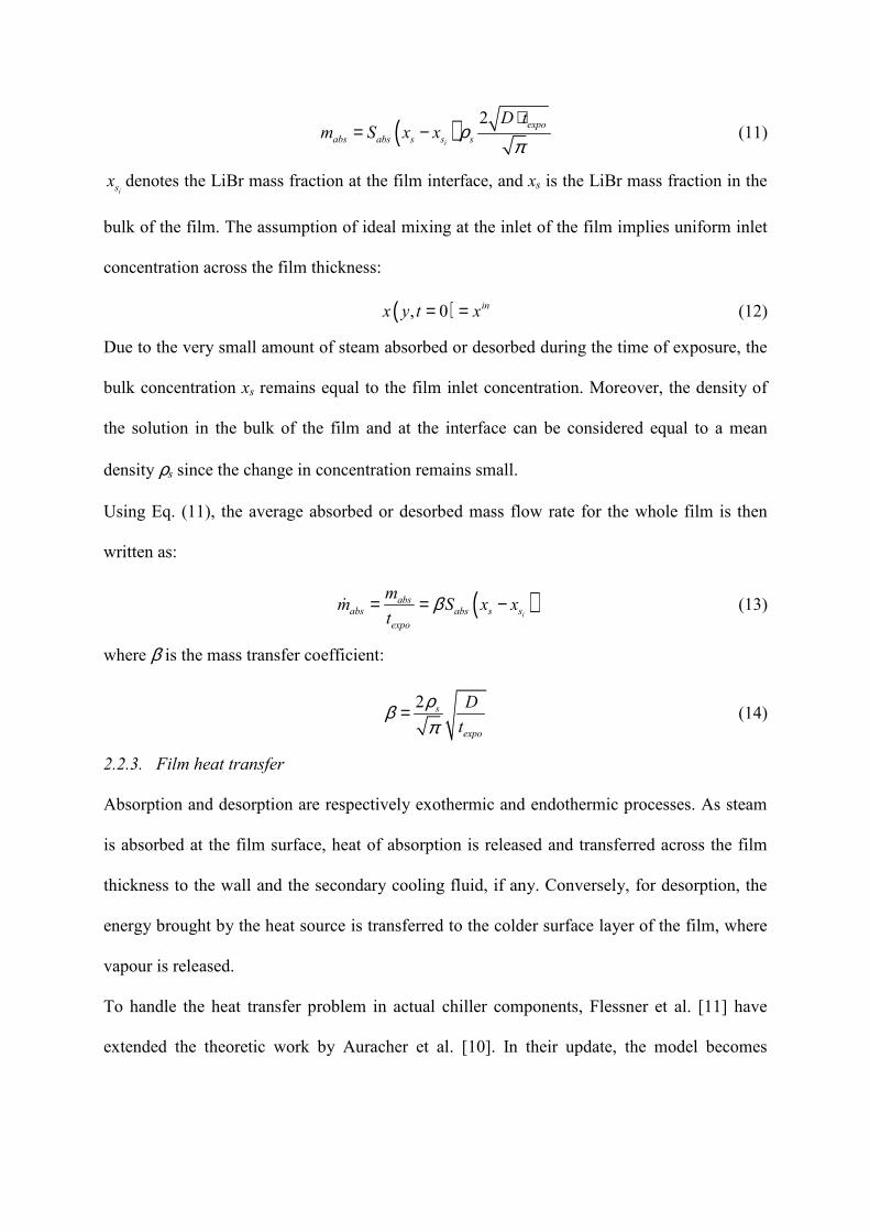
( ) 2

i

expo

abs abs s s s

D tm S x x ρ

π⋅

= − (11)

isx denotes the LiBr mass fraction at the film interface, and xs is the LiBr mass fraction in the

bulk of the film. The assumption of ideal mixing at the inlet of the film implies uniform inlet

concentration across the film thickness:

( ), 0 inx y t x= = (12)

Due to the very small amount of steam absorbed or desorbed during the time of exposure, the

bulk concentration xs remains equal to the film inlet concentration. Moreover, the density of

the solution in the bulk of the film and at the interface can be considered equal to a mean

density ρs since the change in concentration remains small.

Using Eq. (11), the average absorbed or desorbed mass flow rate for the whole film is then

written as:

( )i

absabs abs s s

expo

mm S x x

tβ= = −& (13)

where β is the mass transfer coefficient:

2 s

expo

D

t

ρβπ

= (14)

2.2.3. Film heat transfer

Absorption and desorption are respectively exothermic and endothermic processes. As steam

is absorbed at the film surface, heat of absorption is released and transferred across the film

thickness to the wall and the secondary cooling fluid, if any. Conversely, for desorption, the

energy brought by the heat source is transferred to the colder surface layer of the film, where

vapour is released.

To handle the heat transfer problem in actual chiller components, Flessner et al. [11] have

extended the theoretic work by Auracher et al. [10]. In their update, the model becomes

applicable to subcooled and superheated conditions in the bulk phase of the film. To do so,

the film is divided into two layers:

- the outer layer, in contact with the vapour phase, where the heat transfer between the

film surface and the core is coupled with the mass transfer of the

absorption/desorption process;

- the inner layer, where the heat transfer between the core of the film and the wall is

assumed to be independent of the mass transfer occurring at the surface.

In both layers, the temperature profile is assumed to be linear. However, in the outer layer, the

temperature gradient is steeper than in the inner layer due to the local release/absorption of

latent heat at the film surface. Using Nusselt’s theory, heat transfer is calculated separately in

each layer. The coupling between the two layers is achieved thanks to the interface

temperature Ts (see Figure 2). As a first approximation, Flessner et al. [11] constantly set this

coupling temperature as the mixed cup temperature at the film outlet out

sT , obtained from the

energy balance over the whole film. They also assume a distribution of the overall film

thickness between the two layers as follows:

outer filmaδ δ= (15)

with the value of a set to 0.1. Strictly speaking, this constant should be determined from

experimental data; however, the value used by Flessner et al. [11] in first approximation is

consistent with other works from the literature [14].

Thus, in the outer layer:

( )iabs abs outer abs s sm h S T Tα∆ = −& (16)

with absh∆ the latent heat of absorption and is

T the film surface temperature. It should be

noticed that the coupling between heat and mass transfer is ensured in the model by eq. (16).

In the inner layer, only sensible heat transfer occurs. The heat flux wQ& (W.m-2) exchanged

with the wall reads:

( )w inner abs s wQ S T Tα= −& (17)

with wT the wall temperature. The heat transfer coefficient across each layer (outer and inner)

is:

slayer

layer

kαδ

= (18)

where ks is the thermal conductivity of the solution. Finally, the equilibrium between the

vapour and the liquid phases is assumed to be effective only at the film surface:

( ),i is sT T x p= (19)

where p is the pressure at the film surface.

2.3. Evaporator-absorber

2.3.1. Description

The so-called evaporator-absorber is a custom component, derived from the technology

presented in [15]. It has been specifically designed to integrate in a single unit two essential

functions usually ensured by two distinctive heat exchangers in conventional absorption

chillers:

- the evaporation of liquid refrigerant on the low pressure side (usually ensured by the

evaporator);

- the absorption of gaseous refrigerant by the absorbent solution (usually ensured by the

absorber).

This type of design is necessitated by the important recirculation rate used in this absorption

cycle: only a small fraction of the refrigerant flow is brought to gas phase and absorbed by the

lithium bromide solution. The working principle of the evaporator-absorber is illustrated by

Figure 3. It is basically constituted of an array of vertical parallel plates enclosed in an airtight

chamber. Each plate is fed by a horizontal distribution tube located on its top edge. The wall

of the tube is drilled, in order to generate a falling film on the entire surface of the plate. The

fluid distribution is alternate: refrigerant on the odd plates, strong absorbent solution on the

even plates. Hence, a refrigerant falling film is always facing an absorbent falling film. Due to

the difference between the refrigerant inlet line pressure and the chamber internal pressure, a

fraction of the refrigerant instantly goes into gas phase as soon as it enters the chamber (flash

evaporation). Another minim fraction is then evaporated as the saturated liquid streams down

the plate (slight pressure loss). Saturated refrigerant vapour accumulates in the evaporator-

absorber chamber until it is absorbed at the surface of the facing lithium bromide solution

film. As shown in the falling film modelling section, the absorption rate is dependant on the

solution inlet conditions (temperature, concentration) as well as on the falling film kinematics.

At the bottom of the plates, both fluids drip in a drainage tray, preventing direct mixing of the

liquid phases.

The sizing of the evaporator-absorber (i.e. the number and dimensions of evaporation and

absorption plates) ensures that the thermal power removed from the conditioned volume and

carried by the refrigerant is transferred to the absorbent solution at a sufficient rate. Thus,

through this component, the refrigerant temperature decreases whereas the lithium bromide

solution temperature increases.

2.3.2. Modelling

The modelling approach used for the evaporator-absorber is illustrated by Figure 5. Four

nodes are defined: the refrigerant inlet, the adiabatic chamber, the absorbent solution film and

the absorber plate (or “wall”). Mass, energy and species balances are then written for the

relevant nodes.

On the refrigerant side, only the flash evaporation is taken into account, as it represents the

essential part of the refrigerant phase change. This means that the evaporation caused by

friction pressure loss along the plates is neglected. The mass and energy balance at the

refrigerant inlet read:

EVin EV EVout

flashm m m= +& & & (20)

EVin EVin EV EV EVout EVout

flash flashm h m h m h= +& & (21)

The flashed vapour is saturated vapour and the residual liquid (refrigerant film) leaving the

evaporator-absorber is saturated liquid, corresponding to the internal pressure EVASp :

( )sat

EV EVAS

flash vh h p= (22)

( )sat

EVout EVAS

lh h p= (23)

The adiabatic chamber node is handled as an accumulation node in terms of vapour mass

EVASM and specific internal energy EVASu :

EVAS

EV AS

flash abs

dMm m

dt= −& & (24)

( )EVAS EVAS EV EV AS EVAS

flash flash abs

dM u m h m h

dt= −& & (25)

where EV

absm& is the total mass flow rate of vapour absorbed by the lithium bromide films. EVASh

is the specific enthalpy corresponding to the specific internal energy of the accumulated

vapour. The internal pressure is given by an equation of state:

( ),EVAS EVAS EVASp p u ν= (26)

with EVASν the specific volume of the refrigerant vapour, calculated on the basis of the total

vapour mass present in the chamber (the total free volume being EVASV ):

EVAS

EVAS

EVAS

V

Mν = (27)

For the absorbent film node, the total mass balance (Eq. (28)), the lithium bromide mass

balance (Eq. (29)) and the energy balance (Eq. (30)) are written. No mass storage in the liquid

phase is assumed, but the energy balance is instationary to account for heat storage in the

control volume:

0ASin AS ASout

s abs sm m m+ − =& & & (28)

0ASin ASin ASout ASout

s sm x m x− =& & (29)

AS

ASin ASin ASout ASout AS EVAS ASss s s s abs w

dUm h m h m h Q

dt= − + + && & & (30)

The absorption mass flow rate AS

absm& and the heat flux transferred to the plate AS

wQ& are

calculated according to the film modelling approach developed in section 2.2. In particular,

Eqs. (13), (16) and (17) become:

( )AS AS AS ASin AS

abs abs im S x xβ= −& (31)

( )i

AS AS AS AS ASout

abs abs outer abs s sm h S T Tα∆ = −& (32)

( )AS AS AS ASout AS

w inner abs s wQ S T Tα= −& (33)

with the film surface temperature i

AS

sT being the equilibrium temperature of the LiBr solution

at concentration AS

ix and pressure EVASp .

Finally, an instationary energy balance is also considered for the wall node:

AS AS

w w

AS AS

w w

dT Q

dt M Cp=

&

(34)

where AS

wM is the total mass of absorption plates and AS

wCp is the heat capacity of the material

composing the plates.

2.4. Desorber

2.4.1. Description

The function of the desorber (or generator) is to separate the refrigerant (water) from the

absorbent solution in the regeneration loop. It consists in a cylindrical vertical vessel

containing two concentric vertical coils acting as heat transfer surfaces (Figure 4). After being

pumped through the recovery heat exchanger, the preheated weak solution enters the vessel

and feeds a circular distributor located over the coils. A falling film is thus created on the

walls of the coil tubes, whereas hot water from an auxiliary heat source is circulated inside the

coils. Hence, heat is transferred from the hot water to the absorbent solution film surface,

where steam is desorbed. At the top of the vessel, an outlet port allows steam to be sent to the

condenser.

At the bottom of the vessel, the strong solution outlet port is connected to the pump suction

line. If the outlet flow rate is smaller than the falling film flow rate, absorbent solution

accumulates in the solution sump. The lower portion of the coil is then immersed in the liquid

(section 1), resulting in much lower heat and mass transfer coefficients than in the falling film

mode (section 2). This means that the desorption rate is dependant on the level of liquid DSZ

in the vessel. In order to express the ratio between section 1 and section 2, a dimensionless

liquid level is defined as:

*DS

DS

DS

max

ZZ

Z= (35)

where DS

maxZ is the maximal height of liquid in the vessel.

2.4.2. Modelling

In this component, steam generation is modelled according to three successive processes:

- setting up of equilibrium of the preheated solution at the desorber inlet;

- falling film desorption on the heated coils (section 2);

- desorption from the solution sump at the bottom of the vessel (section 1).

Eight nodes are used to describe the desorber. They are represented on Figure 6 with the

relevant mass and energy fluxes. It is assumed that at the exit of the recovery heat exchanger,

the absorbent solution is not at equilibrium and remains in the liquid phase (subcooled liquid).

As soon as the solution enters the desorber, the equilibrium corresponding to the internal

pressure DSp is reached, and some vapour is separated from the solution. For the solution

inlet node, the total mass balance, LiBr mass balance and energy balance are expressed by

Eqs. (36) to (38):

, , 0DSin DS DS

s s inlet v inletm m m− − =& & & (36)

, 0DSin DSin DS DS

s s inlet inletm x m x− =& & (37)

, , , , 0DSin DSin DS DS DS DS

s s s inlet s inlet v inlet v inletm h m h m h− − =& & & (38)

Again, the falling film desorption on the coils is modelled following the approach presented in

section 2.2. In this specific case, Eqs. (13), (16) and (17) become:

( )( )*

, 1DS DS DS DS DS DS

v film ext inlet im S Z x xβ= − −& (39)

( )( )*

, ,2 ,1DS DS DS DS DS DS

v film abs outer ext i s filmm h S Z T Tα∆ = − −& (40)

( )( )*

,2 ,2 , ,21DS DS DS DS DS DS

w inner ext s film wQ S Z T Tα= − −& (41)

with the film surface temperature DS

iT being the equilibrium temperature of the LiBr solution

at concentration DS

ix and pressure DSp .

In order to minimize the number of differential equations in the chiller global model, the

whole exposed portion of the coil (section 2) is handled as a single node, representing a single

film. Since only energy can be stored in the film, the balance equations read:

, , , 0DS DS DS

s inlet s film v filmm m m− − =& & & (42)

, , 0DS DS DS DS

s inlet inlet s film filmm x m x− =& & (43)

,

, , , , , , ,2

DS

s film DS DS DS DS DS DS DS

s inlet s inlet s film s film v film v film w

dUm h m h m h Q

dt= − − + && & & (44)

On the contrary, in the solution sump, both mass and energy can be stored. The solution is

heated by the immersed section of the coils. Perfect mixing is assumed: the properties of the

solution leaving the desorber by the outlet port are equal to that of the solution sump. The

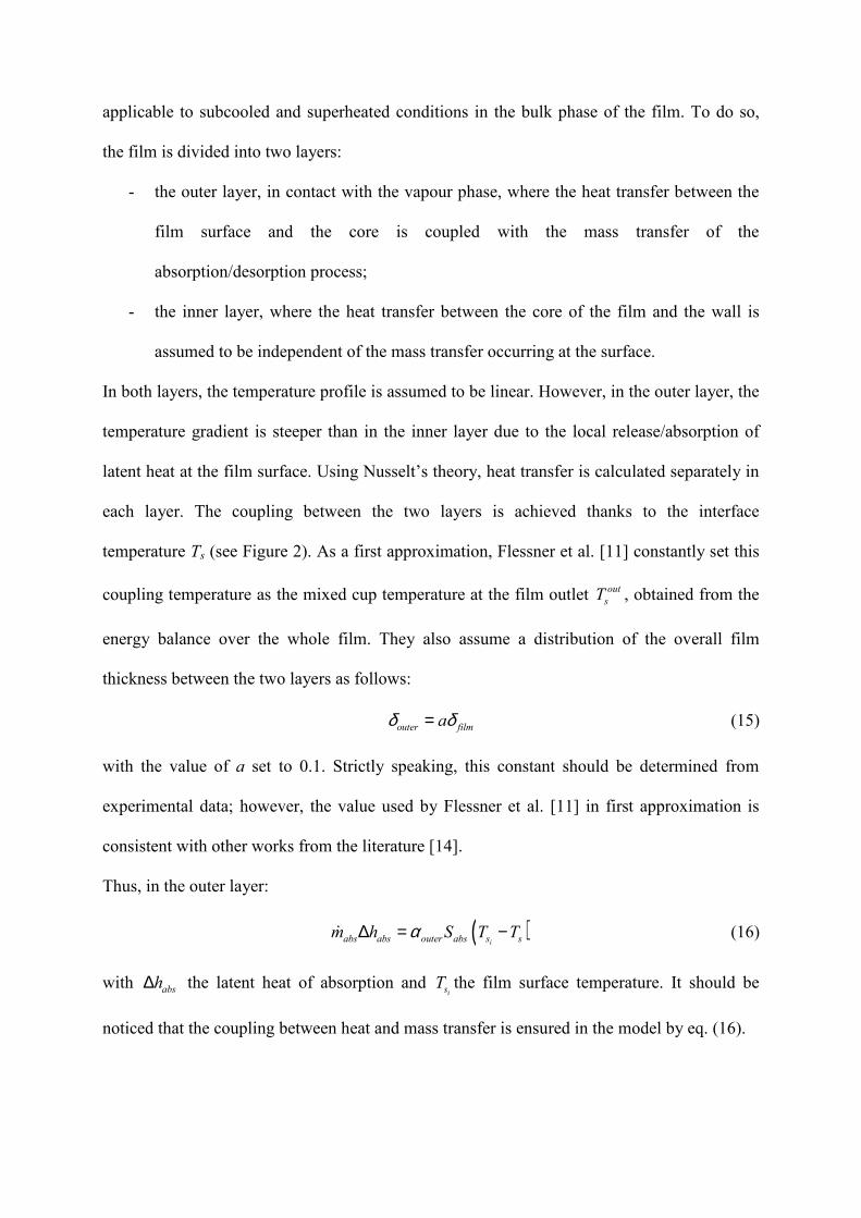
total mass, LiBr mass and energy balances are expressed by Eqs. (45) to (47).

,

, ,

DS

s sump DS DSout DS

s film s v sump

dMm m m

dt= − −& & & (45)

,

,

DS

LiBr sump DS DS DSout DSout

s film film s

dMm x m x

dt= −& & (46)

,

, , , , ,1

DS

s sump DS DS DSout DSout DS DS DS

s film s film s s v sump v sump w

dUm h m h m h Q

dt= − − + && & & (47)

One should note that for all desorption processes, the enthalpy of desorbed vapour is equal to

the enthalpy of super heated vapour at pressure DSp and temperature DSout

ST :

( )DSout

S

DS

v

DS

v Tphh ,= (48)

The overall desorbed vapour flow rate leaving the desorber and sent to the condenser is the

algebraic sum of the individual vapour flow rates generated in the three successive processes:

, , ,

DSout DS DS DS

v v inlet v film v sumpm m m m= + +& & & & (49)

Heat is transferred from the hot water to the LiBr solution through the coil tube. Energy

storage in the walls is taken into account by Eqs. (50) and (51) (respectively section 1 and 2):

( ),1

,1 ,1*

1DS

w DS DS

hw wDS DS DS

w w

dTQ Q

dt M Z Cp= −& & (50)

( ) ( ),2

,2 ,2*

1

1

DS

w DS DS

hw wDS DS DS

w w

dTQ Q

dt M Z Cp= −

−& & (51)

with the heat fluxes on the solution side expressed as:

( )*

,1 ,1 ,1 ,

DS DS DS DS DS DS

w ext ext w s sumpQ S Z T Tα= −& (52)

( ) ( )*

,2 ,2 ,2 ,1DS DS DS DS DS DS

w ext ext w s filmQ S Z T Tα= − −& (53)

Note that in section 2, the external heat transfer between the wall and the solution film is

governed by the heat transfer coefficient of the film inner layer:

,2

DS DS

ext innerα α= (54)

and calculated using Eq. (18).

No energy storage is assumed for the hot water circulating in the coils. The energy balance is

respectively, for section 1 and section 2:

( ), ,1

DS DS DSin DS

hw hw surf hw hwm h h Q− = − && (55)

( ), ,2

DS DSout DS DS

hw hw hw surf hwm h h Q− = − && (56)

The heat fluxes on the hot water side are calculated according to Eqs. (57) and (58):

( )*

,1 int int ,1 ,1

DS DS DS DS DS DS

hw hw wQ S Z T Tα= −& (57)

( )( )*

,2 int int ,2 ,21DS DS DS DS DS DS

hw hw wQ S Z T Tα= − −& (58)

where the water temperatures ,1

DS

hwT and ,2

DS

hwT are the average between the inlet or outlet

temperature ( DSin

hwT or DSout

hwT ) and the hot water temperature at the level of the solution free

surface ,

DS

hw surfT .

2.5. Single phase heat exchangers

In the framework of a complete chiller simulation, true transient distributed models of the heat

exchangers based on finite volume discretization are not suitable because of the high number

of nodes required to simulate complex flow arrangements. In this work, the three single phase

heat exchangers (chilled water HX, solution cooler and heat recovery HX) are modelled using

a pseudo-transient approach. The time-dependant outlet temperature is assumed to follow a

first-order evolution from the initial outlet temperature value 0

outT to the steady-state

temperature value out

stT :

( ) ( )( )0

0

1t

out out out out

stT t T T T t dtτ

= + −∫ (59)

It is important to notice that the steady-state outlet temperature is re-evaluated at each time

step of the simulation. The time constant τ can be determined either experimentally or using

a detailed distributed transient model of the heat exchanger. To do so, the heat exchanger is

simulated independently of the others components, with imposed inlet conditions. Starting

from steady-state, a step in inlet temperature or enthalpy is imposed and the stabilization time

(i.e. the time necessary to reach the new steady-state) is determined. The time constant is

adjusted until the stabilization time in the pseudo-transient model matches that of the detailed

transient model (or the experimental data). As the response is assumed to be of the first order

type, the shape of the pseudo-transient temperature evolution generally differs from the true

transient one. However, the most representative feature of a heat exchanger dynamics is its

time constant, and the use of the pseudo-transient approach leads to sufficiently accurate

results regarding the global chiller dynamics.

The NTU-effectiveness method is used to calculate the steady-state outlet temperatures as

functions of the inlet temperatures, the heat capacity rates of the hot and cold fluid, and the

heat exchanger effectiveness ε :

( ), ,

,h c

out in in inminst h c h c

h c

CT T T T

Cχε= + − (60)

with ( )min ,min h cC C C= , 1χ = for the cold fluid and 1χ = − for the hot fluid. If needed, an

analogous expression using specific enthalpies instead of temperatures for either the hot or the

cold fluid (or even for both fluids) can be derived.

The effectiveness is linked to the number of transfer units (NTU) and the heat capacity rates

by a function f that depends on the configuration of the heat exchanger (see for example [16]):

( ), ,h cf NTU C Cε = (61)

The number of transfer units is defined as the ratio of the overall heat transfer coefficient to

the minimum heat capacity rate:

min

UANTU

C= (62)

The overall heat transfer coefficient takes into account the local heat transfer coefficients and

the heat transfer surfaces on the hot and cold fluid sides, as well as the conduction heat

transfer across the walls:

1

1 1 w

h h c c w w

eUA

S S k Sα α

−

= + +

(63)

The main characteristics of the heat exchangers, including the references of the correlations

used to evaluate the local heat transfer coefficients, are given in tables 1, 2 and 3.

2.6. Condenser

2.6.1. 3-zone model

The pseudo-transient approach used for the single phase heat exchangers is also suitable to

model heat transfer in the condenser. However, in this particular heat exchanger, the

refrigerant is subjected to phase change: it enters as superheated vapour and exits as

subcooled liquid. Therefore, Eqs. (59) and (60) are formulated with enthalpies instead of

temperatures, and the condenser is divided into three distinct sections: the de-superheating

section, the two-phase section and the subcooling section. A fraction of the total heat transfer

area is affected to each section. The refrigerant is treated as a homogeneous fluid. The main

characteristics of the condenser are summarized in table 4.

The distribution of the section areas is not known beforehand, but the state of the fluid at the

section boundaries does. The refrigerant generally enters the condenser in the superheated

vapour state, with a known specific enthalpy. The de-superheating section being defined as

the area necessary for the refrigerant to reach the saturated vapour state, the enthalpy

reduction associated to this section is known. This allows determining successively the

corresponding effectiveness, NTU and heat transfer area necessary to achieve this enthalpy

reduction, according to the method presented in section 2.5. The same methodology is applied

for the determination of the two-phase section heat transfer area, knowing that the refrigerant

enters this section at saturated vapour state and exits at saturated liquid state. Finally, the

subcooling section area can be calculated as the difference between the total heat transfer area

and the sum of the two previous section areas. The corresponding NTU and effectiveness are

then determined, which yields the outlet enthalpy of the condensate.

If the total available heat transfer area is too small to ensure that the refrigerant reaches the

saturated liquid state, the condenser outlet state is two-phase and there is no subcooling

section. The outlet vapour quality of the refrigerant is then evaluated as a function of the

outlet enthalpy and condensation pressure.

2.6.2. Condensation pressure

The pressure at the condenser is assumed to be determined by the pressure in the refrigerant

bottle receiving the condensate. Mass and internal energy storage in the bottle are described

by transient balance equations, and the equilibrium condition (saturated liquid state in the

bottle) yields the bottle pressure.

2.6.3. Condensation heat transfer coefficient

Due to the low refrigerant mass flow rate in the condenser copper tubes, the maximum

Reynolds number of the condensate flow is approximately 15. Using the Nusselt laminar film

analysis, the thickness of the corresponding refrigerant film inside the tubes would be inferior

to 35 µm. Moreover, the wettability of copper is rather low. Consequently, dropwise

condensation is the most likely to occur. Griffith [19] has proposed the following correlation

to estimate the heat transfer coefficient dwcα in dropwise condensation (unit: kW.m-2.K

-1):

51.1 2.04dwc satTα = + (64)

This relationship is valid for 22°C < Tsat < 100 °C.

2.7. Numerical implementation

The equation solver EES has been used to handle the resulting global model. To set up the

global chiller model, all the individual component sets of equations have been linked together

using internal variables, and the initial and external conditions have been specified. The fluid

properties (water and lithium-bromide solution) are available in libraries included in the EES

software. The results presented in this paper have been obtained using a constant simulation

time step of 1 s.

3. APPLICATION

The model consistency and dynamic behaviour can be analyzed by applying a step change to

one of the external parameters, which are of three kinds: the hot water inlet parameters (heat

recovery), the outside air parameters (ambient conditions), and the chilled water inlet

parameters (thermal load).

First, the simulation is started using the input parameters summarized in table 5. The steady

state corresponding to these input parameters is reached after approximately 300 s. It should

be noticed that the choice of the initial values (for differential equations) is arbitrary and has

no effect on the steady state. Then, at t = 500 s, a step change on one of the external control

parameters is imposed, while all the other parameters remain unmodified. The system reacts

to this parameter change and a new steady state is reached after a transient period.

3.1. Response to a reduction of the hot water flow rate in the heat recovery HX

This case is intended to simulate a drop in heat recovery fluid flow rate, which occurs

frequently when the hot fluid circulation pump is directly coupled to a variable speed engine

as, for example, in internal combustion engines. Here, the initial flow rate HR

hwm& is reduced at t

= 500 s from 0.5 kg/s to 0.17 kg/s (approximately divided by 3).

Since less energy is brought to the heat recovery HX, the enthalpy of the absorbent solution

leaving this exchanger instantly decreases (Figure 7a) and the vapour flow rate generated as

the solution enters the desorber decreases as well (Figure 7d) (“desorber inlet” node). This is

also noticeable on the concentration diagram (Figure 7e), where the gap between the recovery

HX concentration and the desorber inlet concentration starts to reduce. As a consequence, the

total vapour flow rate leaving the desorber and sent to the condenser firstly drops, and the

concentration of the strong regenerated solution is reduced, since less refrigerant is extracted.

The regenerated solution then returns to the solution pump suction, where it mixes with the

recirculation loop solution, inducing a general decrease of the concentrations and solution

enthalpies in the chiller. The concentration reduction of the solution leads to a decrease of its

absorption potential. Therefore, in the evaporator-absorber, the vapour flow rate from the

refrigerant to the solution starts to decline (Figure 7d), and so does the heat flux (Figure 7h).

This corresponds to a reduction in the frigorific effect: the enthalpy and the temperature of the

refrigerant leaving the evaporator-absorber and entering the chilled water HX increase (Figure

7b and Figure 7g), leading to a rise of the chilled water temperature and a decrease in the

chilled water HX heat flux representing the frigorific power of the system (Figure 7i).

Since less vapour is desorbed, the thermal load of the condenser is reduced. Therefore, the

degree of subcooling of the condensate increases, so its enthalpy (Figure 7b) and its

temperature (Figure 7f) fall dramatically. In the condensate bottle, this temperature drop is

noticeable, though very attenuated by the damping effect of the stored refrigerant mass. The

liquid-vapour equilibrium in the condensate bottle is therefore modified, and the equilibrium

pressure is lowered. Since in our model, the condensation pressure and the desorber internal

pressure are directly linked to the condensate bottle pressure and vary alike, the liquid-vapour

equilibrium in the desorber is also modified (Figure 7c). Indeed, a reduction of the desorber

pressure level induces a reduction of the refrigerant evaporation temperature, which leads to

an enhancement of the desorption process. This is obvious on Figure 7d: the vapour flow rates

from the desorber film and sump start to increase. On Figure 7e, this results in an increase in

the gap between the desorber inlet and outlet concentrations. As a result, the decreasing total

vapour mass flow rate produced by the desorber and sent to the condenser reaches a

minimum, then starts to re-increase and stabilizes at its steady-state value as the new liquid-

vapour equilibrium is set in the desorber (Figure 7d). The condenser response follows a

similar evolution: since the refrigerant vapour flow rate (i.e. the thermal duty of the

exchanger) re-increases, the degree of subcooling of the refrigerant decreases and its outlet

temperature and enthalpy rise again.

Basically, the evaporator-absorber and the desorber-condenser ensemble behave like self-

regulated systems: if the vapour production is enhanced, their internal pressure increases,

which tends to shift the liquid-vapour equilibrium in a way that penalizes and stabilizes the

desorption rate. Conversely, if the desorption rate decreases, the internal pressure of the

vessels falls and the new equilibrium tends to promote vapour production.

In the present example, the desorption pressure reduction allows the desorber to partially

compensate the power drop in the recovery heat exchanger by an increase in the film and

sump desorption rates. Indeed, this effect is accompanied by an increasing heat flux from the

auxiliary hot water circuit to the absorbent solution through the desorber coil (at constant

auxiliary hot water flow rate and inlet temperature). From the initial steady state to the new

steady state, the heat recovery flux drops from 20.6 to 15.8 kW (-4.8 kW) whereas the

desorber heat flux rises from 13.1 to 15.3 kW (+2.2 kW). Thus, the total heat supply reduces

from 33.6 to 31.1 kW (-2.6 kW) and the frigorific power decreases from 14.2 to 13.0 kW (-

1.2 kW). Eventually, this results in an outlet chilled water warming of barely +0.5°C (9.6 to

10.1 °C).

In terms of dynamic behaviour, the time necessary for the system to reach the new steady

state after the heat recovery flow rate change is approximately 100 s. This time is likely to be

underestimated, as no transport delays have been included in the model: as a first

approximation, the time needed for the solution and refrigerant to convey any state changes

through the circuit has not been taken into account. However, the emphasis has been put on

modelling the physical phenomena occurring in the falling film based components (i.e. the

evaporator-absorber and the desorber), whereas the dynamics of the other heat exchangers

have been implemented rather coarsely.

3.2. Response to a reduction of the chilled water inlet temperature

This case attempts to simulate the chiller response to a sudden reduction of cooling demand of

the conditioned space air. Indeed, the heat flux entering the chilled water in the air handling

units drops, inducing a decrease in its temperature as it is sent back to the chiller. It is clear

that the step change represents an extreme solicitation unlikely to occur in normal operation

conditions. However, as the aim of this simulation is to highlight the trends of the dynamic

behaviour of the system, a simple and instantaneous perturbation have been chosen. In

opposition to the previous simulation case, the system is thermostated: the hot water flow rate

powering the main recovery heat exchanger is kept constant, but the hot water flow rate

supplying energy to the desorber (auxiliary circuit) is controlled according to the chilled water

outlet temperature:

( ):

:

:

CWout DS

cw min hw min

CWout DS CWoutmax minmin cw max hw min cw min

max min

CWout DS

cw max hw max

T T m m

m mT T T m m T T

T T

T T m m

< =

−≤ ≤ = + − −

> =

& &

& && &

& &

(65)

Between the temperature thresholds Tmin and Tmax, the hot water flow rate (i.e. the thermostat

opening) is a linear function of the chilled water outlet temperature. The minimal and

maximal values of the hot water flow rate are respectively 0.001 kg/s and 0.5 kg/s. Those of

the chilled water outlet temperature are respectively 9.5°C and 10.5°C.

The evolution of some internal variables is shown on Figure 8. The initial chilled water inlet

temperature is set at 16 °C and all the other input parameters are those of table 5. With these

parameters, the chilled water outlet temperature stabilizes at 10.45 °C, i.e. slightly below the

upper threshold of the thermostat, and the corresponding auxiliary hot water flow rate is 0.48

kg/s. The generated frigorific power is then 14.8 kW. For the initial conditions, the mass and

heat transfer coefficients in the lithium bromide film are equal to 0.15 kg.m-2.s

-1 and

1980 W.m-2.K

-1 respectively.

The steady state being reached, at t = 500 s, the chilled water inlet temperature is lowered to

13 °C (Figure 8a). As a result, the chilled water outlet temperature instantly falls under the

thermostat lower threshold (down to 9°C), resulting in a drop of the desorber hot water flow

rate to the minimal value (Figure 8b). Consequently, the vapour flow rate generated thanks to

the desorber coils (i.e. film desorption and sump desorption) drops as well. The desorber heat

flux falls from 14 kW to 1.7 kW. The overall desorbed vapour flow rate being balanced by the

absorbed vapour flow rate, the evaporator-absorber heat flux also drops.

Since the overall vapour flow rate decreases, the refrigerant condensation heat flux (Figure 8f)

and temperature decrease, and the desorption pressure (related to the condensation pressure)

declines (Figure 8d). Thus, because of the new liquid-vapour equilibrium in the desorber, the

desorption potential of the preheated solution is enhanced: at the desorber inlet, the vapour

flow rate caused by the preheating of the solution in the recovery heat exchanger starts to

increase (Figure 8c). Moreover, the desorption temperature is lowered and the strong solution

leaving the desorber and returning to the circuit becomes colder: as a result, the heat flux in

the heat recovery HX increases and the heat flux in the solution cooler decreases (Figure 8f).

The hot water flow rate in the desorber coil remains at its minimal value for about 10 s,

allowing the chilled water temperature to re-increase over the lower limit and the thermostat

to re-open. The thermostat opening then starts to oscillate in a damped way with the chilled

water temperature, until the latter eventually stabilizes at the lower limit of 9.5 °C. The

oscillation period is approximately 12 s. The observed physical oscillations are linked to the

choice of the temperature control. Another type of regulation could result in lower

oscillations. It can be noticed that all the variables represented on Figure 8 show oscillations,

except the pressure. Indeed, the desorber internal pressure is governed by the internal pressure

of the condensate bottle, itself determined by the temperature of the stored condensate.

Reminding that perfect mixing is assumed for all mass storages, the refrigerant temperature in

the bottle is practically not sensitive to the oscillations of the incoming condensate

temperature. Moreover, the time needed to stabilize the bottle temperature affects the

desorption pressure evolution, and consequently, the evolution of the desorption rates. This

time obviously depends on the amount of refrigerant stored in the bottle. In the present

simulation, the bottle is filled with nearly 2 kg, and the desorption pressure reaches steady

state after approximately 300 s.

4. CONCLUSION

In this paper, a model able to simulate the dynamic behaviour of a special absorption chiller is

presented. In the desorber and the evaporator-absorber, the lithium bromide solution falling

films are described in a lumped manner by a simple physical approach based on Nusselt’s

theory. As opposed to a standard approach based on empirical parameters, this formulation

links the absorption/desorption rates to the film geometrical characteristics, i.e. to the design

parameters of the heat transfer surfaces. Transient balances accounting for mass and heat

storage are considered for both components. Other heat exchangers are modelled according to

the NUT-effectiveness method coupled with a time constant. The resulting global model is

used to investigate the dynamic response of the chiller to external conditions variations: step

change in the hot water flow rate sent to the main recovery heat exchanger, and step change in

the inlet temperature of the chilled water, (i.e. a drop of the chiller thermal load). A simple

temperature regulation law has been implemented in the latter case. Both studied cases show

that the model is able to simulate the detailed performance of the chiller with good

consistency. The response of the system to basic input parameters changes appears to be

qualitatively realistic, even if the time constants are probably underestimated since the

transport delays of the solutions through the piping have not been taken into account.

However, the detailed physical modelling of the falling film enables a clear understanding of

the desorber and evaporator-absorber responses to various condition changes, and in

particular, their self-regulated behaviour linked to the control of the condensation and

evaporation pressures. Next steps of this work include model validation against experimental

measurements and implementation of more accurate dynamics for solution transport and heat

exchangers transient responses.

Acknowledgements

This work was made within the framework of a French project of the cluster Lyon Urban

Truck and Bus named “CLIMAIRIS” supported by the General Directorate for Enterprise

(DGE).

References

[1] Z.F. Li, K. Sumathy, Simulation of a solar absorption air conditioning system, Energy

Convers. Manag. 42 (2001) 313-327.

[2] H. Liu, K.E. N’Tsoukpoe, N. Le Pierres, L. Luo, Evaluation of a seasonal storage system

of solar energy for house heating using different absorption couples, Energy Convers. Manag.

52 (2011) 2427-2436.

[3] K.A. Joudi, A.H. Lafta, Simulation of a simple absorption refrigeration system, Energy

Convers. Manag. 42 (2001) 1575-1605.

[4] S. Jeong, B.H. Kang, S.W. Karng, Dynamic simulation of an absorption heat pump for

recovering low grade waste heat, Appl. Therm. Eng. 18 (1998) 1-12.

[5] D.G. Fu, G. Poncia, Z. Lu, Implementation of an object-oriented dynamic modeling

library for absorption refrigeration systems, Appl. Therm. Eng. 26 (2006) 217-225.

[6] P. Kohlenbach, F. Ziegler, A dynamic simulation model for transient absorption chiller

performance. Part I: The model, Int. J. Refrigeration 31 (2008) 217-225.

[7] P. Kohlenbach, F. Ziegler, A dynamic simulation model for transient absorption chiller

performance. Part II: Numerical results and experimental verification, Int. J. Refrigeration 31

(2008) 226-233.

[8] H. Matsushima, T. Fujii, T. Komatsu, A. Nishiguchi, Dynamic simulation program with

object-oriented formulation for absorption chillers (modelling, verification, and application to

triple-effect absorption chiller), Int. J. Refrigeration 33 (2010) 259-268.

[9] B. Bakhtiari, L. Fradette, R. Legros, J. Paris, A model for analysis and design of H2O-LiBr

absorption heat pumps, Energy Convers. Manag. 52 (2011) 1439-1448.

[10] H. Auracher, A. Wohlfeil, F. Ziegler, A simple model for steam absorption into a falling

film of aqueous lithium bromide solution on a horizontal tube, Heat Mass Transfer 44 (2008)

1529-1536.

[11] C. Flessner, S. Petersen, F. Ziegler, Simulation of an absorption chiller based on a

physical model, Proceedings of the 7th Modelica Conference, Como, Italy, 2009, pp. 312-317.

[12] J.D. Killion, S. Garimella, A critical review of models of coupled heat and mass transfer

in falling-film absorption, Int. J. Refrigeration 24 (2001) 755-797.

[13] G. Grossman, Heat and mass transfer in film absorption, in: Cheremisinoff, N.P. (Ed.),

Handbook of Heat and Mass Transfer, Vol. 2. Gulf Publishing Co., Houston, 1986, pp. 211-

257.

[14] S. Jeong, S. Garimella, Falling-film and droplet mode heat and mass transfer in a

horizontal tube LiBr/water absorber, Int. J. Heat Mass Transfer 45 (2002) 1445-1458.

[15] E. Boudard, V. Bruzzo, Heat exchange and heat transfer device, in particular for a motor

vehicle, European Patent 1751477B1 (2009).

[16] R.K. Shah, A.C. Mueller, Heat exchangers, in: Rohsenow, W.M., Hartnett, J.P., Ganic,

E.N. (Eds.), Handbook of Heat Transfer Applications, 2nd

Edition. McGraw-Hill, New York,

1985, pp. 4.1-4.312.

[17] H. Kumar, The plate heat exchanger: construction and design, 1st UK National

Conference on Heat Transfer, University of Leeds, Inst. Chem. Symp, United Kingdom, 1984,

Series 86, pp. 1275-1286.

[18] C.C. Wang, C.J. Lee, C.T. Chang, S.P. Lin, Heat transfer and friction correlation for

compact louvered fin-and-tube heat exchangers, Int. J. Heat Mass Transfer 42 (1999) 1945-

1956.

[19] P. Griffith, Dropwise condensation, in: Schlunder, E.U., (Ed.), Heat Exchanger Design

Handbook, Vol. 2, Hemisphere Publishing, New York, 1983.

[20] C.C. Wang, K.Y. Chi, C.J. Chang, Heat transfer and friction characteristics of plain fin-

and-tube heat exchangers, part II : Correlation, Int. J. Heat Mass Transfer 43 (2000) 2693-

2700.

Figure 1 – Diagram of the complete chiller

Figure 2 - Schematic of a modelled falling film, showing the temperature and LiBr

concentration profiles. a) Absorption; b) Desorption

Figure 3 - Working principle of the evaporator-absorber

Figure 4 - Working principle of the desorber

Figure 5 - Equivalent model diagram of the evaporator-absorber

Figure 6 - Equivalent model diagram of the desorber

Figure 7 - Simulated chiller response on a heat recovery water flow rate reduction (0.5 kg/s to

0.17 kg/s), without regulation

Figure 8 - Simulated chiller response on a chilled water inlet temperature change (16°C to

13°C), with regulated chiller water outlet temperature (min: 9.5°C, max: 10.5°C)

TABLE 1 - Chilled water heat exchanger characteristics

Feature Unit Hot Fluid Side Cold fluid side

Type - Welded plates

Configuration - 15 parallel plates

Fluid - Ethylene glycol Water (refrigerant)

Flow arrangement - 1 pass, counterflow 1 pass, counterflow

Mass flow rate kg.s-1 0.72 0.90

Capacity rate kW.K-1 2.7 3.8

H.T. surface m² 1.5 1.5

H.T. coefficient kW.m-2.K

-1 4.4 7.9

H.T. coeff. correlation ref. - Kumar [17] Kumar [17]

Overall H.T. coefficient kW.m-2.K

-1 4.2

Number of transfer units - 1.6

Effectiveness - 0.67

Time constant s 1.75

TABLE 2 - Absorbent solution cooler characteristics


Type - Forced convection louvered fin-and-tube

Configuration - 66 parallel coils

Fluid - LiBr solution Air

Flow arrangement - 6 passes, crossflow 1 pass, crossflow

Air velocity m.s-1 - 2.5

Mass flow rate kg.s-1 3.0 -


H.T. surface m² 38 458


-1 1.7 0.099

H.T. coeff. correlation ref. - Dittus-Boelter Wang et al. [18]


-1 26.6



Time constant s 3.5

TABLE 3 - Heat recovery heat exchanger characteristics


Type - Welded plates

Configuration - 33 parallel plates

Fluid - Ethylene glycol LiBr solution

Flow arrangement - 1 pass 16 passes

Mass flow rate kg.s-1 0.50 0.20


H.T. surface m² 0.53 0.53


-1 10.2 1.79

H.T. coeff. correlation ref. - Kumar [17] Kumar [17]


-1 0.8



Time constant s 3

TABLE 4 – Condenser characteristics


Type - Forced convection plain fin-and-tube

Configuration - 2 rows of 60 parallel tubes

Fluid - Water (refrigerant) Air

Flow arrangement - 1 pass, crossflow 1 pass, crossflow

Air velocity m.s-1 - 2.5

Mass flow rate kg.s-1 0.005 -

Capacity rate kW.K-1 ∞ 2.5

H.T. surface m² 1.2 34


-1 131 0.078

H.T. coeff. correlation ref. - Griffith [19] Wang et al. [20]


-1 2.6

Number of transfer units - de-superheating: 2.9 - 2-phase: 1.1 - subcooling: ≈ 0

Effectiveness - de-superheating: 0.83 - 2-phase: 0.65 - subcooling: ≈ 0

Time constant s 5

TABLE 5 - Initial steady-state input parameters

Parameter Symbol Unit Value

Chilled water inlet temperature CWin

cwT °C 15

Chilled water mass flow rate CW

cwm& kg.s

-1 0.72

Outside air temperature airT °C 30

Outside air velocity airv m.s

-1 2.5

Heat recovery HX hot water inlet temperature HRin

hwT °C 105

Heat recovery HX hot water mass flow rate HR

hwm& kg.s

-1 0.5

Desorber hot water inlet temperature DSin

hwT °C 110

Desorber hot water mass flow rate DS

hwm& kg.s

-1 0.4

Refrigerant pump mass flow rate (chilled water HX inlet) CWm& kg.s

-1 0.9

Regeneration loop mass flow rate (heat recovery HX inlet) HRm& kg.s

-1 0.2

Recirculation loop mass flow rate (solution cooler inlet) SCm& kg.s

-1 3.0

Documents

A numerical model for the dynamic simulation of a