A numerical method to calculate Nash-Cournot equilibria in

electricity markets

Javier Contreras Jacek B. KrawczykUCLM Victoria University of WellingtonCiudad Real WellingtonSpain New Zealand

2

Summaryn Introductionn Definitions and conceptsn The relaxation algorithmn Duopoly examplen Case study 1n Case study 2n Conclusions

3

Introductionn Power system restructuring fosters

competitionn Cost minimization schemes replaced by

bidding algorithmsn Nash Equilibria in network-constrained

electricity markets

4

Introductionn Nikaido-Isoda Relaxation Algorithm

(NIRA)n Convergence to a Nash-Cournot

equilibriumn Unique solution under certain conditionsn NIRA solves coupled constraint gamesn Applicable to electricity markets

5

Definitions and conceptsn A game represents:

– a set of individuals interacting – strategic interdependence

n To describe a game you need:– players– rules of the game– outcomes– payoffs

6

Definitions and conceptsn Information set: information about his

own and other players’ actions. It constains information on what is observable

n Strategy: A rule that tells the player wich action he should take, according to his information set

n Action: a choice made by a player as a result of his strategy

7

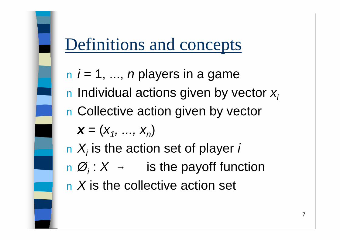
Definitions and conceptsn i = 1, ..., n players in a gamen Individual actions given by vector xi

n Collective action given by vector x = (x1, ..., xn)

n Xi is the action set of player in Øi : X is the payoff functionn X is the collective action set

→ ℜ

8

Definitions and conceptsn x = (x1, ..., xn) and y = (y1, ..., yn) are

elements of the collective action set Xn An element

of X is a set of actions where the ith player plays yi while the remaining agents play xj

n A point x* = (x1*, ..., xn

*) is called the Nash equilibrium point if, for each i,

( ) ),,,,,,(| 111 niiii xxyxxy LL +−≡x

)(max)()(

xx*x

*ii

Xxi x

i

φφ∈

=|

9

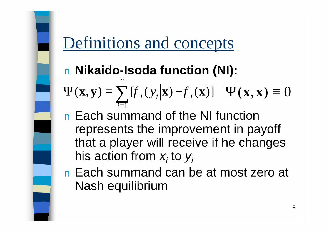
Definitions and conceptsn Nikaido-Isoda function (NI):

n Each summand of the NI function represents the improvement in payoff that a player will receive if he changes his action from xi to yi

n Each summand can be at most zero at Nash equilibrium

])()([),(1

∑=

−=Ψn

iiii y xxyx φφ 0),( ≡Ψ xx

10

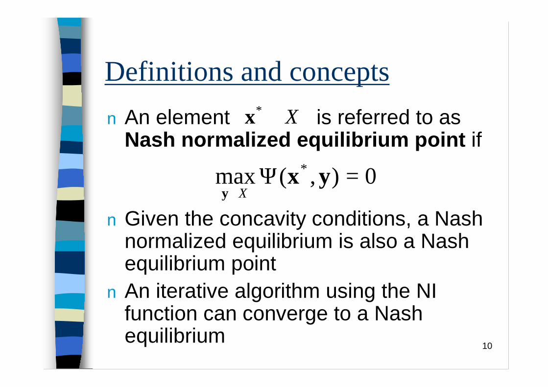
Definitions and conceptsn An element is referred to as

Nash normalized equilibrium point if

n Given the concavity conditions, a Nash normalized equilibrium is also a Nash equilibrium point

n An iterative algorithm using the NI function can converge to a Nash equilibrium

X∈*x

0),(max * =Ψ∈

yxy X

11

Definitions and conceptsn The optimum response function at

the point x is

n All players try to unilaterally maximize their payoffs

n By playing actions Z(x), rather than x, the players approach the equilibrium

XZZX

∈Ψ=∈

)( , ),,(max arg)( xxyxxy

12

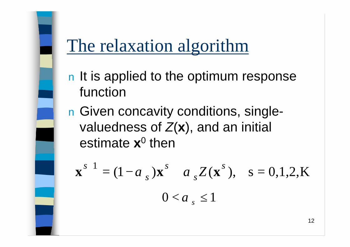
The relaxation algorithmn It is applied to the optimum response

functionn Given concavity conditions, single-

valuedness of Z(x), and an initial estimate x0 then

K0,1,2,s ),()1(1 =+−=+ ss

ss

s Z xxx αα

10 ≤< sα

13

The relaxation algorithmn An iterative step s+1 is constructed as a

weighted average of the improvement point Z(xs) and the current point xs

n The optimum response function Z(xs) is a result of maximizing the NI function

n The averaging ensures convergence of the algorithm under certain conditions

14

The relaxation algorithmn Taking a sufficient number of iterations

the NIRA converges to the Nash equilibrium x*

n The problem calculates the successive actions taken by the players at each stage when optimizing their response unilaterally

15

The relaxation algorithmn To ensure convergence of NIRA, the most

important condition in coupled constraint games is Diagonal Strict Concavity (DSC)

n DSC means that each player has more control over his payoff than the other players have over it

n Coupled constraint games can be due, for example, to Kirchhoff’s laws

16

Duopoly examplen Two identical firms selling a productnMarket price:n Profit made by firm i:

n The Nikaido-Isoda function :

)()( 21 xxp +−= ραx

iiii xxxxxp ])([)()( 21 +−−=−= ρλαλφ xx

221221

121121

])([])([ ])([])([xxxyyxxxxyxy

+−−−+−−++−−−+−−

ρλαρλαρλαρλα

),( yxΨ

17

Duopoly examplen The optimum response function Z(x):

),(21)1 ,1(

2),(max arg 12 xx

X−

−=Ψ

∈ ρλαyx

y

22 ;

22

e wher),,(),(

12

21

2121

xyxy

yyxxZ

−−

=−−

=

=

ρλα

ρλα

18

Duopoly examplen Convergence to Nash equilibrium if:

is positive definite

xyyyxyxxQ == Ψ−Ψ= ),(),(),( yxyxxx

19

Duopoly example

2112

2ρ =

xy

yy

yy

xy

xx

xx

xyyyxyxx

yyxxy

yyxxy

yyxxy

yyxxy

yyxxx

yyxxx

yyxxx

yyxxx

Q

=

=

==

Ψ∂∂

Ψ∂∂

Ψ∂∂

Ψ∂∂

−

Ψ∂∂

Ψ∂∂

Ψ∂∂

Ψ∂∂

=Ψ−Ψ=

),,,(),,,(

),,,(),,,(

),,,(),,,(

),,,(),,,(

),(),(),(

212122

212121

212112

212111

212122

212121

212112

212111

yxyxxx

20

Case study 1n Three-bus systemn Unlimited capacity generators at buses

1 and 2n Demand at buses 1, 2 and 3n Each pair of buses connected by a

transmission linen No transmission line flow limits

21

Case study 1n Demand functions:

pi(qi) = 40 – 0.08*qi for buses i = 1, 2p3(q3) = 32 – 0.0516*q3 for bus 3

n Generator constant marginal costs are $15/MWh and $20/MWh, respectively

n Bilateral market: sij means that generator (company) i sells s MW to consumers at node j

n Pfgi is the production of generator g of company f placed at node i

22

Case study 1n Each generator (company) maximizes profit:

sales revenue – generation cost

subject to

fgigi

fgifjfk

kjfjjojoj

jo PPCsssQPP ∑∑∑ −+−≠ ,

)(]))(/([max

0

generators , nodes ,

,

,

max

≥∀

=

=

∀≤

∑

∑∑

fgifj

jf

fj

gifgi

jfj

fgifgi

Ps

qs

Ps

giPP

23

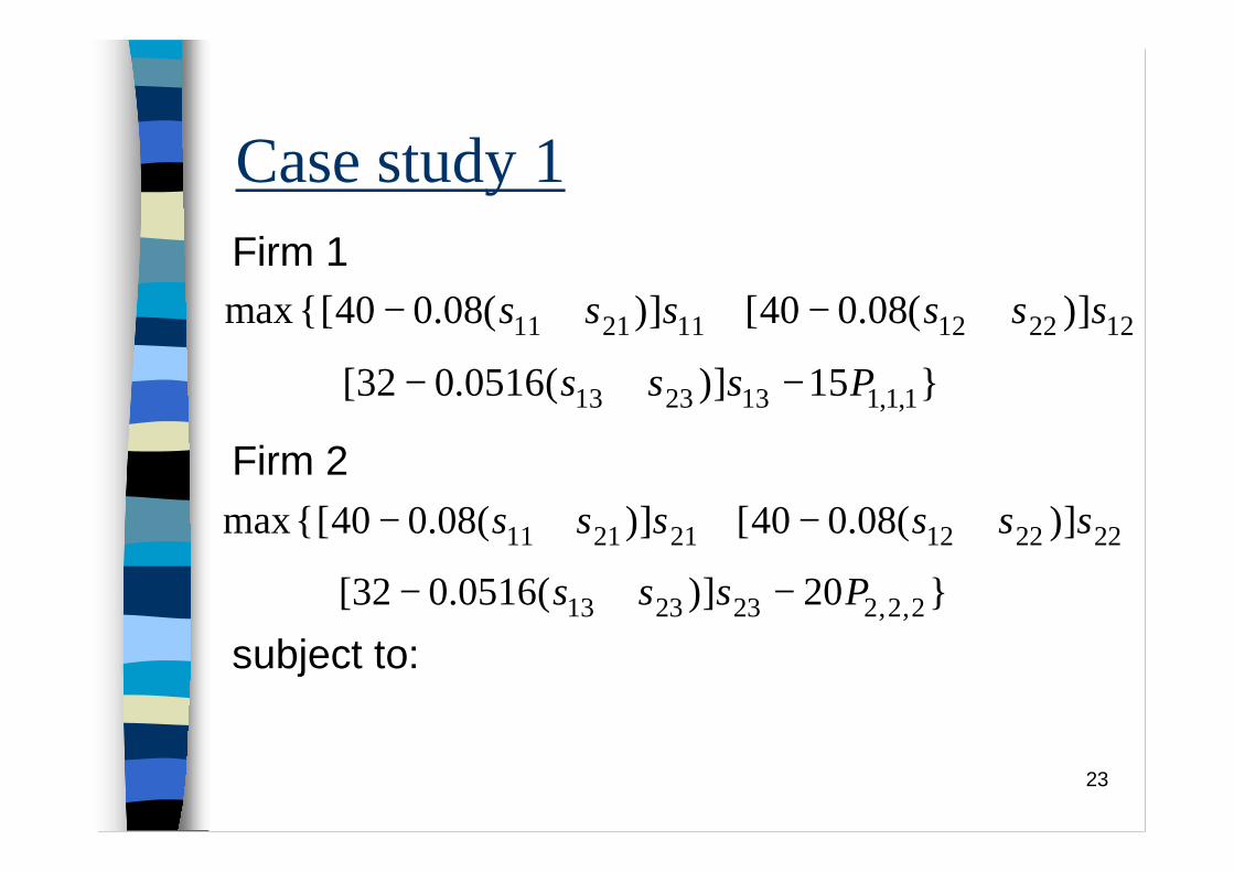
Case study 1Firm 1

Firm 2

subject to:

}15])(0516.032[

])(08.040[])(08.040[ { max

1,1,1132313

122212112111

Psss

ssssss

−+−+

+−++−

}20])(0516.032[

])(08.040[])(08.040[ { max

2,2,2232313

222212212111

Psss

ssssss

−+−+

+−++−

24

Case study 1

0,,,,,

,)()(

,)()(

,)()(

,,,

,,

232221131211

323

32

13

31

223

23

12

212,2,2

113

13

12

121,1,1

23133

22122

21111

2322212,2,2

1312111,1,1

≥

=−

+−

=−

+−

+

=−

+−

+

+=+=+=

++=

++=

ssssss

qx

Sx

S

qx

Sx

SP

qx

Sx

SP

ssqssqssq

sssPsssP

basebase

basebase

basebase

θθθθ

θθθθ

θθθθ

25

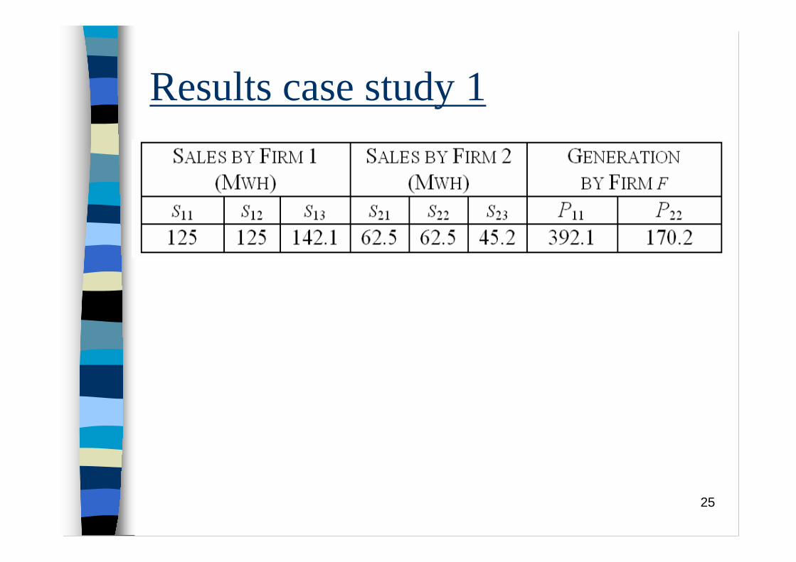
Results case study 1

26

Results case study 1

n q1 = 187.5 MW, price1 = $25/MWh n q2 = 187.5 MW, price2 = $25/MWh n q3 = 187.3 MW, price3 = $22.3/MWhn Flow 1-2: 73.95 MWn Flow 1-3: 130.65 MWn Flow 2-3: 56.7 MWn Profit1 = $/h 3542.1n Profit2 = $/h 730.6

27

Case study 2n Transmission line flow limit of 25 MW on

line 1-2 (binding constraint)n New constraints added to the ones in

case study 1:

baseSx25

12

21 ≤−θθ baseSx

25

12

21 ≤−θθ

baseSx25

12

12 ≤−θθ

28

Results case study 2

29

Results case study 2

30

Results case study 2

n q1 = 199.1 MW, price1 = $24.1/MWh n q2 = 175.9 MW, price2 = $25.9/MWh n q3 = 187.3 MW, price3 = $22.3/MWhn Flow 1-2: 25 MWn Flow 1-3: 106.15 MWn Flow 2-3: 81.15 MWn Profit1 = $/h 2985n Profit2 = $/h 956.9

31

Case study 2: constraint enforcementn Assume an authority is empowered to

charge agents from deviations of the line flow limit

n The Lagrange multipliers of the activeconstraints (Kirchhoff’s law and line flow limits) calculated by NIRA can be used to enforce constraints

32

Case study 2: constraint enforcementn The Lagrange multipliers decouple a

game where the players’ actions are coupled through constraints

n The steps of the procedure are as follows:

33

Case study 2: constraint enforcement1. The regulator solves a coupled constraint

game, i.e. computes production levels (which do not violate constraints) and the Lagrange multipliers

2. The regulator modifies the players’ payoffs by telling them the value of the Lagrange multipliers

3. The players solve the new game with new payoffs and “miraculously” obtain the same production levels as the regulator

34

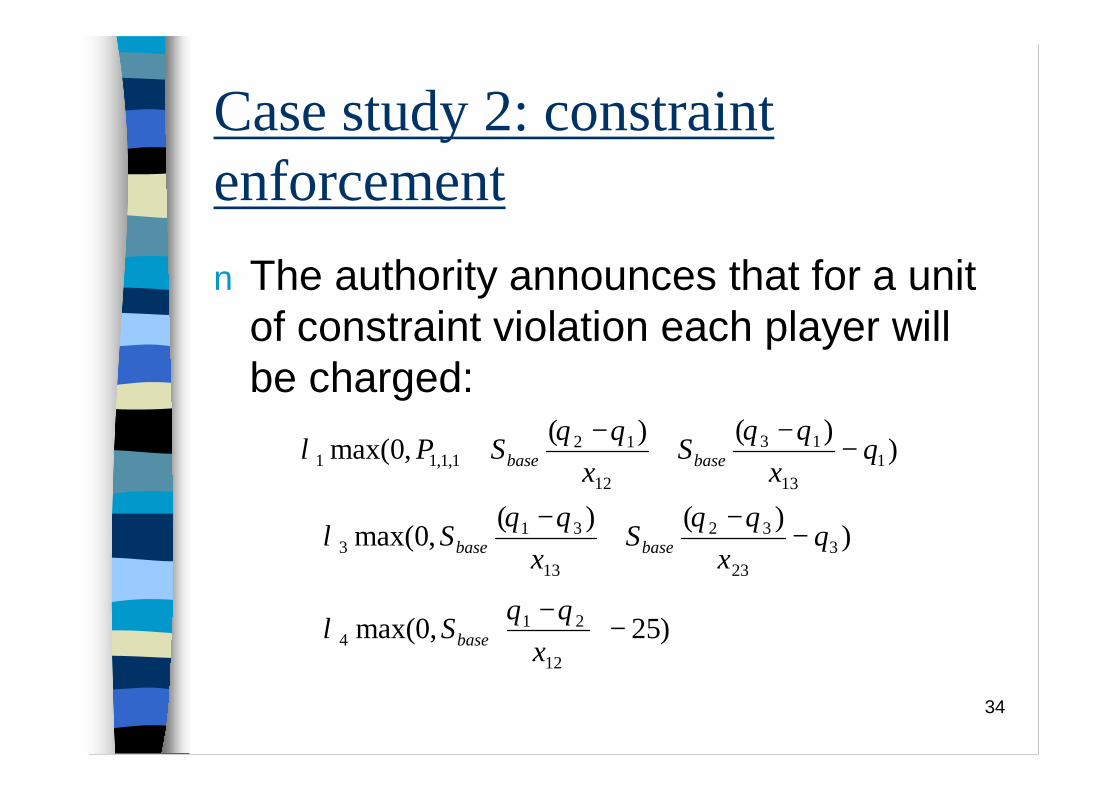
Case study 2: constraint enforcementn The authority announces that for a unit

of constraint violation each player will be charged:

)25,0max(

))()(,0max(

))()(,0max(

12

214

323

32

13

313

113

13

12

121,1,11

−

−+

−−

+−

+

−−

+−

+

xS

qx

Sx

S

qx

Sx

SP

base

basebase

basebase

θθλ

θθθθλ

θθθθλ

35

Case study 2: constraint enforcementn The previous extra term is added to the

original individual payoff functions of firms 1 and 2 (slide 23)

n The same result as in case 2 is obtained, without coupling constraints (decoupled Nash equilibrium)

36

Conclusions

n A Nikaido-Isoda Relaxation Algorithm to find unique Nash-Cournot equilibria with coupled constraints

n Either a centralized or a distributed optimization viewpoint

n Applications to electricity tradingn Enforcement of constraints decouples

the problem and finds the same solution

End of the presentation

Thank you!

e-mail: Javier.Contreras@uclm.es