Embed Size (px)
Citation preview
A numerical investigation of tip clearance flowin Kaplan water turbines
M.Sc. H. Nilsson Prof. L. DavidsonChalmers University of Technology Chalmers University of TechnologyThermo and Fluid Dynamics Thermo and Fluid DynamicsS - 412 96 Gothenburg S - 412 96 GothenburgSweden [email protected] [email protected]
Introduction
A parallel multiblock finite volume CFD (Computational Fluid Dynamics) code, CALC-PMB (Parallel Multi-Block), for computations of turbulent flow in complex domains has been developed for an investigation of the tur-bulent flow in Kaplan water turbines. The main features of the code are the use of general curvilinear coordinates,pressure correction scheme (SIMPLEC [6]), cartesian velocity components as principal unknowns, and collocatedgrid arrangement together with Rhie and Chow interpolation. The computational blocks are solved in parallelwith Dirichlet-Dirichlet coupling using PVM (Parallel Virtual Machine) or MPI (Message Passing Interface). Theparallel efficiency is excellent, with super scalar speedup for load balanced applications [3]. The commercial gridgenerator ICEM CFD/CAE is used for grid generation and the commercial post-processors Tecplot and Ensightare used for post-processing.
This work is focused on tip clearance losses, which reduce the efficiency of a Kaplan water turbine by about0.5%. The investigated turbine is a test rig with a runner diameter of0:5m. It has four runner blades and 24 guidevanes. The tip clearance between the runner blades and the shroud is0:25mm. To resolve the turbulent flow inthe tip clearance and in the boundary layers, a low Reynolds numberk � ! turbulence model is used. Becauseof computational restrictions, complete turbine simulations usually use wall functions instead of resolving theboundary layers, which makes tip clearance investigations impossible.
The computational domain starts at the trailing edge of the guide vanes and ends at the inlet of the draft tube ina 90-degree section, including one runner blade, of the investigated Kaplan water turbine. This restricts the flow tobeing periodic but reduces the computational domain to 1/4 of the original size and allows stationary calculations.Complete turbine simulations commonly apply a circumferential averaging between the distributor and the runner,yielding the same periodic restriction. In reality, the inlet flow is slightly non-periodic and consists of wakes fromthe guide vanes, which results in varying angles of incidence and requires transient calculations. The present workinvestigates the flow structures of stationary periodic turbulent mean flow comparing different inlet guide vaneangles. The runner blade angles are kept at a constant value (� = 0) so that the same grid may be used for allcases. The calculations are performed in a rotating coordinate system where Coriolis and centripetal force termshave been added to the momentum equations.
The computational results from four different operating conditions with different guide vane angles are com-pared in this work. It is found that
� The computations capture a vortical structure close to the leading edge tip clearance, where the tipclearance flow interacts with the shroud boundary layer and cavitational bubbles are formed.
� The tip blade loading increases when the specific speed decreases. This is in accordance with theturbine manufacturer [9].
� The magnitude of the axial flow in the tip clearance, close to the leading edge, increases when thespecific speed decreases. This is in accordance with the tip cavitation pattern of the investigatedturbine.
� Detailed measurements need to be performed for use as boundary conditions and validation of theresults.
� Transient features of the flow should be studied using LES (Large Eddy Simulation).
The tip clearance flow pattern is in accordance with observations of the investigated turbine. However, futurework will focus on further comparisons of the computational results with measurements. Measurements will alsobe used to improve the boundary conditions. Transient calculations using LES (Large Eddy Simulation) will beperformed in order to capture the effects of the guide vane wakes and the instabilities of the tip vortex.
Case N11 Q11 ��NDpH
� �Q
D2pH
�(guide vane angle) (efficiency)
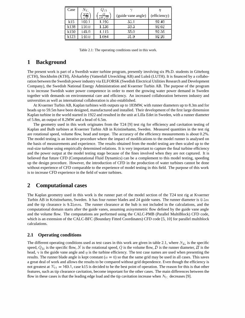
k15 160:1 1:195 35:1 92:40k138 150:0 1:136 33:3 92:62k150 145:0 1:115 33:0 92:56k123 140:0 1:084 31:9 92:26
Table 2.1: The operating conditions used in this work.
1 Background
The present work is part of a Swedish water turbine program, presently involving six Ph.D. students in G¨oteborg(CTH), Stockholm (KTH),Alvkarleby (Vattenfall Utveckling AB) and Lule˚a (LUTH). It is financed by a collabo-ration between the Swedish power industry via ELFORSK (Swedish Electrical Utilities Research and DevelopmentCompany), the Swedish National Energy Administration and Kvaerner Turbin AB. The purpose of the programis to increase Swedish water power competence in order to meet the growing water power demand in Swedentogether with demands on environmental care and efficiency. An increased collaboration between industry anduniversities as well as international collaboration is also established.
At Kvaerner Turbin AB, Kaplan turbines with outputs up to 183MW, with runner diameters up to 8.3m and forheads up to 59.5m have been designed, manufactured and installed. Their development of the first large dimensionKaplan turbine in the world started in 1922 and resulted in the unit at Lilla Edet in Sweden, with a runner diameterof 5.8m, an output of 8.2MW and a head of 6.5m.
The geometry used in this work originates from the T24 [9] test rig for efficiency and cavitation testing ofKaplan and Bulb turbines at Kvaerner Turbin AB in Kristinehamn, Sweden. Measured quantities in the test rigare rotational speed, volume flow, head and torque. The accuracy of the efficiency measurements is about 0.2%.The model testing is an iterative procedure where the impact of modifications to the model runner is analysed onthe basis of measurements and experience. The results obtained from the model testing are then scaled up to thereal-size turbine using empirically determined relations. It is very important to capture the final turbine efficiencyand the power output at the model testing stage because of the fines involved when they are not captured. It isbelieved that future CFD (Computational Fluid Dynamics) can be a complement to this model testing, speedingup the design procedure. However, the introduction of CFD in the production of water turbines cannot be donewithout experience of CFD comparable to the experience of model testing in this field. The purpose of this workis to increase CFD experience in the field of water turbines.
2 Computational cases
The Kaplan geometry used in this work is the runner part of the model section of the T24 test rig at KvaernerTurbin AB in Kristinehamn, Sweden. It has four runner blades and 24 guide vanes. The runner diameter is0:5mand the tip clearance is0:25mm. The runner clearance at the hub is not included in the calculations, and thecomputational domain starts after the guide vanes, assuming axisymmetric flow defined by the guide vane angleand the volume flow. The computations are performed using the CALC-PMB (Parallel MultiBlock) CFD code,which is an extension of the CALC-BFC (Boundary Fitted Coordinates) CFD code [5, 10] for parallel multiblockcalculations.
2.1 Operating conditions
The different operating conditions used as test cases in this work are given in table 2.1, whereN11 is the specificspeed,Q11 is the specific flow,N is the rotational speed,Q is the volume flow,D is the runner diameter,H is thehead, is the guide vane angle and� is the turbine efficiency. The test case names are used when presenting theresults. The runner blade angle is kept constant (� = 0) so that the same grid may be used in all cases. This savesa great deal of work and allows the results to be compared without grid dependence. Even though the efficiency isnot greatest atN11 = 160:1, case k15 is decided to be the best point of operation. The reason for this is that otherfeatures, such as tip clearance cavitation, become important for the other cases. The main differences between theflow in these cases is that the leading edge load and the tip cavitation increase whenN11 decreases [9].
2.2 Equations
The equations used for the computations are briefly described below.The Reynolds time-averaged continuity and Navier Stokes equations for incompressible flow in a rotating
frame of reference reads [8, 4]
@�Ui@xi
= 0
@�Ui@t
+@�UiUj@xj
=
�
@P
@xi+
@
@xj
��
�@Ui@xj
+@Uj@xi
�� �u0iu
0j
�+ �gi � ��ijk�klmjlxm � 2��ijkjUk
where��ijk�klmjlxm is the centripetal term and�2�ijkjUk is the Coriolis term, owing to the rotating co-ordinate system. Because of the potential nature of the pressure, gravitational and centripetal terms, they are puttogether in what is often referred to as areducedpressure gradient
�
@P �
@xi= �
@P
@xi+ �gi � ��ijk�klmjlxm
Thus, a relation for thereducedpressure is
P � = P � �gixi + ��ijk�klmjlxmxi
The star and the term ’reduced’ of P � are omitted in the rest of this work, and it is simply referred to as staticpressure.
The Boussinesq assumption for the Reynolds stress tensoru0iu0j reads
�u0iu0j = ��t
�@Ui@xj
+@Uj@xi
�+
2
3�ij�k
wherek = 1
2u0iu
0i is the turbulent kinetic energy. Thek� ! model of Wilcox [11] for the turbulent kinetic energy,
k, and the specific dissipation rate,!, reads
@�Ujk
@xj=
@
@xj
���+
�t�k
�@k
@xj
�+ Pk � ��?!k
@�Uj!
@xj=
@
@xj
���+
�t�!
�@!
@xj
�+!
k(c!1Pk � c!2�k!)
where the turbulent viscosity�t is defined as
�t = �k
!
The production term reads
Pk = �t
�@Ui@xj
+@Uj@xi
�@Ui@xj
�
2
3�k
@Ui@xi
and the closure coefficients are defined from experiment as
�? = 0:09, c!1 = 5
9, c!2 = 3
40, �k = 2 and�! = 2
2.3 Numerical considerations
The geometry is a four-blade and 24-guide vane Kaplan turbine. If the spiral casing distributes the flow axisym-metrically (a good assumption according to the turbine manufacturer), it is reasonable to believe that the runnerflow is periodic over an angle of 90 degrees. This assumption, together with periodic boundary conditions, reducethe computational domain to1=4th of its original size. The computational domain starts after the guide vanes, as-suming axisymmetric flow defined by the guide vane angle and the volume flow. A fully developed turbulent1=7thvelocity and turbulent kinetic energy inlet profile are assumed. The inlet turbulent lengthscale is prescribed so that
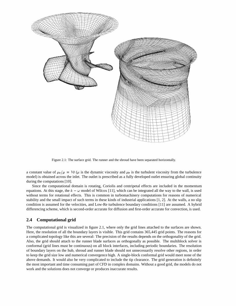
Figure 2.1: The surface grid. The runner and the shroud have been separated horizontally.
a constant value of�t=� = 10 (� is the dynamic viscosity and�t is the turbulent viscosity from the turbulencemodel) is obtained across the inlet. The outlet is prescribed as a fully developed outlet ensuring global continuityduring the computations [10].
Since the computational domain is rotating, Coriolis and centripetal effects are included in the momentumequations. At this stage, thek � ! model of Wilcox [11], which can be integrated all the way to the wall, is usedwithout terms for rotational effects. This is common in turbomachinery computations for reasons of numericalstability and the small impact of such terms in these kinds of industrial applications [1, 2]. At the walls, a no slipcondition is assumed for the velocities, and Low-Re turbulence boundary conditions [11] are assumed. A hybriddifferencing scheme, which is second-order accurate for diffusion and first-order accurate for convection, is used.
2.4 Computational grid
The computational grid is visualized in figure 2.1, where only the grid lines attached to the surfaces are shown.Here, the resolution of all the boundary layers is visible. This grid contains 365,445 grid points. The reasons fora complicated topology like this are several: The precision of the results depends on the orthogonality of the grid.Also, the grid should attach to the runner blade surfaces as orthogonally as possible. The multiblock solver isconformal (grid lines must be continuous) on all block interfaces, including periodic boundaries. The resolutionof boundary layers on the hub, shroud and runner blade should not unnecessarily resolve other regions, in orderto keep the grid size low and numerical convergence high. A single-block conformal grid would meet none of theabove demands. It would also be very complicated to include the tip clearance. The grid generation is definitelythe most important and time consuming part of CFD in complex domains. Without a good grid, the models do notwork and the solutions does not converge or produces inaccurate results.
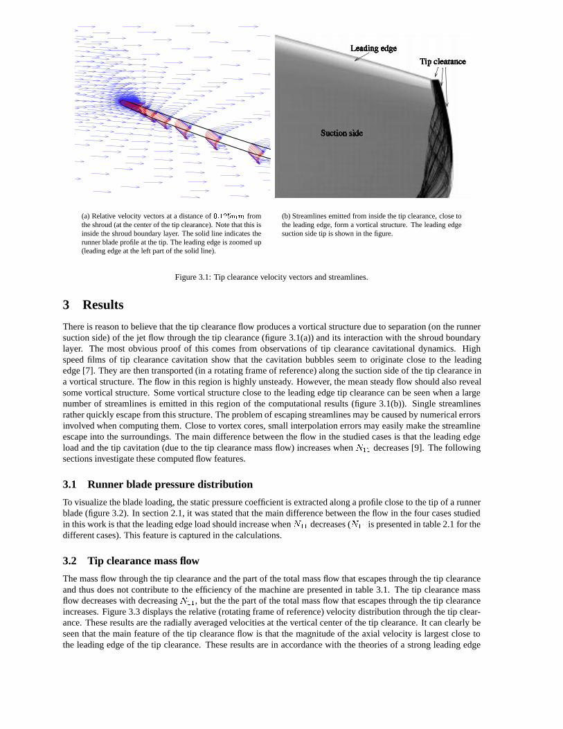
(a) Relative velocity vectors at a distance of0:125mm fromthe shroud (at the center of the tip clearance). Note that this isinside the shroud boundary layer. The solid line indicates therunner blade profile at the tip. The leading edge is zoomed up(leading edge at the left part of the solid line).
(b) Streamlines emitted from inside the tip clearance, close tothe leading edge, form a vortical structure. The leading edgesuction side tip is shown in the figure.
Figure 3.1: Tip clearance velocity vectors and streamlines.
3 Results
There is reason to believe that the tip clearance flow produces a vortical structure due to separation (on the runnersuction side) of the jet flow through the tip clearance (figure 3.1(a)) and its interaction with the shroud boundarylayer. The most obvious proof of this comes from observations of tip clearance cavitational dynamics. Highspeed films of tip clearance cavitation show that the cavitation bubbles seem to originate close to the leadingedge [7]. They are then transported (in a rotating frame of reference) along the suction side of the tip clearance ina vortical structure. The flow in this region is highly unsteady. However, the mean steady flow should also revealsome vortical structure. Some vortical structure close to the leading edge tip clearance can be seen when a largenumber of streamlines is emitted in this region of the computational results (figure 3.1(b)). Single streamlinesrather quickly escape from this structure. The problem of escaping streamlines may be caused by numerical errorsinvolved when computing them. Close to vortex cores, small interpolation errors may easily make the streamlineescape into the surroundings. The main difference between the flow in the studied cases is that the leading edgeload and the tip cavitation (due to the tip clearance mass flow) increases whenN11 decreases [9]. The followingsections investigate these computed flow features.
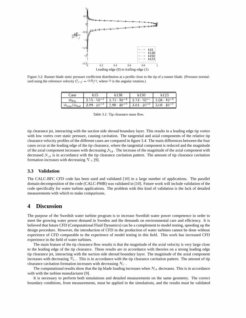
3.1 Runner blade pressure distribution
To visualize the blade loading, the static pressure coefficient is extracted along a profile close to the tip of a runnerblade (figure 3.2). In section 2.1, it was stated that the main difference between the flow in the four cases studiedin this work is that the leading edge load should increase whenN11 decreases (N11 is presented in table 2.1 for thedifferent cases). This feature is captured in the calculations.
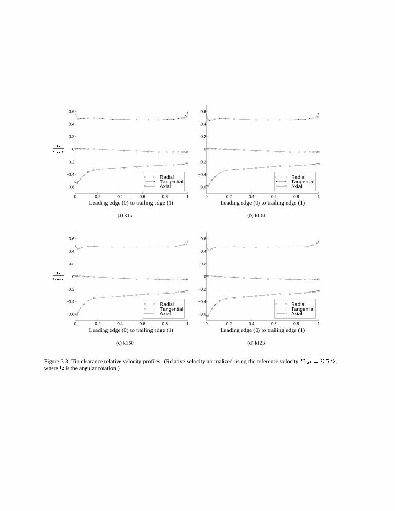
3.2 Tip clearance mass flow
The mass flow through the tip clearance and the part of the total mass flow that escapes through the tip clearanceand thus does not contribute to the efficiency of the machine are presented in table 3.1. The tip clearance massflow decreases with decreasingN11, but the the part of the total mass flow that escapes through the tip clearanceincreases. Figure 3.3 displays the relative (rotating frame of reference) velocity distribution through the tip clear-ance. These results are the radially averaged velocities at the vertical center of the tip clearance. It can clearly beseen that the main feature of the tip clearance flow is that the magnitude of the axial velocity is largest close tothe leading edge of the tip clearance. These results are in accordance with the theories of a strong leading edge
0 0.2 0.4 0.6 0.8 1−2.5
−2
−1.5
−1
−0.5
0
0.5
1
k15 k138k150k123
2P�C2
ref
Leading edge (0) to trailing edge (1)
Figure 3.2: Runner blade static pressure coefficient distribution at a profile close to the tip of a runner blade. (Pressure normal-ized using the reference velocityCref = D=2, where is the angular rotation.)
Case k15 k138 k150 k123_mtip 2:15 � 10�4 2:12 � 10�4 2:12 � 10�4 2:08 � 10�4
_mtip= _mtot 2:88 � 10�3 2:98 � 10�3 3:04 � 10�3 3:08 � 10�3
Table 3.1: Tip clearance mass flow.
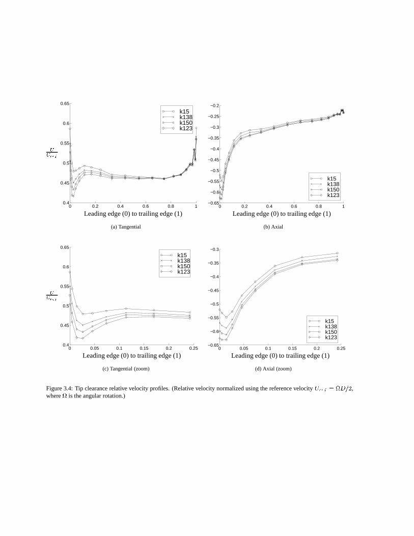
tip clearance jet, interacting with the suction side shroud boundary layer. This results in a leading edge tip vortexwith low vortex core static pressure, causing cavitation. The tangential and axial components of the relative tipclearance velocity profiles of the different cases are compared in figure 3.4. The main differences between the fourcases occur at the leading edge of the tip clearance, where the tangential component is reduced and the magnitudeof the axial component increases with decreasingN11. The increase of the magnitude of the axial component withdecreasedN11 is in accordance with the tip clearance cavitation pattern. The amount of tip clearance cavitationformation increases with decreasingN11 [9].
3.3 Validation
The CALC-BFC CFD code has been used and validated [10] in a large number of applications. The paralleldomain decomposition of the code (CALC-PMB) was validated in [10]. Future work will include validation of thecode specifically for water turbine applications. The problem with this kind of validation is the lack of detailedmeasurements with which to make comparisons.
4 Discussion
The purpose of the Swedish water turbine program is to increase Swedish water power competence in order tomeet the growing water power demand in Sweden and the demands on environmental care and efficiency. It isbelieved that future CFD (Computational Fluid Dynamics) can be a complement to model testing, speeding up thedesign procedure. However, the introduction of CFD in the production of water turbines cannot be done withoutexperience of CFD comparable to the experience of model testing in this field. This work has increased CFDexperience in the field of water turbines.
The main feature of the tip clearance flow results is that the magnitude of the axial velocity is very large closeto the leading edge of the tip clearance. These results are in accordance with theories on a strong leading edgetip clearance jet, interacting with the suction side shroud boundary layer. The magnitude of the axial componentincreases with decreasingN11. This is in accordance with the tip clearance cavitation pattern. The amount of tipclearance cavitation formation increases with decreasingN11.
The computational results show that the tip blade loading increases whenN11 decreases. This is in accordancewith with the turbine manufacturer [9].
It is necessary to perform both simulations and detailed measurements on the same geometry. The correctboundary conditions, from measurements, must be applied in the simulations, and the results must be validated
0 0.2 0.4 0.6 0.8 1
−0.6
−0.4
−0.2
0
0.2
0.4
0.6
Radial TangentialAxial
UUref
Leading edge (0) to trailing edge (1)
(a) k15
0 0.2 0.4 0.6 0.8 1
−0.6
−0.4
−0.2
0
0.2
0.4
0.6
Radial TangentialAxial
Leading edge (0) to trailing edge (1)
(b) k138
0 0.2 0.4 0.6 0.8 1
−0.6
−0.4
−0.2
0
0.2
0.4
0.6
Radial TangentialAxial
UUref
Leading edge (0) to trailing edge (1)
(c) k150
0 0.2 0.4 0.6 0.8 1
−0.6
−0.4
−0.2
0
0.2
0.4
0.6
Radial TangentialAxial
Leading edge (0) to trailing edge (1)
(d) k123
Figure 3.3: Tip clearance relative velocity profiles. (Relative velocity normalized using the reference velocityUref = D=2,where is the angular rotation.)
0 0.2 0.4 0.6 0.8 10.4
0.45
0.5
0.55
0.6
0.65
k15 k138k150k123
UUref
Leading edge (0) to trailing edge (1)
(a) Tangential
0 0.2 0.4 0.6 0.8 1−0.65
−0.6
−0.55
−0.5
−0.45
−0.4
−0.35
−0.3
−0.25
−0.2
k15 k138k150k123
Leading edge (0) to trailing edge (1)
(b) Axial
0 0.05 0.1 0.15 0.2 0.250.4
0.45
0.5
0.55
0.6
0.65
k15 k138k150k123
UUref
Leading edge (0) to trailing edge (1)
(c) Tangential (zoom)
0 0.05 0.1 0.15 0.2 0.25−0.65
−0.6
−0.55
−0.5
−0.45
−0.4
−0.35
−0.3
k15 k138k150k123
Leading edge (0) to trailing edge (1)
(d) Axial (zoom)
Figure 3.4: Tip clearance relative velocity profiles. (Relative velocity normalized using the reference velocityUref = D=2,where is the angular rotation.)
against measurements. This will be included in future work.The grid generation is definitely the most important and time consuming part of CFD in complex domains.
Without a good grid, the models do not work and the solutions do not converge or gives inaccurate results. Inorder to reduce grid generation time and optimize grid quality, automatic grid generation templates for each waterturbine type should be generated. This is especially important when comparing different runner blade angles.
The flow in water turbines is highly transient due to the guide vane wakes and the inherent instabilities down-stream. Some of the features of the flow cannot be captured using Reynolds averaged methods. With LES (LargeEddy Simulation), these features may be investigated. This will be included in future work.
References[1] S. Baralon. Private communication.Dept. of Thermo and Fluid Dynamics, Chalmers University of Technology, 1998.
[2] J. Bredberg. Private communication.Dept. of Thermo and Fluid Dynamics, Chalmers University of Technology, 1999.
[3] S. Dahlstrom, H. Nilsson, and L. Davidson. Lesfoil: 6-months progress report by Chalmers. Technical report, Dept. ofThermo and Fluid Dynamics, Chalmers University of Technology, Gothenburg, 1998.
[4] L. Davidson. An introduction to turbulence models. Int.rep. 97/2, Thermo and Fluid Dynamics, Chalmers University ofTechnology, Gothenburg, 1997.
[5] L. Davidson and B. Farhanieh. CALC-BFC: A finite-volume code employing collocated variable arrangement and carte-sian velocity components for computation of fluid flow and heat transfer in complex three-dimensional geometries. Rept.92/4, Thermo and Fluid Dynamics, Chalmers University of Technology, Gothenburg, 1992.
[6] J.P. Van Doormaal and G.D. Raithby. Enhancements of the SIMPLE method for predicting incompressible fluid flows.Num. Heat Transfer, 7:147–163, 1984.
[7] M. Grekula. Private communication.Dept. of Naval Architecture and Ocean Engineering, Division of Hydromechanics,Chalmers University of Technology, 1999.
[8] P.K. Kundu.Fluid Mechanics. Academic Press, San Diego, California, 1990.
[9] B. Naucler. Private communication.Kvaerner Turbin AB, 1998.
[10] H. Nilsson and L. Davidson. CALC-PVM: A parallel SIMPLEC multiblock solver for turbulent flow in complex domains.Int.rep. 98/12, Dept. of Thermo and Fluid Dynamics, Chalmers University of Technology, Gothenburg, 1998.
[11] D.C. Wilcox. Reassessment of the scale-determining equation for advanced turbulence models.AIAA J., 26(11):1299–1310, 1988.
Biographical details of the authors
H. Nilsson graduated in Physical Oceanography from the University of Gothenburg in 1997. Since that time, hehas been a Ph.D student at Chalmers University of Technology, Gothenburg, where he specializes in numericalsimulation of turbulent flow in Kaplan water turbines using parallel super computers.
L. Davidson is Professor of Heat Transfer at Chalmers University of Technology, Gothenburg, where he specializesin numerical turbulence modelling. He is supervisor for H. Nilsson.