Computers & Fluids Vol. 16, No. 1, pp. 47-58, 1988 0045-7930/88 $3.00+0.00 Printed in Great Britain. All fights reserved Copyright © 1988 Pergamon Journals Ltd

A N U M E R I C A L G R I D G E N E R A T I O N T E C H N I Q U E

B. H. GILDING'~

Faculty of Applied Mathematics, University of Twente, Enschede, The Netherlands

(Received 25 February 1987)

AIBIrjet--The paper describes a technique for the generation of boundary-fitted ¢urvilinear coordinate systems for the numerical solution of partial differential equations in two space dimensions. The technique is algebraic, has a transfinite character, and is based on the blending of shearing transformations. Applications to numerical grid generation for problems in the field of computational fluid dynamics are presented.

1. I N T R O D U C T I O N

The considerable progress in the numerical solution of partial differential equations on regions with arbitrarily-shaped boundaries in recent years has been greatly abetted by the development of techniques for numerical grid generation. This is especially true in the field of computational fluid dynamics, but also applies to other areas, such as heat transfer, mass transport, electromagnetism, solid mechanics, and structures [1-4].

Basically, techniques for numerical grid generation can be divided into two classes, viz. techniques which themselves involve solving partial differential equations, and algebraic interpolation techniques. In general, the preference for a technique involving the numerical solution of a partial differential equation above an algebraic technique is that it generates a smoother grid in which the propagation of boundary slope discontinuities is alleviated~ On the other hand, algebraic techniques provide explicit grid control and, in comparison to the other class of techniques, require relatively few computations. Subsequently, in implementation, they have the advantage of speed and simplicity. This also makes them particularly attractive for use in conjunction with interactive computer graphics and for the generation of grids for simulations involving time-varying problem domains [2-6].

In this paper, a new algebraic technique for the generation of boundary-fitted curvilinear coordinate systems for numerically solving partial differential equations in two space dimensions is presented. The technique may be classified as transfinite in the sense that it involves interpolation between the trajectories of the boundary curves defining a problem domain. In other words, as opposed to a finite number of points, the coordinate system is generated by a non-denumerable number of boundary points. Notwithstanding, the technique does not conform to the standard concept of transfinite interpolation--it cannot be formulated in terms of the Boolean sum of a sequence of univariate projections [2-5, 7]. The technique has some affinity with the linear two-boundary technique with side constraints described in Ref. [5] and referred to in Ref. [3]. However, the technique may best be regarded as a kind of blended shearing transformation. Indeed, it arose out of the desire to extend a shearing transformation in which the coordinates of the computational points in a grid were obtained simply by normalizing a given boundary distribution between two other adjoining boundaries, to situations in which a blended normalization would take place from the first boundary to a fourth boundary completing the demarcation of the problem domain.

The technique described in this paper was actually developed in response to a desire to generate a computational grid such as that shown in Fig. 1. This mesh stems from an application of a computer program for the solution of the Navier-Stokes equations in two space dimensions using a finite difference technique based on curvilinear coordinates. Details of the computer program together with further applications can be found in Ref.

~'Former affiliation: Delft Hydraulics Laboratory, Delft, The Netherlands. C.A.F, 16/I--D

47

48 B.H. GILDING

~ 6

) -

o

24

21

18

15

W 9

6

3

0

(o)

( b )

I I 0 3

I I I I I I I I I 6 12 18 24 30 36 42 48 54

X ( M )

I I I I I I I I I I I I I I 9 12 15 18 21 24 27 50 33 36 59 42 45 48 51 5,0,

XI

(c)

6

>-

o i o

I I I I I I I I I 6 12 18 24 30 36 42 48 54

X ( M )

Fig. I. Grid for computation of flow under a barge in a lock (a) physical boundary (b) computational domain (c) mesh.

[8]. This particular application was the computation of the flow under a barge moored in a lock, during the filling of the lock, with a view to calculating the forces exerted on the mooring ropes. The mesh represents a portion of a vertical profile lengthwise through the lock with inflow on the left and with the indentation in the upper boundary corresponding to the bow of the barge. The intersections of the lines in Fig. l(c) indicate the location of computational points for the finite difference solution of the Navier-Stokes equations. This nodal distribution was motivated by a consideration of the expected flow pattern and the corresponding desired numerical accuracy, and of simplicity.

The salient feature of the numerical grid generation technique illustrated in Fig. 1 is the blending of the normalization between the upper and lower boundaries of the distributions of points on the left- and right-hand boundaries of the problem domain. A similar blending of the point distributions on the upper and lower boundaries also occurs. However, due to the choice of an identical horizontal spacing in this example this blending is not manifest.

The foundations of the technique will be described in the next section. This will be cast in the form of a transformation of an arbitrarily-shaped simply-connected problem domain into a rectangular computational domain. In the subsequent section, the extension of the theory to problem domains containing "obstacles" and "islands" and in which the corresponding computational domain consists of a union of a number of rectangles will be presented. The extension enables a grid to be generated in an arbitrary block-structured multiply-connected physical domain without requiring the specification of a domain decomposition by the user.

A numerical grid generation technique 49

10

0

- I 0

- 3 0

- 4 0

- 5 0

t.- W

(a)

(b)

20 I 15

10

5

0

I I 10 20

I I 1 30 40 50 60

X ( M )

I 70

I I 80 90

'10

I I I I I I i I I I I I I I I I I I I 0 5 10 15 20 25 30 35 40 45 50 55 60 65 70 75 80 85 90

xr (c)

- I0

-20 >-

-30

-40

-50 I I I I I I I I I I O 10 20 30 4 0 50 60 70 80 9 0

X(M)

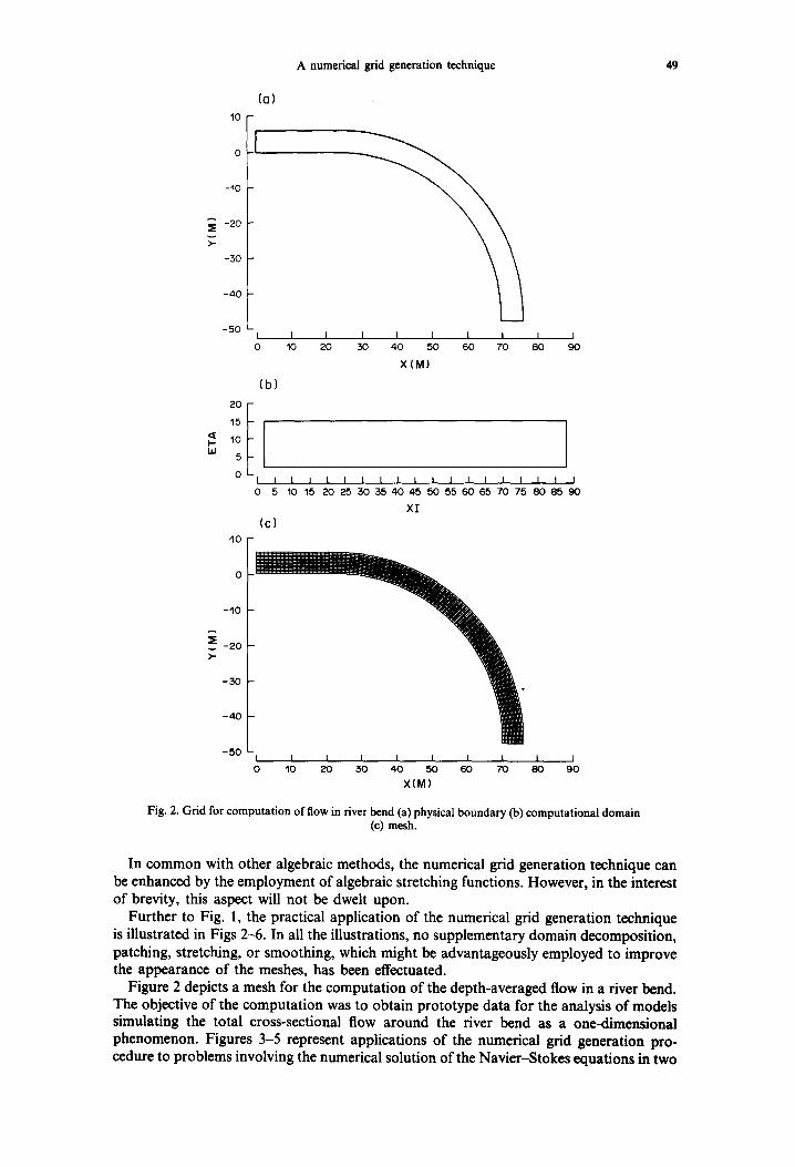
Fig. 2. Grid for computation of flow in river bend (a) physical boundary (b) computational domain (c) mesh.

In common with other algebraic methods, the numerical grid generation technique can be enhanced by the employment of algebraic stretching functions. However, in the interest of brevity, this aspect will not be dwelt upon.

Further to Fig. 1, the practical application of the numerical grid generation technique is illustrated in Figs 2-6. In all the illustrations, no supplementary domain decomposition, patching, stretching, or smoothing, which might be advantageously employed to improve the appearance of the meshes, has been effectuated.

Figure 2 depicts a mesh for the computation of the depth-averaged flow in a river bend. The objective of the computation was to obtain prototype data for the analysis of models simulating the total cross-sectional flow around the river bend as a one-dimensional phenomenon. Figures 3-5 represent applications of the numerical grid generation pro- cedure to problems involving the numerical solution of the Navier-Stokes equations in two

50 B.H. GILDING

i > -

(a) :IE: O L

1 160

b ~ c

f

g f I I I I I I I I

320 480 640 800 960 1120 'f 280 1440

X ( M )

I-- LU

24

21

18

15

12

9

6

5

0

(b)

a b

I

h g d Ic

,I le I I I I I I I I I I I I I I I I 1 I

0 5 6 9 12 15 18 21 24 27 30 33 56 39 42 45 48 ,51 54

X I

(c)

160 v ).-

o q - / I I I t I 1 I I t 160 320 480 640 800 960 1120 1280 1440

X ( M )

Fig. 3. G r i d for c o m p u t a t i o n o f f low in j u n c t i o n o f t w o w a t e r w a y s (a) physica l b o u n d a r y (b) c o m p u t a t i o n a l d o m a i n (c) mesh.

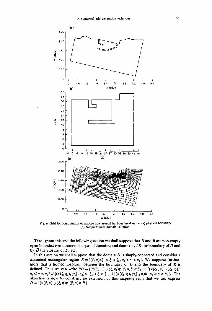
space dimensions discussed in Ref. [8]. The configuration shown in Fig. 3, for instance, stems from the simulation of the change in flow pattern in a canal which would result from the construction of a hydropower station with an outlet on the canal. The tapered arm of the mesh corresponds to the projected outlet of the hydropower station, whilst the other arms represent the existing course of the canal. Figure 4 derives from a model of the coastal flow around the Amsterdam harbour entrance near Ijmuiden in North Holland. The interest here was in the erosion and sedimentation in the area. With the grid representing a total area of 13 x 7 km, the area protected by the harbour breakwaters was simulated as a single coastal obstacle. The last figure in this group, Fig. 5, results from a study into the scour around a pipeline on the sea bottom. In this case, the objective was to reproduce a laboratory experiment in which there was a current from left to right in the picture, and as a result of scouring of bottom material, the pipeline became suspended above the sea bed. The final illustration, Fig. 6, constitutes the most involved network of the examples presented. This network was generated for modelling the inshore flow pattern to be expected from the construction of breakwaters at Sabratah in Libya. The breakwaters had been designed to protect the harbour against heavy seas; and the goal of the modelling was to ascertain their effectiveness in also mitigating the fouling hazard to shipping caused by pestilent sea-weed growth in the area. A novel feature of this mesh is that it was so designed that it could easily function for the simulation of the present situation without the harbour breakwaters by completion of the blank portions. This facilitated easy comparison of the flow pattern in the present and projected situations, cf. Ref. [9].

A numerical grid generation technique 51

A further application of the numerical grid generation technique involving patching, for the computation of tide- and wave-induced currents in a coastal zone, is to be found in Ref. [9].

Practical experience has borne out that the numerical grid generation technique described in this paper compares favourably with techniques involving the numerical solution of a partial differential equation. Compared with these more sophisticated techniques, two principal advantages have been identified. Firstly, the technique is computationally more economical. Secondly, the structure of the generated mesh is more easily controlled, particularly by the specification of computational points on the boundary or in the interior of the problem domain [9]. The technique provides an alternative to other algebraic grid generation techniques.

( a )

6.40

A 4.80

)"- 3.20

1.60

50

2 8 -

2 6 -

2 4 -

2 2 -

2 0 -

1 8 -

1 6 - LU

1 4 -

12 ~

1 0 - i 8 -

i 6 -

I 4 -

2 L

I I I I I 0 1.6 3.2 9.6 11.2 12.8 14.4

(b)

1 I I 4.8 6,4 8,0

X (KM)

1 1 I I I I I I I I I I I I I 2 4 6 8 10 12 ~4 16 18 20 22 24 26 28 30 32 34

(c ) x1

6.4o I / I I 111 [17YUHq-T~ lq - l ] I

o 80 -i'"'" ; I / l l [ l l . i i

I I I I I I I I I I 0 1 . 6 3 . 2 4 . 8 6 . 4 8 0 9 , 6 1 1 , 2 1 2 . 8 1 4 . 4

X ( K M )

Fig . 4. Grid for computation of coastal flow around harbour area protected by breakwaters (a ) physical boundary (b) computational domain (c) mesh.

52 B.H. GILDING

016 - (a)

0.12 -

:~ O . O e - v >,.

0 0 4 -

0 --

hi

I I I I I I I I I I -0.12 - 0 0 8 - 0 0 4 0 0 0 004 0.08 0.12 0.16 0.20 0.24

X ( M )

24

22

20

18

16

14

12

10

8

6

4

2

(b)

I I I I I I I I I I I I I I I 2 4 6 8 10 12 14 16 18 2(3 22 24 26 28 30 32 34 36 38

Xl

(C)

0.16 [-

o 1 2 - I ~ ~ - [ [llll[llllll[ll 111 ~ I

i o . o 8 ! - =- 0.04~ ___--

O ~

I I I I I I I I -012 -0.08 - 0 0 4 0.00 0.04 0 0 8 0.12 0.16 0.20 024

X ( M )

Fig. 5. G r i d for c o m p u t a t i o n o f f l o w a r o u n d p ipe o n sea bed (a) phys i ca l b o u n d a r y (b) c o m p u t a t i o n a l d o m a i n (c) m e s h .

2. T H E O R E T I C A L F O U N D A T I O N

Consider a problem domain D in a physical plane defined in terms of a Cartesian coordinate system (x, y). Suppose that we can specify a homeomorphism of the boundary of D onto the boundary of a canonical region R defined in terms of a coordinate system (~, t/). Then the objective of numerical grid generation as considered here is to construct an extension of the boundary transformation to a homeomorphism between the closure of D and the closure of R. The coordinates (~, t/) then constitute a boundary-fitted curvilinear coordinate system and define a computational plane. Simultaneously, the specification of a uniform grid on R in the computational plane generates a numerical grid in the physical problem domain.

3.00

0 I

2,40

~ '120

o.6o !

1 I 1 I I I I I 0.6 1.2 1.8 2.4 3 3.6 4.2 4.8

( b ) X (KM)

36

33

30

27

l-- bJ

(a)

24

;:'1

'18

15

'12

9

6

3

0 - I I

0 3

(c)

A numerical grid generation technique 53

, [ ' -

I I I I 1 I I I 1 I I I I I 6 9 12 15 18 21 24 27 30 33 36 39 42 45

X I

I 5.4

:3.00

2.40

1.80

1.20

0.60

0 I I ' l I I I I I I I 0 0.6 1.2 1.8 2.4 3 3.6 4.2 4.8 5.4

X (KM)

Fig. 6. Grid for computation of inshore flow around harbour breakwaters (a) physical boundary (b) computational domain (c) mesh.

Throughout this and the following section we shall suppose that D and R are non-empty open bounded two-dimensional spatial domains; and denote by OD the boundary of D and by D the closure of D, etc.

In this section we shall suppose that the domain D is simply-connected and consider a canonical rectangular region R = {(~,q):~l < ~ < ~2, ql < ~ < q2}. We suppose further- more that a homeomorphism between the boundary of D and the boundary of R is defined. Thus we can write aD = {(x(~, r/i), y(~, rh)): ~l ~< ~ < ~2} U {(x(~2, q), Y(~2, q)): r/i ~<q < q~} U {(x(~,q2),y(~, rh)): ~2~ ~ > 41} U {(X(~,, ~/),y(~,,r/)): r/2~> r/ >rh}. The objective is now to construct an extension of this mapping such that we can express /~ = {(x(~, q), y(~, r/)): (~, r/) e ~ } .

54 B.H. GILDING

For each point (~, r / )e/~ let ~(~, r/) denote the normalized projection of the point (x(~:,r/),y(~,q)) onto the line connecting the points (x (~ t , r / ) , y (~ ,q ) ) and (x(~,r /) ,y(~2,r /)) in the physical plane. The equation of the line joining the two last-mentioned points is:

where

and

,L(,~){y - y(¢, , ,1)} = ,~, (,~){x - x(~,, ,~)},

~ ( ~ ) = x (¢~ , ,1) - x ( ~ , , ,7) (1)

Set

and

and

ey(~) = y(~, rh) -- y(~, r/, ).

~(¢) = ~(¢, r/~) for i = 1, 2,

and

/~,(q) =/~(~, q) for i = 1,2.

Observe that for i = 1, 2; ~(~) is defined and continuous for ~ ~< ¢ ~ ~2 with ~ ( ~ ) = 0 and ~ ( ~ ) = 1. Similarly for i = 1,2; /~(q) is defined and continuous for ql ~< q ~< q~ with /~(~,) = 0 and/~(r/~) = 1.

The essence of the present technique is that we now blend the normalized projections by prescribing:

~(~, q) = {1 -/~(~, t/)}~, (¢) +/~(~, t/)~2(~),

fl(~, q) ---- {1 -- 0c(~, q)}fl, (q) + o~(~, q)fl2(rl),

for all (~, ~/)e R. Elimination of unknowns in these two equations yields:

~(~, r/) = [{1 - /~ , (q)}~, (¢) + if, (fl)~2(¢)]/d(~, q) ( l l )

(lO)

6y(rl ) = Y(~2, q) - Y({ , , q ). (2)

Hence, the normal to this line, projecting the point (x({, t/),y(¢, q)) onto it, is:

6,(~){y - y ( ~ , ~)} = -6x(~){x - x ( ¢ , ~)}.

This gives the point (x,, y,) of the projection on the line as:

x,(~, n) = x(~, , n) + ~(~, q) 6x(n) (3)

Y,(¢, q) = Y(~,, n) + ~(~, q) 6,(r/) (4)

when

~(~,n)=[{x(~,,1)-x(~,,n)}ax(,1)+{y(~,n)-y(~.,n)}6y(,t)]/[ax(,t)2+6y(n)2]. (5)

Similarly, one can define the normalized projection of the point (x(~, q), y(¢, r/)) onto the line with end-points (x(~, ql),y(~, rh)) and (x(~, q~),y(~, th)) as:

xa(¢, n) = x(~, q,) + fl(~, n) ¢x(~) (6)

yp(~, r/) = y(~, ql) + fl(~, q) ey(~), (7)

where

~(~,r l )=[{X(~,r l ) - -X(~,rh)}Ex(~)+{y(~,r l ) - -y(~,q , )}E,(¢)] /[Ex(~)2+Ey(~)2] , (8)

Ex(~) = x(¢, rh) - x(¢, q,) (9)

A numerical grid generation technique 55

and

where

/~(~, ~) = [{1 - ~, (~)}fl , (n) + ~, (¢)/~2(n)]/d(¢, ,~),

d(¢, q) = 1 -- {~2(~) -- ~x~(~)} {fl2(q) -- fl,(q)},

(12)

(13)

by which means ~(~, q) and fl(~, q) are defined for all (~, ~/)e g . Note that if 0<0q(~) , ~2(~)<1 and 0<fl~(q), f l2(r/)<l then the denominator

(13) in expressions (11) and (12) is non-zero. Consequently, it can also be shown that 0 < ct(~, q) < 1 and 0 < fl(~, r/) < 1. Moreover, if ~l(~) = ~2(~) for some ~ e [¢1, ~2], then expression (11) reduces to ~(¢,~/)=~q(~)=~t2(~) for all r/e[r/l,r/2 ]. Similarly, if ill(r/) =#20/) for some r/~[r/l,r/2], then (12) reduces to f l(~,q)=/~t(q)=fl2(r /) for all

With 0t (~, r/) and fl (~, r/) defined by (11)-(13), inversion of (5) and (8) subsequently yields the proposed boundary-fitted mapping from R to D:

x(~, r/) = [{x,(¢, rl)6~(n) +y , (~ , ~/)6y(n)}~r(~)

-- {xt~(~, rl)ex(~) + yo(~, tl),y(~)}fy(tl)]/A(~, tl ) (14)

Y(~, q) = [{x0(~)e~(~) + YO(~, rl)ey(~)]rx(n)

- {x,(~, n)fx(rl) + y,(~, rl)ry(rl)}ex(~)]/a(~ , rl), (15)

in which x,(~, r/), y~(~, r/), xa(~,~/) and y~(~, ~/) are defined by (3), (4), (6) and (7) respectively, and

a ( ~ , ,1) = ~x(n)Ey(~) - Ex(~)rA,1) . (16)

Meshes generated by application of this technique as described above are illustrated in Figs 1 and 2. We remark that a mesh generated with this technique is invariant under rotation and under scaling of both of the coordinate axes in the physical plane, but not necessarily under scaling of only one of the coordinate axes.

The potential weakness of the numerical grid generation technique described in this section lies in the use of the projection of the curves in the physical plane defined by ~ = ~' and ~/= q' onto the lines joining their end-points. If these projections are poorly defined, the technique may break down. For instance, if the computational domain contains a point (~', r/') such that in the physical plane the lines joining the end-points of the curves defined by ~ = ~" and r /= r/" are parallel, then the technique will not work since the denominator (16) in expressions (14) and (15) will become zero. Similarly, if the projection of a boundary curve onto the line joining its extremities is not one-to-one, the technique may fail to generate a satisfactory grid. Such difficulties can be avoided by exercising some additional control of the numerical grid. This can be achieved by, for example, specifying the physical coordinates of a number of points or curves in the interior of the problem domain and treating these as fictive boundaries which together with the original boundaries define a new domain, and then applying the extension of the technique described in the next section to the adapted domain.

3. EXTENSION TO MORE COMPLICATED SITUATIONS

Up to now, the discussion of the theoretical basis of the numerical grid generation technique has been restricted to the generation of a boundary-fitted grid on a simply- connected domain by considering a canonical rectangular region in the computational

plane. In this section, we shall present the extension of the theoretical basis to more irregular physical domains in which corresponding computational domain consists of the union of a number of rectangles.

56 B.H. GILDING

We consider a canonical region R defined in terms of a coordinate system (~, r/) satisfying the following criterion. For each (~, q ) • R let

~,(~, q) = inf{~': (¢", r t ) • R

~2(~, 7) = sup{~': (¢", ~) • R

7, (¢, t/) = inf{7': (~, 7") • R

q~(~, 7) = sup{7 ': (~, q " ) • R

for all ~"e (~', ¢]}

for all ¢ " • [¢, ~')}

for all 7 " • (q', r/]}

for all q" • [7, r/')};

then the total set of coordinate values ~(~, 7), (~, q ) • R, i = I, 2, consists of a finite partition, a0 < al < a~ < • • • < a., and the total set of coordinate values 7~(~, 7), (~, q) • R, i = 1, 2, consists of a finite partition, b0 < b~ < b2 < • • • < b,.. It follows that we can state that

R = U (a,_l,a,) x (b]_,,bj) U (a,_l,a,) x [bj, bj] (i,j) e ll (i ,j)~ l 2

U [a,, ,,,] x (6- , , b~) U [',,, ,,,] × [6, 6] (i,J) ~ 13 (i,J) ~ I 4

for some or other (sub)collections of pairs of indices (i,j) with 1 ~< i < n and 1 < j ~< m; I~, 12, 13 and 14 say. Moreover, given R, this is the smallest union of rectangles with this property. Examples of such canonical regions R are given in Figs l(b), 2(b), 3(b), 4(b), 5(b) and 6(b). The boundary of R may contain isolated points and isolated curves corresponding to slits in the physical domain. A problem domain D defined in the physical plane is characterized by the existence of a homeomorphic mapping from the boundary of R onto the boundary of D, viz. one has specified OD = {(x(~, q), Y(~, 7)):(~, 7 ) • OR }.

Note that by definition, given any point (~, 7) • R, i f j i s such that b~_ ~ ~< q < bj; although (t (~, 7) and ~2(~, 7) may span several segments of the partition a0, a~ . . . . . a.; the points (~, (~, ~/), bj_ ,), (~2(~, 7), bj_l), (~1 (~, 7), bj), and (~(~, 7), b~) e 0R; whilst the rectangle (~l (~, q), ~2(~, q)) x (b~_ ~, b~) is wholly contained in R. Hence, f o r j = 1, 2 . . . . . m, we can inductively define:

• 1 (~, 7) = [{x(~, b~_l ) - x(~, (~, 7), b~_ ,)}&x, 1

+ {y(¢, bi_l) - Y ( ¢ t ( { , q), b~-O}ay,,]/[6~,, + 62.1]

where

and

6x,1 = x(~2(~, ~), bi_1) - x(~, (~, ~), bj_ 1)

6y,, = Y(~2(~, 7), bj_ ,) - Y(~I (~, 7), bj_ ,)

x ( ~ , b j _ l ) - - - lira [X(~I(~,7),~)'~-~I(~,t~){X(~2(~,7),7)--X(~I(~,7),7)}] ,tb s -~

y(~, bs_ ,) = lim [Y(~I (~, 7), q) + al (~, 7){Y(~2(~, 7), 7) - Y(~, (~, 7), 7)}] , tb- t

if (~ ,bj_l )~OR,

for all (~, ~/) • R with bj_ 1 <<. ~l < bj. Similarly, we can inductively define

a~(¢, 7) = [{x(¢, bj) - x(~X, (¢, 7), bj)}hx.2 + {y(¢, bj) -Y(¢1(¢, 7), bj)I6y.2]/[6~,2 + ay2,2]

where

6~,2 = x(~2(~, 7), bi) - x(~l (~, 7), bj)

6y,2 = Y(~2(~, 7), bj) - y ( ~ , ( ~ , 7), bj)

A numerical grid generation technique 57

and

x(~. b~) = lim [x(~l (¢. r/). q) + ~2(~. ~/) {x(~2(~. r/). r/) - x(~. (~. r/). q)}]

y(~. b~) = lira [Y(~I (~. , ) . r/) + ~ (¢ . r/){Y(~2(~, q). ~/) - Y ( ~ I (~. r/). r/)}] ~bj

if (~, b~) ~ OR,

for all (~, r/) ~ R with bg >1 r / > b~_ 1, for j = m, m - 1, m - 2 . . . . . 1. Likewise, given any (~, r/)~ R, if i is such that ai_ 1 ~< ~ ~< ai; al though r/i (~, r/) and r/2(~, r/) may span several segments of the parti t ion b0, bl . . . . , b,,; the points (a~_ 1, rh (~, r/)), (ai_ 1, r/~(~, r/)), (as, ql(~, q)), and (ai, r/2(~, r/)) ~ OR, whilst the rectangle (a;_ 1, al) x (r/l(~, r/), r/2(~, q)) is wholly contained in R. So that, for i = 1, 2 . . . . . n, we can inductively define

where

and

fll (~, r/) = [{x(ai_ i, r/) - x (a i_ t , rh (~, r/))}e~. 1 2 + {y (ai , i. r/) -- Y (al_, . q l (~. r/))}~. 1 ]/[e ~x., + ey.l]

E,,, 1 = x ( a i _ l , r / 2 ( ~ , r / ) ) - x (a l_ l , rh (~, r / ) )

E.y.i ~- y (a i_ l , 1'/2 (~, r/)) - y (a ,_ l , rh (~, r/))

x (a i_ l , r/) = lira

Y (ai- 1, r/) = lira ~ T a i - I

[x (~, n l (¢, r/)) + #1 (~, r/){x (~, r/2 (~, r/)) - x (~, n, (~, ,1))}]

[y(~, ql(~, r/)) + fll(~, r/){y(~, r/2(~, r/)) - y (¢ , r/l(~, q))}l

if (ai_ 1, r/) ~ OR,

for all (~, r/) e R with ai_ i ~< ~ < ai; and, for i = n, n - 1, n - 2 . . . . ,1,

f12(~, r/) = [{x(a,, r/) - x(ai , r/, (~, r/))}ex.2 + {y(ai, r/) - y(ai , r/, (~, r/))}Ey. 2I/[E~. 2 -t-/~y.212

where

and

ex.2 = x(ai , r/2(~, r/)) - x(al , r/l (~, r/ ))

Ey,2 = y (a,, r/2 ( ~, r/ )) - Y (a,, r/i ( ~, r/ ))

x(al , r/) = lim [x(~, r/, (~, r/)) + fl2(¢, r/){x(~, q2(~, r/)) - x(~, r/, (~, r/))}]

y(as, r/) = lim D'(¢, r/, (~, r/)) + f12(~, r/){y(~, r/2(~, r/)) - y ( ~ , q,(¢, r/))}] ~a~

if (as, r/) ~ OR,

for all (~, r/) e R with ai i> ¢ > ai_ 1. The formulae for the boundary-f i t ted mapping of R to D are now given by (1)-(4), (6), (7), and (9)--(16), with ct~(~) replaced by ~ti(~, r/), ill(r/) replaced by fl~(~, r/), ~i replaced by ~i(~, r/), and r/s replaced by r/s(~, r/), for i = 1, 2.

In principal, the above formulae can be used to generate a numerical grid on an arbitrari ly-shaped mult iply-connected domain wi thout further ado. Nonetheless, tests have revealed that this does not always lead to the optimal form, since, in general, as it were, the coordinates generated in a point (U, r/') will be predominant ly determined by the behaviour of the physical boundary corresponding to the lines ~ = ~ l ( ~ ' , r / ' ) ,

58 B.H. GILDING

= ~:(~ ', ~/'), ~/ = ~/l (~', ~/'), and ~/ = ~h(~', ~/') at the expense o f ignoring "obs tac les" and " is lands" in the physical plane in the ne ighbourhood of the image point (x(~ ' , ~ / ' ) ,y (~ ' , ~/')). The fo rm improves through the simple measure o f taking the grid generat ion in stages.

First, physical coordinates for those points in the computa t iona l plane ((, ~/) with the p roper ty that [~l(~, r/), ~2(~, ~/)] x [~h (~, ~/), ~h(~, ~/)] is conta ined in /~ are generated. Once the physical coordinates for these points have been generated, a new computa t iona l domain consisting of the remaining points in R is au tomat ica l ly defined, and the procedure is repeated. Since the originally-specified computa t iona l domain is composed of the union o f a finite n u m b e r of rectangles, this s t rategy need only be repeated a limited number o f times to satisfactorily generate an entire grid in the original domain .

C o m p a r e d with decompos ing D into subdomains cor responding to rectangular sub- regions o f R and subsequent ly patching meshes generated independent ly on each sub- domain , the essential feature of the extension of the grid generat ion technique described above is that it is au tomat ic . Tha t is to say, it does not require the specification of any internal dividing curves on the par t o f the user (a l though natural ly one is free to define imaginary internal boundar ies if one so wishes).

Meshes generated by the extended technique as described in this section are shown in Figs 3-6. These meshes illustrate the scope of the technique. In part icular , Figs 4 and 6 depict meshes in which the physical domain contains one or more "obs tac les" , whilst Fig. 5 depicts a mesh in which the physical domain contains an " is land". All o f these meshes are derived f rom practical appl icat ions in the field o f computa t iona l fluid dynamics which are reviewed in the In t roduct ion.

Acknowledgements--The technique described in this paper was developed whilst the author was employed by the Delft Hydraulics Laboratory. The subsequent consent of the laboratory to the publication of this work is thus gratefully acknowledged.

REFERENCES

I. J. F. Thompson (Editor), Numerical Grid Generation. Elsevier, New York (1982). 2. J. F. Thompson, Z. U. A. Warsi and C. W. Mastin, Boundary-fitted coordinate systems for numerical

solution of partial differential equations--a review. J. Comput. Phys. 47, 1-108 (1982). 3. J. F. Thompson, Grid generation techniques in computational fluid dynamics. AIAA J. 22, 1505-1523 (1984). 4. L.-E. Eriksson, Practical three-dimensional mesh generation using transfinite interpolation. SIAM J. Sci.

Star. Comput. 6, 712-741 (1985). 5. R. E. Smith, Algebraic grid generation. In: Numerical Grid Generation (Edited by J. F. Thompson),

pp. 137-170. Elsevier, New York (1982). 6. S.-L. Yang and T. I.-P. Shih, An algebraic grid generation technique for time-varying two-dimensional

spatial domains. Int. J. numer. Meth. Fluids 6, 291-304 (1986). 7. W. J. Gordon and L. C. Thiel, Transfinite mappings and their application to grid generation. In: Numerical

Grid Generation (Edited by J. F. Thompson) , pp. 171-192. Elsevier, New York (1982). 8. M. J. Oflicier, C. B. Vreugdenhil and H. G. Wind, Applications in hydraulics of numerical solutions of the

Navier-Stokes equations. In: Computational Techniques for Fluid Flow (Edited by C. Taylor, J. A. Johnson and W. R. Smith), pp. 115-147. Pineridge Press, Swansea (1986).

9. M. J. Officier and A. K. Wiersma, Experience with numerical grid generation techniques and their application in flow problems at the Delft Hydraulics Laboratory. In: Numerical Grid Generation in Computational Fluid Dynamics (Edited by J. H/iuser and C. Taylor), pp. 641~52. Pineridge Press, Swansea (1986).