Nonlinearity 3 (1990) 177-195. Printed in the UK

A numerical calculation of a weakly non-local solitary wave: the qb4 breather

John P Boyd Department of Atmospheric and Oceanic Science and Laboratory for Scientific Computation, University of Michigan, 2455 Hayward Avenue, Ann Arbor, MI 48109, USA

Received 2 May 1989 Accepted by J F Toland

Abstract. The breather of the +4 field theory decays by radiation to infinity. The concept of a solitary wave is still useful, however, because a, the amplitude of the ‘far field’ radiation, is exponentially small in E , the breather amplitude. (The phrase ‘weakly non-local’ in the title means that the quasisoliton has non-zero but very tiny amplitude as 1x1- m.) In this paper, we introduce novel numerical methods to compute G4 breathers. We calculate solutions both on a finite, spatially periodic interval and on

We find that spatially periodic breathers are permanent and non-decaying. If we relax the requirement that the soliton decay exponentially for large 1x1, we may also compute non-decaying, weakly non-local breathers on the infinite interval, too. The latter computation requires a mixed spectral basis of rational Chebyshev functions and a special ‘radiation function’. We show it is easy to modify these boundary value solutions to mimic radiatively decaying breathers.

These techniques make it possible, for the first time, to directly study the Q4 breather for large amplitude. More important, these methods can be applied to other weakly radiating, quasisolitary waves. The concept of the soliton no longer need be, limited to waves that are strictly localised and immortal.

AMS classification scheme numbers: 81C05, 65N35, 42C10

x E [-m, a].

1. Introduction: weakly non-local solitons

A solitary wave in the strict or classical sense is a nonlinear wave which decays rapidly in space as 1x1 --f m but is non-decaying in time. Ablowitz and Segur (1981) provide a good catalogue of examples. It is increasingly clear, however, that this strict definition is too narrow. There is a whole class of nonlinear waves which almost satisfies the classical definition of a soliton, but fails because of very small amplitude spatial oscillations which persist arbitrarily far from the the core of the vertex.

These quasisolitons are known collectively as ‘weakly non-local solitons’. As reviewed by Boyd (1989b,c), such generalised solitary waves seem to be as common as those which satisfy the classical definition of a soliton. Table 1 is a catalogue of examples with references.

0951-7715/90/010177 + 19%03.50 0 1990 IOP Publishing Ltd and LMS Publishing Ltd 177

178 J P Boyd

Table 1. Examples of weakly non-local solitons.

Name Field Reference

Water waves with surface tension (generalised Korteweg-de Vries)

Higher-mode Rossby waves

Plasma modons in magnetic

‘Slow manifold’ (in time)

Dendrite formation/

q54 breather

shear

Taylor-Saffman problem

Hydrodynamics Pomeau et a1 (1988) Hunter and Scheurle (1988) Boyd (1989c,e)

Meteorology and Boyd (1989a,b)

Plasma physics

Meteorology Lorenz and Krishnamurthy (1987), Boyd (1989b,c)

Hydrodynamics Hong and Langer (1986)

Particle physics

oceanography Meiss and Horton (1983)

Combescot et aZ(1986) Segur and Kruskal (1987) Boyd (1989b,c)

and this paper

In each case, the non-local wave consists of a central ‘core’, which resembles a classical soliton, accompanied by oscillatory ‘wings’ which extend indefinitely from the core. Figure 1 is a schematic that illustrates two extremes. The conditions of (i) rapid decay as I x l + m (‘spatial localisation’) and (ii) no temporal decay (‘per- manence’) cannot be simultaneously satisfied. The best that one can do with a non-local soliton is to enforce one or the other.

The left panel is a ‘radiatively decaying’ soliton: spatially localised but not permanent. All localised initial conditions slowly decay through radiation to the left or the right or both. For the Korteweg-de Vries equation or any other wave equation that has classical soliton solutions, it is always pcssible to adjust the shape of the initial condition so as to suppress the radiation. For non-local solitons, however, the radiation to x = fw can only be minimised, not eliminated.

Figure l ( b ) illustrates the opposite extreme: a soliton which is permanent but not spatially localised. By allowing the ‘wings’ to fill all of space, one can suppress the

-0.2 111111111 -8 -4 0 4 8

Figure 1. (a ) Schematic of a ‘radiatively decaying’ soliton for t = 0 (broken curve) and some later time (full curve). The soliton need not disperse in symmetrical fashion. If the solitons are weakly non-local, then the radiation cannot be completely eliminated by any small perturbations in the shape of the initial condition. ( b ) A permanent but non-local solitary wave or ‘nanopteron’. In a frame of reference which is moving with the maximum of the wave, the nanopteron is independent of time except perhaps for a steady, non-propagating oscillation.

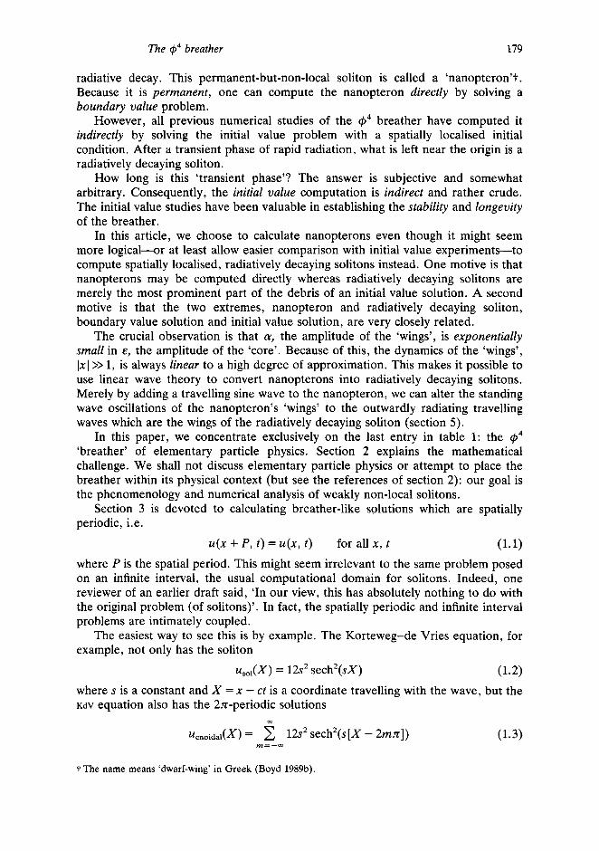
The 94 breather 179

radiative decay. This permanent-but-non-local soliton is called a ‘nanopteron’t. Because it is permanent, one can compute the nanopteron directly by solving a boundary value problem.

However, all previous numerical studies of the G4 breather have computed it indirectly by solving the initial value problem with a spatially localised initial condition. After a transient phase of rapid radiation, what is left near the origin is a radiatively decaying soliton.

How long is this ‘transient phase’? The answer is subjective and somewhat arbitrary. Consequently, the initial value computation is indirect and rather crude. The initial value studies have been valuable in establishing the stability and longevity of the breather.

In this article, we choose to calculate nanopterons even though it might seem more logical-or at least allow easier comparison with initial value experiments-to compute spatially localised, radiatively decaying solitons instead. One motive is that nanopterons may be computed directly whereas radiatively decaying solitons are merely the most prominent part of the debris of an initial value solution. A second motive is that the two extremes, nanopteron and radiatively decaying soliton, boundary value solution and initial value solution, are very closely related.

The crucial observation is that CY, the amplitude of the ‘wings’, is exponentially small in E, the amplitude of the ‘core’. Because of this, the dynamics of the ‘wings’, 1x1 >> 1, is always linear to a high degree of approximation. This makes it possible to use linear wave theory to convert nanopterons into radiatively decaying solitons. Merely by adding a travelling sine wave to the nanopteron, we can alter the standing wave oscillations of the nanopteron’s ‘wings’ to the outwardly radiating travelling waves which are the wings of the radiatively decaying soliton (section 5 ) .

In this paper, we concentrate exclusively on the last entry in table 1: the G4 ‘breather’ of elementary particle physics. Section 2 explains the mathematical challenge. We shall not discuss elementary particle physics or attempt to place the breather within its physical context (but see the references of section 2): our goal is the phenomenology and numerical analysis of weakly non-local solitons.

Section 3 is devoted to calculating breather-like solutions which are spatially periodic, i.e.

u(x + P, t ) = u(x, t ) for all x , t (1.1) where P is the spatial period. This might seem irrelevant to the same problem posed on an infinite interval, the usual computational domain for solitons. Indeed, one reviewer of an earlier draft said, ‘In our view, this has absolutely nothing to do with the original problem (of solitons)’. In fact, the spatially periodic and infinite interval problems are intimately coupled.

The easiest way to see this is by example. The Korteweg-de Vries equation, for example, not only has the soliton

uSol(X) = 12s2 sech2(sX) (1.2) where s is a constant and X = x - ct is a coordinate travelling with the wave, but the Kdv equation also has the 2n-periodic solutions

m

uCnoidal(X) = 12s’ sech2(s[X - 2mnl) (1.3) m=-m

t The name means ‘dwarf-wing’ in Greek (Boyd 1989b)

180 J P Boyd

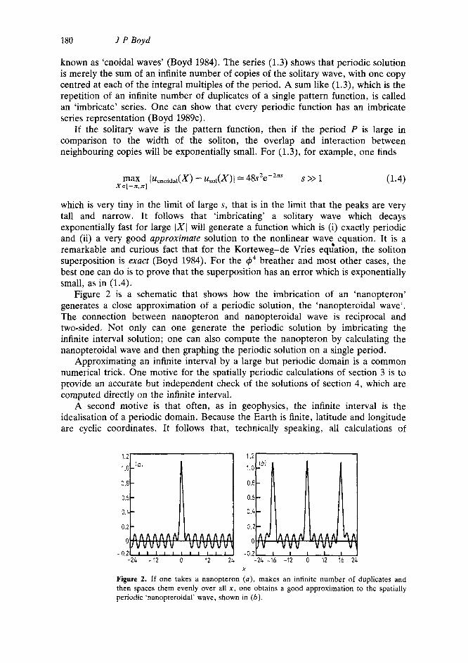
known as ‘cnoidal waves’ (Boyd 1984). The series (1.3) shows that periodic solution is merely the sum of an infinite number of copies of the solitary wave, with one copy centred at each of the integral multiples of the period. A sum like (1.3), which is the repetition of an infinite number of duplicates of a single pattern function, is called an ‘imbricate’ series. One can show that every periodic function has an imbricate series representation (Boyd 1989~).

If the solitary wave is the pattern function, then if the period P is large in comparison to the width of the soliton, the overlap and interaction between neighbouring copies will be exponentially small. For (1.3), for example, one finds

max (ucnoida,(X) - us,,,(X)l ̂ I 48s2e-2ns s >> 1 (1.4) x E[ -n, n]

which is very tiny in the limit of large s, that is in the limit that the peaks are very tall and narrow. It follows that ‘imbricating’ a solitary wave which decays exponentially fast for large 1x1 will generate a function which is (i) exactly periodic and (ii) a very good approximate solution to the nonlinear wave equation. It is a remarkable and curious fact that for the Korteweg-de Vries eqGation, the soliton superposition is exact (Boyd 1984). For the @ 4 breather and most other cases, the best one can do is to prove that the superposition has an error which is exponentially small, as in (1.4).

Figure 2 is a schematic that shows how the imbrication of an ‘nanopteron’ generates a close approximation of a periodic solution, the ‘nanopteroidal wave’. The connection between nanopteron and nanopteroidal wave is reciprocal and two-sided. Not only can one generate the periodic solution by imbricating the infinite interval solution; one can also compute the nanopteron by calculating the nanopteroidal wave and then graphing the periodic solution on a single period.

Approximating an infinite interval by a large but periodic domain is a common numerical trick. One motive for the spatially periodic calculations of section 3 is to provide an accurate but independent check of the solutions of section 4, which are computed directly on the infinite interval.

A second motive is that often, as in geophysics, the infinite interval is the idealisation of a periodic domain. Because the Earth is finite, latitude and longitude are cyclic coordinates. It follows that, technically speaking, all calculations of

1.21 1

-0.2- -24 -12 0 12 24

-0.21- -24 -16 -12 0 12 16 L

X

Figure 2. If one takes a nanopteron (a ) , makes an infinite number of duplicates and then spaces them evenly over all x., one obtains a good approximation to the spatially periodic ‘nanopteroidal’ wave, shown in (6) .

The 44 breather 181

oceanographic or meteorological solitary waves are really computations of extreme cnoidal waves instead (Boyd 1985).

Thus, nanopteroidal waves are intrinsically as interesing as nanopterons. In sections 3 and 4, we compute both species. The infinite interval calculations require a special trick because the oscillatory ‘wings’ wreck any conventional spectral or finite difference algorithm.

The oscillatory wings can be manipulated by adding in linear combinations of the eigenfunctions of the linearised wave equation. Section 5 computes these eigenfunc- tions and explains their role in enlarging the spectrum of breathers.

2. The tP4 breather: background

The quasisolitary waves of the G4 field theory have been extensively studied by previous investigators: Dashen et aE (1974), Kudryavtsev (1975), Getmanov (1976), Makhankov (1978), Sugiyama (1979), Moshir (1981), Campbell et al (1983), Campbell and Peyrard (1986), and Segur and Kruskal (1987) are but a partial list. The model is

@xx - @tt + @ - @3 = 0 (2.1) where subscript x or t denotes differentiation with respect to that coordinate. The ‘breathers’ oscillate about either @ = 1 or @ = -1, so it is convenient to make the change of variable

u = d T l (2.2)

U,, - ut, - 2u T 3u2 - u3 = 0 (2 * 3)

which gives the differential equation

(the @ 4 equation).

We shall choose the upper (negative) sign here, and study breathers that fluctuate about @ = 1. Segur and Kruskal (1987) choose the opposite, which gives a ‘minus’ breather that oscillates about -1. The difference is not significant because u(x, t ) for the ‘plus’ breather is merely the negative of the other solution.

The ‘breather’ solution of (2.3) is described to lowest order in E . by the perturbative approximation

u(x , t ) - (2/3)l”~ sech(Ex)cos(ot) + O(E’) (2.4) where the perturbative parameter E is defined (for all o, even when E(W) is not small) by

(2.5) & = (2 - o2)1/’.

We shall use o and E(O) interchangeably to parametrise the family of breather solutions. Through a trivial rescaling, one can generalise (2.4) to waves that translate at a steady speed as well as pulsate, but because the rescaling is so simple, we lose no generality for nanopterons by restricting attention to waves with zero phase speed. The term ‘breather’ is widely used to describe solitons which oscillate and translate with time (instead of merely translating with steady shape like Korteweg-de Vries solitons). It is conventional in the literature (Segur and Kruskal 1987) to apply this generic term to the @ 4 solutions that can be approximated by (2.4).

182 J P Boyd

The asymptotic expansion (2.4) and (2.5) is due to Dashen et a1 (1974), but the ‘breather’ or ‘bion’ was independently discovered in numerical oscillations of G4 kinks by Kudryavtsev (1975).

Almost from the beginning, it was suspected that (2.4) was only an asymptotic (as opposed to convergent) series. Part of the evidence was that numerical solutions radiatively decay by leaking energy to infinity. Another reason for doubting the convergence of (2.4) is a simple argument given by Eleonskii et a1 (1984).

If we expand a time-periodic breather in the Fourier series m

u(x , t ) = 2 An(x) cos(nwt) (2.6) n =O

direct substitution into (2.3) gives an infinite set of coupled ordinary differential equations for the time harmonics, {An@)}. If the breather is localised in the sense that u(x , t ) + 0 as Ix I + 00 for all t, then for sufficiently large x , the nonlinear terms in (2.3) are negligible. In this ‘far field’ limit, the differential equations for the A,(x) are linear and uncoupled:

An,xx + [n’w’- 2]An = 0 1x1 >> 1. (2.7) The constant in time and the fundamental decay exponentially with x in the breather frequency range, O < w2<2”’, but A2(x) and all the higher harmonics are oscillatory.

Thus, a solution which is a true solitary wave in the sense that u(x, t ) decays as IxJ+m is not possible ‘unless a miracle happens’. For the sine-Gordon equation, which is integrable and has an infinite number of conservation laws, the amplitude of all of the far field harmonics is zero, and true breathers exist. We cannot expect such miracles for non-integrable equations like the G4 model. However, Segur and Kruskal (1987) have shown that the perturbative formula (2.4) is a good approxima- tion to an extremely long-lived phenomenon by demonstrating that the amplitude of the far field radiation is exponentially small in the width parmeter E . Through clever use of matched asymptotic expansions in the complex x plane, they show that

Iu(x, t)l c 0.018e-3~8““ 1x1 >> 1, E << 1. (2.8) When E is sufficiently small, the radiative leakage to infinity is so weak that the decay timescale of the breather is longer than the predicted lifetime of the universe!

To put it another way, as done by Hunter and Scheurle (1988), non-local waves are not solitons in the classical sense, but they are ‘arbitrarily small perturbations of solitary waves’ in the sense that the wings can be made arbitrarily small in comparison with the core by taking the core amplitude to be sufficiently small.

3. Spatially periodic breathers

If we replace the infinite interval by the finite domain x E [-P/2, P/2] subject to boundary conditions of spatial periodicity,

u(x + P , t ) = u(x, t ) all x , t (3.1) where P is the period, then all the preceding arguments against the existence of a breather collapse. The solitary wave need not decay by radiative leakage to infinity because there is no infinity.

The iP4 breather 183

This removal of negative arguments is not the same as offering a positive existence proof that spatially periodic breathers exist. We are assuming that there are breathers which are simply periodic in both space and time. However, our numerical calculations, which are sufficiently accurate to resolve both the ‘core’ and the ‘wings’, are strong evidence that spatially periodic 44 breathers are real.

Since the perturbation series for the breather is symmetric in both time and space (with proper choice of the origin) (Segur and Kruskal 1987), it is sufficient to expand the breather as

M N

u(x , t ) = 2 2 amn cos(mkx) cos(nwt). m=O n=O

(In section 5, we shall make additional remarks about possible unsymmetric breathers.)

To cope with the nonlinearity, we use the Newton-Kantorovich iteration method. That is, we write

u(’+l)(x, t ) = u(‘)(x, t ) + 6‘“(x, t ) (3.3)

linearise (2.3) about the ith iterate, u(‘)(x, t ) , and neglect quadratic and higher powers of the correction, 6( ’ ) (x , t ) , to obtain

622 - 6:;) - (2 + 6u(’) + 3[~(’)]2)6(’) = -{U$; - U$) - 2u(’) - 3 [ u(i) 1 2 - [u(’)13>. (3.4)

This is solved by expanding both U(’) and 6( ‘ ) (x , t ) as double Fourier series like (3.2) and demanding that the left and right sides of (3.4) agree exactly at the ( N + 1)(M + 1) ‘collocation points’,

x k = n(2k + 1)/(2M + 2)

k = 0 , . . . , M ti = n(2j + 1)/(2N + 2)

j = O , . . . , N (3.5)

where the indices k and j vary independently, i.e. the two-dimensional array of points is the direct product of the one-dimensional arrays defined by (3.5). Equations (3.3) and (3.4) are iterated until 6( ’ ) (x , t ) is negligibly small.

The Fourier pseudospectral/Newton-Kantorovich algorithm is discussed in greater detail in Boyd (1986a, b) and Canuto et a1 (1987). For P = 28.9 and w = 1, which is the most numerically challenging case we ran, u(x, t ) for a 12 x 8 basis ( M = 11, N = 7) differed from that for a 15 X 10 truncation by only 0.006. Because of the ‘exponential convergence’ of spectral algorithms, the actual 15 x 10 error is probably considerably smaller than this difference.

The spatially periodic breathers are, for all sufficiently large periods P, strongly localised about the origin. Segur and Kruskal argue that the dominant radiation has the wavenumber

kz = (40’ - 2)”’ (3.6)

where A&) - 4vz cos(k,x + phase) for large 1x1 where vz is a constant. The numerical results confirm that this asymptotic radiation for the second time harmonic does indeed dominate the far field of u(x, t ) even for w as small as 1. Further, the radiation is always weak, regardless of P, for w 3 1.

However, the amplitude of the oscillatory ‘wings’ is sensitive to the spatial period

184 J P Boyd

modulo the wavelength of the dominant radiation,

When P is a half-integral multiple of W, that is P = ( r + 4)W where r is an integer, then

W 2~d/kz. (3.7)

u(x , t ) - a l ( w ) sin(k, 1x1) 1x1 >> 1 (3.8)

u(x, t ) - az(w) COS(k2X) 1x1 << 1 (3.9)

where al(o = 1) = 0.0271. When P is an integral multiple of W, then

where a2(w = 1) = 0.0107. When P is not an integral or half-integral multiple of W, the amplitude and phase of the radiation are intermediate, for w = 1, between the extremes given by (3.8) and (3.9). For higher frequencies, a ( P ) may achieve its maximum when P mod W is a fraction other than 4,

For all o, however, the solution in the far field is, for sufficiently large P, a function only of the fractional remainder when P was divided by W, that is

where int[q] denotes the largest integer s q . a (P) = a([P/W] - int[P/W]) P >> W (3.10)

X X

-0.051 I I I I I I I I I 1 0 2 4 6 0 10

X

Figure 3. Comparison of time harmonics ( a ) A&), ( b ) A,(n) and (c) A2(x) for o = 1 and the spatial period P = 5.5W (full curve), P = 6W (broken curve) and P = 6.5W (full curve) where W is the spatial period of the dominant radiation. Note that the curves for P = 5 . 5 W and 6.5W are visually indistinguishable in all three plots, justifying (3.10).

The $4 breather 185

The reason for this sensitivity is fairly obvious from figure 2: when nanopterons are superimposed to make the nanopteroidal wave, the wings of the central copy of the pattern function must match smoothly onto those of the copies of the nanopteron which are centred at x = f P where P is the spatial period. The fact that we can successfully make this match for all P at a given E suggests that when E (or equivalently, the frequency) is fixed, the spatially symmetric nanopteron still has one internal degree of freedom. In sections 4 and 5 , we shall confirm this supposition.

Figure 3 illustrates the extremes of the dependence on P for the three principal time harmonics for unit breather frequency. A&), the constant in time, is approximately independent of P . A , (x) is mildly sensitive to P, but the effect is so weak that one must have good eyes to detect it on the graph. A&) varies much more strongly with the spatial period, but mostly through the far field radiation.

As the frequency decreases below o, other runs not presented show that the strength of the asymptotic oscillation rapidly increases. At o = o, = (1/2)”’, the far field radiation of A&) makes a transition from exponential behaviour to oscillatory behaviour-but at this critical parameter value, the asymptotic solution for A2(x) is linear and therefore unbounded. Even for w = 0.8 (>a,), however, the radiation is so large that the notion of a weakly non-local quasisolitary wave is nonsense.

In consequence, we have somewhat arbitrarily chosen to present results for w a 1. The notion of the localised breather can be applied to slightly lower frequencies, too, but as the ratio of core amplitude to wing amplitude decreases rapidly with decreasing w, the concept of the quasisoliton becomes less and less meaningful.

X

Figure 4. The breather for five different times over one-half of a period. (Since the oscillation is symmetric about t = 0 , the plots for the second half of the cycle are identical to the curves shown here, but taken in reverse order.) The breather evolves from the uppermost graph to bottom curve and then back again over the course of a full cycle.

186 J P Boyd

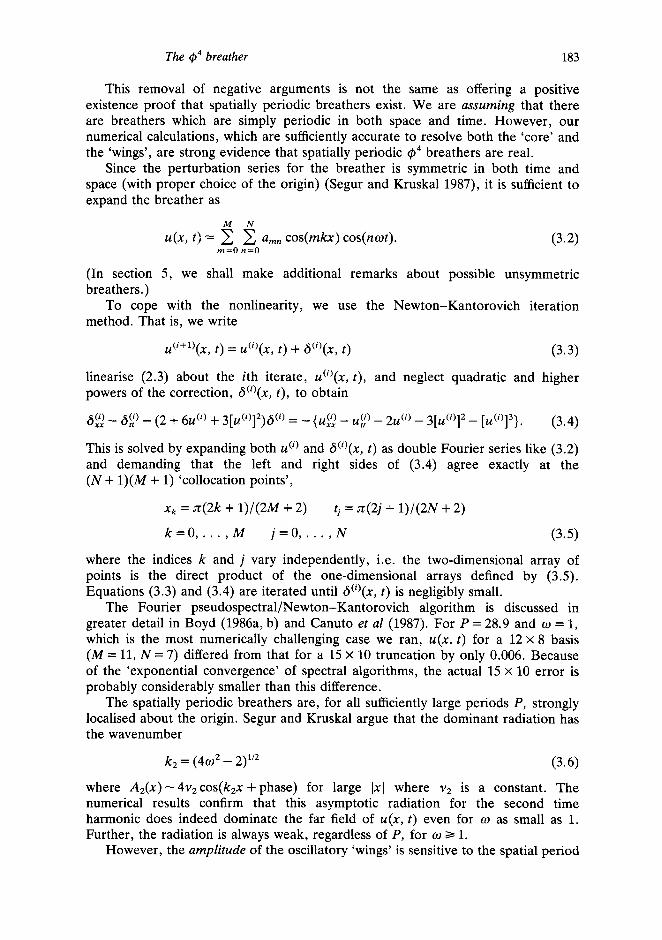
Figure 5. Perspective x-t plot of the 94 breather. Because u(x, t ) is symmetric about the origin in both space and time, only the quadrant x 3 0, t 3 n is illustrated.

Figures 4 and 5 illustrate the shape of the breather for w = 1. In contrast to the symmetrical, small amplitude oscillation for w = 2l’* which is accurately described by (2.4), the larger amplitude breather is highly asymmetric. The trough is much deeper than the peak, and the breather is negative for almost three quarters of each temporal period.

Kudryavtsev (1975), who created breathers by colliding kink solitons in a time-dependent numerical model, also observed this strong asymmetry. His figure 1 shows that his solutions, which oscillate about q5 = -1, have a much larger peak than a trough, and the breather is positive (negative for pulsations about q5 = 1, such as ours) for most of a period.

However, his maxima and minima-approximately 1.7 and -0.4 as measured from his graph-are impossible to reconcile with the numerical values we compute. Our figure 4 shows that when the trough is as deep as -0.55, the crest is only as large as 1.1 (reversing signs to agree with his sign convention).

It is possible that Kudryavtsev’s diagram is only a schematic. He in any event deserves full credit for independent discovery of the breather. However, it is obvious that computing breathers through time-dependent collisions, which super- imposes transient excitations on the basic pulsation, is a rather crude tool for studying the phenomenon. Computing the breather as the solution to a nonlinear eigenvalue problem is a far more direct and accurate methodology.

4. Numerical calculations on the infinite interval: the rational Chebyshev/radiation function pseudospectral method

Boyd (1989d, 1990) has developed a method for computing solutions on an infinite interval with far field radiation. The trick is to use a mixed spectral basis which is composed of the orthogonal rational functions of Boyd (1987) plus one or more ‘radiation functions’ which are chosen to mimic the asymptotic behaviour of U (x , t ) .

The 94 breather 187

Since the method is fully explained in Boyd (1989d, 1990), we shall omit the details and concentrate on the results.

One complication is that the breather is not unique. The linearised wave equation (3.4) has two eigenfunctions with zero eigenvalue. One may add arbitrary multiples of these eigenfunctions to any breather solution to obtain a new breather solution (with an error which is second order in the eigenfunction amplitudes). The calculation of these eigenfunctions is the theme of the next section. Here, it suffices to note that for a given frequency w, the infinite interval breathers form a two-parameter family. One may numerically calculate any of these infinite interval breathers by specifying the appropriate radiation function.

Segur and Kruskal’s choice is to demand exponential decay as x + --CO. This doubles the far field oscillation as X+-CO. It is only in this one-sided far field radiation, however, that their unsymmetric nanopteron differs from that calculated here.

Our choice is to ask the following question: which breather most closely resembles the result of an initial value experiment with a localised initial condition?

The answer may be cribbed from Boyd (1989d), or derived directly via trigonometric identities. All solutions to the Cp4 field equation that evolve from localised initial conditions, whether similar to the breather or not, have a far field which consists of outward-propagating radiation. All of the nanopterons calculated here and in the previous section are, strictly speaking, standing waves for 1x1 >> 1. However, we may convert the standing wave solution into one which has the desired outward propagation by adding the appropriate sine wave to the nanopteron.

In Boyd (1989d), this standing breather-cum-sine wave superposition is an exact solution because the wave equation of that earlier article is linear. Here, there are apparent problems.

Because the G4 equation is nonlinear, exact superposition is not possible. Furthermore, the linear solution of Boyd (1989d) had only a single sinusoidal component as 1x1 + -CO. The G4 breather has a countable infinity of waves for 1x1 >> 1, one with the wavenumber k, = (n202 - 2)”2 for each A , @ ) with n 2 plus the harmonics of this set which are created by their nonlinear interaction.

However, even for w as small as 1, the far field radiation is dominated by a single component with wavenumber k2 defined by (3.6), and even the amplitude of this wave, which we label as the ‘radiation coefficient’ a, is very small. Consequently, when we add an O(a) sinusoidal wave, the standing breather/sine wave sum will solve the full, nonlinear G4 equation with an error of only O(a2).

A more sophisticated procedure is to apply perturbation theory in powers of a to calculate the far field to as much accuracy as desired. This is done for non-local capillary-gravity solitons in Boyd (1989e). For our purposes, however, a linear approximation will suffice.

Boyd (1989d) shows that the constraint that the wave sum have outward propagation is sufficient to uniquely specify the nanopteron and demand that it asymptote to

a sin(k2x) cos(2wt) t ) - [ -a sin(+) cos(2ot)

x + -CO

x + - w (4.1)

for some coefficient a. We shall refer to the nanopteron with the asymptotic behaviour of (4.1) as the ‘standard breather’.

This solution may be reproduced in a spatially periodic calculation by choosing

188 J P Boyd

the period P to be an half -integral multiple of the wavelength of the dominant far field radiation. That is, P = ( r + 4) W where W = 2n/(4w2 - 2)l”.

On the infinite interval, the numerical method is to expand the nanopteron as M N

u(x, t ) = amn[TBzm(x) - 11 cos(nwt) + a tanh(&x) sin(k,x) cos(2ot) (4.2) m = l n=O

where k2 is defined by (3 .6) . To convert this standing wave into a solution with outward radiation away from the origin, we add

usine(x, t ) = a cos(k,x) sin(2ot). (4.3)

One may easily verify that the sum of the nanopteron plus uSine(x, t ) satisfies the G4 equation to within an error of O(a2), and that the sum describes outward-radiating waves in the far field. Thus, the numerical strategy for computing a radiatively decaying soliton is always to compute the nanopteron first-an exact, legitimate infinite interval solution that does not decay with time, albeit a non-local solution. Then, as a second independent step, we perform the approximate superposition of the nanopteron with uSine(x, t ) as defined by (4.3).

Table 2. Values of A2(x) as computed through different numerical methods. Column 2: Fourier cosine series, 15 x 10 basis. Column 3: TB,(x) series with one radiation function, 12 x 8 basis. Column 4: TB,(x) series with one radiation function, 15 x 10 basis. The strength of the dominant radiation for large x as determined from the oscillations of u(x) (column 2) or more directly from the coefficient of the radiation basis functions (columns 3,4), is also shown.

X

1 5 x 1 0 1 2 x 8 15 X 10 Fourier TB,/rad TB,/rad

0 0.389 0.778 1.166 1.555 1.944 2.333 2.721 3.110 3.499 3.888 4.276 4.665 5.054 5.443 5.831 6.220 6.609 6.998 7.386 7.775

Radiation coefficient

0.203 0.196 0.174 0.141 0.103 0.0639 0.0283 0.00054

-0.0167 - 0.0224 -0.0178 -0.00600

0.00840 0.0206 0.0268 0.0251 0.0160 0.00217

- 0.0123 - 0.023 1 -0.0271

0.0271

0.204 0.196 0.174 0.141 0.102 0.0627 0.0276 0.00066

-0.0157 -0.0209 -0.0164 -0.00521

0.00835 0.0198 0.0256 0.0239 0.0152 0.00190

-0.0120 -0.0223 - 0.0262

0.0262

0.203 0.196 0.174 0.141 0.103 0.0640 0.0284 0.00053

-0.0168 -0.0225 -0.0179 -0.00607

0.00838 0.0207 0.269 0.0252 0.0161 0.00218

-0.0124 -0.0233 -0.0273

0.0274

The $ J ~ breather 189

The pseudospectral procedure is to demand that the residual function defined by

The TB,(x) are the rational Chebyshev functions of Boyd (1987). The substituting u(x, t ) into (2.3) s!it>uld be zero at a set of collocation points.

interpolation points are the intersections of the lines defined by

x = x i = L COt(42i - 1]/(2M)) i = 1, . , . , M (4.4)

with the lines t=t i where the ti are given by (3.5). The map parameter L is (somewhat arbitrarily) chosen to equal 2 / ~ where E(W) is defined by (2.5).

The last term in (4.2) is the ‘radiation basis function’. Its form is chosen so as to give the desired far field radiation, which the rational Chebyshev functions cannot accurately approximate. Note that all the TB2,(x)-+ 1 in the limit 1x1 + 03 so that all the terms in (4.2) vanish for large x except the radiation function, which completely describes the far field in the numerical approximation.

In principle one could use many radiation functions, but because the asymptotic radiation is dominated by a single wave until the amplitude of the radiation is so large that the very concept of the breather becomes meaningless, we used only a single radiation function. Numerical experiments showed that the mixed TB,(x)/radiation function basis becomes ill-conditioned when many radiation functions are employed. Fortunately, this problem can be alleviated by using a least-squares procedure in which the number of interpolation points is larger than the number of unknowns. However, since one radiation function gave good results, we mention the possibility of using more such functions only in passing.

Table 2 is a comparison between the computed values for the coefficient of cos(2wt), A2(x) , as obtained through three different calculations. One used a Fourier basis on the periodic interval with 150 basis functions; the second and third employed the mixed TB,(x)/radiation basis on the infinite interval with two different truncations. The close agreement between this trio of calculations is gratifying.

In particular, the computed radiation coefficient CY agrees within 1.1% with the amplitude of the oscillations for large x on the periodic interval. The pseudospectral method with mixed basis has allowed us to compute the (standing) breather directly, without the clumsiness of an initial value calculation, even though the breather is only a quasisoliton, and has a small radiative ‘tail’ even for very large x .

Figure 6 is a comparison between computed values of CY and the matched asymptotics perturbation theory of Segur and Kruskal (1987). (To perform the comparison with Segur and Kruskal, it is necessary to use the superposition of a sine wave to convert their one-sided breather to a form identical to ours.)

Bender and Orszag (1978) offer many examples where singular perturbation theory is accurate even when the perturbation parameter E is small. In contrast, the perturbative radiation coefficient of Segur and Kruskal is at least an order of magnitude too small (note the logarithmic scale of figure 6) until CY<O.OOO~. In applications, whenever (Y and E are small enough so that the Segur-Kruskal formula is accurate, neglected effects like dissipation will probably be more important than the extremely weak radiation to infinity.

The range of accuracy for perturbation theory for capillary-gravity water waves is also very small (Boyd 1989e). It may be that this inaccuracy is a generic feature of non-local solitary waves. It is comforting, however, that the exponential dependence on E , exp(-3.85/~), is clearly supported by the graph: the numerical curve for CY(E) is asymptoting to a straight line on this logarithm-against-l/E plot.

190 J P Boyd

I / €

Figure 6. Log la) as a function of E where a is the radiation coefficient and where E = (2 - C U ~ ) ~ ’ ~ is the perturbation parameter. Full curve: mixed Chebyshev/radiation function pseudospectral computation with 495 (33 space X 15 time) basis functions. Broken curve: extrapolation of Segur and Kruskal’s (1987) matched asymptotics formula.

5. Eigenfunctions of the linearised wave equation

Each Newton-Kantorovich iteration solves the linearised wave equation (3.4). In the limit E + 0, this ‘Newtonian-Kantorovich equation’ collapses into the linear, constant coefficient far field equations. If one writes the solution to (3.4) as

m

6 ( x , t ) = 2 6, (x ) cos(not)

6,,& + [n”w” - 216, = . . .

(5.1)

(5.2)

n=O

then, with an error of O ( E ) , (3.4) is the uncoupled set of differential equations

where the ellipsis (. . .) represents the ntime harmonic of the residual of the wave equation. The inhomogeneous terms in (5.2) have been omitted because they are irrelevant to present purposes. What matters is that the homogeneous solutions of (5.2) are bounded for n 3 2, and thus are eigenfunctions of the operator in the Newton-Kantorovich equation (3.4). Explicitly, the eigenfunctions are

where e,,&) = cos(k,x) e,,&) = sin(knx) n 3 2 (5.3)

k, = (n’d - 2)’” ‘the far field wavenumber’. (5.4) Equations (5.3) and (5.4) suggest that for fixed frequency (or E ) , the breather is

an infinite-parameter family. As explained earlier, however, the far field of the breathers computed in sections 3 and 4 is dominated by a single component: that for n = 2. Consequently, the numerical scheme of section 4 only needs to make a choice within a two-parameter family.

The 44 breather 191

There are two approximations in (5.3) and (5.4). The first is that if p is the amplitude of one of the eigenfunctions, then adding the eigenfunction to the breather creates an error of O(p2). This error may be removed by the Newton- Kantorovich iteration after first modifying the radiation functions of section 4 to asymptote to the desired sum of the ‘standard breather’ defined by (4.1) and the eigenfunction (5.3).

The other error is that the Newton-Kantorovich equation is not really constant coefficient, but rather has variable coefficients. The varying parts of the coefficients are O(E) and are proportional to the breather or to the square of the breather. The same numerical methods used to compute the breather can be equally well applied to compute the eigenfunctions, too.

It is more illuminating, however, to calculate the eigenfunctions using a perturbation series in E. For simplicity, we shall give the result for only for e,,&; E), the symmetric eigenfunction for the second time harmonic. Almost all the difference between the two solutions shown in figure 3(c) is proportional to this eigenfunction.

There are two complications in the perturbation theory. First, even if the differential equation for were uncoupled from all the other equations in the set (5.2), it would still be necessary to solve this equation via the WKB method (Bender and Orszag 1978). That is, we write

6&; E) - p ( x ; E) cos(<P[x; E]) ( 5 . 5 ) where

- 6 K ( X ; E) dX‘

K ( X ; E) - k2 + O(e2) p(x; E) - 1 + O(E’) E << 1. (5.7)

The 0(1 ) eigensolution is given by (5.5) with k2 = 6l”; the corrections to K are determined at higher order.

The second complication is that the interaction of the breather with 6,(x) cos(2ot) will excite other harmonics in the eigenfunction. For example, if we write as before

u(x, t ) = A,(x) cos(not) n =O

where perturbation theory (Dashen et a1 1974) gives

A,@) - (2/3)l”~ sech(Ex) + O ( E ~ ) E << 1

A ~ ( x ) = -(3/4)Af + 0(&4)

Az(x) = (1/4)Af + 0(&4)

then at O(E)

6 1 , ~ ~ + [U2 - 2161 = 3~4162 63,xx + [9W2 - 2163 = 3~4162

since

(5.9a)

(5.9c)

(5.9b)

(5 . loa) (5. lob)

(5.11)

through an elementary trigonometric identity.

192 J P Boyd

It is not necessary to solve the first-order equations through WKB techniques because the inhomogeneous terms oscillate with a wavelength different from that of the homogeneous solutions for dl , d3. There are three additional simplifications. First, one may replace w’ in (5.10) by 2 with an error of O(E’); this replacement is consistent with the O(E) accuracy of (5.10). Second, because A1(Ex) varies only on the ‘slow’ O(E) length scale, one may treat this factor as a constant multiplying the rapidly varying factor a2. Third,

- -662 + O(E’). (5.12)

We thus obtain approximately

( 5 . 1 3 ~ ) (5.13b)

( 5 . 1 4 ~ ) (5.14b) ( 5 . 1 4 ~ ) (5.14d)

where

d2 - exp[(7/5)(2/3)l” sech(~x)]x(x; E)-’” cos( 6 K ( x ‘ ; E) dx’) (5.15)

where K ( X ; E) = (6 - 4 2 + 2 ~ ’ sech2(Ex)}1/2

where we have used perturbative relation

w’( E) - 2 - E2

(5.16)

(5.17)

and where the exponential in (5.15) is the result of a simple transformation to suppress the first derivative in the equation for a2 (Carrier and Pearson 1968) so that the standard WKB formula can be applied (Bender and Orszag 1978).

The perturbative approximation is a little complicated. It does show that the much simpler approximation

e2,&) - c o ~ ( 6 ~ ’ ’ x ) + O(E) (5.18)

can be consistently extended to higher order. Figure 3, which compares two different nonlinear numerical solutions for the same frequency, is another confirma- tion of the existence and relevance of this particular eigenfunction of the Newton-Kantorovich equation. As noted earlier, the difference between these two solutions is approximately proportional to e’,&).

It is the replacement of the classical soliton condition u(x)+O as 1x14 00 by the weaker condition of boundedness that allows these eigenfunctions. Because of their existence, weakly non-local solitons are a much broader family of solutions than analogous classical solitons. For example, the breather of the sine-Gordon equation is a one-parameter family, depending only on E or, equivalently, upon the frequency w. In contrast, we have shown that the @ 4 breather is at least a two-parameter family where the second parameter is the amplitude of e’,&).

The 9‘ breather 193

We must be content with the vague phrase ‘at least two-parameter’ because we have not performed numerical calculations of unsymmetric breathers, such as would be produced by adding a multiple of e2,Jx) , an antisymmetric eigenfunction, to a symmetric breather. Boyd (1989e) shows that even for the simpler case of capillary-gravity waves, computing antisymmetric non-local solitons is tricky. A full resolution of the issue of non-symmetric @ 4 breathers must be left for the future.

One final comment: when the period P of the nanopteron requires a far field phase that matches that of an eigenfunction, the amplitude of the ‘wings’ becomes large. Because this resonance occurs only for a discrete set of periods, one value of P in each interval of length W, we shall note this phenomenon only in passing. However, Boyd (1989e) illustrates this eigenfunction resonance in some detail.

6 . Summary

After a decade of studies of the 44 breather, it is gratifying to at least be able to directly calculate the breather by solving a nonlinear eigenvalue problem. (There have been many indirect calculations, that is solutions of the initial value problem, as reviewed by Campbell and Peyrard (1986).) It is also encouraging to escape the limitations of perturbation theory. The recent work of Segur and Kruskal (1987) has extended the &-power series of Dashen et a1 (1974) so as to calculate the radiation coefficient for small amplitude as given by (2.8). However, for E - 0(1), even this refined perturbation theory fails wretchedly. Comparison of the last line of table 1 with (2.8) shows that for E = w = 1, the Segur-Kruskal radiation coefficient is too small by a factor of 70. Both the Fourier and mixed rational Chebyshev/radiation basis, however, compute a accurately.

The concept of a solitary wave is so useful that there is great interest in applying it even when the solution is not strictly local, but instead has a small radiative tail that extends indefinitely far from the maximum of the disturbance. The far field radiation implies that such quasisolitary waves (including the @ 4 breather) will decay in time through radiation to infinity even in the absence of dissipation. However, in the real world there is always damping of some kind, and even when a solitary wave is strictly localised, it must decay. In applications, the distinction between soliton and quasisoliton is only one of spatial asymptotic behaviour, not of either decay with time nor of conceptual usefulness. Boyd (1989b,c) are good reviews of such ‘weakly non-local solitary waves’.

To turn from quasisolitons in general to the @4 breather in particular, we find that as the pulsation narrows, its amplitude increases, its frequency decreases, and the positive and negative phases of the oscillation become increasingly unbalanced and asymmetric. For w = 1, the maxima in U is only about half the magnitude of the minima. Clearly, the breather of this frequency, which corresponds to E = 1, is greatly distorted from the small amplitude breather. When E << 1, the perturbative approximation (2.4) shows that the maxima and minima are of equal size and the breather is symmetric in time. Even when E = 1, however, the amplitude of the far field oscillations is only 1/40 of the ‘core’ of the breather. The concept of the solitary wave is still useful.

Several needs remain. One is rigorous existence proofs for nanopterons that are simply periodic in time and for nanopteroidal waves that are both spatially and temporally periodic. Another is a proof or counter-proof for unsymmetric nanop-

194 J P Boyd

terons: are they non-existent unless one allows an O(a’) residual? A third is for time-dependent calculations in which the initial condition is a nanopteron with its wings removed. Presumably the only evolution would be the propagation of O(a) radiation to the left and the right from a large amplitude core that is a steady oscillation with logorithmic time decay (Boyd 1988, Segur and Kruskal 1987), but it would be satisfying to actually see this. We have made much progress in understanding non-local solitary waves, but the conclusions described above are based not on rigorous mathematics, but rather on very accurate and sophisticated numerical calculations.

Acknowledgments

This work was supported by the National Science Foundation through Grants 0CE8509923, OCE8800123 and DMS8716766. I thank Professor Harvey Segur for helpful preprints. I thank Elsevier for permission to reprints figures 1 and 2 from Boyd (1989a) and Academic Press for permission to reprint figures 5 and 6. I am appreciative of the reviewers for helpful comments.

References

Ablowitz M J and Segur H 1981 Solitons and the Inverse Scattering Transform (Philadelphia, PA:

Bender C M and Orszag S A Advanced Mathematical Methods for Scientists and Engineers (New York:

Boyd J P 1984 Cnoidal waves as exact sums of repeated solitary waves: new series for elliptic functions

- 1985 Equatorial solitary waves. Part 3: Westward-travelling modons J . Phys. Oceanogr. 15 46-54 ._ 1986a Solitons from sine waves: analytical and numerical methods for non-integrable solitary and

- 1986b An analytical & numerical study of the two-dimensional Bratu equation J . Sci. Comput. 1

- 1987 Spectral methods using rational basis functions on an infinite interval J . Comput. Phys. 69

- 1988 An analytical solution for a nonlinear differential equation with logarithmic decay Adv. Appl.

- 1989a Non-local equatorial solitary waves MesoscalelSynoptic Coherent Structures in Geophysical

SIAM)

Wiley)

SIAM J . Appl. Math. 44 952-5

cnoidal waves Physica 21D 227-46

183-206

112-42

Math. 9 358-63

Turbulence: Proc. 20th Liege Coli. on Hydrodynamics ed J C J Nihoul and B M Jamart (Amsterdam: Elsevier) pp 103-112

_. 1989b Weakly non-local solitary waves Nonlinear Topics in Ocean Physics: Proceedings of the Fermi Schooled A R Osborne and L Bergamasco (Amsterdam: North-Holland) in press - 1989c New directions in solitons and nonlinear periodic waves: Polycnoidal waves, imbricated

solitons, weakly non-local solitary waves and numerical boundary value algorithms Advances in Applied Mechanics ed T Y Wu and J W Hutchinson (New York: Academic) p 1 - 1989d A comparison of numerical and analytical methods for the reduced wave equation with

multiple spatial scales J . Comput. Phys. submitted - 1989e Weakly non-local solitons for capillary-gravity waves: the fifth-degree Korteweg-de Vries

equation Physica D submitted - 1990 A Chebyshev/radiation function pseudospectral method for wave scattering Comput. Phys. 4

in press Campbell D K and Peyrard M 1986 Physica 18D 47 Campbell D K, Schonfeld J F and Wingate C A 1983 Physica 9D 1 Canuto C, Hussaini M Y, Quarteroni A and Zang T A 1987 Spectral Methods in Fluid Dynamics (Berlin:

Springer)

The G4 breather 195

Carrier G F and Pearson C E 1968 Ordinary Differential Equations (Waltham, MA: Blaisdell) p 20 Combescot R, Dombre T, Hakim V, Pomeau Y and Pumir A 1986 Phys. Rev. Lett. 56 2036-9 Dashen R F, Hasslacher B and Neveu A 1974 Phys. Rev. D 10 4130 Eleonskii V M et a1 1984 Teor. Mat. Fiz. 60 395 Getmanov B S 1976 JETP Lett. 24 291 Hong D C and Langer J S 1986 Analytic theory of the selection mechanism in the Saffman-Taylor

problem Phys Rev Lett. 56 2032-5 Hunter J K and Scheurle J 1988 Existence of perturbed solitary wave solutions to a model equation for

water waves Physica 32D 253-68 Kudryavtsev A E 1975 JETP Lett. 22 82 Lorenz E N and Krishnamurthy V 1987 J . Amos. Sci. 2940-50 Makhankov V G 1978 Phys. Rep. 35C 1 McWilliams J C 1982 Proc. 91h US Nut. Congr. of Applied Mechanics (New York: American Society

Meiss J D and Horton W 1983 Solitary drift waves in the presence of magnetic shear Phys. Fluids 26

Moshir M 1981 Nucl. Phys. B 185 318 Pomeau Y, Ramani A and Grammaticos B 1988 Structural stability of the Korteweg-de Vries solitons

under a singular perturbation Physica 31D 127-34 Segur H and Kruskal M D 1987 Phys. Rev. Lett. 58 747 Sugiyama T 1979 Prog. Theor. Phys. 61 1550

of Mechanical Engineers)

990-7