A novel solution in the simultaneous deep optimization …journals.tubitak.gov.tr/elektrik/issues/elk-18-26-2/elk-26-2-10... · algorithm, with a numerical ... {Marquardt algorithm

Turk J Elec Eng & Comp Sci

(2018) 26: 743 – 754

c⃝ TUBITAK

doi:10.3906/elk-1706-250

Turkish Journal of Electrical Engineering & Computer Sciences

http :// journa l s . tub i tak .gov . t r/e lektr ik/

Research Article

A novel solution in the simultaneous deep optimization of RGB-D camera

calibration parameters using metaheuristic algorithms

Amir SAFAEI1, Saeid FAZLI2,∗1Department of Electrical Engineering, Faculty of Engineering, University of Zanjan, Zanjan, Iran

2Research Institute of Modern Biological Techniques, University of Zanjan, Zanjan, Iran

Received: 21.06.2017 • Accepted/Published Online: 15.11.2017 • Final Version: 30.03.2018

Abstract: This article presents a novel method for estimating 19 parameters of RGB and depth camera calibration

simultaneously. The proposed algorithm is based on applying metaheuristic methods for deep optimization and estimating

all parameters of intrinsic, extrinsic, and lens distortions of cameras. This paper compares four metaheuristic algorithms,

i.e. a genetic algorithm, particle swarm optimization, the colonial competitive algorithm, and the shuffled frog leaping

algorithm, with a numerical algorithm called singular value decomposition. The proposed method does not need the

initial estimation for optimization and it can avoid being trapped in local minima. By using nondirect estimation, we

achieve middle computing matrices such as the homography matrix, which is used in the pinhole camera model. Both

versions of Kinect sensors are used for the experimental evaluation. The mean square of the reprojection error criteria is

defined as the objective function in the proposed algorithm. The experimental results show that the proposed method

is more efficient and accurate than traditional numerical solutions.

Key words: Colonial competitive algorithm, homography, Kinect calibration, metaheuristic algorithm, radial lens

distortion, shuffled frog leaping algorithm

1. Introduction

The aim of camera calibration is the extraction of intrinsic and extrinsic parameters and the estimation of

radial and tangential lens distortions. In a calibration problem, the usage of projection equations should

relate 3D world coordinates to 2D image coordinates. This projection in a pinhole camera is modeled by

the homography matrix. Many methods have been proposed for camera calibration and the selection criteria

depend on environmental parameters, accuracy, and equipment. We used a simple plane grid of a checkerboard

based on the Zhang method [1] that is observed in at least three orientations. In this method, the homography

matrix should be estimated and it would be the base matrix for the subsequent steps of finding intrinsic and

extrinsic parameters. The traditional literature uses the least-square method for solving equations. Owing to

the statistical bias of this method [2,3], Kanatani proposed a renormalized maximum likelihood estimation [4].

Evolutionary algorithms have been proposed for solving calibration equations. The selection of these

methods depends on the essence of the equations. In the calibration problem, both local and global searches

are important, and this paper proposes a comparative solution through metaheuristic and numerical methods.

In the Zhang method [1], the Levenberg–Marquardt algorithm for solving equations was proposed. This

algorithm searches for a local minimum and not necessarily a global one. Hartley et al. [5] proposed a

∗Correspondence: [email protected]

743

SAFAEI and FAZLI/Turk J Elec Eng & Comp Sci

noniterative method called direct linear transformation. This method uses the total least squares computation

of the linear system of equations. Harker et al. [6] proposed a new noniterative solution based on the error

structure of the estimation matrix. They combined the forward H and reverse G projections to eliminate the

systematic bias of estimation. Herrera et al. [7] proposed a new technique for the simultaneous calibration

of two color cameras, with conjunction of a depth camera, and the relative pose between them. They used

Kinect as a depth sensor. Raposo et al. [8] improved the method of Herrera et al. [7] by decreasing the number

of images in the dataset (about 6–10 image-disparity pairs of the model plane). They also used the Kinect

sensor for the experiment and compared their results with the two versions of the Herrera method. Ji et al.

[9] used a genetic algorithm (GA) for camera calibration and proved that their method works with a minimum

number of control points. They showed that the GA method does not need an initial guess and their results

were improved in convergence, accuracy, and robustness. Another GA method, proposed by Hati et al. [10],

determines two rotational and three translational parameters. Song et al. [11] used particle swarm optimization

(PSO) on synthetic and real images for camera calibration. They used 35 sample points on the calibration box

but assumed that the cell shape of the CCD camera is square; therefore, the skewness of the intrinsic matrix

was assumed to be zero. Merras et al. [12] proposed an improved GA for camera calibration with varying

parameters. They compared their results with Tsai’s [13] method on synthetic and real data. Yilmaz et al.

[14] proposed external calibration parameters between stereo and Kinect sensors and used these parameters to

compensate for misalignments in 3D reconstruction. A thorough survey on the Kinect sensor was presented by

Han et al. [15].

In this paper, we use iterative metaheuristic methods for the estimation of all camera calibration param-

eters. The simulation of the proposed method has been accomplished on the Zhang dataset [1]. This dataset

provides a text file with each image to test the efficiency of the calibration algorithm independently of the corner

detection method that is applied in checkerboard images. In the next section, modeling between the 3D world

plane and its projected 2D image with the extraction of intrinsic, extrinsic, and lens distortions is discussed.

Section 3 describes the proposed method. In Section 4, the simulation results are shown and analyzed. In

Section 5, the experimental results with both versions of Kinect sensors are discussed and the undistortion of

the captured images is shown. Finally, the conclusion of this research is presented.

2. Projection of model plane into image plane

Based on the calibration object, the camera calibration can be divided into three groups: 3D reference objects,

2D plane-based objects, and 1D line objects. Other methods such as self-calibration, vanishing points for

orthogonal directions, and calibration from pure rotation have been suggested in some papers [16]. In this

paper, we use the second category for the calibration procedure and the modeling of projection is described as

follows.

2.1. Plane projection

A 3D point in world coordinates or the coordinate system of the scene (CSS), its correspondence in the

camera coordinate system (CCS), and its 2D projection in the image plane is denoted by M=[X ,Y ,Z ]T ,

MC=[XC ,YC ,ZC ]T , and m=[u ,v ]T , respectively. Based on the Zhang method [1], a 2D plane-based object

is used, and by assuming Z=0 for the model plane in the 3D world coordinates, we have M=[X ,Y ,0]T . By

adding a one as the last row of each vector, we show the augmented vectors as:

744


M = [X,Y, 0, 1]T , (1)

m = [u, v, 1]T . (2)

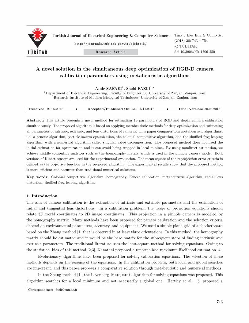
As shown in Figure 1, from the pinhole camera model, the projection of the 3D point to the image plane is

given by:

M[X,Y,Z] T

m[u,v]T

CCS

θ α

β

CSSc[u0,v0]T

Optical Axis

Figure 1. Pinhole camera model.

sm = A[R t]M, (3)

where s is an arbitrary scaling factor, A is the camera intrinsic matrix, R and t are respectively the rotation

and translation matrices, and the combination of [R t ] gives the extrinsic matrix. If [ r1 r2 r3 ] denotes the

columns of the rotation matrix R , because of Z=0 we can rewrite Eq. (3) as follows:

sm = A[ r1 r2 r3 t ]

X

Y

0

1

= A[ r1 r2 t ]

X

Y

1

. (4)

The model point M and its projection point m can be related to each other by:

sm = HM, (5)

where H = A[ r1 r2 t ] is a 3 × 3 matrix called the homography matrix, and, since Z=0, the model point

is shown by M = [X,Y, 1]T .

2.2. Orthonormality of the homography matrix

By denoting the columns of the homography matrix as [ h1 h2 h3 ] , we have:[h1 h2 h3

]= λA[ r1 r2 t ], (6)

where λ is an arbitrary scalar. Because of the orthonormality of r1 and r2 , ⟨r1, r2⟩ = 0 and ⟨r1, r1⟩ = ⟨r2, r2⟩ :

hT1 (A

−1)TA−1h2 = 0

hT1 (A

−1)TA−1h1 = hT2 (A

−1)TA−1h2

. (7)

Before solving Eq. (7), determining the homography elements is essential.

745


2.3. Extraction of equations system

Using Eq. (5), expanding the matrix format, we have:

u =h11X + h12Y + h13

h31X + h32Y + h33, v =

h21X + h22Y + h23

h31X + h32Y + h33, s = h31X + h32Y + h33. (8)

Rewriting this in the matrix format:

[X Y 1 0 0 0 −uX −uY −u

0 0 0 X Y 1 −vX −vY −v

]h11

h12

...

h33

= 0. (9)

Eq. (9) is in the form Lx=0, where L is a 2n× 9 matrix. Here, n denotes the point pairs in the model plane

and image. At least five independent points for solving Eq. (9) are required. After the determination of the

homography matrix, it is possible to find the intrinsic parameters by defining the B matrix as follows:

B = A−1A. (10)

The B matrix is symmetric. Thus, it is replaced by vector b with six degrees of freedom (DOF):

b =[B11 B12 B22 B13 B23 B33

]. (11)

If we assume that hi is the ith column of H , from Eq. (7) we have:

hTi Bhj = vTijb, (12)

vij = [hi1hj1, hi1hj2 + hi2hj1, hi2hj2, hi3hj1 + hi1hj3, hi3hj2 + hi2hj3, hi3hj3]T. (13)

By rewriting Eq. (7) in terms of v : [vT12

(v11 − v22)T

]b = 0. (14)

Eq. (14), similar to Eq. (9), is in the form Vb=0, with the difference being that the V matrix has 2n× 6

dimensions, where n is the number of image plane observations. Eq. (9) and Eq. (14) are nonlinear equations

that can be solved using metaheuristic methods. After solving Eq. (14), the intrinsic and extrinsic parameters

can be obtained as described in the Zhang method [1].

2.4. Lens distortion

Lens distortion is divided into radial and tangential distortions. In many cases, tangential distortion is small

and tends to be ignored. However, the first two terms of radial distortions are considered. By assuming (u, v)

and (x, y) as the ideal pixel image and normalized ideal pixel image, and (u′, v′) and (x′, y′) as the real pixel

image and normalized real pixel image, respectively, we have:{u′ = u+ (u− u0)[k1(x

2 + y2) + k2(x2 + y2)2]

v′ = v + (v − v0)[k1(x2 + y2) + k2(x

2 + y2)2], (15)

746


where k1 and k2 are the desired first two radial lens distortions. Eq. (16) is in the matrix format of Eq. (15).

Using n points in m images, we have 2mn equations:[(u− u0)(x

2 + y2) (u− u0)(x2 + y2)2

(v − v0)(x2 + y2) (v − v0)(x

2 + y2)2

][k1

k2

]=

[u′ − u

v′ − v

]. (16)

Eq. (16) is in the form Dk=d and, with matrix manipulation, we can find the k vector as:

DTDk = DT d ⇒ k =(DTD

)−1DTDd, (17)

where T is the matrix transpose operator. In the work of Drap et al. [17], a polynomial model for the calculation

of inverse radial lens distortion was presented.

3. Proposed method

Eq. (9) and Eq. (14) are the bottlenecks of the calibration procedure. The accuracy of the solutions may

influence the precision of intrinsic, extrinsic, and lens distortion parameters. In this paper, metaheuristic

methods are used for optimizing these equations and compared with the SVD method. The proposed method

has been examined with four metaheuristic algorithms: the GA [18], PSO [19], colonial competitive algorithm

(CCA) [20], and shuffled frog leaping algorithm (SFLA) [21]. Figure 2 shows the block diagram of the proposed

algorithm.

As shown in Figure 2, the evolutionary algorithms are used in two steps of the calibration procedure.

The stop criteria and cost function of these algorithms are similar to each other. The output of the proposed

algorithm is compared with the Zhang method [1] and the numerical SVD solution. The data provided online

by Zhang [1] are for researchers to test their algorithms without the influence of edge or corner extraction

methods. This reference dataset includes five different views of the checkerboard, five text files of extracted

corners corresponding to these images, and finally a text file of the corners of a model checkerboard. The

Levenberg–Marquardt (LM) method has been proposed for minimization in the Zhang method [1].

3.1. Cost function

The aim of an evolutionary algorithm is the optimization of a cost function. In this paper, there is a unique

cost function for the four proposed metaheuristic algorithms. This function is defined as the mean square of

the reprojection error. Both Eq. (9) and Eq. (14) are in the form of the homogeneous equation Lx=0. The

cost function is defined as follows:

error = Lx ⇒ Cost = mean(error2), (18)

where x is a vector of nine and six elements in Eq. (9) and Eq. (14), respectively. In each evaluation of the

cost function, a matrix of the whole population is assessed. The output of the cost function is a vector of the

mean squared error.

3.2. Comparison of methods

The main indicator of calibration precision is the reprojection error. This error can explain to what extent the

estimated parameters can correct the distorted captured images towards the ideal model plane. The reprojection

747


Metaheuristic algorithms

Feature point extraction (Corner Extraction of checkerboard)

Normalization

Homography matrix generation

LM [1] SVD GA PSO CCA SFLA

Homography matrix estimation

Eq. (14) matrix generation


LM [1] SVD GA PSO CCA SFLA

Intrinsic and extrinsic matrix generation

Intrinsic and extrinsic arameters estimation

Lens distortion arameters estimation

p

p

Figure 2. Block diagram of proposed algorithm.

error is defined as follows:

reprojection error =∥∥∥m−HM

∥∥∥ =∥∥∥m−A

[R t

]M

∥∥∥ . (19)

The average error for each image i is the mean of the reprojection error:

average errori = mean(∥∥∥m−HM

∥∥∥) . (20)

The total error is defined as the sum of the average errors over the captured images:

total error =

numof images∑i=1

average errori. (21)

The lens distortions include radial and tangential parameters. In most cases, the tangential parameters are

ignored [1], and only the first and second terms of the radial distortions are significant. These two parameters

are determined using Eq. (17).

4. Simulation of the dataset

As mentioned in Section 3, the dataset provided in Zhang’s paper [1] is used for simulation. The only difference

in each simulation is the procedure of parameter estimation. All the simulation results are compared with

748


unique assessment criteria. The outputs of the numerical and metaheuristic methods are compared with the

output of the Zhang method that is provided for researchers [1]. Table 1 shows the simulation results of the

proposed method.

Table 1. Intrinsic and lens distortion parameters of dataset of Zhang [1].

LM [1] SVDMetaheuristic algorithms

GA PSO CCA SFLA

A

α 832.5 866.0634 882.0014 865.7457 863.5523 860.0798

β 832.53 866.0468 880.6514 865.7397 863.5448 859.8971

γ 0.2045 0.1502 0.5298 0.1616 -0.0746 -0.5107

u0 303.959 301.1543 295.9408 301.0816 301.4531 296.9451

v0 206.585 219.5432 222.0691 219.6324 218.9486 215.8660

kk1 -0.228 0.0137 0.0127 0.0137 0.0137 0.0131

k2 0.190 -0.0195 -0.0186 -0.0195 -0.0195 -0.0191

Average error of

Image 1 2.5702 1.0653 1.4394 1.0632 1.068 1.0527

extrinsic parameters

Image 2 2.7144 1.0637 1.1677 1.0641 1.0599 1.1182

Image 3 2.279 1.0192 1.0747 1.0195 1.019 1.1627

Image 4 2.2053 0.89668 0.90741 0.8971 0.89528 0.9241

Image 5 1.6671 0.6609 0.66373 0.66068 0.66064 0.66933

Total error 11.4362 4.7058 5.2531 4.7045 4.7027 4.9271

4.1. Smoothness of convergence trace

One the main challenges of using metaheuristic algorithms is the smoothness of the convergence trace. Figures

3 and 4 show the smoothness of the convergence trace for both minimum cost and average cost in the

semilogarithmic plot, respectively.

0 100 200 300 400 500 600 700 800 900 1000

Iteration

10-8

10-6

10-4

10-2

100

Min

imu

m c

ost

GA

PSO

CCA

SFLA

0 100 200 300 400 500 600 700 800 900 1000

Iteration

10-9

10-8

10-7

10-6

10-5

10-4

10-3

10-2

Min

imu

m c

ost

GA

PSO

CCA

SFLA

Figure 3. Comparison of convergence trend in homogra-

phy matrix for estimation for fifth image of dataset.

Figure 4. Comparison of convergence trend in Eq. (14)

for estimation for fifth image of dataset.

749


In both Figures 3 and 4, the GA and PSO methods have faster convergence trends than the CCA and

the SFLA. By continuing the iteration, there is no significant change in the GA and PSO methods, but the

CCA and the SFLA reached better cost function values.

As shown in Figure 4, the minimum cost of the SFLA method is less than that of the CCA method, but

the total error of the CCA method is less than that of the SFLA (Table 1). This is due to the effect of the

precision of the homography parameter estimation in the previous step, as shown in Figure 5, hierarchically.

Intrinsic Parameters

Normalization

Extrinsic Parameters

Lens Distortion Parameters


egamI RI egamI BGR egamI RI egamI BGR

Kinect V1 Kinect V2

Homography

Solve Eq. (14)

Figure 5. Flow diagram of calibration procedure.

5. Experimental results

In this section, two versions of the Kinect sensor, V1 and V2, are used for the estimation of calibration

parameters. Both color and IR cameras are used in this experiment. We show one scene to both cameras

of each Kinect sensor and take one snapshot from each camera. Since the IR stream of Kinect V1 is defined in

the same RGB stream, it is not possible to take these streams simultaneously. The software program switches

between these streams after taking any snapshot from Kinect V1. This problem is solved by the Kinect V2

SDK, and it is possible to take these streams simultaneously.

In both case studies, each Kinect sensor captures eight scenes and tries to fill the whole frame by

checkerboard to figure out the lens distortions accurately and precisely. Figures 6 and 7 show images from

Kinect V1 and V2, respectively. It should be noted that the color camera of Kinect V2 has a wider width

than its IR camera. Moreover, because of the difference in the physical position of the color and IR cameras in

both versions of the Kinect sensors, there is a pure translation between the RGB and IR images in each set of

snapshots. For the homography estimation, the reprojection error criteria are used as the goal functions that

should be minimized by the proposed algorithm.

5.1. Case study 1

In this experiment, Kinect V1 is used for the study. The calibration parameters are compared with the results

of Karan [22]. Table 2 shows the calculated values of the calibration parameters. Since the extrinsic parameters

depend on the orientation and translation of the checkerboard, these parameters are not compared. Also, in

750


Figure 6. Images captured by Kinect V1: (top) color images, (bottom) IR images.

Figure 7. Images captured by Kinect V2: (top) color images, (bottom) IR images.

many cases, the Kinect sensor has various resolutions with different frame speeds. The RGB camera can provide

both resolutions of 1280 × 960 at 12 fps and 640 × 480 at 30 fps. The maximum resolution of the IR camera

is 640 × 480 at 30 fps. In many applications of this sensor, the 640 × 480 resolution of the RGB camera is

therefore used because of the alignment of the depth image and compatibility with the frame speed of the IR

camera. The difference of values in lens distortion and other parameters with the same resolution is caused

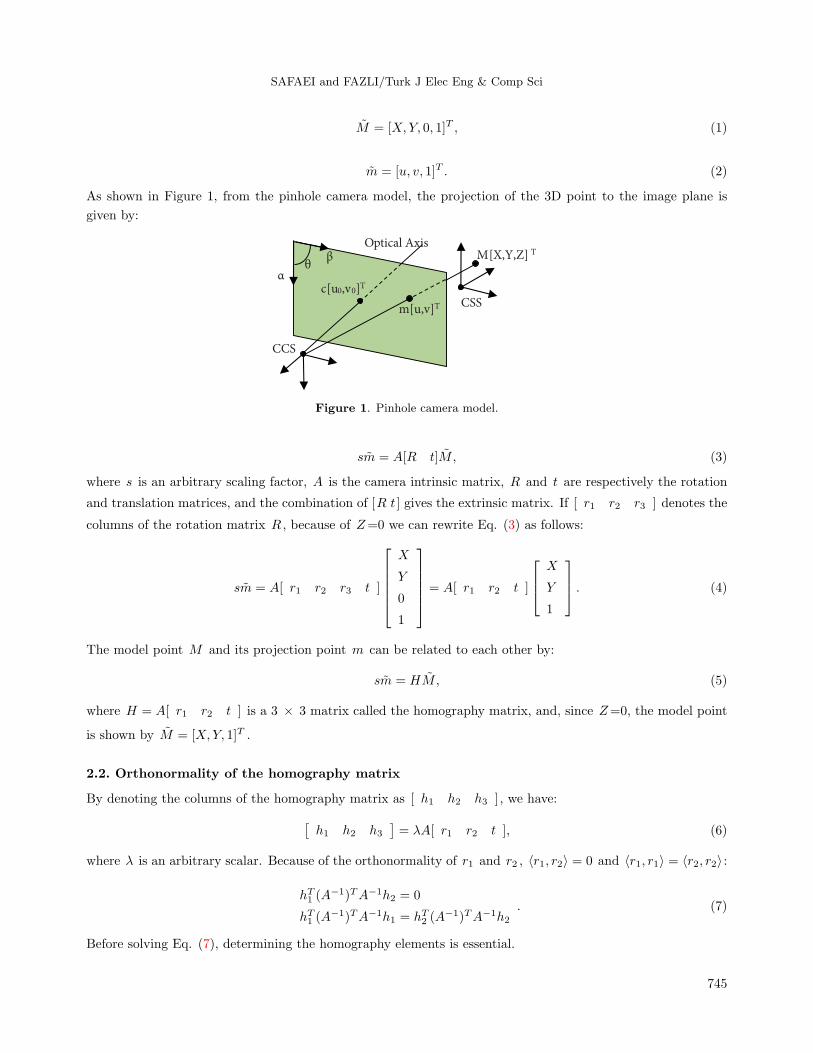
by the manufacturing process. Figure 8 shows the contour map of the radial lens distortion of the Kinect V1sensor.

5.2. Case study 2

This case study uses Kinect V2 for measuring calibration parameters. The differences between these two versions

of Kinect sensors were discussed in a few studies [23]. Table 2 shows the computed calibration parameters of the

RGB and IR cameras using the proposed method and compares these parameters with the results of Butkiewicz

Table 2. Intrinsic parameters of proposed method vis-a-vis the results of Karan [22] and Butkiewicz [24].

Kinect version 1 Kinect version 2

RGB IR RGB[22] IR[22] RGB IR RGB[24] IR[24]

Width 640 640 1280 640 1920 512 1920 512

Height 480 480 960 480 1080 424 1080 424

α 524.0566 588.8036 1043.2 585.5 1065.0149 375.9668 1036.32 364.15

β 522.9802 586.9315 1062.3 586.5 1062.4881 374.2088 1030.40 362.40

u0 314.0367 317.1854 639.5 327.9 933.1330 255.9834 981.25 250.35

v0 254.9228 243.2231 479.5 246.2 541.6719 206.5308 523.71 202.89

k1 0.1498 -0.0759 0.224 -0.125 0.0364 0.0301 0.03451 0.0836

k2 -0.2691 0.1680 -0.715 0.438 -0.0428 -0.0843 -0.0368 -0.2097

751


200 500 600100

500

400

300

200

100

0

500

400

300

200

100

0

4003000 200 500 600100 4003000

Figure 8. Radial lens distortion of Kinect V1: (left) color camera, (right) IR camera.

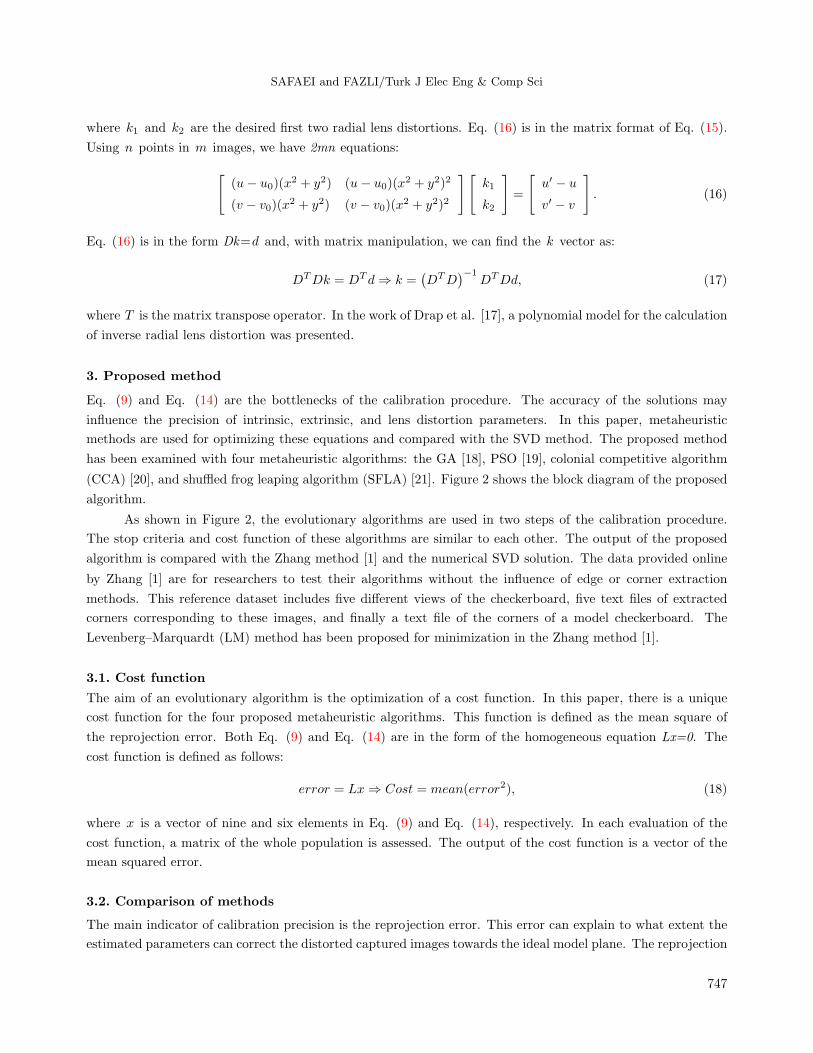
[24]. As shown in Figure 9, the RGB camera has a higher resolution with a wider FOV than the IR camera.

The IR image does not completely overlap with the RGB image; in many applications, the RGB image should

be cropped.

1000

1000 1200 18001400 1600

800

800

600

600

400

200

200 200 600100

50

-50

100

150

200

250

300

350

400

450

400300400

0

0

0 0

Figure 9. Radial lens distortion of Kinect V2: (left) color camera, (right) IR camera.

5.3. Undistortion

From the values of the lens distortion parameters, it is possible to undistort the captured images as shown

in Figures 10 and 11. These outputs may be compared with Figures 6 and 7, respectively. The minority of

distortion parameters causes small changes in the undistorted images in comparison to original ones.

6. Conclusion

This paper proposes four metaheuristic algorithms with one numerical method in the camera calibration process.

Metaheuristic algorithms are used in two stages of the proposed method, and the accuracy and convergence

have improved significantly. We used the GA, PSO, CCA, and SFLA methods in the homography matrix and

752


Figure 10. Undistorted Kinect V1: (top) color images, (bottom) IR images.

Figure 11. Undistorted Kinect V2: (top) color images, (bottom) IR images.

in the intrinsic and extrinsic parameter estimation. In the simulation results, this paper demonstrates that this

method can reduce the total reprojection error criteria in a better way than conventional numerical methods.

The experimental results are noted for both versions of Kinect sensors and the outputs are compared with other

methods in previous studies. This method is practical, especially in applications where matrix manipulation is

time- and power-consuming.

References

[1] Zhang Z. A flexible new technique for camera calibration. IEEE T Pattern Anal 2000; 22: 1330-1334.

[2] Kanatani K. Statistical Optimization for Geometric Computation: Theory and Practice. 1st ed. Amsterdam, the

Netherlands: Elsevier, 1996.

[3] Kanatani K, Takeda S. 3-D motion analysis of a planar surface by renormalization. IEICE T Inf Syst 1995; E78-D:

1074-1079.

[4] Kanatani K. Optimal homography computation with a reliability measure. In: IAPR 1998 Workshop on Machine

Vision Applications; 17–19 November 1998; Chiba, Japan. pp. 426-429.

[5] Hartley R, Zisserman A. Multiple View Geometry in Computer Vision. 2nd ed. New York, NY, USA: Cambridge

University Press, 2004.

[6] Harker MJ, O’Leary PL. Computation of homographies. In: British Machine Vision Conference; 5–8 September

2005; Oxford, UK. pp. 30.1-30.10.

[7] Herrera CD, Kannala J, Heikkila J. Joint depth and color camera calibration with distortion correction. IEEE T

Pattern Anal 2012; 34: 2058-2064.

[8] Raposo C, Barreto JP, Nunes U. Fast and accurate calibration of a Kinect sensor. In: IEEE 2013 International

Conference on 3D Vision; 29 June–1 July 2013; Seattle, WA, USA. New York, NY, USA: IEEE. pp. 342-349.

[9] Ji Q, Zhang Y. Camera calibration with genetic algorithms. IEEE T Syst Man Cy A 2001; 31: 120-130.

753


[10] Hati S, Sengupta S. Robust camera parameter estimation using genetic algorithm. Pattern Recogn Lett 2001; 22:

289-298.

[11] Song X, Yang B, Feng Z, Xu T, Zhu D, Jiang Y, Camera calibration based on particle swarm optimization. In:

IEEE 2009 2nd International Congress on Image and Signal Processing; 17–19 October 2009; Tianjin, China. New

York, NY, USA: IEEE. pp. 1-5.

[12] Merras M, Akkad NE, Saaidi A, Nazih AG, Satori K. Camera self calibration with varying parameters by an

unknown three dimensional scene using the improved genetic algorithm. 3D Research 2015; 6: 1-14.

[13] Tsai RY. An efficient and accurate camera calibration technique for 3D machine vision. In: IEEE 1986 Computer

Vision and Pattern Recognition Conference; 22–26 June 1986; Miami, FL, USA. New York, NY, USA: IEEE. pp.

364-374.

[14] Yılmaz O, Karakus F. Stereo and Kinect Fusion for continuous 3D reconstruction and visual odometry. Turk J Elec

Eng & Comp Sci 2016 24: 2756-2770.

[15] Han J, Shao L, Xu D, Shotton J. Enhanced computer vision with Microsoft kinect sensor: a review. IEEE T Cybern

2013; 43: 1318-1334.

[16] Zhang Z. Camera calibration. In: Medioni G, Kang SB, editors. Emerging Topics in Computer Vision. Upper Saddle

River, NJ, USA: Prentice Hall, 2005. pp. 5-44.

[17] Drap P, Lefevre J. An exact formula for calculating inverse radial lens distortions. Sensors 2016; 16: 1-18.

[18] Holland JH. Adaptation in Natural and Artificial Systems. 1st ed. Ann Arbor, MI, USA: University of Michigan

Press, 1975.

[19] Kennedy J, Eberhart R. Particle swarm optimization. In: IEEE 1995 Neural Networks International Conference;

27 November–1 December 1995; Perth, Australia. New York, NY, USA: IEEE. pp. 1942-1948.

[20] Atashpaz-Gargari E, Lucas C. Imperialist competitive algorithm: An algorithm for optimization inspired by

imperialistic competition. In: IEEE 2007 Evolutionary Computation Congress; 25–28 September 2007; Singapore.

New York, NY, USA: IEEE. pp. 4661-4667.

[21] Eusuff M, Lansey K, Pasha F. Shuffled frog-leaping algorithm: a memetic meta-heuristic for discrete optimization.

Eng Optimiz 2006; 38: 129-154.

[22] Karan B. Accuracy improvements of consumer-grade 3D sensors for robotic applications. In: IEEE 2013 Intelligent

Systems and Informatics Symposium; 26–28 September 2013; Subotica, Serbia. New York, NY, USA: IEEE. pp.

141-146.

[23] Pagliari D, Pinto L. Calibration of Kinect for Xbox One and comparison between the two generations of Microsoft

sensors. Sensors 2015; 15: 27569-27589.

[24] Butkiewicz T. Low-cost coastal mapping using Kinect v2 Time-of-flight cameras. In: IEEE 2014 Oceans Conference;

14–19 September 2014; St. John’s, Canada. New York, NY, USA: IEEE. pp. 1-9.

754

Documents

A novel solution in the simultaneous deep optimization …journals.tubitak.gov.tr/elektrik/issues/elk-18-26-2/elk-26-2-10... · algorithm, with a numerical ... {Marquardt algorithm