Embed Size (px)
Citation preview

1
A Novel Heat Exchanger Design Method Using a Delayed Rejection Adaptive
Metropolis Hasting Algorithm
Ahad Mohammadi1, Javier Bonilla2,3,*, Reza Zarghami1,*,Shahab Golshan1
1: Process Design and Simulation Research Centre, School of Chemical Engineering, College of
Engineering, University of Tehran, P.O. Box 11155/4563, Tehran, Iran
2: CIEMAT-PSA, Centro de Investigaciones Energéticas, Medioambientales y Tecnológicas,
Plataforma Solar de Almería, Spain
3: CIESOL, Solar Energy Research Center, Joint Institute University of Almería - CIEMAT,
Almería, Spain
Abstract
In this study, a shell-and-tube heat exchanger (STHX) design based on seven continuous
independent design variables is proposed. Delayed Rejection Adaptive Metropolis hasting
(DRAM) was utilized as a powerful tool in the Markov chain Monte Carlo (MCMC) sampling
method. This Reverse Sampling (RS) method was used to find the probability distribution of
design variables of the shell and tube heat exchanger. Thanks to this probability distribution, an
uncertainty analysis was also performed to find the quality of these variables. In addition, a
decision-making strategy based on confidence intervals of design variables and on the Total
Annual Cost (TAC) provides the final selection of design variables. Results indicated high
* Corresponding authors:
Tel.: +34 950 387 800; fax: +34 950 365 015; E-mail: [email protected] (J. Bonilla).
Tel.: +98 21 6696 7797; fax: +98 21 6646 1024; E-mail: [email protected] (R. Zarghami).

2
accuracies for the estimation of design variables which leads to marginally improved
performance compared to commonly used optimization methods. In order to verify the capability
of the proposed method, a case of study is also presented, it shows that a significant cost
reduction is feasible with respect to multi-objective and single-objective optimization methods.
Furthermore, the selected variables have good quality (in terms of probability distribution) and a
lower TAC was also achieved. Results show that the costs of the proposed design are lower than
those obtained from optimization method reported in previous studies. The algorithm was also
used to determine the impact of using probability values for the design variables rather than
single values to obtain the best heat transfer area and pumping power. In particular, a reduction
of the TAC up to 3.5% was achieved in the case considered.
Keywords: Shell and Tube Heat Exchanger, Markov chain Monte Carlo, Reverse Sampling,
Delayed Rejection Adaptive Metropolis Hasting
1. Introduction
Heat exchangers are significant and integral components in chemical industries, they are used for
a variety of applications including energy saving, exchange, and recovery[1]. Shell and tube heat
exchangers (STHXs) are commonly used in chemical processes, power plants, and air
conditioning, thanks to the numerous advantages they offer over other types of heat
exchangers[2]. An efficient heat exchanger contributes to lower the consumption of the energy
resources and materials, providing both economic and environmental benefits. The most
conventional method used for heat exchanger design is the iterative process based on trial and

3
error. This approach highly relies on the designer’s experience and generally leads to over-
designed parameters [3]. Several shell and tube heat exchanger design methods are discussed in
handbooks, which are generally based on trial-and-error approaches [2, 4-6].
Optimization of heat exchangers has been studied by different researchers where optimization
algorithms have been used to find the optimum design parameters (the optimization algorithm is
selected based on the type of variables: discrete or continuous) [3]. Wildi-Tremblay and Gosselin
[7] presented a procedure for minimizing the cost of a shell-and-tube heat exchanger based on
genetic algorithms. In their work, evaluations of the performances of heat exchangers were based
on an adapted version of the Bell–Delaware method [8]. Their results showed that the procedure
can properly and rapidly identify the optimal design for a specified heat transfer process.
Selbaset et al. [9] proposed the application of a genetic algorithm (GA) for optimal design of
shell-and-tube heat exchangers. In their research, approximate design methods were investigated
and a generalized procedure was developed to run the GA algorithm in order to find the global
minimum heat exchanger area. The authors found out that combinatorial algorithms, such as
genetic algorithms, provide significant improvement compared to traditional design strategies for
finding the optimum design. Hadidi et al.[10] developed a new shell and tube heat exchanger
optimization design approach based on a biogeography-based optimization (BBO) algorithm.
They applied the BBO technique to minimize the total cost of the equipment including capital
investment and the sum of discounted annual energy expenditures related to pumping in the heat
exchanger. Their results indicated that the BBO algorithm could be successfully applied for the
design of shell and tube heat exchangers.
Ponce-Ortega et al. [11] used a genetic algorithm for the optimal design of shell-and-tube heat
exchangers. They used Bell–Delaware correlations [8] to properly calculate heat transfer

4
coefficients and pressure drops in the shell-side, considering the minimization of the Total
Annual Cost (TAC) as an objective function.Fesanghary et al.[12] used a harmony search
algorithm for minimizing the total cost of shell and tube heat exchangers. They applied global
sensitivity analysis to identify the geometrical parameters that have the largest impact on the
total cost of STHXs. Their results revealed that the proposed algorithm could converge to
optimal solutions with higher accuracy than genetic algorithm.
Caputo et al. [13] carried out economic optimizations of heat exchanger designs using GAs.
They proposed a method for the design of shell and tube heat exchangers based on a genetic
algorithm. They achieved a reduction of capital investment up to 7.4% and savings in operating
costs up to 93%, with an overall reduction of total cost up to 52%.
Hadidi [14] investigated a robust approach for optimal design of plate fin heat exchangers using
a biogeography based optimization algorithm. The author’s parametric analysis was carried out
to evaluate the sensitivity of the proposed method with respect to the cost and structural
parameters.Özçelik [15] developed and applied a genetic algorithm to estimate the optimal
values of discrete and continuous variables in Mixed Integer Non Linear Programming (MINLP)
test problems. Their results over the test problems showed that the programmed algorithm could
estimate acceptable values of continuous variables and optimal values of integer variables.
Finally, such algorithm was extended for parametric studies and for finding optimum
configuration of heat exchangers.
Hilbert et al. [16] developed a multi-objective optimization approach based on a genetic
algorithm to find the most favourable geometry to simultaneously maximize the blade shape of
the heat exchanger while at the same time minimizing the pressure loss. They considered the
coupling of flow / heat transfer processes.Turgut [17] proposed a hybrid approach, entitled

5
Hybrid Chaotic Quantum behaved Particle Swarm Optimization (HCQPSO), for thermal design
of plate fin heat exchangers. He tested the algorithm efficiency with different benchmark
problems and compared them with those of other metaheuristic algorithms. His results revealed
that HCQPSO finds far better solutions minimizing the objective functions compared to designs
and methods reported in the literature.
Ayala et al.[18] presented a Multi-Objective Free Search approach combined with Differential
Evolution (MOFSDE) for heat exchanger optimization. Their results indicated that MOFSDE
shows better performance than the Non-dominated Sorting Genetic AlgorithmII (NSGA-II).
Huang et al. [19] proposed a multi-objective design optimization strategy based on genetic
algorithms for U-tube vertical heat exchangers. Their results showed that the proposed strategy
can decrease the total cost of the system (i.e. the upfront cost and 20 years’ of operation cost) by
9.5% as compared to the original design. Compared to a single-objective design optimization
strategy, 6.2% more energy could be saved by using their multi-objective design optimization
strategy.Habimana [20] developed a model using NSGA-II for the design optimization together
with the MCMC method for uncertainty analysis. His model minimized the area of the system
and the momentary heat recovery output.
Results of optimization algorithms and traditional design methods are expressed as single values
for design variables which do not give any information about the quality and uncertainty of the
parameters.
In the present work, the values of the target variables (heat exchanger area and pump power)
were estimated by sampling design variables using the DRAM method to obtain the heat
exchanger design variables distributions. The design variables are: baffle spacing, baffle cut,
tube-to-baffle diametrical clearance, shell-to-baffle diametrical clearance, tube length, tube outer

6
diameter, and tube wall thickness, which were estimated considering their uncertainty bands
rather than a fixed value. With this algorithm, the presented uncertainty analysis could be
accomplished more thoroughly and uncertainty bands could be studied more accurate than in
comparison with other methods. In addition, a conventional shell and tube heat exchanger, as a
case of study, was used for the validation of the proposed technique and results were compared
to multi-objective and single-objective optimization methods. Finally, a cost function is defined
and a decision making process was established for the selection of the design variables based on
their estimated distributions and TAC.
2. Sampling Methods
Sampling can be used to predict the behaviour of a particular model under a set of defined
circumstances in order to find appropriate values for the model parameters by fitting model
results to experimental data [21]. One of the most significant benefits of using sampling
algorithms is the ability of these methods to analyse uncertainties. In sampling methods, the
decision-making process is essential for the selection of the final variables among a set of
samples.
In statistics, Markov Chain Monte Carlo (MCMC) methods are algorithms for sampling:
Adaptive Metropolis (AM) and Delayed Rejection (DR) are two methods for improving the
MCMC performance [22]. The main insight behind AM is its ability to perform on-line tuning of
the proposed distribution based on the past sample path of the chain [23]. The rationale behind
adaptive strategies is to learn from the information obtained during the run of the chain, and
based on this, to efficiently tune the proposals. The acceptance probability of the second stage

7
candidate is computed so that the reversibility of the Markov chain relative to the intuition
distribution is preserved. The basic idea of DR is based upond rejection of a proposed candidate
point, instead of retaining the same position, a second stage move is proposed [24].The details of
the DRAM method are presented in appendix 2.
In this paper, DRAM was used to obtain the probability distribution of design variables of the
shell and tube heat exchanger. An advantage of this method is its ability to express the design
variables in the form of probabilistic distributions with a confidence interval. Confidence
intervals provide an essential understanding of how much faith we can have in our sampling and
provide the most likely range for the unknown population of all variables.Unlike optimization
algorithms, sampling methods can represent the uncertainty of variables. Uncertainty analysis is
useful in real processes where deviations from set points affect the performance of the system.
To perform a quantitative uncertainty analysis, probability distributions should be assigned to
each design variable.
2.1. Design Variables
Seven continuous decision variables are considered in the sampling process in order to obtain the
values of the area and pumping power based on the design algorithm presented in Appendix 1.
The DRAM method changes the values of these seven variables. The algorithm in Appendix 1
takes those values and calculates the area and pumping power. This sampling procedure run until
stable probability distributions of the design variables, heat exchanger area and pumping power,
are obtained. The probability distributions of the design variables are assumed to be Gaussian.
The specifications of the design variables are as follows [3]:

8
• The baffle spacing at the centre, inlet, and outlet (Lbc = Lbo= Lbi) varies between the
minimum baffle spacing of 0.0508 m and the maximum supported tube span of 0.2540 m
(referring to X1 in fig.1) [25].
• The baffle cut (Bc) can vary from 15 % to 45 %( referring to X2 in fig.1).
• Tube-to-baffle diameter clearance (δtb) can take values between 0.01do m and 0.1do m
(referring to X3 in fig.1).
• Shell-to-baffle diametrical clearance (δsb) is between 0.0032 m and 0.011 m [26]
(referring to X4 in fig.1).
• The tube length (L) : 2.438 and 11.58 m [26] (referring to X5 in fig.1).
• The tube outer diameter (do): [0.01588 to 0.0508] m (referring to X6 in fig.1).
• The tube wall thickness: [1.651, 4.572] mm (referring to X7 in fig.1).
A schematic sampling network is illustrated in Fig. 1, which corresponds with the third step of
the process represented in Fig. 2.

9
Fig. 1. Schematics of design and target variables.
The top nodes are target variables (area and pumping power) and the bottom nodes are design
variables. In this figure, the target variables dependence on the design variables is shown.
3. Results and Discussion
DRAM was carried out for a case of study selected from the literature [7] to test the
performance of the sampling algorithm for obtaining values for the design variables of a shell-
and-tube heat exchanger. In addition, the results of the proposed method were compared with
previous methods for design optimization [3]. For this case of study, 30,000 samples were
considered.
10
Fig. 2 shows the designing procedure flowchart, which is proposed and used in this research.
Seven steps can be found on the flowchart which are described in the following:
• Step (1): The governing equations on the shell-and-tube heat exchanger, design variables
and target variables are specified.
• Step (2): The initial values of the design variables, used in the DRAM method, are set
according to their ranges.
• Step (3): The DRAM algorithm performs the sampling of the design variables in this
step.
• Step (4): The heat exchanger area and pumping power are calculated for each instance of
the design variables in this step.
• Step (5): The new calculated values are compared with the present values in order to
reach the stable distribution of the design variables.
(The probability distribution of design variables does not change when increasing number
of samples. As the number of samples increases, the probability distribution of the design
variables converges to a unique distribution. It became clear that when the number of
samples exceeds 30,000, a stable distribution is obtained.)
• Step (6): Samples are obtained for each design variable. (When the sampling is
completed, for each one of the design variables, a Gaussian probability distribution with
given variance and mean values is obtained.)
• Step (7): The selection of a set of the design variables, based on the decision making
strategy (see Fig. 4), is performed in this step.

11
Fig. 2. Flowchart of the design procedure

12
For the initial guess, the sampling begins with the arithmetic mean value of the design variables
in their ranges, and a variance value of ±2σ of the limit for each variable. It should be considered
that according to the DRAM method; every random choice for the mean value in this limit makes
the sampling algorithm converge [27]. Similarly, for the specific variance, 99.8 % of data are
located inside -3σ to +3σ (σ denotes variance); however in this work initial limits are set to ±2σ
of the limit as stated before, in order to have a higher confidence. The design variables are
improved towards the desired target variable values at each sampling iteration. The sampling
process continues up to the point where all the nodes, including the design variables, reach their
stable distributions.
A confidence interval of 90% was considered for the design variables. Fig. 3 depicts the samples
of the design variables and the resulting overall heat exchanger area for each set of samples. Two
elliptical shapes are shown in this figure; the inner and outer curves illustrate the regions that
contain 50% and 90 % of the samples around their mean values, respectively.
40
90
140
190
240
290
340
29 34 39 44 49 54
Pu
mp
ing p
ow
er (
w)
Area (m2)
50%
90%
0,02
0,06
0,1
0,14
0,18
29 34 39 44 49 54
Baff
le s
pa
cin
g (
m)
Area (m2)
50%
90%

13
Fig. 3. Probability distribution of design variables as a function of the heat exchange surface area
In order to test the modelling results, a case of study considering the cooling of Naphtha using
water in a shell-and-tube heat exchanger is presented. The operational data is used for validation
(see Table 1). The results from the sampling method, in terms of mean and variance of the
0,03
0,13
0,23
0,33
29 34 39 44 49 54
Baff
le c
ut
Area (m2)
50%
90%
-5,E-05
-2,E-19
5,E-05
1,E-04
2,E-04
2,E-04
29 34 39 44 49 54
Tu
be b
aff
le c
learan
ce (
m)
Area (m2)
50%
90%
0,0031
0,0032
0,0033
0,0034
0,0035
0,0036
0,0037
29 34 39 44 49 54
Sh
ell
baff
le c
learan
ce (
m)
Area (m2)
50%
90%2,5
3
3,5
4
4,5
5
5,5
6
29 34 39 44 49 54
Tu
be l
ength
(m
)
Area (m2)
50%
90%
0,01921
0,01926
0,01931
0,01936
0,01941
0,01946
29 34 39 44 49 54
Tu
be o
ute
r d
iam
ete
r (
m)
Area (m2)
50%
90%
1,75E-03
1,85E-03
1,95E-03
2,05E-03
2,15E-03
2,25E-03
29 34 39 44 49 54
Tu
be w
all
th
ick
ness
(m
)
Area (m2)
50%
90%

14
Gaussian distributions of the design variables, have been compared to results in the literature [7]
in Table 2. It should be noted that most of the approaches reported in literature for heat
exchanger optimization are based on single values for the design variables, but in this study, we
present probability distributions for all the design variables.
Tube-side Shell-side
Fluid Cooling water Naphtha
Flow rate (kg/s) 30 2.7
Inlet temperature (oC) 33 114
Outlet temperature (oC) 37.21 40
Density (kg/m3) 1000 656
Heat capacity (J/(kg K)) 4186.8 2646.06
Viscosity (N s/m2) 0.00071 3.70 *10-4
Thermal conductivity (W/m K) 0.63 0.11
Design pressure (Pa) 1278142 738767
Fouling resistance (m2 K/W) 0.0004 0.0002
Material of construction Stainless steel Carbon steel
Wall thermal conductivity (W/(m K)) 16 55
Table 1. Design data used for validation [7]
Parameter
DRAM Single-objective
optimization
Multi-objective
optimization mean Variance
Baffle spacing(m) 0.0956 9.2e-03 0.06 0.079

15
Baffle cut (%) 23.10 3.1 25 16.515
Tube-to-baffle diameter
clearance(mm)
0.24864 9.0e-2 0.381 0.204
Shell-to-baffle diametrical
clearance(mm)
3.4 7.0e-01 3 3.279
The tube length(m) 4.292 0.881 10.7 3.426
The tube outer
diameter(mm)
23.4 3.813 38.1 19.578
The tube wall thickness(mm) 2.05 0.634 3.405 1.652
Table 2. DRAM calculated variables compared to multi-objective and single-objective
optimizations
The optimum values from [3] are used as target function values for the sampling algorithm. The
sampling method performed 30,000 iterations. The results show good performance with respect
to the design variables estimation compared to the optimization methods. As estimated,
incrementing the number of iterations leads to more accurate results. By increasing the number
of samples, it was found that the result values almost did not change and it can be stated that
convergence was achieved, which indicates a stable distribution of the design variables.
Fig. 4 presents the mean values and uncertainty bands of the independent variables used in the
DRAM sampling compared to the results from multi-objective and single-objective
optimizations. As stated previously, the results of optimization algorithms are described as fixed
values without any estimation about the possible deviations from these points. As illustrated in
Fig.4, the uncertainty band of the tube to baffle diameter clearance has the widest band among all
variables, while the tube outer diameter, tube wall thickness, tube length and baffle spacing
variables have narrow distributions around their mean values. In other words, these variables are

16
less likely to deviate from their mean. Additionally, this probability distribution can help in the
decision-making process. If, under any circumstance, the manufacturer cannot use the proposed
design values, then other values for the design variables can be selected.
0,0
0,2
0,4
0,6
0,8
1,0
0,1 0,2 0,3 0,4 0,5
Prob
ab
ilit
y
Tube to baffle diameter clearance (mm)
Multi Objective
Single Objective0,0
0,2
0,4
0,6
0,8
1,0
1 2 3 4
Prob
ab
ilit
y
Tube wall thickness (mm)
Multi Objective
Single Objective
0,0
0,2
0,4
0,6
0,8
1,0
17 27 37
Prob
ab
ilit
y
The tube outer diameter (mm)
Multi Objective
Single Objective0,0
0,2
0,4
0,6
0,8
1,0
2,9 7,9
Prob
ab
ilit
y
Tube length (m)
Multi Objective
Single Objective
0,0
0,2
0,4
0,6
0,8
1,0
2,7 3,2 3,7
Prob
ab
ilit
y
Shell to baffle diameter clearance …
Multi Objective
Single Objective0,0
0,2
0,4
0,6
0,8
1,0
15 20 25 30 35
Prob
ab
ilit
y
Baffle cut (%)
Multi Objective
Single Objective

17
Fig. 4.Probability distribution of design variables compared to multi-objective and single-objective
optimizations
A cost analysis method was used for the selection of the final design variables in the decision-
making process. The global annual cost includes the operating cost and the initial cost expressed
in terms of annuities, it was used in the decision making process for selecting the values of the
design variables.
Fig. 5 sketches the decision making process, which involves the following steps:
• Goal: To get the best values for the design variables.
• Step (1): Select TAC as the decision variable.
• Step (2): Obtain sets of design variables with the DRAM method and the multi-objective
genetic algorithm.
• Step (3): Calculate the TAC for all sets of design variables that are obtained from both
methods.
• Step (4) Choose the set of design variables which has the lowest TAC.
0,0
0,2
0,4
0,6
0,8
1,0
0,05 0,09 0,13 0,17P
rob
ab
ilit
yBaffle spacing (m)
Multi Objective
Single Objective

18
Fig 5. Flowchart of the decision making process
Fig. 6 shows the TAC associated with each sample together with the obtained from the multi-
objective optimization. In Fig.6, a lower TAC means better design variables. The sets of design
variables predicted by the DRAM method have lower TAC compared to the multi-objective
optimization in most of the cases.

19
Fig. 6. Cost analysis for decision-making of multi-objective optimization [3] vs. DRAM
sampling
From the results presented in Table 3, it can be inferred that the DRAM algorithm is suitable for
the design of shell and tube heat exchangers. In the studied case, the TAC was drastically
reduced and a significant percent of TAC reduction was achieved compared to the traditional
design method. A TAC percentage decrease of 3.52% was obtained, which confirms the
effectiveness of the proposed approach. As a final remark, it should be noted that the sampling
method design generally leads to a heat exchanger structure markedly different from that
considered as a conventional design.
Parameter
DRAM Single-objective
Optimization
Multi-objective
Optimization Mean variance
Ao (m2) 37.16 5.32 37.14 37.14
∆PS, shell-side (Pa) 21632 1543.3 22600 20620
1000
3000
5000
7000
9000
15 25 35 45
Cost
($/y
ear)
Area (m2)
GA
MCMC

20
∆Pt tube side (Pa) 8697 1223 8600 8584
Table 3. Comparison between sampling algorithm, multi-objective and single-objective
optimizations using 30,000 samples
4. Conclusions
The DRAM sampling method was used to design a shell-and-tube heat exchanger. Based on the
proposed approach, an algorithm was developed, and a case of study was investigated to
illustrate its effectiveness, efficiency and suitability of the proposed method. Uncertainty
analysis through uncertainty bands measured, and the deviations from mean values, were plotted
for all of the design parameters. A decision-making strategy based on a confidence interval and
TAC was used for final design variable selection. Results demonstrate accurate design variables
values when compared with those obtained from optimization methods. The DRAM method
presents lower TAC by choosing more appropriate design variable values.
Results indicate that DRAM can provide an estimation of the confidence interval for design
variables, comparing the interval range to previously published values.. This method shows that
design variables, in addition to the most likely value, have a confidence interval for evaluating
their quality. The main advantages of the sampling method are that the designer can choose one
particular solution from distribution solutions based on the proposed desicion making process, as
well as estimating the cost of a particular design. With respect to the test case, a reduction of
TCA of 3.52% was obtained, which shows the potential of the proposed method for improving
the design of more cost-effective heat exchangers.

21
Acknowledgements
The results presented in this paper have been obtained within collaboration with IPS Company.
The financial support is gratefully acknowledged.
Appendix 1
Fig. 7 shows a schematic view of a shell-and-tube heat exchanger. The overall heat transfer
coefficient based on tube outer diameter U0 is given by (1) [2].
Fig.7. Schematics of a shell-and-tube heat exchanger
0
0
1
ln( / )1 1
2o o i o o
s t
W i i i
Ud d d d d
R Rh k d h d
=
+ + + +
, (1)

22
where ho and hi are the shell-side and tube-side heat transfer coefficients, do and di are the outer
and inner tube diameters, Rs and Rt are fouling resistances on the shell and tube sides, and kw is
the tube wall thermal conductivity. The heat exchange area is calculated by (2) [2]:
0
0 lm
QA
U T F=
, (2)
Before calculating the area, the value of U0 should be estimated. After that, the system of
equations is solved again using the new calculated area and a corrected area is calculated to be
used in the next step. This algorithm continues to a step where the area reaches convergence.
The fundamental equations for heat transfer across a surface is given by [2]:
, , , , , ,( ) ( )h p h h i h o c p c c o c iQ m c T T m c T T= − = − , (3)
The log-mean temperature difference (Tlm) is defined as [2]:
, , , ,
, ,
, ,
( ) ( )
ln
h i c o h o c i
lm
h i c o
h o c i
T T T TT
T T
T T
− − − =
− −
, (4)
F is the log-mean temperature difference correction factor for a special layout. It can be shown
that in general it depends on the heat capacity rate ratio (R) and correctness coefficient (S) [2]:

23
2
2
2
1( 1) ln( )
1
2 ( 1 1)( 1) ln
2 ( 1 1)
SR
RSF
S R RR
S R R
−+
−
− + − +−
− + + +
, (5)
, ,
, ,
( )
( )
h i h o
c o c i
T TR
T T
−=
−, (6)
, ,
, ,
c o c i
h i c i
T TS
T T
−=
−, (7)
Tube pitch, centre-to-centre distance between tubes, should not be less than 1/25 times the
outside diameter. On the other hand, very high values result in an increment of the shell
diameter. As a result:
1.25t oP d= , (8)
Having the tube diameter, length and area values; the required number of tubes can be calculated
using (9).
t
o t
AN
d L= , (9)
The outer tube diameter limit is calculated as:

24
1
1
1
nt
otl o
ND d
K
=
, (10)
K1 and n1 values for different tube configurations are given in Table 4 [28].
Number of passes
Triangular pitch Square and rotated square
K1 n1 K1 n1
1 0.319 2.142 0.215 2.207
2 0.249 2.207 0.156 2.291
3 0.175 2.285 0.158 2.263
Table 4. Parameters used for the calculation of the tube bundle diameter [22]
The shell diameter is calculated from:
0.95
otls sb
DD = + , (11)
Where, δsb is the shell-to-baffle clearance.
Shell-side heat transfer
The shell-side heat transfer coefficient hs is determined by Eq. 12 by means of correcting the
ideal heat transfer coefficient hid for various leakage and bypass flow streams in a baffled

25
segment of the shell-and-tube exchanger. The hid is determined for pure cross flow in a
rectangular tube bank assuming that the entire shell-side stream flows across the tube bank at or
near the centreline of the shell. It is computed from the Chilton and Colburn j factor.
Many formulations are recommended for the calculation of these values. The following equation
is suggested by Shah and Sekulic [2]:
s id c s rh h J J J J= , (12)
2
3
,
Prs ps
id
o cr
jm ch
A
−
= , (13)
In the above equation, Ao,cr is the flow area at or near the shell centerline for one cross-flow
section in the shell-and-tube exchanger, j is the colburn factor, cps is the specific heat capacity of
the fluid in the shell side, where the Prandtl number is given by:
Prps s
s
c
k
= , (14)
For the calculation of the j parameter value, a set of correlations are used [2, 7]:
2
1
1.33(Re )
/
a
a
s
T o
j aP d
=
, (15)
4
3
1 0.14(Re )a
s
aa =
+, (16)
The values of a, a1, a2, and a3 are given in Table 5 [28]. Additionally, Res is calculated from the
following equation.

26
Layout
angle
Reynolds
number
a1 a2 a3 a4 b1 b2 b3 b4
45o
105-104 0.370 -0.396 1.930 0.500 0.303 -0.126 6.59 0.520
104-103 0.370 -0.396 - - 0.333 -0.136 - -
101-102 0.730 -0.500 - - 3.500 -0.476 - -
102-101 0.498 -0.656 - - 26.200 -0.913 - -
<10 1.550 -0.667 - - 32.000 -1.000 - -
Table 5. Colburn factor (j) coefficients and ideal friction factor (fid) [28]
,
Re s os
s o cr
m d
A= , (17)
The correction factor for the baffle configuration (Jc) is dependent on the fraction of the total
number of tubes in cross flow between baffle tips [2]:
0.55 0.72c cJ F= + , (18)
where Fc represents the fraction of the total number of tubes in the cross-flow section. The Jc
value is 1.0 for heat exchangers with no tubes. This values increases to 1.15 for small baffle cuts
and decreases to 0.65 for large baffle cuts [2].
The angle in radians between the baffle cut and two radii of a circle through the canters of the
outermost tubes is as follows [2]:

27
1 22cos s c
ctl
ctl
D
D − −
=
, (19)
sin1 2 1 ctl ctl
c wF F
= − = − + , (20)
ctl otl oD D d= − . (21)
The correction factor for baffle leakage effects (Jl)), including both, tube-to-baffle and baffle-to-
shell leakages with heavy weight constructions, is given by (22). It is function of the ratio of the
total leakage area per baffle to the cross-flow area between adjacent baffles, and also of the ratio
of the shell-to-baffle leakage area to tube-to-baffle leakage area. If baffles are too close, Jl will
have a lower value, due to higher flows of leakage streams. A typical value of Jl is in the range
0.7 to 0.8.
2.210.44(1 ) [1 0.44(1 )] lm
s sJ r r e −= − + − − , (22)
,
, ,
o sb
s
o sb o tb
Ar
A A=
+ ,
, ,
,
o sb o tb
lm
o cr
A Ar
A
+= , (23)
The correction factor for bundle and pass partition bypass streams (Jb) varies from 0.9, for a
relatively small clearance between the outermost tubes and the shell for fixed tube sheet
construction, to 0.7, for large clearances in pull-though floating head construction. Its value can
be increased from 0.7 to 0.9 by proper use of the sealing strips in a pull-through bundle.

28
1/3
1
exp[ (1 (2 ) )]b
b ss
JCr N +
=
− −
1/ 2
1/ 2
ss
ss
forN
forN
+
+
, (24)
,
,
o bp
b
o cr
Ar
A= , (25)
,
ssss
r cc
NN
N
+ = , (26)
1.35
1.25C
=
for
for
Re 100
Re 100
s
s
, (27)
The magnitude of the cross-flow area of the flow bypass is given by:
, , ( 0.5 )o bp b c s otl p pA L D D N w= − + , (28)
The number of tube rows Nr,cc, crossed through one cross-flow section between baffle tips may
be obtained from a drawing or directly counting. It may be also estimated from the following
expression:
,
2s cr cc
DN
X
−= , (29)
The cross-flow area at or near the shell centreline for one cross-flow section may be estimated
from:

29
, ,[ ( )]ctlo cr s otl t o b c
t
DA D D X d L
X= − + − , (30)
Js is the correction factor for larger baffle spacing at the inlet and outlet sections compared to the
central baffle spacing. The nozzle locations result in larger end baffle spacing and lower
velocities, and thus lower heat transfer coefficients. Js usually varies from 0.85 to 1.0.
1 11 ( ) ( )
1
n n
b i os
b i o
N L LJ
N L L
+ − + −
+ +
− + +=
− + +, (31)
,
,
b i
i
b c
LL
L
+ =,
,
b o
o
b c
LL
L
+ = , (32)
0.6
1/ 3n
=
for
for min
turbulent
la ar
flow
flow , (33)
In this study, it was assumed that Lb, c = Lb, i = Lb,o, and thus Js = 1. The correction factor for
adverse temperature gradient in laminar flow, Jr, was not taken into consideration in this study
and was set to 1.
Tube-side heat transfer
When designing heat exchangers, pressure drop considerations are commonly important factors
that must be studied in detail. The heat transfer coefficient of the tube side, hi, is given by [2]:

30
0.14
1/3 0.80.023 Pr Ret ti t t
i tw
kh
d
=
, (34)
where the tube-side Reynolds number is:
Re t t it
t
V d
= , (35)
the Prandl number of the liquid in the tube-side is:
Prpt t
t
t
c
= , (36)
The velocity of the fluid in the tubes, Vt, is calculated with the following equation [2]:
2( / 4)
p tt
t i t
N mV
N d = , (37)
Shell-side pressure drop
There are several ways to estimate the pressure drop in the shell side. In this work, the shell-side
pressure drop is calculated using the Bell-Delaware method, given by the next equation [20]:
,
, , ,
,
[( 1) ] 2 1r cw
s b b id b b w id l b id b s
r cc
NP N P N P P
N
= − + + +
, (38)
where, Nr,cw is the number of effective tube rows in cross flow in each window, and ∆Pb,id is the
pressure drop for liquid flowing in an ideal cross flow between two baffles. It is calculated by
(39) [20]:
0.252
,
,
4
2
id s r cc swb id
s s
f G NP
=
, (39)

31
The friction factor fid associated with the ideal cross flow is expressed as [20]:
2
1
1.33Re
/
b
b
id s
T o
f bP d
=
, (40)
4
3
1 0.14(Re )b
s
bb =
+, (41)
2
,
,
, ,
(2 0.6 )
2
r cw s
w id
s o cr o w
N mP
A A
+ = , (42)
The correction factor ζb is calculated as:
( )1/3exp 2.7 [1 (2 ) ]
1
b s
b
r N
++ − −=
for
for
1/ 2
1/ 2
s
s
N
N
++
++
, (43)
The second correction factor ζl is:
exp( 1.33(1 ) )p
l s lmr r = − + , (44)
[ 0.15(1 ) 0.8]sp r= − + + , (45)
1.8 1.8
, ,
, ,
b c b c
s
b o b i
L L
L L
= +
, (46)
32
Tube-side pressure drop
The tube-side pressure drop is calculated from the following expression [20]:
24
2.52
t tt p
i
VfLP N
d
= +
, (47)
where f is the friction factor for turbulent flow and is given by [20]:
0.20.046(Re )tf −=, (48)
The pumping power for the tube and shell sides is calculated similarly on both sides [20]:
,t t s s
s t
t s
P m P mP
= + , (49)
where, η is considered to be 0.85 [3].
Cost analysis
Cost is always one of the most important factors to take into consideration when designing
industrial equipment. Cost can be broken into two principal components, capital cost and

33
operating cost. In addition, maintenance cost incurred during operation is also an important
factor that must be estimated; nevertheless they tend to be commonly independent of the size of
the heat exchanger. The purchase cost is obtained from the following correlation for ambient
operating pressure and carbon steel material [29].
( )2
1 2 3log log logp o oC K K A K A= + + . (50)
K1, K2 and K3 parameters were determined for a shell-and-tube heat exchanger at a particular
point in time. As a result, the purchase cost corrected, for the effect of changing economic
conditions and inflation, can be calculated with the following correlation.
22 1
1
( )I
C CI
= , (51)
where C is the purchase equipment cost, I is the cost index, subscript 1 indicates the base time
when the cost was determined and subscript 2 the time when the cost is estimated.
The bare module cost CBM of the heat exchanger, which includes the direct and indirect costs for
non-base conditions such as nonambient pressure and materials of construction different from
carbon steel, is given by the following correlation:
( )1 2
o
BM P PM P M PC C F C B B F F= = + , (52)
The pressure factor FP is given by:
34
( )2
1 2 3log log logPF C C P C P= + + , (53)
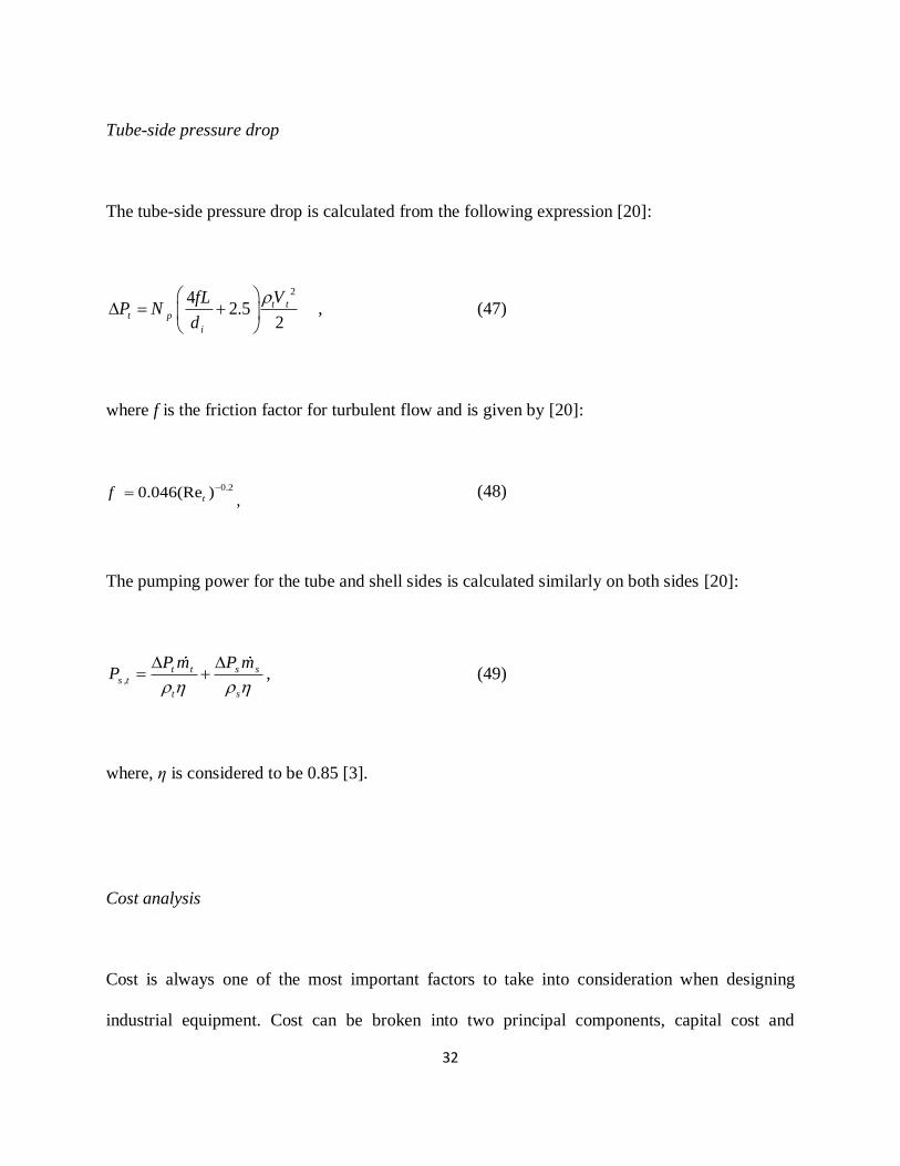
P is measured in bar gauge, the material factor FM, as well as the C1, C2, and C3 coefficients are
listed in Table 6 [29].
Correlation factor Value
K1 3.2138
K2 0.2688
K3 0.07961
C1 0
C2 0
C3 0
FM(shell-CS Tube-Cu) 1.25
FM (shell-CS Tube-SS) 1.7
B1 1.8
B2 1.5
Table 6. Capital cost factors [29]
Pumps must provide work to overcome the pressure drop on the tube side, as well as on the shell
side. The annual operating cost, calculated from the total pumping power (Ps,t) on the tube and
shell sides, is given by [29]:
,8232 s tOC P ec= , (54)

35
where ec is the electricity cost. In the previous equation, ec is assumed to be $0.1 kW-1h-1 [29].
The factor 8232 accounts for the number of hours of operation, assuming that the heat exchanger
is operating 49 weeks during the year.
The TAC of the heat exchanger is expressed in terms of equal annuities of the bare module cost
and the annual operating cost:
( 1)
( 1) 1
n
BM n
i iTC C OC
i
+= +
+ −, (55)
where i is the fractional interest rate per year (i = 0.05) and n is the expected lifespan of the heat
exchanger, which was taken to be 20 years, in order to compare the results obtained in this work
with results from the previously published design in Wildi-Tremblay and Gosselin [7].
Apendix 2
A Markov chain is a stochastic process that transitions from one state to another using a simple
sequential procedure. A Markov chain starts at some state x (1) and use a transition
function 𝑝(𝑥(𝑡)|𝑥(𝑡 − 1)) to determine the next state, x (2) conditionally dependent on the
previous state, the process must keep iterating to create a sequence of X. In this iterative
procedure, the next state of the chain at t+1 is based only on the previous state at t. This is an

36
important property when using Markov chains for MCMC because previous states of the chain
do not affect the state of the chain after one step.
Markov chains converge to a stationary distribution regardless of the starting point. When this
property is applied to MCMC, it allows drawing samples from a distribution using a sequential
procedure where the starting state of the sequence does not affect the final estimation process.
Adaptive metropolis-hastings methods
The basic idea is to create a Gaussian proposal distribution with a covariance matrix which is
calibrated using the sample path of the MCMC chain. The Gaussian proposal is centered at the
current position of the Markov chain, Xn, and its covariance is given by: 𝑛 =
𝑠𝑑𝐶𝑜𝑣(𝑋0, . . . , 𝑋𝑛−1) + 𝑠𝑑𝜀𝐼𝑑, where 𝑠𝑑 is a parameter that depends only on the dimension d of
the state space where π is defined. ε >0 is a constant that we may choose very small. Id denotes
the d-dimensional identity matrix [30]. In order to start the adaptation procedure, an arbitrary
strictly positive definite initial covariance, C0, is chosen according to a priori knowledge. A time
index, n0> 0, defines the length of the initial non-adaptation period.
0
0 1( ,... )n
d n d d
CC
s Cov X X s I−
+
0
0
n n
n n
, (56)
The empirical covariance matrix is determined by the points 𝑋0, . . . , 𝑋𝑘 ∈ 𝑅𝑑 ∶
0 1
0
1( ,... ) ( 1)
kT T
n i i k k
i
Cov X X X X k X Xk
−
=
= − +
, (57)

37
where 1
1
1
k
k iiX X
k ==
+ and the elements X I ∈Rd are considered as column vectors.
Substituting (56) in (57), it is obtained that, the covariance Cn satisfies the recursive formula
when n > n0:
( )1 1 1
1( 1)T T T
n n n n n n n n d
n sdC C nX X n X X X X I
n n+ − −
−= + − + + +
,(58)
which permits the calculation of the covariance matrix without excessive computational cost,
since the mean, Xn, also satisfies a recursive formula.
Delayed rejection
Delaying Rejection (DR) is a strategy that improves the Metropolis-Hasting (MH) algorithm.
Assuming that the position of the chain at time t is Xt=x. A candidate y1 is generated from
q1(x,dy) and accepted with the following probability [27].
1 1 1 11
1 1 1
( ) ( , )( , ) 1 1
( ) ( , )
y q y x Nx y
x q x y D
= =
, (59)
Upon rejection, instead of retaining the same position, Xn+1 = x, as we would do in a standard
MH, a second stage move, Y2, is proposed. The second stage proposal depends not only on the

38
current position of the chain but also on what we have just proposed and rejected: 𝑞2(𝑥, 𝑦1, 𝑦2),
the second stage proposal is then accepted with the following probability [27].
2 1 2 1 2 2 1 1 2 1
2 1 2
1 1 2 1 2 1 1
2
2
( ) ( , ) ( , , ) 1 ( , )( , , ) 1
( ) ( , ) ( , , ) 1 ( , )
1
y q y y q y y x y yx y y
x q x y q x y y x y
N
D
−=
−
=
, (60)
This process of DR can be iterated. If qi denotes the proposal at the i-th stage, the acceptance
probability at that stage is as follows [31]:
1( , ,..., ) 1 ii i
i
Nx y y
D =
, (61)
If the 𝑖𝑡ℎ stage is reached, it means that 𝑁𝑗 < 𝐷𝑗 for𝑗 = 1, . . . , 𝑖 − 1, therefore
𝛼𝑗 (𝑥, 𝑦1, . . . , 𝑦𝑗 ) is simply 𝑁𝑗/𝐷𝑗 , 𝑗 = 1, . . . , 𝑖 − 1 and a recursive formula is obtained.
1 1( ,..., )( )i i i i iD q x y D N− −= −, (62)
which leads to,
1 1 2 2
2 1 2 1 1 1 2 3 1
( ,..., )[ ( ,..., )[ ( ,..., )...
[ ( , , )[ ( , ) ( ) ] ] ]... ]
i i i i i i i
i
D q x y q x y q x y
q x y y q x y x N N N N
− − − −
−
=
− − −, (63)
Since all acceptance probabilities are computed in such a way that reversibility with respect to π
is preserved separately at each stage, the process of DR can be interrupted at any stage, therefore

39
it can be decided in advancethe number of tries before moving away from the current position.
Alternatively, upon each rejection, it can be tossed a p-coin (i.e., a coin with head probability
equal to p), and if the outcome is head, it is moved to a higher stage proposal, otherwise it stays
put.
Nomenclature
Variance Σ
Heat transfer surface area (m2) Ao
Flow area at or near the shell centreline for one cross-flow
section (m2)
Ao,cr
Shell-to-baffle leakage flow area (m2) Ao,sb
Tube-to-shell leakage flow area (m2) Ao,tb
Baffle cut Bc
Specific heat capacity (J kg-1 K) cp
Inside tube diameter (m) di
Outside tube diameter (m) do
Tube bundle outer diameter (m) Dotl
Shell diameter (m) Ds

40
Correction factor for number of tube passes, friction factor F
Fluid mass velocity (kg m2 s-1) G
Heat transfer coefficient (W m-2 K-1) h
Correction factor for shell-side heat transfer J
Thermal conductivity (W m-1 K-1) k
Baffle spacing at center, inlet, and outlet (m) Lbc = Lbo= Lbi
Tube length (m) L
Mass flow rate (kg s-1) m
Number of baffles Nb
Number of tube passes Np
Number of sealing strip pairs Nss
Total number of tubes Nt
Prandtl number Pr
Tube pitch (m) Pt
Pumping power on tube and shell sides (W) Ps,t
Heat duty (W) Q
Fouling resistance (m2 k W-1) R

41
Reynolds number Re
Tube thickness (m), Temperature (oC) T
Overall heat transfer coefficient (W m-2 K-1) Uo
Flow velocity (m s-1)
Greek symbols
Shell-side pressure drop correction factor
Viscosity (Pa s)
Density (kg m-3)
Tube-to-baffle diameter clearance δtb
Shell-to-baffle diametrical clearance δsb
Efficiency
Angle in radians ctl
Pressure drop P
Log-Mean temperature difference
lmT
Subscripts and superscripts

42
Cold fluid, center of the heat exchanger C
Hot fluid H
Tube inlet I
Ideal Id
Tube outlet O
Shell side S
Tube side T
Tube wall W
References
[1] S. Kakac, H. Liu, A. Pramuanjaroenkij, Heat exchangers: selection, rating, and thermal
design, CRC press, 2012.
[2] R.K. Shah, D.P. Sekulic, Fundamentals of heat exchanger design, John Wiley & Sons, 2003.
[3] S. Fettaka, J. Thibault, Y. Gupta, Design of shell-and-tube heat exchangers using
multiobjective optimization, International Journal of Heat and Mass Transfer, 60 (2013) 343-
354.
[4] E.U. Schlunder, Heat exchanger design handbook, (1983).
[5] S.T.M. Than, K.A. Lin, M.S. Mon, Heat exchanger design, World Academy of Science,
Engineering and Technology, 46 (2008) 604-611.

43
[6] E. Saunders, Heat exchangers, (1988).
[7] P. Wildi‐Tremblay, L. Gosselin, Minimizing shell‐and‐tube heat exchanger cost with genetic
algorithms and considering maintenance, International Journal of Energy Research, 31 (2007)
867-885.
[8] K.J. Bell, Final report of the cooperative research program on shell and tube heat exchangers,
University of Delaware, Engineering Experimental Station, 1963.
[9] R. Selbaş, Ö. Kızılkan, M. Reppich, A new design approach for shell-and-tube heat
exchangers using genetic algorithms from economic point of view, Chemical Engineering and
Processing: Process Intensification, 45 (2006) 268-275.
[10] A. Hadidi, A. Nazari, Design and economic optimization of shell-and-tube heat exchangers
using biogeography-based (BBO) algorithm, Applied Thermal Engineering, 51 (2013) 1263-
1272.
[11] J.M. Ponce-Ortega, M. Serna-González, A. Jiménez-Gutiérrez, Use of genetic algorithms
for the optimal design of shell-and-tube heat exchangers, Applied Thermal Engineering, 29
(2009) 203-209.
[12] M. Fesanghary, E. Damangir, I. Soleimani, Design optimization of shell and tube heat
exchangers using global sensitivity analysis and harmony search algorithm, Applied Thermal
Engineering, 29 (2009) 1026-1031.
[13] A.C. Caputo, P.M. Pelagagge, P. Salini, Heat exchanger design based on economic
optimisation, Applied Thermal Engineering, 28 (2008) 1151-1159.
[14] A. Hadidi, A robust approach for optimal design of plate fin heat exchangers using
biogeography based optimization (BBO) algorithm, Applied Energy, 150 (2015) 196-210.

44
[15] Y. Özçelik, Exergetic optimization of shell and tube heat exchangers using a genetic based
algorithm, Applied Thermal Engineering, 27 (2007) 1849-1856.
[16] R. Hilbert, G. Janiga, R. Baron, D. Thévenin, Multi-objective shape optimization of a heat
exchanger using parallel genetic algorithms, International Journal of Heat and Mass Transfer, 49
(2006) 2567-2577.
[17] O.E. Turgut, Hybrid Chaotic Quantum behaved Particle Swarm Optimization algorithm for
thermal design of plate fin heat exchangers, Applied Mathematical Modelling, 40 (2016) 50-69.
[18] H.V.H. Ayala, P. Keller, M. de Fátima Morais, V.C. Mariani, L. dos Santos Coelho, R.V.
Rao, Design of heat exchangers using a novel multiobjective free search differential evolution
paradigm, Applied Thermal Engineering, 94 (2016) 170-177.
[19] S. Huang, Z. Ma, F. Wang, A multi-objective design optimization strategy for vertical
ground heat exchangers, Energy and Buildings, 87 (2015) 233-242.
[20] D. Habimana, Statistical Optimum Design of Heat Exchangers, (2009).
[21] D. Sorensen, D. Gianola, Likelihood, Bayesian, and MCMC methods in quantitative
genetics, Springer Science & Business Media, 2007.
[22] A.F. Smith, G.O. Roberts, Bayesian computation via the Gibbs sampler and related Markov
chain Monte Carlo methods, Journal of the Royal Statistical Society. Series B (Methodological),
(1993) 3-23.
[23] C. Sherlock, P. Fearnhead, G.O. Roberts, The random walk Metropolis: linking theory and
practice through a case study, Statistical Science, (2010) 172-190.
[24] M. Bédard, R. Douc, E. Moulines, Scaling analysis of delayed rejection MCMC methods,
Methodology and Computing in Applied Probability, 16 (2014) 811-838.

45
[25] H. Perry Robert, W. Green Don, O. Maloney James, Perry's chemical engineers' handbook,
Mc Graw-Hills New York, (1997) 56-64.
[26] V.J. Stachura, Standards of the tubular exchanger manufacturers association, Tubular
Exchanger Manufacturers Association, 1988.
[27] H. Haario, M. Laine, A. Mira, E. Saksman, DRAM: efficient adaptive MCMC, Statistics
and Computing, 16 (2006) 339-354.
[28] G. Towler, R.K. Sinnott, Chemical engineering design: principles, practice and economics
of plant and process design, Elsevier, 2012.
[29] R. Turton, R.C. Bailie, W.B. Whiting, J.A. Shaeiwitz, Analysis, synthesis and design of
chemical processes, Pearson Education, 2008.
[30] H. Haario, E. Saksman, J. Tamminen, An adaptive Metropolis algorithm, Bernoulli, 7
(2001) 223-242.
[31] A. Mira, On Metropolis-Hastings algorithms with delayed rejection, Metron, 59 (2001) 231-
241.