A Novel Convergence Approach for an Adaptive …03)/C0503012021.pdfLinear equalizers were designed either on the deterministic ZF approach for equalizers of ZF type or on the stochastic

American Journal of Engineering Research (AJER) 2016 American Journal of Engineering Research (AJER)

e-ISSN: 2320-0847 p-ISSN : 2320-0936

Volume-5, Issue-3, pp-12-21

www.ajer.org

Research Paper Open Access

w w w . a j e r . o r g

Page 12

A Novel Convergence Approach for an Adaptive Equalizers

Sayed Shoaib Anwar1, Dr. D. Elizabeth Rani

2, Dr. S.G.Kahalekar

3, Dr.Syed

Abdul Sattar4

1Assistant Professor, MGM’s College of Engineering, Nanded.431605 (M.S), India.

2Professor & Head, Gandhi Institute of Technology, Vishakhapatnam, 530045 (A.P),India.

3Professor,SGGSI of Engg. & Tech,, Nanded,431606 (M.S),India.

4Dean, Royal Institute of Technology & Science, RR District, 501503 (T.S), India.

ABSTRACT : Linear equalizers were derived either on the deterministic Zero Forcing (ZF) approach for

equalizers of ZF type or on the stochastic Minimum Mean Square Error (MMSE) approach for equalizers of the

MMSE type. We present a new formulation of the equalizer problem based on a Weighted Least Squares (WLS)

approach. Here, we show that it is possible and in our opinion even simpler to derive the classical results in a

purely deterministic setup, interpreting both equalizer types as Least Squares solutions. This, in turn, allows the

introduction of a simple linear reference model for equalizers, which supports the exact derivation of a family of

iterative and recursive algorithms with optimize behavior. Due to this reference approach the adaptive

equalizer problem can equivalently be treated as an adaptive system identification problem for which very

precise Statements are possible with respect to convergence, optimization and l2-stability.

Keywords: Zero Forcing (ZF), Minimum Mean Square Error (MMSE), Least Squares (LS),

WeightedLeastSquare (WLS) and SingleInput SingleOutput (SISO).

I. INTRODUCTION Linear equalizers were designed either on the deterministic ZF approach for equalizers of ZF type or

on the stochastic MMSE approach for equalizers of the MMSE type. We proposed a new formulation of the

equalizer problem based on a weighted least squares (LS) approach. This deterministic concept is very much in

line with Lucky so original formulation [11], leaving out all signal and noise properties (up to the

noisevariance) but at the same time offers new insight into the equalizer solutions, as they share common LS

or thogonality properties. This novel LS approach allows very general formulation to cover a multitude of

equalizer problems, including different channel models, multiple antennas a s well as multiple users [1].

In practice, t h e equalizer problem is not yet solved once the solution is known, as it typically

involves a matrix in ve r s io n , a mathematical operation that is highly complexandchallenginginlow-costfixed-

pointdevices.Adaptivealgorithmsarethus commonly used to approximate the results. Suchadaptive

algorithmsforequalization purposescomeintwoforms, aniterative (alsooff-lineorbatch process) approach as well

asarecursiveapproach (alsoon-lineordata-drivenprocess) that readjusts its estimates oneachnewdata

elementthat isbeingobserved. Both approaches have their benefits and drawbacks. Ifchannelestimation

isperformedinapreviousstep (forvarious reasons), then the iterative algorithm based onthe

channelimpulseresponsemaybemost effective.Onthe other hand, itisnot required tocompute firstthe

channelimpulseresponseifonlythe equalizer solution isofinterest. In particularintime-variantscenarios,

onemay not have the chance to continuously estimate thechannelandthen compute equalizersolutionsiteratively

andtherefore, arecursive solution that isableto track changes, may betheonlyhopeforgood results[2],[3].

However, such adaptive algorithms require a deep understanding of their properties as selecting their

free parameter, the step-size, turns out to be crucial. While forward cascades adaptive filter designers were

highly satisfied when they able to prove convergence in the mean-square sense, more and more situations now

become known, in which this approach has proved to be insufficient, since, despite the convergence in them

enquire sense, the worst case sequences exist that cause the algorithm to diverge. This observation has

started with Feintuchs adaptive IIR algorithm and the class of adaptive filters with a line are filter in the error

path [4],[5]but has recently found in other adaptive filters[6],[7],as well as in adaptive equalizers[8]. A robust

algorithm design, on the other hand, is much more suited to solving the equalization problem as it can

guarantee the adaptive algorithm will not diverge in any case. In this contribution we show how to design

robust, adaptive filters for linear equalizers [9],[10].

American Journal of Engineering Research (AJER) 2016


Page 13

II. Formulation For Transmission Model Throughout this paper, we adopt that the separable transmit signal elements kS have unit

energy 2[ | | ] 1

kE s ,and the noise variance at the receiver is given by 2

0[ | | ]

kE v N .We are considering several

similar but distinct transmission schemes :

2.1 Single User (SU) Transmission for Frequency Selective SISO Channels

The following SU transmission defines frequency selective (also called time dispersive)single-input

single-output (SISO)scenarios:

k k kr H s v

(1)

Here, the vector T

k k k -1 k - S +1s = s , s ,… , s consists of the current and 1S past symbols according to

the span L S of the channel H , which is typically the Toeplitz form as describe in (2). The received vector is

defined as T

k k k -1 k - R +1r = r , r ,… ,r . Let the transmission be disturbed by additive noise

kv being of the same

dimension as kr .

0 1 1

1 1 1

0 1 1

1 1 1

k k k

L

k k k

L

k R k S k R

r s vh h h

r s v

h h hr s v

(2)

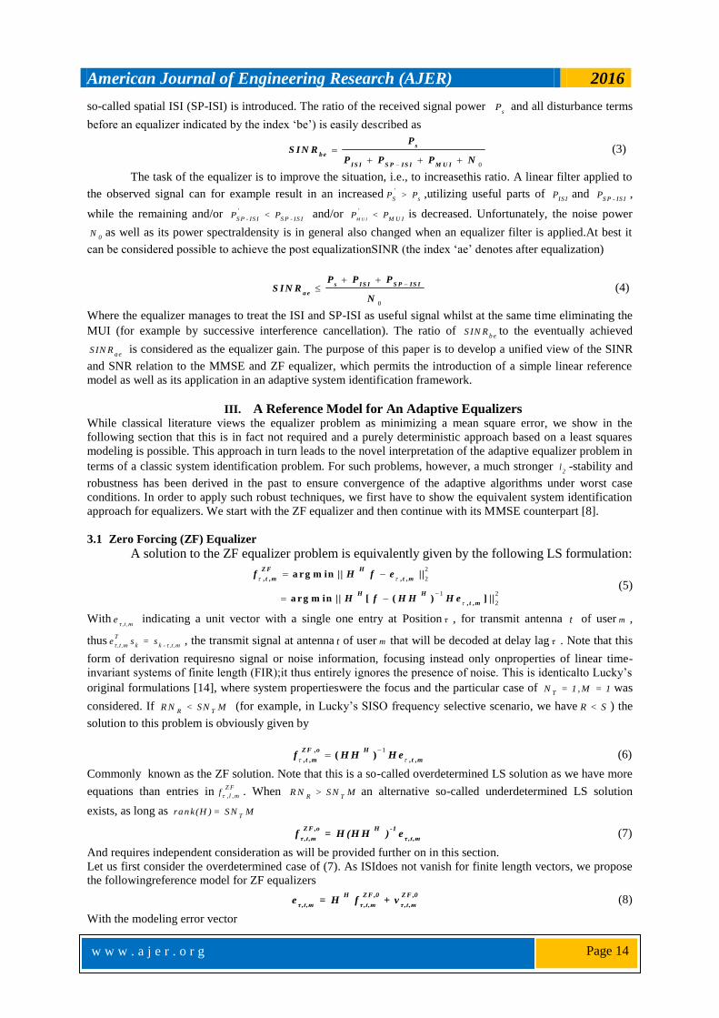
Note that for a toeplitz form channel H we have R < S . A linear equalizer applies an FIR filter f on the received

signal kr so that H

kf r is an estimate of T

k - τ τ ks = e s for the delayed version of ks . A unit vector

0 0 1 0 0 e , , , , , ,

T with a single one at position facilitates the description.

2.2 Single User (SU) Transmission for Frequency Selective MIMO Channels

The transmissions follow the same form as described in equation (5), although with a different

meaning as we transmit overT

N antennas and receive byR

N . Suchmultiple input multiple- outputsystems are

generally referred toasMIMO systems. The transmit vector T

k 1 ,k 2 ,k N ,kTs = s , s ,… , s

is of dimension

T1× N , the

channel matrix H ,and thus the receive vector and the additive noise vector are of dimensionR

1× N .

Here, TN is the number of transmit antennas. As in the previous case, we assume each entry of the transmit

vector to have unit power. Unlike the earlier situation, however, we have to distinguish R T

N > N (under

determined LS solution) and R T

N < N (over determined LS solution). ForR T

N = N both solutions coincide. In

order to detect the various entries of the transmit vectork

s , we again employ a unit vector T

t t k t ,ke : e s = s . Note

however that in contrast to the previous channel model, a set of T

N different vectors t T

e ; t = 1 ,2 ,… , N will be

employed in order to select allT

N transmitted symbols while in the frequency selective SISO case a single

vectorτ

e is sufficient. Early works on linear MIMO equalization can befound in [15] and [16]. Note that

precoding matrices are often applied in particular in modern cellular systems such as HSDPA and LTE. In this

case the concatenation of the precoding matrix and the wireless channel has to be considered as a new

compound channel. Such precoding matrices can also have an impact on the dimension of the transmit vector

ks as in many cases fewer symbols than rank are transmitted at each time instant k . A particular form of this is

given when the precoding matrix shrinks to a vector, in which case we talk about beamforming where only one

symbol stream is transmitted.

2.3 Maximizing SIR and SINR

To understand the vast amount of research and information available on this subject, one has to ask the

question “What is the purpose of an equalizer?” While Lucky‟s original work focused on the SU scenario,

attempting a minimax approach to combat intersymbolinterference (ISI), today we typically view the equalizer

in terms of signal-to-interference ratio (SIR) or signal-to-interference and noise ratio (SINR). If a signal, sayk

s ,

is transmitted through a frequency selective channel, a mixture of ISI, additive noise and signals from other

users multiuser interference (MUI) is received. If signals are transmitted by multiple antennas, then additional



Page 14

so-called spatial ISI (SP-ISI) is introduced. The ratio of the received signal power s

P and all disturbance terms

before an equalizer indicated by the index „be‟) is easily described as

0

s

b e

IS I S P IS I M U I

PS IN R

P P P N (3)

The task of the equalizer is to improve the situation, i.e., to increasethis ratio. A linear filter applied to

the observed signal can for example result in an increased '

S sP > P ,utilizing useful parts of

IS IP and

S P - IS IP ,

while the remaining and/or '

S P - IS I S P - IS IP < P and/or

M U I

'

M U IP < P is decreased. Unfortunately, the noise power

0N as well as its power spectraldensity is in general also changed when an equalizer filter is applied.At best it

can be considered possible to achieve the post equalizationSINR (the index „ae‟ denotes after equalization)

0

s IS I S P IS I

a e

P P PS IN R

N (4)

Where the equalizer manages to treat the ISI and SP-ISI as useful signal whilst at the same time eliminating the

MUI (for example by successive interference cancellation). The ratio of b e

S IN R to the eventually achieved

a eS IN R is considered as the equalizer gain. The purpose of this paper is to develop a unified view of the SINR

and SNR relation to the MMSE and ZF equalizer, which permits the introduction of a simple linear reference

model as well as its application in an adaptive system identification framework.

III. A Reference Model for An Adaptive Equalizers

While classical literature views the equalizer problem as minimizing a mean square error, we show in the

following section that this is in fact not required and a purely deterministic approach based on a least squares

modeling is possible. This approach in turn leads to the novel interpretation of the adaptive equalizer problem in

terms of a classic system identification problem. For such problems, however, a much stronger 2

l -stability and

robustness has been derived in the past to ensure convergence of the adaptive algorithms under worst case

conditions. In order to apply such robust techniques, we first have to show the equivalent system identification

approach for equalizers. We start with the ZF equalizer and then continue with its MMSE counterpart [8].

3.1 Zero Forcing (ZF) Equalizer

A solution to the ZF equalizer problem is equivalently given by the following LS formulation:

2

2

1 2

2

, , , ,

, ,

a r g m in || ||

a r g m in || [ ( ) ] ||

Z F H

t m t m

H H

t m

f H f e

H f H H H e

(5)

Withτ ,t ,m

e indicating a unit vector with a single one entry at Position τ , for transmit antenna t of user m ,

thusT

τ ,t ,m k k - τ ,t ,me s = s , the transmit signal at antenna t of user m that will be decoded at delay lag τ . Note that this

form of derivation requiresno signal or noise information, focusing instead only onproperties of linear time-

invariant systems of finite length (FIR);it thus entirely ignores the presence of noise. This is identicalto Lucky‟s

original formulations [14], where system propertieswere the focus and the particular case of T

N = 1, M = 1 was

considered. If R T

R N < S N M (for example, in Lucky‟s SISO frequency selective scenario, we have R < S ) the

solution to this problem is obviously given by

1

,

, , , ,( )

Z F o H

t m t mf H H H e (6)

Commonly known as the ZF solution. Note that this is a so-called overdetermined LS solution as we have more

equations than entries in, ,

Z F

l mf . When

R TR N > S N M an alternative so-called underdetermined LS solution

exists, as long as T

rank(H ) = SN M

Z F ,o H -1

τ,t,m τ,t,mf = H (H H ) e (7)

And requires independent consideration as will be provided further on in this section.

Let us first consider the overdetermined case of (7). As ISIdoes not vanish for finite length vectors, we propose

the followingreference model for ZF equalizers

H Z F ,0 Z F ,0

τ,t,m τ,t,m τ,t,me = H f + v (8)

With the modeling error vector



Page 15

1

,

, , , ,( ( ) )

Z F o H H

t m t mv I H H H H e (9)

The term ,

, ,

Z F o

t mv models ISI, SP-ISI, and MUI. The larger the equalizer length

RR N , the smaller the ISI, e.g.,

measured in , 2

, , 2| | | |

Z F o

t mv . The cursor position also influences the result.

3.2 Minimum Mean Square Error (MMSE) Equalizer

MMSE solutions are typically derived on the basis of signal and noise statistics [21], e.g., by

M M S E H 2

τ,t,m k k - τ,t,mf = argm in E [| f r - s | ] (10)

However, the linear MMSE solution can alternatively be defined by

M M S E H 2 2

τ ,t ,m τ ,t ,m 2 0 2

1

H H -1 22

0 0 τ ,t ,m 2

f = a rg m in (|| H f - e || + N || f || )

= a rg m in || (H H + N I) [f - (H H + N I) H e ] | | + M M S E

(11)

With an additional term, according to the additive noise variance0

N . We consider here white noise; alternative

forms with colored noise, as originating, for example from fractionally spaced equalizers, is straightforward; one

only has to replace 0

N I withvv

R , the autocorrelation matrix of the noise.

This formulation of the equation (11) has now revealed that the MMSE problem equivalently can be written as a

weighted LS problem with the

T H H -1

τ,t,m 0 τ,t,mM M S E = e [I - H (H H + N I) H ]e (12)

Defines the minimum mean square error. As the term is independent of f , it can thus be dropped when

minimizing equation (11). The well-known MMSE solution is now obviously

M M S E H -1

τ,t,m 0 τ,t,mf = (H H + N I) H e (13)

Similarly to the ZF equalizer, an over determined solution for R N < S N MR T

also exists here.

M M S E ,o H -1

τ,t,m 0 τ,t,mf = H (H H + N I) e (14)

Under white noise both solutions are in fact identicalM M S E ,o M M S E

τ ,t ,m τ ,t ,mf = f , which is very different to the ZF

equalizer. Correspondingly, to thereference model for ZF equalizers in equation (8), we can now alsodefine a

reference model for MMSE equalizers

H M M S E M M S E

τ,t,m τ,t,m τ,t,me = H f + v (15)

With the modeling error

M M S E H H -1

τ,t,m 0 τ,t,mv = (I - H (H H + N I) H )e (16)

Note, however, that unlike in the case of the ZF solution themodeling error is not orthogonal to the MMSE

solution, i.e., M M S E H M M S E

τ ,t ,m τ ,t ,mv H f is not equal to zero. MMSE equalizers are typically designed on the basis of

observations rather than system parameters.Multiplying the signal vector with τ ,t ,m

e we obtain

T M M S E H M M S E H

τ,t,m k k - τ,t,m τ,t,m k τ,t,m ke s = s = f H S + v S (17)

How does a received signal look after such MMSE-equalization? We apply on the observation vector and obtain

M M S E , H M M S E , H M M S E , H

τ ,t ,m k k - τ τ k τ ,t ,m k

M M S Ek - τ k ,t ,m

f r = s - v s + f v

= s + v

(18)

From classic equalizer theory it is well known that the remainingISI energy of the ZF equalizer is smaller than

that ofthe MMSE parts.The weighted LS solution M M S E

τ ,t ,mf of equation (17),applied to the observation vector

kr ,

defines a linear referencemodel in which the desired output signal is k - τ

s , originating from a transmitted signal

over antenna t of user m , corrupted by additive compound noise M M S E

k ,t ,mv . The compound noise is defined by

M M S E ,H

τ ,t ,m kf v as well as by the modeling noise M M S E ,H

τ kv s , defined by the modeling error vector M M S E ,H

τv in

equation (16)



Page 16

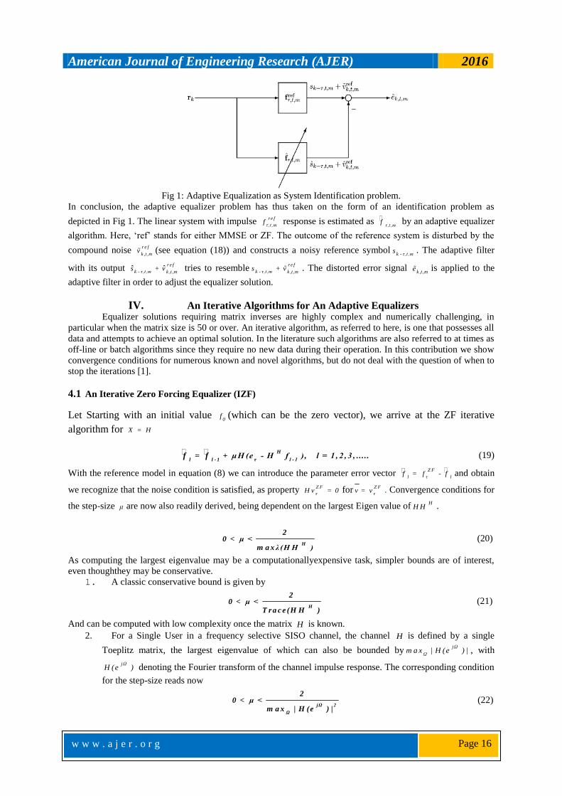
Fig 1: Adaptive Equalization as System Identification problem.

In conclusion, the adaptive equalizer problem has thus taken on the form of an identification problem as

depicted in Fig 1. The linear system with impulse r e f

τ ,t ,mf response is estimated as

τ ,t ,mf by an adaptive equalizer

algorithm. Here, „ref‟ stands for either MMSE or ZF. The outcome of the reference system is disturbed by the

compound noise r e f

k ,t ,mv (see equation (18)) and constructs a noisy reference symbol

k - τ ,t ,ms . The adaptive filter

with its output r e f

k - τ ,t ,m k ,t ,ms + vˆ ˆ tries to resemble

r e f

k - τ ,t ,m k ,t ,ms + v . The distorted error signal

k ,t ,me is applied to the

adaptive filter in order to adjust the equalizer solution.

IV. An Iterative Algorithms for An Adaptive Equalizers Equalizer solutions requiring matrix inverses are highly complex and numerically challenging, in

particular when the matrix size is 50 or over. An iterative algorithm, as referred to here, is one that possesses all

data and attempts to achieve an optimal solution. In the literature such algorithms are also referred to at times as

off-line or batch algorithms since they require no new data during their operation. In this contribution we show

convergence conditions for numerous known and novel algorithms, but do not deal with the question of when to

stop the iterations [1].

4.1 An Iterative Zero Forcing Equalizer (IZF)

Let Starting with an initial value 0

f (which can be the zero vector), we arrive at the ZF iterative

algorithm for X = H

H

τ l - 1l l - 1f = f + μ H (e - H f ), l = 1 , 2 , 3 , ..... (19)

With the reference model in equation (8) we can introduce the parameter error vector Z F

τl lf = f - f and obtain

we recognize that the noise condition is satisfied, as property Z F

τH v = 0 for Z F

τv = v . Convergence conditions for

the step-size μ are now also readily derived, being dependent on the largest Eigen value of HH H .

H

20 < μ <

m a x λ (H H )

(20)

As computing the largest eigenvalue may be a computationallyexpensive task, simpler bounds are of interest,

even thoughthey may be conservative.

1. A classic conservative bound is given by

H

20 < μ <

T ra c e (H H )

(21)

And can be computed with low complexity once the matrix H is known.

2. For a Single User in a frequency selective SISO channel, the channel H is defined by a single

Toeplitz matrix, the largest eigenvalue of which can also be bounded byjΩ

Ωm a x | H (e ) | , with

jΩH (e ) denoting the Fourier transform of the channel impulse response. The corresponding condition

for the step-size reads now

jΩ 2

Ω

20 < μ <

m a x | H (e ) | (22)



Page 17

Such a step-size may be more conservative than the condition in equation (20) but it is also more practical to

find.

In the simulation examples presented the bound so obtained is very close to the theoretical value in equation

(20).

(i)System Mismatch (ii)Relative Error

Fig.2:I t e r a t i v e Zero Forcing Equalizer

Depending upon different step size conditions we have calculated Relative System mismatch and Error. Here as

the number of iterations increases error decreases means we are converging towards desired values of filter

weights.

4.2 An Iterative Fast Convergent An Zero Forcing Equalizer (IF-ZFE)

As the convergenceof the previous equalizer algorithm (Iterative ZF Algorithm) is dependent on the channel

matrix H , the algorithm exhibits much slower convergence forsome channels than for others, even for optimal

step-sizes. Theanalysis of the algorithm shows that the optimal matrix B that ensures fastest convergence is

given by H -1B = [H H ] , which is exactly the inverse whose computation we are attempting toavoid with the

iterative approach. If, however, some a prioriknowledge is present on the channel class (e.g., Pedestrian Bor

Vehicular A), then we can precompute the mean value overan ensemble of channels from a specific class, for

example

H -1 -1

H HE [[H H ] ] = R (23)

In this case, the algorithm updates read

-1 H

H H τl l - 1 l - 1f = f + μ R H (e - H f ); l = 1 , 2 , ..... (24)

Convergence condition for this algorithm will be

H

20 < μ <

m a x λ (H H )

(25)

(i)System Mismatch (ii)Relative Error Fig.3:Fast Convergent of An Iterative Zero Forcing Equalizer



Page 18

(i)IZFE (ii)IF-ZFE

Fig.4:SystemMismatch Comparison ofIZFE v/s IF-ZFE

The convergence speed of above Zero Forcing Equalizer depends upon the channel, for some channels it is

slowly convergent and for others it is fast convergent. For IF-ZFE, We can observe from results that this

algorithm is fast convergent as compared to anIZFEalgorithm as it reaches the desired value in very few

iterations.

4.3 An Iterative Minimum Mean Square Error Equalizer (IM2SE

2)

Let‟s start with our MMSE reference model equation (15), we consider the following update equation

H

τ 0k k - 1 k - 1f = f + μ X (H e - (H H + N I) f ) (26)

We can thus reformulate equation (26) into

H

k 0k - 1 k - 1f = f - μ X (H H + N I ) f (27)

If we select X = I , we can identify H

0B = H H + N I and we find as a condition for convergence that

H

0

20 < μ <

m a x λ (H H + N I) (28)

(i)System Mismatch (ii)Relative Error Fig.5:IterativeMinimumMeanSquareErrorEqualizer

The an IZF Equalizer does not consider channel noise, it cannot deal with noisy channel, and to deal this

problem we designed MMSE Equalizer which considers channel noise in its algorithm for calculating the step

size and Equalizer solution. Here also depending upon different step size conditions we have calculated Relative

System mismatch and Error. Here as the number of iterations increases error decreases means we are converging

towards desired values of filter weights.



Page 19

4.4 An Iterative Fast Convergent Minimum Mean Square Error Equalizer (IF-M2SE

2)

As the convergence of the previous equalizer algorithm (Iterative MMSE Algorithm) is dependent on the

channel matrix H, the algorithm exhibits much slower convergence for some channels than for others, even for

optimal step-sizes. The analysis of the algorithm shows that the optimal matrix B that ensures fastest

convergence is given by H -1B = [H H ] , which is exactly the inverse whose computation we are attempting to

avoid with the iterative approach. If, however, some a priori knowledge is present on the channel class (e.g.,

Pedestrian B or Vehicular A), then we can precompute the mean value over an ensemble of channels from a

specific class, a speedup algorithm is possible with

-1

H H 0X = (R + N I ) (29)

In this case our Fast Convergent MMSE Algorithm will become

-1 H

H H 0 τ 0k k - 1 k - 1f = f + μ (R + N I) (H e - (H H + N I) f ) (30)

The Convergence condition for this algorithm will be

H

0

20 < μ <

m a x λ (H H + N I) (31)

(i)System Mismatch (ii)Relative Error Fig.6:Fast Convergent An Iterative Minimum Mean Square Error Equalizer

(i)IM

2SE

2 (ii)IF- M

2SE

2

Figure7:SystemMismatch Comparison ofIM2SE

2 v/s IF- M

2SE

2

The convergence speed of above IM2SE

2depends on the channel, for some channels it is slowly convergent and

for others it is fast convergent. For IF- M2SE

2, We can observe from results that this algorithm is fast convergent

as compared to aIM2SE

2algorithm as it reaches the desired value in very few iterations. We have also compared

IZF with IM2SE

2, which is shown in the results. From the results, we can observe that the relative Error of

IM2SE

2is less as compared to IZF, because IZF Equalizer can't deal with noisy channels this problem we have

overcome using IM2SE

2 Equalizer which reduces ISI as well as noise power.



Page 20

(i)IM

2SE

2 (ii)IF- M

2SE

2

Figure8:Relative Error Comparison ofIM2SE

2 v/s IF- M

2SE

2

As compared to an IM2SE

2algorithm as it reaches the desired value in very little iteration. We have also

compared an IZF with a n IM2SE

2, which is shown in the results. From the results, we can observe that the

relative Error of a n IM2SE

2isless as compared to an IZF, because an IZF Equalizer can‟t deal with noisy

channels this problem we have overcomeusingIM2SE

2EqualizerwhichreducesISIaswellasnoisepower.

(i)Relative Error IZF (ii)RelativeErrorIM2SE

2

Fig.9:RelativeErrorComparison ofIZFandIM2SE

2Equalizers

In order to perform out theoretical findings, we present selected Matlab examples, we consider a set of seven

channels impulse response of finite length [8] with the length of the channel to be M = 50 for which even the

first four impulse responses have decayed considerably. If we run an iterative receiver (also of 50 taps), the

result for ( 3 )

kh is depicted on the left-hand side (LHS) of Figures, with

0f denoting the ZF solution and

lf

denoting its estimate. Based on the convergence condition in equation (20) it is possible to compute the exact

step-size bound (0.255), given the channel matrix H . Also shown in the figure are the conservative bound in

equation (20), which is the smallest step-size (0.017) in the figure, resulting in the slowest convergence speed

and equation (21), which is just a fraction smaller (0.25 vs. 0.255) than the step-size bound. The average inverse

autocorrelation -1

H HR is computed over all seven channels, and applied in the algorithm‟s updates. This results in

a considerable speed-up in the iterations as proposed and is depicted on the right-hand side (RHS) of Figures.

V. Conclusion Due to an LS approach it is now possible to derive the classical equalizer types with an alternative

formulation, and LS formulation for IZF and a weighted LS formulation for IM2SE

2 equalizers. This in turn

resulted in a linear reference model for both. Based on such a linear reference model, it is possible to derive

iterative forms of equalizers that are robust. Conditions for their robustness were presented, and in particular

ranges for their only free parameter, the step-size, were presented to guarantee robust learning. We have also

compared IZF and IM2SE

2 and IF- M

2SE

2 Equalizers, it is found that IF- M

2SE

2 Equalizer performs better as

compared to IZF and IM2SE

2Equalizer. Simulation example validates our findings.



Page 21

References

[1] Markus Rupp. “Robust design of adaptive equalizers” Signal Processing, IEEE Transactionson, 60(4):1612–1626, 2012. [2] Paul L Feintuch. “Anadaptive r ecu r s i v e LMSfilter”. Proceedings of the IEEE, 64(11):1622–1624, 1976.

[3] C Richard Johnson Jr, Michael G Larimore, PL Feintuch, and N.J.Bershad.“Comments onandadditions toanadaptive

recursiveLMSfilter”. Proceedings oftheIEEE, 65(9):1399–1402, 1977. [4] Markus Rupp and Ali H Sayed.“On the stability andconvergenceofFeintuch‟salgorithmforadaptiveIIRfiltering”.InAcoustics,

Speech,and SignalProcessing, 1995.ICASSP-95, 1995InternationalConferenceo n , volume2,pages1388–1391, 1995.

[5] Markus Ruppand AliHSayed. “Atime-domain f eed b a c k analysisoffiltered- erroradaptive g r a d i e n t algorithms”. Signal Processing, I E E E Transactionson, 44(6):1428–1439, 1996.

[6] Robert Dallinger and Markus Rupp.“A strict stability limit for adaptive gradient type algorithms” In Signals, Systems and

Computers, 2 0 0 9 Conference Record o f the Forty-Third Asilomar Conference on, 1370–1374.IEEE, 2009. [7] Markus Rupp.“Pseudo a f f in eprojection algorithmsrevi s i t ed : robustness an d stability a n a l y s i s ” SignalProcessing,

I E E E T r a n s a c t i o n s o n , 5 9 (5):2017–2023, 2011.

[8] MarkusRupp. “Convergencepropertiesofadaptiveequalizeralgorithms” Signal Processing, IEEE Transactionson, ( 6): 2562 – 2574, 2011.

[9] AliHSayed andMarkusRupp . “Error-energy bounds f o r adaptive gradient algorithms” Signal Processing, IEEE Transactions

,44(8):1982–1989,1996. [10] A.H.Sayed andM Rupp. “Robustness issuesin adaptive f i l t e r s ” The DSPHandbook.

[11] RWLucky. “Automaticequalization f o r digital communication” BellSystem Technical Journal,44(4):547–588,1965.

[12] Dominique Godard.“Self-recovering equalization a n d carrier tracking i n two-dimensional da ta c o m m u n i c a t i o n systems”IEEET r a n s a c t i o n s on,28(11):1867–1875,1980.

[13] Simon S Haykin. Adaptive filter theory. Pearson Education India, 2007.

[14] Bjorn A Bjerke and John G Proakis. “Equalizationanddecodingformultiple- input multiple-outputwirelesschannels”. EURASIP Journal onAppliedSignal Processing, 2002(1):249–266, 2002.

[20] Shahid U H Qureshi. “Adaptive equalization”. Proceedings of the IEEE, 73(9):1349–1387,1985.

[21] John G Proakis. “Intersymbol Interference inDigitalCommunication Systems”. WileyOnlineLibrary, 2001.

1Sayed Shoaib Anwar,was born on 15thJune 1982 in Nanded, Maharshtra, India, He received his bachelor of

Engineering from Dr. B.A.M. University, in 2005.He completed his Master degree in 2007 from S.G.G.S.I.E&T.

He started his doctoral studies in the area Multicarrier Communication. He is having the research interest in the field of wireless communication, Multicarrier Communication and OFDM system. He Published more then14

papers in different journals and [email protected]

Dr. D. Elizabeth Rani, She is recently working as Professor & Head in Electronics and Instrumentation

Engineering department, GIT-GITAM, Visakhapatnam, India. She received her bachelor of Engineering in 1982, Master degree in 1984 from and Doctorate in the field of Communication in 2003.Her area of specialization is

Signal processing. She published more than 20 research papers in different Journals and conferences.

[email protected]

Dr. S.G.Kahalekar,he worked as a Professor,SGGSI of Engg. & Tech,Nanded.He received his bachelor of Engineering in 1975. He completed his Master degree in 1977 from IIT, Kharagpur. He completed his Doctorate

in the field of Biomedical in 2008.He has more than 40 years of experience in research field. He received

different awards in research field. [email protected]

Dr. Syed Abdul Sattar, he is currently working asDean, Royal Institute of Technology & Science, he is having the qualification B.Tech. (ECE), M.Tech. ,(DSCE), Ph.D.(ECE), Ph.D. (CS), his area of research is Electronic

Communications and Computer Engineering. He has more than 25 years of experience in research. He published

more than 150 research papers in different journals and [email protected]

mailto:[email protected]




Documents

A Novel Convergence Approach for an Adaptive …03)/C0503012021.pdfLinear equalizers were designed either on the deterministic ZF approach for equalizers of ZF type or on the stochastic