Genetic Epidemiology 36: 36–47 (2012)

A Novel Bayesian Graphical Model for Genome-Wide Multi-SNPAssociation Mapping

Yu Zhang1�

1Department of Statistics, The Pennsylvania State University, University Park, Pennsylvania

Most disease association mapping algorithms are based on hypothesis testing procedures that test one variant at a time.Those methods lose power when the disease mutations are jointly tagged by multiple variants, or when gene-geneinteraction exist. Nearby variants are also correlated, for which procedures ignoring the dependence between variants willinevitably produce redundant results. With a large number of variants genotyped in current genome-wide diseaseassociation studies, simultaneous multivariant association mapping algorithms are strongly desired. We present a novelBayesian method for automatic detection of multivariant joint association in genome-wide case-control studies. Our methodhas improved power and specificity over existing tools. We fit a joint probabilistic model to the entire data and identifydisease variants simultaneously. The method dynamically accounts for the strong linkage disequilibrium (LD) betweenvariants. As a result, only the primary disease variants will be identified, with all secondary associations due to LD effectsfiltered out. Our method better pinpoints the disease variants with improved resolution. The method is alsocomputationally efficient for genome-wide studies. When applied to a real data set of inflammatory bowel disease (IBD)containing 401,473 variants in 4,720 individuals, our method detected all previously reported IBD loci in the same data, andrecovered two missed loci. We further detected two novel interchromosome interactions. The first is between STAT3 andPARD6G, and the second is between DLG5 and an intergenic region at 5p14. We further validated the two interactions in anindependent study. Genet. Epidemiol. 36: 36–47, 2012. r 2011 Wiley Periodicals, Inc.

Key words: disease association mapping; Bayesian graph; linkage disequilibrium; Markov chain Monte Carlo

Additional Supporting Information maybe found in the online version of this article.Contract grant sponsor: NIH; Contract grant number: R01-HG004718.�Correspondence to: Yu Zhang, Department of Statistics, The Pennsylvania State University, 421A Thomas Building, University Park,PA 16802. E-mail: yuzhang@stat.psu.eduReceived 28 July 2011; Revised 20 September 2011; Accepted 5 October 2011Published online 29 November 2011 in Wiley Online Library (wileyonlinelibrary.com/journal/gepi).DOI: 10.1002/gepi.20661

INTRODUCTION

Genome-wide association study (GWAS) for complexdiseases has become routine in recent years [WTCCC,2007]. The goal is to identify potential locations in thegenome containing mutations that may affect the risk ofcomplex diseases. Single nucleotide polymorphism (SNP)is a typical marker used in GWAS. A common approach incase control setting is to compare the SNP genotypedistribution between the affected and the unaffectedindividuals. If a disease mutation occurs at a locus in thegenome, which is typically unobserved, its nearby SNPswill demonstrate association with the disease due tolinkage disequilibrium (LD). LD can be understood asdependence in statistical sense, and LD diminishes overdistance. It is thus expected that SNPs genotyped in aGWAS can capture the information of unobserved diseasemutations nearby. The genotyped SNPs are called taggingSNPs. Intuitively, with more SNPs genotyped in a GWAS,the more likely that a disease mutation is tagged orobserved, and thus increases the power of GWAS. Theproblem is however complicated by the increasing numberof SNPs, such as the additional computation burden andthe issues created by LD among densely genotyped SNPs.

Many current association mapping approaches onlyfocus on testing single-SNP association with the disease.Despite their simplicity, single-SNP methods inevitablylose power when interaction association exists betweenSNPs [Moore and Williams, 2002; Marchini et al., 2005;Zhang and Liu, 2007]. Single-SNP methods also performpoorly when the disease mutations are jointly captured bymultiple tagging SNPs [Zhang et al., 2002; Kuno et al.,2004; de Bakker et al., 2005], which is common due to thenature of the tagging SNP selection criteria. A few recentstudies [Cirulli and Goldstein, 2010] further suggestedthat the risk of complex traits may be attributable torare mutations, in which case single-SNP methods will bepowerless regardless of how many tagging SNPs aregenotyped. Owing to these reasons, advanced statisticalmethods for automatic detection of multi-SNP associationmapping are strongly desired [Cordell, 2009]. Testingmulti-SNP associations is an interesting and importantproblem, yet the task is very difficult because there are toomany possible SNP combinations to be explored in thegenome-wide scale. A few computationally efficientmulti-SNP mapping algorithms have emerged recently,demonstrating that whole-genome multi-SNP associationmapping is computationally feasible, and at the same timestatistically powerful [Marchini et al., 2005; Zhang and Liu,

r 2011 Wiley Periodicals, Inc.

2007; Schwartz et al., 2008; Wu et al., 2009; Wan et al., 2010;Zhang et al., 2011; Liu et al., 2011].

Even if one is only interested in single-SNP association,most existing methods have problems when many SNPs instrong LD are genotyped in a region. In particular, LD cancreate a large number of secondary disease associationsaround a true disease mutation. Most methods usehypothesis testing procedures [Marchini et al., 2005; Wanet al., 2010; Liu et al., 2011] to test each SNP or SNP setseparately in a stepwise manner, ignoring the LD effects.As a result, they are likely to report a large number ofredundant association, with biased effect estimates, due tomissing important variants in their tests. Distinct from thehypothesis testing procedures, there are also joint diseasemapping approaches [Zhang and Liu, 2007; Schwartzet al., 2008; Wu et al., 2009; Zhang et al., 2011] that fit asingle model to all SNPs simultaneously, and detect SNPassociation conditioning on all other SNPs. Although jointmapping approaches are potentially more powerful androbust than hypothesis testing approaches, many existingalgorithms are computationally demanding for large-scalestudies, and most methods cannot sufficiently account forthe complex LD effects among dense SNPs. We show inour simulation study that insufficient modeling of LDcould substantially increase the analysis complexity andcompromise the disease mapping results.

In this article, we introduce a novel Bayesian graphicalmethod, called BEAM3, for large-scale association mapping.BEAM3 simultaneously detects single-SNP, multilocal-SNP,and long-distance SNP-SNP interaction associations.BEAM3 is particularly advantageous for analyzing a largenumber of SNPs with possibly strong LD. There are twomajor improvements of BEAM3 compared with existingmethods and our previous BEAM models [Zhang and Liu,2007; Zhang et al., 2011]. First, multi-SNP associations andhigh-order interactions have exponentially growing modelcomplexity, for which saturated models are powerless. Thenew method detects flexible interaction structures usinggraphs, which substantially reduces the multi-SNP modelcomplexity and hence improves the power. Second, BEAM3achieves computational efficiency for GWAS by construct-ing only the disease association graphs, while avoidinginference of the unknown huge and complicated depen-dence graph for genome-wide SNPs. The latter is typical inpractice but is only applicable to much smaller studies.Third, the method uses a flexible graph structure toimplicitly account for the unknown LD among SNPs, suchthat only the primary disease associations will be reported.All secondary associations due to LD effects will be filteredout. BEAM3 therefore produces cleaner results with greatlyimproved mapping sensitivity and specificity, which willgreatly simplify the downstream analysis. Our new methodis well suited in a Bayesian framework. Various diseaseSNPs and interactions are automatically evaluated usingregularized probabilities, with minimum input requirementfrom the user. Biological expert information can also beeasily incorporated into our model as priors.

With recent advance in high-throughput sequencingtechnologies [Metzker, 2010], it becomes cost-effective togenotype millions of SNPs in GWAS. It is thus stronglydesirable to develop advanced statistical methods, withunified and flexible single-SNP and multi-SNP models, toimprove the power of detecting subtle disease associationsand interactions. We performed large-scale simulationstudy to demonstrate the superior performance of BEAM3

compared with several existing methods, including pena-lized regression methods, machine learning methods, andour previous Bayesian partition methods. We furtherapplied BEAM3 to a GWAS data set of inflammatorybowel disease (IBD) from WTCCC [2007]. We successfullyidentified all previously reported IBD loci from this dataand recovered two missed loci. We also identified twolocal joint-tagging association at known IBD loci, andtwo interchromosome interactions. We validated the twointerchromosome interactions in an independent study.

MATERIAL AND METHODS

NOTATION

Let Y denote the binary disease status of case controlindividuals and X denotes the SNP data to be tested forassociation with Y. Our approach is to model thedistribution of X given Y. Since not all SNPs in X areassociated with Y, the goal is to select a subset of SNPs in Xthat are most likely associated with Y either marginally orjointly with other SNPs. It is extremely complicated toconsider all possible interaction models among all SNPs.We therefore restrict our method to only detect saturatedinteractions of SNPs within a selected subset of SNPs(called cliques) and the pairwise interaction betweencliques. That is, high-order interactions are allowed inour model as interactions within cliques and pairwiseinteraction between cliques. We first define our notations:

* Y ¼ ðy1; . . . ; yNÞT: the binary disease status of N

individuals;* X ¼ ðx1; . . . ; xLÞ: L SNPs, where each xi is a vector of

genotypes in N individuals;* I ¼ ðI1; . . . ; ILÞ: vector of L indicators, with Ii 5 1

indicating SNP xi is associated with Y, and 0 otherwise;* X1: set of SNPs with indicator Ii 5 1, i.e., disease-

associated SNPs;* C ¼ ðc1; . . . ; cKÞ: partition of SNPs in X1 into K non-

overlapping cliques;* D ¼ fdijg1�ioj�K: K choose two indicators, with dij 5 1

indicating interaction between cliques ci and cj, and 0otherwise.

* G 5 (C,D): an undirected graph built on SNPs in X1,called disease graph.

PROBABILITY FUNCTIONS BUILT ON AGRAPH

We first describe the probability functions used in ourgraphical model. The functions are designed for casecontrol studies with dichotomous disease outcome andcategorical genotypes. Given a collection Xc of k SNPs,there are 3k possible genotype combinations (genotype isthe observed value at a SNP in an individual, and thereare three possible genotype values). Let ni, mi denote thenumber of genotype combination i observed in cases andcontrols, respectively, and let pi, qi denote their frequencies,respectively. We write

PrðXcjYÞ ¼Y3k

i¼1

pni

i qmi

i :

37Novel Bayesian Graphical Model

Genet. Epidemiol.

Since pi, qi are unknown, we assume a Dirichlet prior forpi, qi with hyper-parameter ai ¼ 1:5=3k, and we integrateout pi, qi to obtain

PrðXcjYÞ ¼Y3k

i¼1

Gðni1aiÞGðmi1aiÞ

GðaiÞ2

GðaÞ2

GðNc1aÞGðNu1aÞ; ð1Þ

where Nc ¼P3k

i¼1 ni, Nu ¼P3k

i¼1 mi denote the case andcontrol sample sizes, respectively, and a ¼

P3k

i¼1 ai ¼ 1:5.Formula (1) models the data observed in cases and

controls separately, which is appropriate if SNPs in Xc areassociated with the disease Y. On the other hand, if SNPsin Xc are not associated with the disease, we should havepi 5 qi for all i ¼ 1; . . . ; 3k, and hence

PrðXcÞ ¼Y3k

i¼1

Gðni1mi1aiÞ

GðaiÞ

GðaÞGðNc1Nu1aÞ

: ð2Þ

A joint probability function of all SNPs in X1 (the set ofdisease-associated SNPs) can be modeled by an undirectedacyclic graph G 5 (C, D) conditioning on Y as

PAðX1jY;GÞ ¼YKi¼1

PrðxcijYÞ

Yfi;j:dij¼1g

Prðxci1cjjYÞ

PrðxcijYÞPrðxcj

jYÞ; ð3Þ

where each term in (3) is defined in (1). A justification offormula (3) can be found in Online Supplementary Material.

Correspondingly, if we assume that the set of SNPs in X1

are not associated with Y, we can model X1 given a(different) graph G

0

as

P0ðX1jG0Þ ¼

YKi¼1

PrðxciÞY

fi;j:d0ij¼1g

Prðxci1cjÞ

PrðxciÞPrðxcj

Þ; ð4Þ

where each term in (4) is defined in (2).

CHOICE OF PRIOR DISTRIBUTIONS

We specify the prior distribution of SNP membershipsI by a product of independent Bernoulli probabilities,

i.e., PrðIi ¼ 1Þ ¼ 1� PrðIi ¼ 0Þ ¼ p and PrðIÞ ¼QL

i¼1 PrðIiÞ ¼

pjIjð1� pÞL�jIj, where jIj ¼P

i¼1;...;L Ii. By default, we choose

p ¼ 10L , and a larger p will help detecting weaker associa-

tions. It is also possible to specify PrðIi ¼ 1Þ according tosome biological knowledge, e.g., functional potential ofeach SNP. Given I (and hence X1), we specify the priordistribution of a clique partition C of SNPs in X1 by aPitman-Yor process [Pitman and Yor, 1997]. AssumeX1 ¼ ðx1; . . . ; xpÞ. Let Ci ¼ ðc1; . . . ; cKi

Þ denote a partitionof x1; . . . ; xi into Ki non-verlapping cliques. Let nk denotethe number of SNPs in the kth clique. The probability ofassigning a new SNP xi11 into one of the existing cliques is

Prðxi11 2 ckjCi; IÞ ¼nk � b

i1a;

and the probability of assigning xi11 into a new clique is

Prðxi11 2 cKi11jCi; IÞ ¼a1Kib

i1a:

Here, a40 and b 2 ½0; 1Þ are two hyperparameters in thePitman-Yor process, with b5 0 yielding the standardDirichlet process. By default, we let a5 10 and b5 0.5,where larger a and b will favor more cliques. UsingPitman-Yor process in clique partition allows us to

determine the number of cliques probabilistically. GivenI and C, we specify the prior distribution of interactionindicators D between cliques by a product of independentBernoulli probabilities, i.e., Prðdij ¼ 1Þ ¼ 1� PrðdijÞ ¼ pD

and PrðDjI;CÞ ¼Q

ioj PrðdijÞ. By default, we let pD ¼ 0:1,

where a larger pD will help detecting weaker interactions.

THE JOINT PROBABILITY MODEL

We write the joint probability function of all SNPs X,disease status Y, and parameters (I, G) as

PrðX;Y;G; IÞ ¼ PrðXjY;G; IÞPrðYÞPrðGjIÞPrðIÞ; ð5Þ

where Pr(Y) denotes the distribution of disease status,Pr(G|I) denotes the prior distribution of G given I, and Pr(I)denotes the prior distribution of SNP indicators. Note thatour model is retrospective, i.e., we define the distribution ofSNPs conditioning on the disease information.

We next define PrðXjY;G; IÞ in the form

PrðXjY;G; IÞ ¼PAðX1jY;GÞP0ðXjX1;Y;GÞ

¼PAðX1jY;GÞ

P0ðX1jY;GÞP0ðXjY;GÞ

¼PAðX1jY;GÞ

P0ðX1ÞP0ðXÞ

/PAðX1jY;GÞ

P0ðX1Þ:

ð6Þ

Here, PA( � ) denotes a probability function of X1 underthe disease association hypothesis, and its form is givenby (3). P0( � ) denotes a baseline probability function (tobe defined later) of X1 under the null hypothesis of noassociation. In (6), the first line is our definition; the secondand the third line are due to the independence assumptionbetween unassociated SNPs and disease information(Y, G), under the null hypothesis. We define the nullmodel P0(X) to be invariant with respect to G and I, andthus we can treat P0(X) as a constant in our algorithm,yielding the last line of (6).

Our parameters of interest are the disease graph G andthe SNP membership I, where X1 is uniquely determinedby I. Plugging (6) back into (5), we obtain

PrðX;Y;G; IÞ /PAðX1jY;GÞ

P0ðX1ÞPrðGjIÞPrðIÞ: ð7Þ

It is shown in (7) that we avoid explicitly modeling thecomplicated dependence of all SNPs, except for a fewdisease-associated SNPs. The total number of genome-wide SNPs could be in millions, modeling the dependenceof which is computationally formidable. The numberof true and detectable disease SNPs, however, is oftensmall. As a result, our method saves a substantial amountof computation by avoiding explicit modeling of SNPdependence.

The choice of the baseline function P0( � ) in (6) underthe null hypothesis is critical. A simple Markov chain or aLD-block model cannot fully account for the complicateddependence among SNPs. Simple models only work whenthe disease models under the alternative hypothesis areequally restrictive. If a null model is overly simplisticcompared with the disease graph model, numerous false-positive interactions will be produced merely due to itsover-simplicity. We define

38 Zhang

Genet. Epidemiol.

P0ðX1Þ ¼X

G0

P0ðX1jG0ÞPrðG0Þ; ð8Þ

where P0ðX1jG0Þ is defined in (4). Here, we use graphsG0

(different from G) to define the baseline model, whichcan capture the unknown LD among SNPs. We do notinfer G

0

in practice, and thus we sum over all possible G0

.

MARKOV CHAIN MONTE CARLO SAMPLING

We iteratively sample the SNP membership variable Iand the disease graph G from model (7). To update theindicator Ii of SNP i, let X1 and G denote the current setof disease SNPs and the disease graph, respectively,excluding SNP i. We add SNP i into the disease graph toobtain a new set of disease SNPs xi1X1, and a new diseasegraph G1i, conditioning on X1 and G, by calculating

g¼Prðxi1X1;Y;G; Ii¼1Þ

PrðX1;Y;G; Ii¼0Þ¼

PG1i

PAðxi;G1ijX1;Y;GÞPrðIi¼1Þ

P0ðxijX1ÞPrðIi¼0Þ:

ð9Þ

We then sample Ii 5 1 with probability g=ð11gÞ, andIi 5 0 otherwise. Intuitively, if SNP i is more likely to begenerated from the disease association model PA( � ) thanfrom the baseline model P0( � ), we will have g41 and thusthe SNP is likely to be added into X1. On the other hand, ifSNP i is sufficiently explained by the disease SNPs in X1

under the baseline model, i.e., it is explained by LD withSNPs that are already selected in X1, then PA( � ) will besmaller than P0( � ). As a result, go1 and thus the SNPtends not to be selected. That is, LD effects areautomatically accounted for by P0( � ), and this occurs ifand only if we update a SNP’s group membership,without any upfront computation.

Formula (9) involves computing

P0ðxijX1Þ ¼X

G0

� XfG0

1i:G0

1i�G0g

P0ðxi;G01ijX1;G

0Þ

�P0ðG

0jX1Þ;

where G01i denotes a graph of all SNPs in X1 and SNP i,and G

0

denotes a subgraph of G01i excluding SNP i. Inpractice, we generate many random samples of G

0

,denoted by G01; . . . ;G

0m, from the distribution PrðG0jX1Þ,

and we approximate P0ðxijX1Þ by

P0ðxijX1Þ ¼1

m

Xm

j¼1

XfG0

1i:G0

1i�G0

jg

P0ðxi;G01ijX1;G

0jÞ: ð10Þ

To further improve the computation speed, we utlize anapproximate sampling procedure. In each iteration, wesimply let Gj0 ¼ G in (10). That is, rather than sampling G

0

,we directly use the current disease graph G, excludingSNP i, as the dependence graph G

0

in (10). This step candramatically improve the computation speed, although thesampling results will be biased. In all simulation studieswe have checked, the bias produced by this approximatesampling step is very small, yet it substantially improvesthe computation speed by magnitudes. We therefore usethis approximate sampling procedure as a tool to firstscreen for candidate SNPs in genome-wide scale. We thenresample from the full model to estimate the true posteriordistribution of the candidate SNPs.

To further update the disease graph including the cliquepartition C and the interaction indicator D, we sample G1i,

conditioning on the set of SNPs xi1X1 and the subgraph Gexcluding xi, from the distribution

PrðG1ijxi1X1;Y;GÞ ¼PAðxi1X1;G1ijY;GÞPrðG1ijGÞPG1i

PAðxi1X1;G1ijY;GÞPrðG1ijGÞ

¼PAðG1ijxi1X1;Y;GÞ:

ð11Þ

In practice, it is likely that the above sampling algorithmis trapped in a local mode. This is a common problem ofMCMC algorithms. One possible solution is to implementadvanced sampling schemes to achieve better mixing ofthe Markov chains. Alternatively, we suggest running theprogram several times independently and then check if theestimated posterior probabilities are in agreement acrossmultiple runs. In a few cases we checked in our simulationstudy and in the real data analysis, we found that ouralgorithm converged within a hundred iterations.

RESULTS

SIMULATION STUDY

We performed simulation study to evaluate the perfor-mance of BEAM3. We used HAPGEN [WTCCC, 2007] tosimulate a large pool of individuals from the HapMapPhase II sample of European ancestry (CEU, parentalindividuals only) [The International Hapmap Consortium,2005]. There are 2.7 million common SNPs in the HapMapPhase II CEU data, and thus the SNP density is about oneSNP per kb. From the simulated pool of individuals, werandomly sampled cases and controls according to thefollowing logistic regression model:

logitðpÞ ¼ 0:5X110:5X210:5X31X4X5

1X6X711:5X8X9X101c;

where p denotes the probability of disease, and theconstant c relates to disease prevalence. c is not used in oursimulation, because we used a retrospective simulationprocedure with fixed numbers of cases and controls. Inparticular, given a number of case and control individuals,we first calculate a joint genotype frequency of all diseaseSNPs in cases and controls, respectively, based on theabove logistic regression model. We then sample fromthe large pool of individuals according to the diseasegenotype frequency. More details of our simulationprocedure can be found in Zhang and Liu 2007.

Our disease model contains 10 disease SNPs, includingthree marginally associated SNPs X1, X2, X3, two 2-wayinteractions (X4, X5), (X6, X7), and one 3-way interaction(X8, X9, X10). Each SNP takes value in f0; 1; 2g, denoting theminor allele counts at the SNP in each individual. Notethat our choice of using a logistic regression model andcoding SNPs by the minor allele counts does not favor ourmethod.

Each simulated data set contained 10,000 SNPs in 1,000cases and 1,000 controls. All SNPs are distributed in fiverandomly selected regions (cover 10 Mb) in the genome.The 10 disease SNPs were randomly selected from the fiveregions, with a preference giving to SNPs with a desiredminor allele frequency (MAF). The distribution of the 10disease SNPs is summarized in Table I. We generated 50data sets for each disease MAF 5 0.05, 0.1, 0.2, respectively.We also calculated the effect sizes of each disease SNP in

39Novel Bayesian Graphical Model

Genet. Epidemiol.

the simulated data. Of the main effect SNPs (X1, X2, X3),their median effect size is 0.626, 0.590, 0.623 forMAF 5 0.05, 0.1, 0.2, respectively. Of the 2-way interactionSNPs (X4�X7), their median (main) effect size is 0.138,0.300, 0.692, respectively. Of the 3-way interaction SNPs(X8, X9, X10), their median (main) effect size is 0.026, 0.149,0.536, respectively.

We compared BEAM3 with five existing algorithms:ChiSq, Mendel [Wu et al., 2009], RandomJungle [Schwartzet al., 2008], BEAM1 [Zhang and Liu, 2007], and BEAM2[Zhang et al., 2011]. ChiSq is a standard 2� 3 contingencytable test on the genotype counts, which we use tobenchmark the performance of single-SNP tests. Mendel[Wu et al., 2009] is a software package that implements theLASSO penalized regression method [Tibshirani, 1996].Mendel allows detecting both main effects and interactioneffects of SNPs. We ran Mendel in two ways: (1) detectingsingle SNP association only, and (2) detecting both singleSNP and pairwise interaction. We hereafter name thetwo approaches as Mendel-Single and Mendel-Pairwise,respectively. RandomJungle [Schwartz et al., 2008] is amachine learning algorithm that constructs trees to classifyindividuals as affected vs. normal, and evaluates theimportance of SNPs with respects to classification accu-racy. BEAM1 [Zhang and Liu, 2007] is our first Bayesianpartition model for interaction mapping, which utilizes afirst-order Markov chain to account for LD betweenadjacent SNPs. BEAM2 [Zhang et al., 2011] improvesupon BEAM1 by utilizing a LD-block model to capturethe block-like dependence among SNPs. Here we demon-strate that, for dense SNPs, both BEAM1 and BEAM2 areinadequate in modeling strong LD. In addition, BEAM1and BEAM2 only allows detecting one interaction at atime, which loses power when multiple interactions exist.

POWER COMPARISON

We first compared the power of all methods using a plotsimilar to the receiver operating characteristic curve. With-out referring to statistical significance, we define the powerof each program as the fraction of disease SNPs captured bythe top-ranked SNPs. A disease SNP is ‘‘captured’’ if thereis at least one top-ranked SNP within 5 kb to either side ofthe disease SNP. We checked the results using differentwindow sizes, and the conclusion remained the same (anexample using 50-kb window can be found in OnlineSupplementary Material). SNP ranking was obtained fromthe outputs of each program. In particular, we ranked SNPsby the posterior probabilities output by BEAM3, BEAM1,and BEAM2, the P-values by Mendle-Single and Mendel-Pairwise, the importance score by RandomJungle, and thechi-square statistics by ChiSq, respectively.

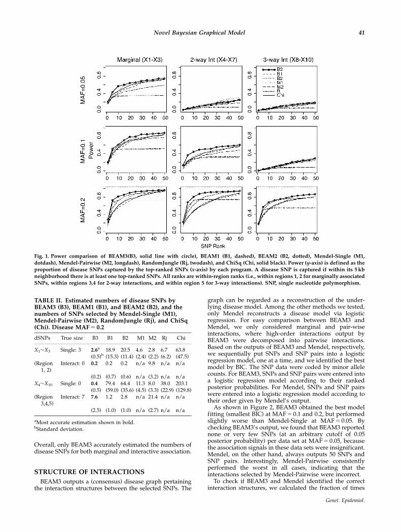
As shown in Figure 1, BEAM3 performed the bestamong all methods for detecting both marginal associa-tions (first column in Fig. 1) and 2-way and 3-wayinteractions (second and third columns in Fig. 1). Amongthe other programs, RandomJungle yielded good powerfor detecting 3-way interactions at MAF 5 0.2. Mendel

(-Single and -Pairwise) yielded good power in the top 10SNPs selected by LASSO penalized regression, yet itspower remained almost flat when more top SNPs areincluded. This suggests that Mendel only detected aportion of the 10 disease SNPs (by default, we let Mendelselect 50 best SNPs or SNP pairs). BEAM1 and ChiSq (andBEAM2 at MAF 5 0.2) yielded relatively low power thanother methods. This is expected, because BEAM1 andChiSq did not sufficiently account for LD, such that theirtop-ranked SNPs are mostly clumped around just a fewstrongest associations. Overall, BEAM3 outperformed theother methods in almost all cases, except for the interac-tions at MAF 5 0.05, which are too weak to be detectable.

NUMBER OF PRIMARY DISEASE SNPS

Using the output of BEAM3, we can estimate thenumber of primary disease SNPs (as oppose to secondaryassociation created by LD) by summing over all SNPs theestimated posterior probabilities of marginal and interac-tion associations. Although BEAM1 and BEAM2 alsooutput posterior probabilities, they tend to over-estimatethe number of disease SNPs due to LD. We show inTable II the estimated numbers of disease SNPs byBEAM3, BEAM1 and BEAM2, from the simulated datasets at MAF 5 0.2. In these data sets, the truth is threemarginal SNPs and seven interacting SNPs. The otherprograms, Mendel, RandomJungle and ChiSq, do notestimate the number of disease SNPs. We insteadcomputed the numbers of single SNPs and pairwiseinteractions selected by Mendel using Bayesian informa-tion criterion (BIC) [Diciccio et al., 1997], and the numberof significant SNPs by RandomJungle and ChiSq, respec-tively.The significance cutoff was estimated by permuta-tion at the 0.05 level. We choose MAF 5 0.2 because theassociation signals in this scenario are strong anddetectable, such that redundancy in SNP detection canbe directly observed as over-estimation of the number ofdisease SNPs. The results for MAF 5 0.05 and 0.1 can befound in Online Supplementary Material, for which the datahowever have weak signals and thus the results areconfounded by missing true SNPs.

As shown in Table II, BEAM3 consistently obtained themost accurate estimates of the numbers of disease SNPsfor both marginal and interaction association. In compar-ison, BEAM1 and BEAM2 substantially overestimated thenumber of marginal associations due to LD effects. Theyalso underestimated the number of interacting SNPs,because they both used a saturated interaction model,and they only detect one interaction at a time. AmongMendel, RandomJungle and ChiSq, Mendel obtained thebest shrinkage (fewest number) of SNP selection, after BIC.In contrast, ChiSq had no shrinkage at all, i.e., allmarginally significant SNPs are reported including pri-mary and secondary associations, 20�30 times larger thanthe true numbers. The number of SNPs selected byMendel, however, still differ significantly from the truth.For instance, Mendel-Pairwise (which allowed both inter-action and main effects) reported an average of 9.8 SNPsinvolved in pairwise interactions in regions (1, 2), wherethe regions only contained marginal associations. Mendel-Pairwise also reported an average of 8.0 SNPs involved inmarginal associations in regions (3, 4, 5), where the regionsonly contained interaction associations. This result sug-gested that Mendel only selected a suboptimal set of SNPs.

TABLE I. Disease SNP distribution in five regions

Region 1 2 3 4 5

Number of SNPs 1,000 2,000 2,000 2,000 3,000Disease SNPs X1 X2,X3 X4,X5 X6,X7 X8,X9,X10

40 Zhang

Genet. Epidemiol.

Overall, only BEAM3 accurately estimated the numbers ofdisease SNPs for both marginal and interactive association.

STRUCTURE OF INTERACTIONS

BEAM3 outputs a (consensus) disease graph pertainingthe interaction structures between the selected SNPs. The

graph can be regarded as a reconstruction of the under-lying disease model. Among the other methods we tested,only Mendel reconstructs a disease model via logisticregression. For easy comparison between BEAM3 andMendel, we only considered marginal and pair-wiseinteractions, where high-order interactions output byBEAM3 were decomposed into pairwise interactions.Based on the outputs of BEAM3 and Mendel, respectively,we sequentially put SNPs and SNP pairs into a logisticregression model, one at a time, and we identified the bestmodel by BIC. The SNP data were coded by minor allelecounts. For BEAM3, SNPs and SNP pairs were entered intoa logistic regression model according to their rankedposterior probabilities. For Mendel, SNPs and SNP pairswere entered into a logistic regression model according totheir order given by Mendel’s output.

As shown in Figure 2, BEAM3 obtained the best modelfitting (smallest BIC) at MAF 5 0.1 and 0.2, but performedslightly worse than Mendel-Single at MAF 5 0.05. Bychecking BEAM3’s output, we found that BEAM3 reportednone or very few SNPs (at an arbitrary cutoff of 0.05posterior probability) per data set at MAF 5 0.05, becausethe association signals in these data sets were insignificant.Mendel, on the other hand, always outputs 50 SNPs andSNP pairs. Interestingly, Mendel-Pairwise consistentlyperformed the worst in all cases, indicating that theinteractions selected by Mendel-Pairwise were incorrect.

To check if BEAM3 and Mendel identified the correctinteraction structures, we calculated the fraction of times

Fig. 1. Power comparison of BEAM3(B3, solid line with circle), BEAM1 (B1, dashed), BEAM2 (B2, dotted), Mendel-Single (M1,

dotdash), Mendel-Pairwise (M2, longdash), RandomJungle (Rj, twodash), and ChiSq (Chi, solid black). Power (y-axis) is defined as theproportion of disease SNPs captured by the top-ranked SNPs (x-axis) by each program. A disease SNP is captured if within its 5 kb

neighborhood there is at least one top-ranked SNPs. All ranks are within-region ranks (i.e., within regions 1, 2 for marginally associated

SNPs, within regions 3,4 for 2-way interactions, and within region 5 for 3-way interactions). SNP, single nucleotide polymorphism.

TABLE II. Estimated numbers of disease SNPs byBEAM3 (B3), BEAM1 (B1), and BEAM2 (B2), and thenumbers of SNPs selected by Mendel-Single (M1),Mendel-Pairwise (M2), RandomJungle (Rj), and ChiSq(Chi). Disease MAF 5 0.2

dSNPs True size B3 B1 B2 M1 M2 Rj Chi

X1�X3 Single: 3 2.6a 18.9 20.5 4.6 2.8 6.7 63.8(0.5)b (15.3) (11.4) (2.4) (2.2) (6.2) (47.5)

(Region1, 2)

Interact: 0 0.2 0.2 0.2 n/a 9.8 n/a n/a

(0.2) (0.7) (0.6) n/a (3.2) n/a n/aX4�X10 Single: 0 0.4 79.4 64.4 11.3 8.0 38.0 203.1

(0.5) (59.0) (35.6) (4.5) (3.3) (22.9) (129.8)(Region

3,4,5)Interact: 7 7.6 1.2 2.8 n/a 21.4 n/a n/a

(2.5) (1.0) (1.0) n/a (2.7) n/a n/a

aMost accurate estimation shown in bold.bStandard deviation.

41Novel Bayesian Graphical Model

Genet. Epidemiol.

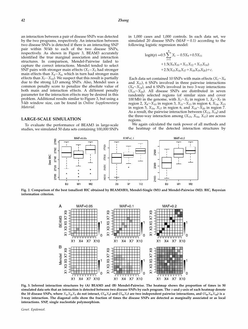
an interaction between a pair of disease SNPs was detectedby the two programs, respectively. An interaction betweentwo disease SNPs is detected if there is an interacting SNPpair within 50 kb to each of the two disease SNPs,respectively. As shown in Figure 3, BEAM3 accuratelyidentified the true marginal association and interactionstructures. In comparison, Mendel-Pairwise failed tocapture the correct interactions. Mendel tended to selectSNP pairs with stronger main effects (X1�X3 had strongermain effects than X4�X6, which in turn had stronger maineffects than X7�X10). We suspect that this result is partiallydue to the strong LD among SNPs. Also, Mendel uses acommon penalty score to penalize the absolute value ofboth main and interaction effects. A different penaltyparameter for the interaction effects may be desired in thisproblem. Additional results similar to Figure 3, but using a5-kb window size, can be found in Online SupplementaryMaterial.

LARGE-SCALE SIMULATION

To evaluate the performance of BEAM3 in large-scalestudies, we simulated 50 data sets containing 100,000 SNPs

in 1,000 cases and 1,000 controls. In each data set, wesimulated 20 disease SNPs (MAF 5 0.1) according to thefollowing logistic regression model:

logitðpÞ ¼0:5X8

i¼1

Xi � 0:5X910:5X11

11:5ðX9X101X11X121X13X14Þ

12:5ðX15X16X171X18X19X20Þ1c:

Each data set contained 10 SNPs with main effects (X1�X9

and X11), 6 SNPs involved in three pairwise interactions(X9�X14), and 6 SNPs involved in two 3-way interactions(X15�X20). All disease SNPs are distributed in sevenrandomly selected regions (of similar sizes and cover100 Mb) in the genome, with X1�X3 in region 1, X4�X7 inregion 2, X8�X10 in region 3, X11�X13 in region 4, X14, X15

in region 5, X16, X17 in region 6, and X18�X20 in region 7.As a result, the pairwise interaction between (X13, X14) andthe three-way interaction among (X15, X16, X17) are acrossregions.

We again calculated the rank power of all methods andthe heatmap of the detected interaction structures by

Fig. 2. Comparison of the best (smallest) BIC obtained by BEAM3(B3), Mendel-Single (M1) and Mendel-Pairwise (M2). BIC, Bayesianinformation criterion.

Fig. 3. Inferred interaction structures by (A) BEAM3 and (B) Mendel-Pairwise. The heatmap shows the proportion of times in 50simulated data sets that an interaction is detected between two disease SNPs by each program. The x-and y-axis of each heatmap denote

the 10 disease SNPs, where X1,X2,X3 do not interact, (X4,X5) and (X6,X7) are two independent pairwise interactions, and (X8,X9,X10) is a

3-way interaction. The diagonal cells show the fraction of times the disease SNPs are detected as marginally associated or as local

interactions. SNP, single nucleotide polymorphism.

42 Zhang

Genet. Epidemiol.

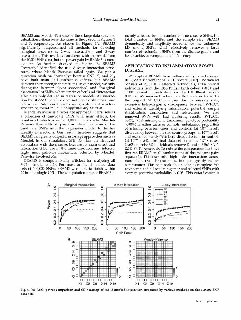
BEAM3 and Mendel-Pairwise on these large data sets. Thecalculation criteria were the same as those used in Figures 1and 3, respectively. As shown in Figure 4A, BEAM3significantly outperformed all methods for detectingmarginal associations, 2-way interactions, and 3-wayinteractions. This result is consistent with the result fromthe 10,000 SNP data, but the power gain by BEAM3 is moreevident. As further observed in Figure 4B, BEAM3‘‘correctly’’ identified the true disease interaction struc-tures, where Mendel-Pairwise failed again. We put aquotation mark on ‘‘correctly’’ because SNP X9 and X11

have both main and interaction effects, but BEAM3detected them through interactions. In our model, we onlydistinguish between ‘‘joint association’’ and ‘‘marginalassociation’’ of SNPs, where ‘‘main effect’’ and ‘‘interactioneffect’’ are only defined in regression models. An interac-tion by BEAM3 therefore does not necessarily mean pureinteraction. Additional results using a different windowsize can be found in Online Supplementary Material.

Mendel-Pairwise is a two-stage approach. It first selectsa collection of candidate SNPs with main effects, thenumber of which is set at 1,000 in this study. Mendel-Pairwise then adds all pairwise interaction terms of thecandidate SNPs into the regression model to furtheridentify interactions. Our result therefore suggests thatBEAM3 can greatly outperform 2-stage approaches such asMendel. In our simulation, SNP X11 has the strongestassociation with the disease, because its main effect andinteraction effect are in the same direction, and interest-ingly, most pairwise interactions selected by Mendel-Pairwise involved X11.

BEAM3 is computationally efficient for analyzing allSNPs simultaneously. For most of the simulated datasets of 100,000 SNPs, BEAM3 were able to finish within20 hr on a single CPU. The computation time of BEAM3 is

mainly affected by the number of true disease SNPs, thetotal number of SNPs, and the sample size. BEAM3dynamically and implicitly accounts for the unknownLD among SNPs, which effectively removes a largenumber of redundant SNPs from the disease graph, andhence achieves computational efficiency.

APPLICATION TO INFLAMMATORY BOWELDISEASE

We applied BEAM3 to an inflammatory bowel disease(IBD) data set from the WTCCC project [2007]. The data setconsists of 2,005 IBD affected individuals, 1,504 normalindividuals from the 1958 British Birth cohort (58C), and1,500 normal individuals from the UK Blood Service(UKBS). We removed individuals that were excluded bythe original WTCCC analysis due to missing data,excessive heterozygosity, discrepancy between WTCCCand external identifying information, potential samplestratification, duplication and relatedness. We alsoremoved SNPs with bad clustering results (WTCCC,2007), 42% missing data (maximum genotype probabilityo90%) in either cases or controls, unbalanced proportionof missing between cases and controls (at 10�3 level),discrepancy between the two control groups (at 10�6 level),and excessive Hardy-Weinberg disequilibrium in controls(at 10�6 level). The final data set contained 1,748 cases,2,962 controls (6% individuals removed), and 403,561 SNPs(20% SNPs removed). To reduce the computation load, wefirst ran BEAM3 on all combinations of chromosome pairsseparately. This may miss high-order interactions acrossmore than two chromosomes, but can greatly reducecomputation. This step took about 12 hr to complete. Wenext combined all results together and selected SNPs withaverage posterior probability 40.05. This cufoff choice is

Fig. 4. (A) Rank power comparison and (B) heatmap of the identified interaction structures by various methods on the 100,000 SNP

data sets.

43Novel Bayesian Graphical Model

Genet. Epidemiol.

arbitrary. We then included neighboring SNPs within 50 kbto the selected SNPs. The filtered data set contained 3,809SNPs, a 100 times reduction from the original data set. Wereran BEAM3 on the filtered data set to obtain the finalposterior distribution of SNP association and interaction.

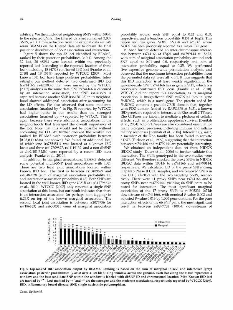
Figure 5 shows the top 32 loci identified by BEAM3,ranked by their posterior probabilities (Z0.1). Among the32 loci, 20 (63%) were located within the previouslyreported loci (according to the reported location of theseloci), including 15 (47%) confirmed IBD loci [Franke et al.,2010] and 18 (56%) reported by WTCCC [2007]. Mostknown IBD loci have large posterior probabilities. Inter-estingly, our method detected two confirmed IBD loci(rs744166, rs4263839) that were missed by the WTCCC[2007] analysis in the same data. SNP rs744166 is capturedby an interaction association, and SNP rs4263839 iscaptured because another SNP (rs6478108) in its neighbor-hood showed additional association after accounting forthe LD effects. We also observed that some moderateassociations (marked by ^ in Fig. 5) reported by WTCCChad higher ranks in our results than the strongestassociations (marked by 1) reported by WTCCC. This isagain because there were additional associations in theneighborhoods that leveraged the overall importance ofthe loci. Note that this would not be possible withoutaccounting for LD. We further checked the weaker lociranked by BEAM3 with posterior probability between[0.05,0.1) (data not shown). We found 20 additional loci,of which one (rs7554511) was located at a known IBDlocus and three (rs17309827, rs11119132, and a non-dbSNPat chr2:101.7 Mb) were reported by a recent IBD metaanalysis [Franke et al., 2010].

In addition to marginal associations, BEAM3 detectedsome potential multi-SNP joint associations with IBD.There are two local joint associations located withinknown IBD loci. The first is between rs10489629 andrs10489628 (sum of marginal association probability 1.0and interaction association probability 0.43). Both SNPs arelocated in the well-known IBD gene IL23R at 1p31 [Frankeet al., 2010]. WTCCC [2007] only reported a single SNPassociation at this locus, but our result indicates that thereis an interaction association (or perhaps joint-tagging) inIL23R on top of the known marginal association. Thesecond local joint association is between rs2076756 (orrs7186163) and rs6500315 (sum of marginal association

probability around each SNP equal to 0.62 and 0.03,respectively, and interaction probability 0.45) at 16q12. Thisregion includes genes NDK1, SNX20 and NOD2, whereNOD2 has been previously reported as a major IBD gene.

BEAM3 further detected an inter-chromosome interac-tion between rs744166 at 17q21 and rs4799144 at 18q23,with sum of marginal association probability around eachSNP equal to 0.01 and 0.0, respectively, and sum ofinteraction probability equal to 0.25. We performedfive expensive genome-wide permutation analysis, andobserved that the maximum interaction probabilities fromthe permuted data set were all o0.1. It thus suggests thatthis IBD interaction is at least weakly significant in thegenome-scale. SNP rs744166 lies in gene STAT3, which is apreviously confirmed IBD locus [Franke et al., 2010].WTCCC did not report this association, as its marginalassociation is insignificant. SNP rs4799144 lies in genePARD6G, which is a novel gene. The protein coded byPARD6G contains a pseudo-CRIB domain that, togetherwith PDZ domain (coded by RAPGEF6 at 5q31, a knownIBD gene), are required to interact with Rho small GTPases.Rho GTPases are known to mediate a plethora of cellulareffects, such as proliferation, apoptosis/survival [Benitahet al., 2004]. Rho GTPases are also considered essential formany biological processes, including immune and inflam-matory responses [Benitah et al., 2004]. Interestingly, Rac1,a member of the Rho family, has been found to activateSTAT3 [Turkson et al., 1999], suggesting that the interactionbetween rs744166 and rs4799144 are potentially interesting.

We obtained an independent data set from NIDDKIBDGC study [Duerr et al., 2006] to further validate thisinteraction. The SNPs genotyped in the two studies weredifferent. We therefore checked the proxy SNPs in NIDDKIBDGC data within 100 kb to rs744166 and rs4799144,respectively. We calculated LD of the proxy SNPs usingHapMap Phase II CEU samples, and we removed SNPs inlow LD (|r|o0.2) with the two targeting SNPs, respec-tively. There were 11 proxy SNPs near rs744166 and 6proxy SNPs near rs4799144, yielding 66 SNP pairs to betested for interaction. The most significant marginalassociation of the 17 proxy SNPs is rs1905339 (67 kbdownstream of rs744166), with nominal P-value 0.002 andadjusted P-value 0.016 by 1,000 permutations. For the pureinteraction effects of the 66 SNP pairs, the most significantresult is between rs9897702 (100 kb downstream of

Fig. 5. Top-ranked IBD association output by BEAM3. Ranking is based on the sum of marginal (black) and interactive (gray)association posterior probabilities (y-axis) over a 100-kb sliding window across the genome. Each bar along the x-axis represents a

window, and the best candidate SNP within the window is labeled with dbSNP ID and chromosomal location (Mb). Known IBD loci

are marked by ‘%.’ Loci marked by ‘1’ and ‘^’ are the strongest and the moderate associations, respectively, reported by WTCCC [2007].

IBD, inflammatory bowel disease; SNP, single nucleotide polymorphism.

44 Zhang

Genet. Epidemiol.

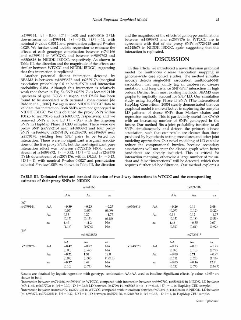
rs4799144, |r| 5 0.30, |D0| 5 0.63) and rs6506816 (17 kbdownstream of rs4799144, |r| 5 0.48, |D0| 5 1), withnominal P-value 0.0012 and permutation adjusted P-value0.025. We further used logistic regression to estimate theeffects of each genotype combination between rs744166and rs4799144 in WTCCC, and between rs9897702 andrs6506816 in NIDDK IBDGC, respectively. As shown inTable III, the direction and the magnitude of the effects aresimilar between WTCCC and NIDDK IBDGC, suggestingthat this interaction is replicated.

Another potential distant interaction detected byBEAM3 is between rs16893872 and rs2579176 (marginalassociation probability 0.0 at both SNPs and interactionprobability 0.08). Although this interaction is relativelyweak (not shown in Fig. 5), SNP rs2579176 is located 21 kbupstream of gene DLG5 at 10q22, and DLG5 has beenfound to be associated with perianal Crohn disease [deRidder et al., 2007]. We again used NIDDK IBDGC data tovalidate this interaction. Both SNPs were not genotyped inNIDDK IBDGC. We thus obtained the proxy SNPs within100 kb to rs2579176 and rs16893872, respectively, and weremoved SNPs in low LD (|r|o0.2) with the targetingSNPs in HapMap Phase II CEU samples. There were oneproxy SNP (rs7729215) near rs16893872 and four proxySNPs (rs1866437, rs2579159, rs1248678, rs1248688) nearrs2579176, yielding four SNP pairs to be tested forinteraction. There were no significant marginal associa-tions of the five proxy SNPs, but the most significant pureinteraction effect was between rs7729215 (45 kb down-stream of rs16893872, |r|5 0.32, |D0|5 1) and rs1248678(78 kb downstream of rs2579176, within DLG5, |r|5 0.43,|D0|5 1), with nominal P-value 0.0027 and permutationadjusted P-value 0.005. As shown in Table III, the direction

and the magnitude of the effects of genotype combinationsbetween rs16893872 and rs2579176 in WTCCC are inagreement with that of the proxy SNPs rs7729215 andrs1248678 in NIDDK IBDGC, again suggesting that thisinteraction is replicated.

DISCUSSION

In this article, we introduced a novel Bayesian graphicalmodel for multilocus disease association mapping ingenome-wide case control studies. The method simulta-neously detects single-SNP association, multilocal-SNPassociation that may jointly tag an unobserved diseasemutation, and long distance SNP-SNP interaction in highorders. Distinct from most existing methods, BEAM3 usesgraphs to implicitly account for SNP LD. Our simulationstudy using HapMap Phase II SNPs [The InternationalHapMap Consortium, 2005] clearly demonstrated that ourgraphical model is more effective in capturing the complexLD patterns of dense SNPs than Markov chains andregression methods. This is particularly useful for GWASwith an increasing number of SNPs genotyped in thefuture. Our method fits a joint probability function to allSNPs simultaneously and detects the primary diseaseassociation, such that our results are cleaner than thoseproduced by hypothesis testing procedures and other jointmodeling approaches. Our novel modeling of LD can alsoreduce the computational burden, because secondaryassociations will not enter the disease graph when bettercandidates are already included. This is critical forinteraction mapping, otherwise a large number of redun-dant and false ‘‘interactions’’ will be detected, which thenrequires further ad hoc filtration. Our method explores a

TABLE III. Estimated effect and standard deviation of two 2-way interactions in WTCCC and the correspondingestimates of their proxy SNPs in NIDDK

rs744166 rs9897702

AA Aa aa AA Aa aa

(A)a

rs4799144 AA �0.39 �0.23 �0.27 rs6506816 AA �0.26 0.16 0.49

(0.05) (0.07) (0.09) (0.07) (0.12) (0.22)Aa 0.33 0.22 �1.77 Aa 0.19 0.12 �1.07

(0.17) (0.15) (0.48) (0.15) (0.18) (0.51)aa 1.49 �11.2 NA aa 1.43 �0.55 0.67

(1.16) (197.0) NA (0.52) (0.61) (0.92)(B)b

rs16893872 rs7729215

AA Aa aa AA Aa aars2579176 AA �0.42 �0.27 NA rs1248678 AA �0.13 �0.31 �1.25

(0.05) (0.47) NA (0.07) (0.18) (0.79)Aa �0.21 1.52 12.0 Aa �0.08 0.71 �0.97

(0.07) (0.37) (197.0) (0.11) (0.23) (1.16)aa �0.37 0.42 NA aa �0.05 �0.16 12.7

(0.10) (0.71) NA (0.21) (0.77) (324.7)

Results are obtained by logistic regression with genotype combination AA/AA used as baseline. Significant effects (p-value o0.05) areshown in bold.aInteraction between (rs744166, rs4799144) in WTCCC, compared with interaction between (rs9897702, rs6506816) in NIDDK. LD between(rs744166, rs9897702) is |r|5 0.30, |D0|5 0.63; LD between (rs4799144, rs6506816) is |r|5 0.48, |D0|5 1, in HapMap CEU sample.bInteraction between (rs16893872, rs2579176) in WTCCC, compared with interaction between (rs7729215, rs1248678) in NIDDK. LD between(rs16893872, rs7729215) is |r|5 0.32, |D0|5 1; LD between (rs2579176, rs1248678) is |r|5 0.43, |D0|5 1, in HapMap CEU sample.

45Novel Bayesian Graphical Model

Genet. Epidemiol.

variety of combinations of SNPs and interaction structuresvia regularized probability functions, by which we meanthat all model parameters are treated as random in aBayesian framework, and we analytically integrate out allnuisance parameters, such that the complexity of variousinteraction structures are automatically standardized bythe normalizing constants of their corresponding distribu-tions. BEAM3 therefore automatically strikes a balancebetween the power of disease mapping and the modelcomplexity. As demonstrated by simulation, BEAM3outperformed all other tested methods and identified themost accurate disease models.

We successfully applied BEAM3 to WTCCC IBD data[WTCCC, 2007], which consists of 4,720 individuals and401,473 SNPs after quality control. Our method iscomputationally affordable to analyze this huge data set.Not only we detected all loci that were previously reportedin this data, but also we recovered two missed IBD loci. Wefurther detected a few novel IBD loci and interactionassociations. In particular, the interaction between genesSTAT3 (a known IBD gene but missed by WTCCC) andPARD6G (a novel locus) has biological connections and isfurther validated by the NIDDK IBDGC data set [Duerret al., 2006]. Another potential interaction is between DLG5and an intergenic region at 5p14. Again, DLG5 is a knownIBD gene missed by WTCCC [2007], and we validated thisinteraction in the NIDDK IBDGC data set.

The WTCCC IBD data set has been analyzed by others.Liu et al. [2011] reported two interactions in the WTCCCIBD data. The first interaction is between rs7522462 andrs11945978, which has a combined P-value (main1inter-action effect) 0.039 after multiple comparison adjustment.This is done using expanded controls, i.e., includingpatients from other diseases as controls. Using ourmethod, however, we found the two SNPs are more likelyto affect the disease risk independently. Despite that weonly used the normal people as controls, the discrepancybetween the two studies may be attributable to thedifferent models. Liu et al. [2011] treated the SNP effectsas unknown but constant parameters, while we treatedgenotype frequencies as random variables following aDirichlet distribution. Furthermore, our model assumes thatthe frequencies of genotype combinations are all differentbetween cases and controls under the alternative hypothesis.The two SNPs, however, only showed frequency differencein two of nine genotype combinations, where the other 7combinations confirmed almost perfectly to independence.As a result, our marginal association model has largerlikelihood than our interaction model, because the formerhas less complexity and variability. A larger sample sizewould resolve this discrepancy. The second interactionreported by Liu et al. [2011] is between rs153423 andrs748855, with adjusted P-value 0.146 using expandedcontrols. When testing the two SNPs alone, the interactionis indeed identifiable by our method. When testing togetherwith their neighboring SNPs, very interestingly, the interac-tion disappeared. SNP rs748855 lies in NOD2, a well-knownIBD gene. There are several other SNPs in NOD2 with muchstronger associations with IBD. The approach taken by Liuet al. [2011] ignores the dependence between SNPs. Theinteraction is thus likely created by LD effects. Thisinteraction in fact was not replicated by the proxy SNPs[Liu et al., 2011] in NIDDK IBDGC.

Our method can be improved in several aspects. Mostassociation signals in GWAS are weak, particularly for

multi-SNP associations. Our current model is still restrictivein that it assumes all allele combination frequencies in aSNP set are all different between cases and controls. Thisassumption could be relaxed by allowing subset frequencydifferences using a mixture model, which will thenimprove the power of detecting subtle interactions. It isalso desirable to include expert knowledge of disease lociand potential interactions between genes involved the samebiological processes as a prior in our model. This isstraightforward to implement in a Bayesian framework.In addition, the current model does not include covariates,such as environment factors and population structures. Onepossible way to incorporate covariates is to replace all theprobability functions in our model by conditional prob-ability functions giving the covariates. Finally, the compu-tation speed of our method could be further improved. Onesolution is to utilize parallel computing infrastructures tosplit the task into smaller pieces and run each piece inparallel. Although we applied a similar idea in analyzingthe WTCCC IBD data, a real parallel implementation isneeded for analyzing larger data sets with hundreds ofthousands individuals and many millions of SNPs.

ACKNOWLEDGMENTS

Y.Z. is supported by NIH grant R01-HG004718. The dataof the WTCCC IBD study is obtained from the WellcomeTrust Case-Control Consortium. The data of the NIDDKIBDGC study (phs000130.v1.p1) is obtained from dbGaP.All the chromosomal positions are in NCBI build 35coordinates.

REFERENCESBenitah SA, Valern PF, van Aelst L, Marshall CJ, Lacal JC. 2004. Rho

GTPases in human cancer: an unresolved link to upstream and

downstream transcriptional regulation. Biochim Biophys Acta

1705:121–132.

Cirulli ET, Goldstein DB. 2010. Uncovering the roles of rare variants in

common disease through whole-genome sequencing. Nat RevGenet 11:415–425.

Cordell HJ. 2009. Detecting gene-gene interactions that underline

human diseases. Nat Genet 10:392–404.

de Bakker PI, Yelensky R, Pe’er I, Gabriel SB, Daly MJ, Altshuler D.

2005. Efficiency and power in genetic association studies. Nat

Genet 37:1217–1223.

de Ridder L, Weersma RK, Dijkstra G, van der Steege G, Benninga

MA, Nolte IM, Taminiau JA, Hommes DW, Stokkers PC. 2007.

Genetic susceptibility has a more important role in pediatric-onset

Crohn’s disease than in adult-onset Crohn’s disease. Inflamm

Bowel Dis 13:1083–1092.

DiCiccio TJ, Kass RE, Raftery A, Wasserman L. 1997. Computing Bayes

factors by combining simulation and asymptotic approximations.

J Am Stat Assoc 92:902–915.

Duerr RH, Taylor KD, Brant SR, Rioux JD, Silverberg MS, et al. 2006.

A genome-wide association study identifies IL23R as an inflam-

matory bowel disease gene. Science 314:1461–1463.

Franke A, McGovern DP, Barrett JC, Wang K, Radford-Smith GL,

Ahmad T, Lees CW, Balschun T, Lee J, Roberts R, Anderson CA,Bis JC, Bumpstead S, Ellinghaus D, Festen EM, Georges M, Green

T, Haritunians T, Jostins L, Latiano A, Mathew CG, Montgomery

GW, Prescott NJ, Raychaudhuri S, Rotter JI, Schumm P, Sharma Y,

Simms LA, Taylor KD, Whiteman D, Wijmenga C, Baldassano RN,

Barclay M, Bayless TM, Brand S, Byning C, Cohen A, Colombel JF,

Cottone M, Stronati L, Denson T, De Vos M, D’Inca R, Dubinsky M,

Edwards C, Florin T, Franchimont D, Gearry R, Glas J, Van

46 Zhang

Genet. Epidemiol.

Gossum A, Guthery SL, Halfvarson J, Verspaget HW, Hugot JP,

Karban A, Laukens D, Lawrance I, Lemann M, Levine A, Libioulle

C, Louis E, Mowat C, Newman W, Panzs J, Phillips A, Proctor DD,

Regueiro M, Russell R, Rutgeerts P, Sanderson J, Sans M, Seibold F,

Steinhart AH, Stokkers PC, Torkvist L, Kullak-Ublick G, Wilson D,

Walters T, Targan SR, Brant SR, Rioux JD, D’Amato M, Weersma

RK, Kugathasan S, Griffiths AM, Mansfield JC, Vermeire S, Duerr

RH, Silverberg MS, Satsangi J, Schreiber S, Cho JH, Annese V,

Hakonarson H, Daly MJ, Parkes M. 2010. Genome-wide meta-

analysis increases to 71 the number of confirmed Crohn’s disease

susceptibility loci. Nat Genet 42:1118–1125.

Kuno S, Taniguchi A, Saito A, Tsuchida-Otsuka S, Kamatani N. 2004.

Comparison between various strategies for the disease-gene

mapping using linkage disequilibrium analyses: studies onadenine phosphoribosyltransferase deficiency used as an example.

J Hum Genet 49:463–473.

Liu Y, Xu H, Chen S, Chen X, Zhang Z, Zhu Z, Qin X, Hu L, Zhu J,

Zhao GP, Kong X. 2011. Genome-wide interaction-based associa-

tion analysis identified multiple new susceptibility Loci for

common diseases. PLoS Genet 7:e1001338.

Marchini J, Donnelly P, Cardon LR. 2005. Genome-wide strategies for

detecting multiple loci that influence complex diseases. Nat Genet

37:413–417.

Metzker ML. 2010. Sequencing technologies—the next generation. Nat

Rev Genet 11:31–46.

Moore JH, Williams SM. 2002. New strategies for identifying gene-

gene interactions in hypertension. Ann Med 34:88–95.

Pitman J, Yor M. 1997. The two-parameter Poisson-Dirichlet distribu-

tion derived from a stable subordinator. Ann Prob 25:855–900.

Schwartz DF, Ziegler A, Ksnig IR. 2008. Beyond the results of genome-

wide association studies. Genet Epidemiol 32:671.

The International HapMap Consortium. 2005. A haplotype map of the

human genome. Nature 437:1299–1320.

The Wellcome Trust Case Control Consortium. [21]2007. Genome-wide

association study of 14,000 cases of seven common diseases and

3,000 shared controls. Nature 447:661–678.

Tibshirani R. 1996. Regression shrinkage and selection via the lasso. J R

Stat Soc B 58:267–288.

Turkson J, Bowman T, Adnane J, Zhang Y, Djeu JY, Sekharam M, Frank

DA, Holzman LB, Wu J, Sebti S, Jove R. 1999. Requirement for

Ras/Rac1-mediated p38 and c-Jun N-terminal kinase signaling in

Stat3 transcriptional activity induced by the Src oncoprotein. Mol

Cell Biol 19:7519–7528.Wan X, Yang C, Yang Q, Xue H, Fan X, Tang NL, Yu W. 2010.

BOOST: A fast approach to detecting gene-gene interactions

in genome-wide case-control studies. Am J Hum Genet 87:

325–340.

Wu TT, Chen YF, Hastie T, Sobel E, Lange K. 2009. Genome-wide

association analysis by lasso penalized logistic regression. Bioin-

formatics 25:714–721.

Zhang Y, Liu JS. 2007. Bayesian inference of epistatic interactions in

case-control studies. Nat Genet 39:1167–1173.

Zhang K, Calabrese P, Nordborg M, Sun F. 2002. Haplotype structure

and its applications to association studies: power and study

designs. Am J Hum Genet 71:1386–1394.

Zhang Y, Zhang J, Liu JS. 2011. Block-based Bayesian epistasis

association mapping with application to WTCCC Type 1 diabetes

data. Ann Appl Stat 5:2052–2077.

47Novel Bayesian Graphical Model

Genet. Epidemiol.