Received: 17 January 2020 Revised: 15 September 2020 Accepted: 5 November 2020

DOI: 10.1002/nav.21966

R E S E A R C H A R T I C L E

A novel approach for modeling order picking paths

Sabahattin G. Ozden1 Alice E. Smith2 Kevin R. Gue3

1Information Sciences and Technology, Penn State

Abington, Abington, Pennsylvania, USA2Department of Industrial and Systems

Engineering, Auburn University, Auburn,

Alabama, USA3Department Industrial Engineering, University of

Louisville, Louisville, KY, USA

CorrespondenceS. G. Ozden, Information Sciences and Technology,

Penn State Abington, Abington, PA 19001, USA.

Email: gokhan@psu.edu

Funding informationDivision of Civil, Mechanical and Manufacturing

Innovation, Grant/Award Number: 1200567.

National Science Foundation, Grant/Award

Number: CMMI-1200567.

AbstractWe introduce the visibility graph as an alternative way to estimate the length of aroute traveled by order pickers in a warehouse. Heretofore it has been assumed thatworkers travel along a network of travel paths corresponding to centers of aisles,including along the right angles formed where picking aisles join cross aisles. Avisibility graph forms travel paths that correspond to more direct and, we believe,more appropriate “travel by sight.” We compare distance estimations of the visibilitygraph and the aisle-centers method analytically for a common traditional warehousedesign. We conduct a range of computational experiments for both traditional andfishbone warehouse layouts to assess the impact of this change in distance metric.Distance estimations using aisle-centers calculates a length of a picking tour on aver-age 10–20% longer compared to distance estimations based on the visibility graph.The visibility graph metric also has implications for warehouse design: when com-paring three traditional layouts, the distance model using a visibility graph resultedin choosing a different best layout in 13.3% of the cases.

KEYWORDS

computational geometry, routing, shortest path problem, visibility graph, warehousedesign

1 INTRODUCTION

An important part of warehouse modeling is the task ofdetermining the distance between two points. Virtually everywarehousing paper in the literature uses the rectilinear orManhattan metric to estimate the distance between two points.However, in practice often workers “cut corners” and do notmake turns at exact right angles (see Figure 1). The effectsof this imprecision when modeling depend on the size ofthe warehouse, the width of aisles, the number of cornersa worker could cut, and most importantly, the question oneseeks to answer with the model. As we will show, the existingdistance metric almost certainly over-estimates the distancetraveled by workers, and therefore labor costs are most likelyover-estimated and throughput rates are under-estimated.However, if the question addresses different operating poli-cies within the same layout the results are “relatively correct,”or at least mostly so. However, for different warehouse lay-outs this relative effect may not hold. In summary, the choiceof distance metric can affect which layout design is most suit-able and if the visibility graph models worker travel with

more fidelity, using it during warehouse design will result intruly superior layouts. The purpose of this paper is to explainthis effect and to offer an alternative distance metric, whichwe argue is more appropriate for modeling travel paths ofworkers in a warehouse especially in manual order pickingoperations. In automated environments, the effects are muchreduced such as in the case where forklifts are used where theuse of predetermined lanes reduces the possibility of cuttingcorners. Automated Guided Vehicles generally also followa fixed path, which is well represented by the aisle-centersmetric.

In their model of a warehouse, Gue and Meller (2009)assumed a network in which nodes represent picking points(e.g., in front of pallet locations), the intersections of crossaisles and picking aisles, and the pick up and deposit point(P&D). Without explicitly saying so, they defined a graphnetwork using the “aisle-centers method” in which the pathbetween points in different picking aisles or between a picklocation and the P&D point passes through the single pointof intersection between the picking aisle(s) and the cross aisle(see Figure 2). This assumption has a limited effect on their

Naval Res Logistics 2020;1–14 wileyonlinelibrary.com/journal/nav © 2020 Wiley Periodicals LLC 1

2 OZDEN ET AL.

s

d

FIGURE 1 Example of a shortest path using a rectilinear distance (short

dashes) versus a path that cuts the corners (long dashes) [Colour figure can

be viewed at wileyonlinelibrary.com]

FIGURE 2 A graph network using the aisle-centers method defined by

Gue and Meller (2009)

problem because they are only interested in paths betweenlocations and the P&D point, and the paths generated by theirmodels are similar to those that one would suppose beingtaken by a typical worker.

One of the most important statistics in an order pickingwarehouse is the (average) pick tour length. Every favorableangle has a corresponding unfavorable angle that poorly rep-resents what might be expected of ordinary worker travelpatterns. By any reasonable estimate of worker behavior,using the network model of Gue and Meller (2009) overesti-mates the distance of tours that require turns of greater than90 degrees (see Figure 3).

We propose the alternative approach of using visibilitygraph based distances between points in a warehouse to repre-sent reasonable levels of corner cutting that one would expectof productive order pickers and compare them with the dis-tances based on aisle-centers. The visibility graph is a specialgraph whose nodes are the vertices of obstacles (or pointsof attraction) and whose edges are pairs of mutually visiblenodes. Figure 3b shows an example of a pick path using a vis-ibility graph, where obstacles are the storage locations (racksor pallets). These proposed paths also serve as a lower boundon travel distances because no shorter path exists withoutpassing through obstacles. However, the example in Figure 3bhas its own issue: because storage locations are themselvesobstacles, paths intersect storage racks along their perimeters.To address this difficulty, we create a buffer distance aroundstorage locations and present the effects of the size of thebuffer distance in Section 3.

Pohl et al. (2009b) used the aisle-centers metric to comparea fishbone layout to a traditional layout for dual commandoperations and found that the fishbone layout can reducetravel distance by 10–15%. Çelik and Süral (2014) also usedthe aisle-centers metric to compare a fishbone layout to atraditional layout for general order picking operations. Theyfound that the fishbone layout can perform up to 30% worsethan an equivalent traditional layout as the number of picksincreases. Hall (1993) developed distance approximationsfor a one block warehouse by using the aisle-centers met-ric and compared different picking strategies for routing amanual order picker. Petersen (1999), Dijkstra and Rood-bergen (2017), and Altarazi and Ammouri (2018) used theaisle-centers metric to compare various storage policies androuting heuristics simultaneously. Roodbergen et al. (2008)used the aisle-centers metric to optimize a traditional layoutby finding the optimal number of pick and cross aisles and thelength of a pick aisle, excluding the width of the cross aisles.Theys et al. (2010) used the aisle-centers metric to comparewell known routing heuristics such as S-shape to dedicatedtraveling salesman problem (TSP) heuristics and found up to47% average savings in route distance. Çelik and Süral (2019)considered the order picking problem as a special case of theSteiner TSP and proposed a routing heuristic that uses theSteiner TSP’s graph theoretic properties. Like all the previouspapers that used the Steiner TSP for order picking problemssuch as Ratliff and Rosenthal (1983) and Roodbergen and DeKoster (2001b), their distance model was based on the aislecenters-method. Our focus is to model and use an alterna-tive metric for estimating distances of order picking tours andto determine if these distances, which we believe are morereasonable estimates of real worker behavior, make a differ-ence in warehouse design, such as investigated by Roodbergenand De Koster (2001a), Roodbergen and Vis (2006), and Gueand Meller (2009). Our experiments address the followingquestions:

• By how much does expected travel distance differ betweenthe two distance estimation metrics for a particular layout?

• Using a visibility graph, does the best layout design changefrom the best design assessed with aisle-centers whencomparing traditional layouts A, B, and C (Figure 4)?

• How does the size of the warehouse, the number of picks,and demand skewness affect the difference between thetwo distance estimation metrics?

The aim of using visibility graphs to model travel distancesis not to find shorter paths than those of aisle-centers, butrather to model more closely the distances that typical workerswould travel. We postulate that paths produced by the visibil-ity graph with suitable buffers are closer to the actual distancetraveled, however validation of this assertion must be left toan empirical study of real worker behavior.

The rest of this paper is organized as follows. In the nextsection, the literature review related to the shortest pathproblem is presented. In Section 3, the model to calculate the

OZDEN ET AL. 3

(A) A pick path by following aisle-centers (B) A pick path by using a visibility graph

FIGURE 3 Pick path examples for picking two items from the storage locations shown in bold and returning to the depot (at bottom center) [Colour figure

can be viewed at wileyonlinelibrary.com]

(A) Fishbone Layout (B) Traditional Layout A

(C) Traditional Layout B (D) Traditional Layout C

FIGURE 4 Four warehouse layouts used throughout this paper (dimensions of the warehouse might change depending on the number of SKUs based on the

experiment, i.e., number of aisles and storage locations are not constant)

average distance of a tour for a given warehouse layout and setof pick lists is developed by using the visibility graph distancemetric. In Section 4, we address the questions described inSection 1 with three experiments. Conclusions are presentedin Section 5.

2 THE SHORTEST PATH PROBLEM

The shortest path problem (SPP) seeks a path from a spe-cific origin to a specific destination in a network such that thetotal cost is minimized. The SPP has widespread applicationsincluding vehicle routing in transportation systems (Zhan &Noon, 1998), telecommunications (Moy, 1994), VLSI design(Peyer et al., 2009), and path planning in robotics (Soueres& Laumond, 1996). There are well-known algorithms for

solving the SPP, including Dijkstra’s algorithm for solving thesingle source SPP with nonnegative weights (Dijkstra, 1959),the Bellman–Ford–Moore algorithm for solving the singlesource SPP with possible negative weights (Bellman, 1958;Ford, 1956; Moore, 1959), the A* search algorithm for solv-ing the single source SPP using heuristics for fast evaluation(Hart et al., 1968), the Floyd–Warshall algorithm for solvingthe all-pairs SPP (Floyd, 1962), and Johnson’s algorithm forsolving the all-pairs SPP on sparse graphs (Johnson, 1977).The details of these algorithms can be found in Gallo andPallottino (1986). The all-pairs SPP has been also studiedon massively parallel computer architectures using parallelcomputing (Habbal et al., 1994).

The Euclidean shortest path problem (ESPP) seeks theshortest path between two points in Euclidean space thatdoes not intersect any of a given set of obstacles. There exist

4 OZDEN ET AL.

efficient exact algorithms with (n log n) time complexityfor problems in the plane, where n is the number of nodesin the graph (Hershberger & Suri, 1999). In three or moredimensions, the Euclidean shortest path problem is NP-hard(Canny & Reif, 1987). In this paper, we are interested in exactalgorithms that work in two dimensional space with multipleobstacles. Hershberger and Suri (1999) state that there havebeen two fundamentally different approaches to this problem:the visibility graph method and the shortest path map method.

The visibility graph method produces a graph whose nodesare the vertices of the obstacles (or attractions) and whoseedges are pairs of mutually visible nodes. In other words,for any pair of nodes, if the line segment that connects themdoes not pass through an obstacle, an edge is created betweenthem. Once the graph is defined, Dijkstra’s algorithm pro-duces the shortest path between any two nodes. The runtime complexity of this approach is O(n log n+E) for sparsegraphs, where E is the number of edges in the graph (Ghosh &Mount, 1991). However, the visibility graph can have n2 edgesin the worst case; therefore algorithms that depend on the vis-ibility graph will have (n2) worst-case run time to find theshortest path between two points. The algorithm we imple-ment in this paper is naïve in that it compares every pair ofpoints in the set of locations and determines whether a linebetween them intersects any edges of obstacles. All pairs haveto be compared with n edges (a set of obstacles with n verticeshas n edges) which makes the overall time complexity of thealgorithm (n3).

The shortest path map method decomposes the plane intoregions such that all points d in a region have the samesequence of obstacle vertices in their shortest path to s. Thelast obstacle vertex along the shortest s− t path is the root rof the cell containing d. The root r can see all points withinits region. Figure 5 shows an example of the shortest pathmap. Point s reaches d via obstacle vertices v and r. In thisexample, vertex r is the root of the region containing d. Her-shberger’s algorithm computes shortest paths in the presenceof polygonal obstacles in (n log n) time and space, where nis the number of nodes in the graph. For a detailed review ofalgorithms that use the visibility graph method or the shortestpath map method, see Toth et al. (2004).

3 METHODOLOGY

There are seven steps to calculate the average distance of atour for a given warehouse layout and set of pick lists. Steps4 and 5 are the tasks related to the visibility graph method.

Step 1: Create exterior aisles for a given width anddepth of the warehouse. These exterior aisles serveas the boundaries of the rectangle-shapedwarehouse.

Step 2: Create cross aisles using exterior and interiorpoints. An exterior point lies on the boundaries of

s

d

rv

FIGURE 5 A shortest path map with respect to source point s within a

polygonal domain with three obstacles. The heavy dashed path indicates the

shortest s− d path, which reaches d via the root r of its cell. Extension

segments are shown thin and dotted [Colour figure can be viewed at

wileyonlinelibrary.com]

the warehouse (i.e., exterior aisles), and an interiorpoint lies inside the boundaries of the warehouse.Cross aisles divide the warehouse into regions.

Step 3: Create pick aisles, pick locations, and storagelocations for each region. We assume that items onboth sides of a pick aisle may be accessed withnegligible lateral movement. Each region may havedifferent angled pick aisles. Figure 6 illustrates sucha warehouse.

Step 4: Calculate polygons that will be used in thevisibility graph calculation. In this step, we createthe polygons considering a buffer region(Lozano-Pérez & Wesley, 1979). The corners of thepolygons are also included as nodes in the visibilitygraph.

Step 5: Let B be the set of polygons which areconstructed for each storage location including abuffer region of size β. We define the visibilitygraph as G = (V, E), where V is the set of nodescontaining all pick locations and the corners of eachpolygon in B and where E is the set of edgesbetween the nodes that are in line of sight of eachother. Then, the set of edges is defined as:

E ={(n1, n2)|n1, n2 ∈ V with n1 ≠ n2, and⋃

Bj∈BLn1,n2

∩ Bj = ∅}, (1)

where Ln1,n2is the set of points on the line segment

that connect node n1 and n2 and Bj is the set ofpoints in polygon j. If for any polygon j,Ln1,n2

∩ Bj ≠ ∅, the line between node n1 and n2 andpolygon j intersect. If no polygon intersects with theline between node n1 and n2, the nodes are in eachother’s line of sight. Furthermore, let dn1,n2

be theEuclidean distance between nodes n1 and n2, for (n1,n2) ∈ E. Finally, the distance between any nodes inV which are not in line of sight can be obtained byapplying Dijkstra’s algorithm (Dijkstra, 1959).

OZDEN ET AL. 5

Cross AislePolygon/Buffer Area Pick Aisle

P&D Point

Pick Location

Storage Location

Exterior Aisle

FIGURE 6 Representation of a warehouse. This particular fishbone layout has a single P&D point, 67 storage locations, 51 pick locations, 9 pick aisles, 2

cross aisles, and 4 exterior aisles. The lines that represent the aisle-centers are both used for building the warehouse structure (i.e., storage locations and pick

locations) and finding the shortest path distances with the aisle-centers method

Step 6: Once the all-pairs shortest path distances arecalculated and stored in the dist matrix, allocateproducts to storage locations. We use a dedicatedstorage policy to keep the locations of the productsidentical between the two distance metrics sostorage will not affect comparisons. We assign theSKU with the smallest ID number to the storagelocation with the smallest ID number and generate adistance matrix for each order by using the distmatrix. In this way, the relative order and positionof each SKU is maintained in any warehouse layoutdesign, making the pick distances comparisons asfair as possible. This matrix contains the shortestpath distances between the P&D point, or depot,and every storage location to be visited. Finding theshortest tour distance in a warehouse for a pick listis an example of a TSP. In the our experiments, wecalculate optimal travel distances using theConcorde TSP solver (Applegate et al., 2007), butany TSP solver can be used.

Step 7: Calculate the average of all TSP distances.

3.1 Adding a buffer

As mentioned before, it is not practical to assume an orderpicker will cut corners so sharply as to brush up along side ofthe storage infrastructure. Therefore, we devise the concept ofthe buffer which artificially increases the size of the storageobstacles so the path better mimics the way a typical humanwould walk. When the size of the buffer increases, the poly-gons (buffer areas) become larger and visibility decreases.Figure 7 shows an example of a visibility graph for a fishbonelayout with a 2 ft buffer size. Figure 8a,b are two examplesof visibility between pick locations. If the buffer size is 1 ft,then pick location 1 is visible to both pick locations 2 and3. However, visibility between pick locations 1 and 2 is lostwhen the buffer size increases to 2 ft.

It is important to note that the density of the visibility graphdecreases with greater buffer size. For example, when thereis no buffer distance between storage locations and pickerpaths there are 1092 arcs created for the visibility graph in thisexample. The number of arcs for 0.5, 1.0, and 2.0 ft buffer dis-tances are 1046, 1014, and 930, respectively. When the buffersize becomes sufficiently large, the visibility graph becomessimilar to the aisle-centers graph.

3.2 Comparison of visibility graph and aisle-centersmethods

While our approach for the paper is one of practical signif-icance of the differences between the aisle-centers methodand the visibility graph method, a baseline can be estab-lished analytically. In this section, we analyze the differencesbetween the visibility graph and aisle-centers methods usingclosed form expressions. To examine this difference in moredetail analytically we must look at a specific layout design.We do so by choosing a very common design - TraditionalLayout A.

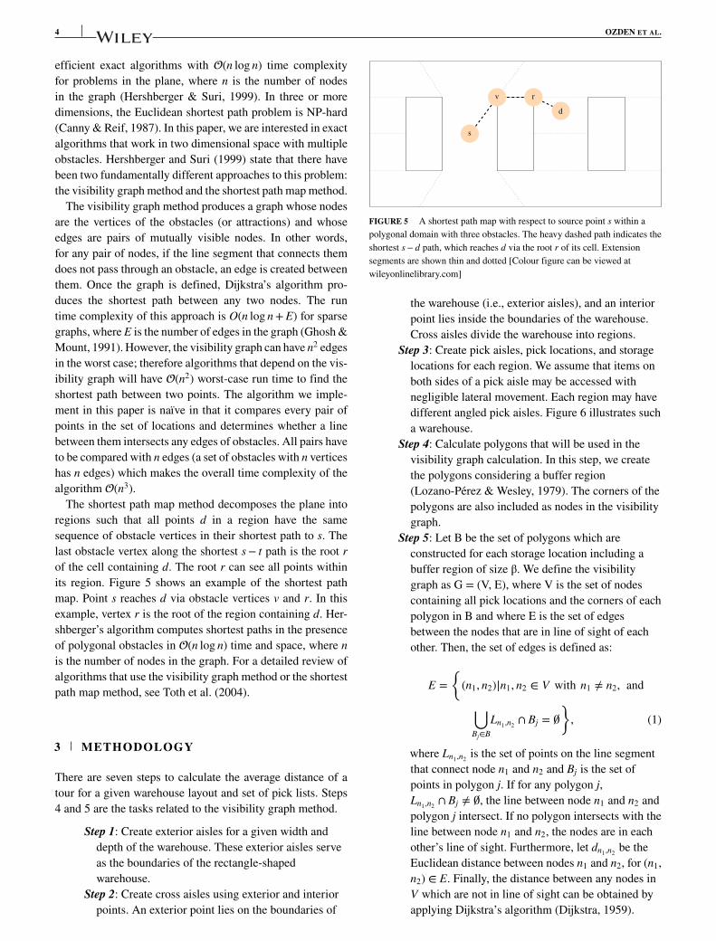
For Traditional Layout A we assume random storage pol-icy which is commonly used in unit-load storage to maxi-mize space utilization. Traditional Layout A, as depicted inFigure 9, has parallel picking aisles that are perpendicularto the front wall, but has no cross aisle. A single depot isoptimally located in the middle of the bottom cross aisleRoodbergen and Vis (2006). Example travel paths betweentwo locations by using aisle-centers and the visibility graphare depicted as solid lines and dashed lines, respectively. Wedo not consider a buffer distance here. The location on the leftis a distance x from the bottom of aisle i and the location onthe right is a distance y from the bottom of aisle j. The lengthof each picking aisle is L and the half width of the cross aisleis v. The warehouse has n picking aisles, where n can be oddor even.

6 OZDEN ET AL.

FIGURE 7 Visibility graph of a fishbone layout with buffer size of 2 ft

(A) (B)

FIGURE 8 Increasing the buffer size decreases the visibility between pick locations

x

L

y

P&D

aislei

aislej

v

vb

c

a

β1

β2β3

β4

FIGURE 9 Traditional layout A [Colour figure can be viewed at wileyonlinelibrary.com]

There is no distance difference between the two methodsif two pick locations are on the same picking aisle (travelbetween distance, TB, will be |x− y|). If two items are on dif-ferent picking aisles, the maximum difference occurs whenaisle i and aisle j are adjacent, i.e., |i− j| = 1. In other cases,the picker travels parallel to the cross aisle which will not per-form the shortcut leveraged by the visibility graph approach.There are n possible ways that i = j, and these incur nocross aisle travel. Therefore, the probability that |i− j| = 0 isn/n2. Similarly, there are 2(n− 1) combinations for the case|i− j| = 1. Therefore, Pr(|i− j| = 1) = 2(n− 1)/n2. In general,

Pr(i − j| = k) = 2(n − k)n2

(2)

Since limn→∞2(n−1)

n2= 0, we can conclude that the number

of aisles, n, for the maximum distance difference is 2. To fullycalculate the expected paths for the visibility graph method,the values of the pick aisle half width, a, the storage loca-tion depth, b, the storage location width c, the cross aisle halfwidth, v, the pick location’s distance to cross aisle in aisle i, x,and the pick location’s distance to the cross aisle in aisle j mustbe included. There are two possible ways of picking: exitingeither from bottom or from top, and both are equally likely

OZDEN ET AL. 7

because of the uniform distribution of picking. The expectedcross aisle travel distance for the visibility graph is

2(n − 1)(a(n − 2) + b(n − 1))3n

(3)

and the expected picking aisle travel distance for the visibilitygraph is

1n

(L3

)+ n − 1

nf1(a,L) (4)

The derivations of (3) and (4) including the definition off 1(a, L) are found in the Appendix. Given (3) and (4), theexpected travel distance between locations for TraditionalLayout A using the visibility method is

E[TBVG] =1n

[L3+ (n − 1)f1(a,L)

]

+ 2(n − 1)(a(n − 2) + b(n − 1))3n

(5)

The expected travel distance between locations for Tradi-tional Layout A using the aisle-centers method (using theequation from Pohl et al. (2009a)) is

E[TBACM] =1n

[L3+ (n − 1)

(23

L + 2v)]

+ 2(a + b)(n2 − 1)3n

(6)

Note that the aisle width term in Pohl et al. (2009a) isreplaced with 2a+ 2b in our version. The expected overesti-mation between the aisle-centers method (using the equationfrom Pohl et al. (2009a) for the expected aisle-centers methoddistance) and visibility graph method can be shown as

E[TBACM] − E[TBVG]E[TBACM]

=

(n − 1)

⎛⎜⎜⎜⎜⎜⎜⎝

16a2√

a2 + L2 − 8L2√

a2 + L2 + 15a2L log(

a√a2+L2+L

)−6a2L log

(√a2+L2+L

a

)− 3a2L tanh−1

(L√

a2+L2

)−16a3 − 8an3 + 40an2 + 24an − 8bn3

+32bn2 + 24bn + 8L + 24v

⎞⎟⎟⎟⎟⎟⎟⎠4(6(n − 1)(an(n + 1) + bn(n + 1) + v) + L(2n − 1))

(7)

If 𝛽1, 𝛽2, 𝛽3, and 𝛽4 are equal to 45◦

the maximum dif-ference between the two distance metrics occurs. This onlyhappens with a single pick location per pick aisle (i.e., L = c)and a = c/2.

Note that an increase in v will increase the distance for theaisle-centers method but does not affect the visibility graphmethod for this type of layout. For any constant values ofx, y, L, a, b, the limv→∞

Min[x+y+2v+2b,(L−x)+(L−a)+2v+2b]Min[

√x2+a2+2b,

√(L−x)2+(L−a)2+2b]

= ∞.

In other words, warehouses with wider cross aisles will havea greater distance difference between the two metrics. Toevaluate visibility graph distances relative to aisle-centers dis-tances, we calculated the expected travel distances betweentwo locations for various values of L,v,b,and n. Our calcula-tions on overestimation by the aisle-centers distance metricfor a variety of warehouse sizes and parameters show a rangeof 0–47%, over a variety of warehouse shapes and sizes (seethe Appendix, Table A1), with the maximum overestimationoccurring with two picking aisles with only a few storagelocations.

4 COMPUTATIONAL RESULTS

To make specific comparisons we devised computationalexperiments with a variety of warehouse layouts, sizes, andpick characterization. For the results that follow, we assumewarehouses between 200 and 1000 pick locations, where alocation is a stopping point that gives access to storage slotson both sides of the aisle. We assume a uniform demandand random storage policy in order not to create “hot zones”

that are visited more often. We assume picking and crossaisles are 12 ft wide and that storage locations are 4× 4 ft. Weuse a 2.5 ft buffer around all obstacles to estimate the pathswith small size pickers such as human pickers with carts.We also used a 3.5 ft buffer around all obstacles to estimatethe paths with large size pickers such as forklifts or auto-mated guided vehicles. These are all reasonable assumptionsin current warehousing (Goetschalckx & Ratliff, 1988).

Picking tours vary between 1 and 30 locations. We usethe order generation method of Çelik and Süral (2014), butinstead of evaluating 100 orders for each pick list size, we varythe number of orders. In general, tours with few picks havea higher variance in travel distance, so we increase the sam-ple size for small pick lists to decrease the variability. Table 1shows the number of orders sampled for each pick list size.The number of orders sampled for each pick list size is suf-ficient to guarantee a relative error of estimating mean traveldistance of at most 1% with a probability 95%.

TABLE 1 Number of orders evaluated foreach pick list size

Pick list size Number of orders

1 10,000

2 5000

3 3333

5 2000

10 1000

30 333

8 OZDEN ET AL.

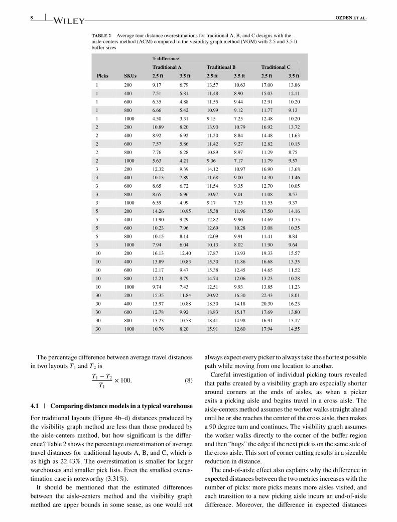
TABLE 2 Average tour distance overestimations for traditional A, B, and C designs with theaisle-centers method (ACM) compared to the visibility graph method (VGM) with 2.5 and 3.5 ftbuffer sizes

% difference

Traditional A Traditional B Traditional C

Picks SKUs 2.5 ft 3.5 ft 2.5 ft 3.5 ft 2.5 ft 3.5 ft

1 200 9.17 6.79 13.57 10.63 17.00 13.86

1 400 7.51 5.81 11.48 8.90 15.03 12.11

1 600 6.35 4.88 11.55 9.44 12.91 10.20

1 800 6.66 5.42 10.99 9.12 11.77 9.13

1 1000 4.50 3.31 9.15 7.25 12.48 10.20

2 200 10.89 8.20 13.90 10.79 16.92 13.72

2 400 8.92 6.92 11.50 8.84 14.48 11.63

2 600 7.57 5.86 11.42 9.27 12.82 10.15

2 800 7.76 6.28 10.89 8.97 11.29 8.75

2 1000 5.63 4.21 9.06 7.17 11.79 9.57

3 200 12.32 9.39 14.12 10.97 16.90 13.68

3 400 10.13 7.89 11.68 9.00 14.30 11.46

3 600 8.65 6.72 11.54 9.35 12.70 10.05

3 800 8.65 6.96 10.97 9.01 11.08 8.57

3 1000 6.59 4.99 9.17 7.25 11.55 9.37

5 200 14.26 10.95 15.38 11.96 17.50 14.16

5 400 11.90 9.29 12.82 9.90 14.69 11.75

5 600 10.23 7.96 12.69 10.28 13.08 10.35

5 800 10.15 8.14 12.09 9.91 11.41 8.84

5 1000 7.94 6.04 10.13 8.02 11.90 9.64

10 200 16.13 12.40 17.87 13.93 19.33 15.57

10 400 13.89 10.83 15.30 11.86 16.68 13.35

10 600 12.17 9.47 15.38 12.45 14.65 11.52

10 800 12.21 9.79 14.74 12.06 13.23 10.28

10 1000 9.74 7.43 12.51 9.93 13.85 11.23

30 200 15.35 11.84 20.92 16.30 22.43 18.01

30 400 13.97 10.88 18.30 14.18 20.30 16.23

30 600 12.78 9.92 18.83 15.17 17.69 13.80

30 800 13.23 10.58 18.41 14.98 16.91 13.17

30 1000 10.76 8.20 15.91 12.60 17.94 14.55

The percentage difference between average travel distancesin two layouts T1 and T2 is

T1 − T2

T1× 100. (8)

4.1 Comparing distance models in a typical warehouse

For traditional layouts (Figure 4b–d) distances produced bythe visibility graph method are less than those produced bythe aisle-centers method, but how significant is the differ-ence? Table 2 shows the percentage overestimation of averagetravel distances for traditional layouts A, B, and C, which isas high as 22.43%. The overestimation is smaller for largerwarehouses and smaller pick lists. Even the smallest overes-timation case is noteworthy (3.31%).

It should be mentioned that the estimated differencesbetween the aisle-centers method and the visibility graphmethod are upper bounds in some sense, as one would not

always expect every picker to always take the shortest possiblepath while moving from one location to another.

Careful investigation of individual picking tours revealedthat paths created by a visibility graph are especially shorteraround corners at the ends of aisles, as when a pickerexits a picking aisle and begins travel in a cross aisle. Theaisle-centers method assumes the worker walks straight aheaduntil he or she reaches the center of the cross aisle, then makesa 90 degree turn and continues. The visibility graph assumesthe worker walks directly to the corner of the buffer regionand then “hugs” the edge if the next pick is on the same side ofthe cross aisle. This sort of corner cutting results in a sizeablereduction in distance.

The end-of-aisle effect also explains why the difference inexpected distances between the two metrics increases with thenumber of picks: more picks means more aisles visited, andeach transition to a new picking aisle incurs an end-of-aisledifference. Moreover, the difference in expected distances

OZDEN ET AL. 9

TABLE 3 Average tour distance overestimations for traditional A, B, and C designs with the aisle-centers method (ACM) versus the visibility graphmethod (VGM) with 2.5 and 3.5 ft buffer sizes

Average tour distance (ft)

Traditional A Traditional B Traditional C Best to worst Penalty cost (%)

Picks SKUs ACM 2.5 3.5 ACM 2.5 3.5 ACM 2.5 3.5 ACM 2.5 ft 3.5 ft 2.5 ft 3.5 ft

1 200 141 128 132 162 140 145 175 145 151 A, B, C A, B, C A, B, C 0.0 0.0

1 400 194 179 183 210 186 191 229 194 201 A, B, C A, B, C A, B, C 0.0 0.0

1 600 234 219 222 255 225 231 266 231 238 A, B, C A, B, C A, B, C 0.0 0.0

1 800 274 255 259 293 261 267 297 262 270 A, B, C A, B, C A, B, C 0.0 0.0

1 1000 297 283 287 317 288 294 338 295 303 A, B, C A, B, C A, B, C 0.0 0.0

2 200 236 210 216 248 214 221 270 224 233 A, B, C A, B, C A, B, C 0.0 0.0

2 400 325 296 302 324 286 295 349 298 308 B, A, C B, A, C B, A, C 0.0 0.0

2 600 391 362 369 395 350 358 407 355 366 A, B, C B, C, A* B, C, A* 3.4 2.92 800 458 423 430 453 404 412 454 403 414 B, C, A C, B, A* B, C, A 0.3 0.0

2 1000 498 470 477 491 447 456 514 454 465 B, A, C B, C, A* B, C, A* 0.0 0.0

3 200 302 264 273 303 260 270 330 274 285 A, B, C B, A, C* B, A, C* 1.6 1.33 400 417 375 384 395 349 360 427 366 378 B, A, C B, C, A* B, C, A* 0.0 0.0

3 600 504 460 470 483 428 438 498 434 448 B, C, A B, C, A B, C, A 0.0 0.0

3 800 588 537 547 556 495 506 555 493 507 C, B, A C, B, A B, C, A* 0.0 0.33 1000 640 598 608 603 548 559 628 556 569 B, C, A B, C, A B, C, A 0.0 0.0

5 200 393 337 350 384 325 338 413 341 355 B, A, C B, A, C B, A, C 0.0 0.0

5 400 551 485 500 504 440 454 531 453 469 B, C, A B, C, A B, C, A 0.0 0.0

5 600 668 599 615 616 538 552 621 540 557 B, C, A B, C, A B, C, A 0.0 0.0

5 800 782 702 718 707 622 637 691 612 630 C, B, A C, B, A C, B, A 0.0 0.0

5 1000 851 784 800 767 689 706 783 690 707 B, C, A B, C, A B, C, A 0.0 0.0

10 200 542 455 475 523 430 451 553 446 467 B, A, C B, C, A* B, C, A* 0.0 0.0

10 400 779 671 695 690 584 608 711 593 616 B, C, A B, C, A B, C, A 0.0 0.0

10 600 958 841 867 851 720 745 835 713 739 C, B, A C, B, A C, B, A 0.0 0.0

10 800 1135 996 1024 978 834 860 923 801 828 C, B, A C, B, A C, B, A 0.0 0.0

10 1000 1238 1117 1146 1060 928 955 1050 905 932 C, B, A C, B, A C, B, A 0.0 0.0

30 200 758 642 669 797 630 667 872 677 715 A, B, C B, A, C* B, A, C* 1.8 0.230 400 1181 1016 1052 1105 903 948 1148 915 961 B, C, A B, C, A B, C, A 0.0 0.0

30 600 1538 1342 1386 1409 1144 1196 1370 1128 1181 C, B, A C, B, A C, B, A 0.0 0.0

30 800 1887 1637 1687 1654 1349 1406 1524 1266 1323 C, B, A C, B, A C, B, A 0.0 0.0

30 1000 2114 1887 1941 1818 1529 1589 1754 1440 1499 C, B, A C, B, A C, B, A 0.0 0.0

increases with a smaller buffer size (2.5 ft vs. 3.5 ft) becauseof greater flexibility of taking shortcuts. In other words, ahuman worker with a cart can take a shorter path because ofhis or her size compared to a forklift or automated guidedvehicle. Finally, percent differences tend to go down as thesize of the warehouse increases: as aisles get longer, more ofeach tour is within aisles and corner cutting comprises less ofthe overall distance.

4.2 Traditional design using the visibility graphversus aisle-centers with fixed pick list size

Choosing the number and orientation of cross aisles in a lay-out requires finding a design that minimizes expected traveldistance. With a model based on visibility graphs instead ofaisle-centers, should we expect different design decisions?

We consider this question in the context of layouts withparallel picking aisles and orthogonal cross aisles (so-called

“traditional designs”). Table 3 shows best to worst ranking oftraditional layouts A, B, and C with each method (“*” indi-cates that best to worst layout ranking order has changed).Smaller warehouses have a larger percentage gap in averagetour distance between the aisle-centers method and the visibil-ity graph method. 7 out of 30 best to worst rankings change forboth 2.5 and 3.5 ft buffer sizes. More importantly, in 13.3% ofthe cases the best layout with respect to average tour distancechanges for both 2.5 and 3.5 ft buffer sizes. For these cases,the difference in estimated travel distance is between 0.2 and3.4%. The penalty of choosing a design using aisle-centers isnonzero only when the best layout changes between the twodistance estimation methods.

As an added analysis, we considered a small example tosee if and how the ordering of the picks changes by using thevisibility graph method. We considered a small warehouse oftraditional B design with 200 SKUs and 10 pick lists with eachpick list of 5 items. This warehouse has 12 ft cross aisle and

10 OZDEN ET AL.

TABLE 4 Three sets of actual pick list (PL) data

PL set#Numberof SKUs

Numberof PLs

Averagenumber ofSKUs per PL

1 597 4625 7.93

2 510 4957 7.40

3 267 98 10.21

TABLE 5 Warehouse parameters used for the computational experimentsfor variable pick list data

PL set# LayoutNumber oflocations Area

Aspectratio

Pickaisleangles

1 Traditional A 598 33,811 0.50 90

1 Traditional B 600 38,662 0.50 90, 90

1 Traditional C 600 41,800 0.54 90, 90, 90

2 Traditional A 520 30,746 0.55 90

2 Traditional B 528 34,322 0.50 90, 90

2 Traditional C 525 38,662 0.50 90, 90, 90

3 Traditional A 272 17,681 0.50 90

3 Traditional B 272 20,812 0.50 90, 90

3 Traditional C 285 24,994 0.52 90, 90, 90

pick aisles and 4 ft wide and deep storage locations. The picklists were generated using Benders Model and all items haveuniform demand (i.e., each item has an equal probability ofbeing picked). All items were allocated to the same locationsin both the visibility graph and aisle-centers methods. Fromthe solution files of Concorde TSP solver for each of 10 picklists and found that 8 out of 10 pick lists had a different optimalsequence to pick the items on the pick list.

4.3 Traditional design using the visibility graphversus aisle-centers with variable pick list size

In previous section, we have used fixed size generated picklists for comparison. Even though it is useful analysis on thecomparative efficiency of these layouts, the design of thewarehouse is not determined based on a single pick list sizeunless it is a single-command or a dual-command system.Therefore, we extended the analysis of the previous sectionby using actual pick list data which has combinations of dif-ferent pick list sizes (see Table 4). We compared the samethree traditional designs from previous section. We used threedifferent set of pick lists from real data. Table 5 shows thewarehouse design parameters for each set of pick lists.

Table 6 shows best to worst ranking of traditional layoutsA, B, and C with each method (“*” indicates that best to worstlayout ranking order has changed). Similar to the previousexperiment with uniform pick list sizes, smaller warehouseshave a larger percentage gap in average tour distance betweenthe aisle-centers method and the visibility graph method. Inone out of three cases, the preferred layout with respect toaverage tour distance changes for both 2.5 and 3.5 ft buffersizes changes. For these cases, the difference in estimatedtravel distance is between 3.7 and 4.6%.

4.4 Fishbone design using the visibility graph versusaisle-centers

Even a cursory look at the geometry of visibility graphssuggests important differences from the aisle-centers methodwhen picking and cross aisles meet at other than right angles.Specifically, when a worker must turn more than 90 degrees,the aisle-centers method assumes the worker travels an unrea-sonable path, whereas a visibility graph represents a morereasonable path. Conversely, if a worker turns into an aisleat, say, 45 degrees, then the aisle-centers and visibility graphmethods produce similar, though not identical, distances.

For single-command, unit-load operations in a fishbonedesign, pickers make turns only at 45 degrees, and so there isless advantage to cutting a corner. This observation suggeststhat the difference between the aisle-centers and visibilitygraph methods should be less for a fishbone design thanfor a traditional design. For tours with more than one pick,workers will sometimes have to turn more than 90 degrees ina fishbone design, so we expect the difference in average dis-tance between the visibility graph and aisle-centers methodsto increase.

To investigate these questions, we consider a fishbone andtraditional design B with the parameters in Table 7. Aspectratio is the ratio of depth to the width of the warehouse. A 0.5aspect ratio means that the warehouse is twice as wide as deep.Traditional Layout B has two regions and each region has 90degree pick aisles. The fishbone layout has three regions. Theleft and right regions have 0 degree pick aisles and the mid-dle region has 90 degree pick aisles. For many warehouses,the customer demand distribution is skewed. Therefore, inthis section we also consider cases in which demand is notuniform. Figure 10 shows the results for uniform demandand for 20 of 40, 20 of 60, and 20 of 80 demand skewness.For single-command operations, the fishbone layout’s perfor-mance improvement over traditional layout B decreases from18.17 to 15.12% (2.5 ft buffer) and 15.87% (3.5 ft buffer)when using the visibility graph method, as expected. As thesize of the pick list increases, the aisle-centers method pro-duces longer distances relative to the visibility graph, sothe percent improvement of a fishbone design is lower, andeventually negative. The results are similar for all values ofdemand skewness.

4.5 The effect of the warehouse size in percentimprovement of fishbone layouts

In a final set of experiments, we analyze the percent improve-ment of the fishbone layout over traditional layout A (seeFigure 4b) for unit-load (i.e., single command) operations anddifferent warehouse sizes. We use traditional layout A insteadof traditional layout B because addition of the middle aisleof traditional layout B has no benefit for unit-load operations(Gue & Meller, 2009). This set of experiments is similar to thediscrete model analysis performed by Öztürkoglu et al. (2012)

OZDEN ET AL. 11

TABLE 6 Average tour distance overestimations for traditional A, B, and C designs with the aisle-centers method (ACM) versus the visibility graph method(VGM) with 2.5 and 3.5 ft buffer sizes with variable pick list data sets

Average tour distance (ft)

Traditional A Traditional B Traditional C Best to worst Penalty cost (%)

PL set ACM 2.5 3.5 ACM 2.5 3.5 ACM 2.5 3.5 ACM 2.5 ft 3.5 ft 2.5 ft 3.5 ft

1 451 411 420 544 470 486 542 463 481 A, C, B A, C, B A, C, B 0.0 0.0

2 434 396 405 478 407 422 491 410 427 A, B, C A, B, C A, B, C 0.0 0.0

3 390.9 345 356 391 329 343 477 393 411 A, B, C B, A, C B, A, C 4.6 3.7

TABLE 7 Warehouse parameters used for the fishbone experiments

Layout Number of locations Area Aspect ratio Pick aisle angles

Traditional B 4012 191,260 0.51 90, 90

Fishbone 4000 196,109 0.50 0, 90, 0

1 2 3 5 10 30− 20

− 10

0

10

20

30

Pick List Size

%Im

provem

entover

Traditional

B

Uniform Demand

Aisle-centers

Visibility Graph 2.5ft.

Visibility Graph 3.5ft.

1 2 3 5 10 30− 20

− 10

0

10

20

30

Pick List Size

%Im

provem

entover

Traditional

B

20/40

Aisle-centers

Visibility Graph 2.5ft.

Visibility Graph 3.5ft.

1 2 3 5 10 30− 20

− 10

0

10

20

30

Pick List Size

%Im

provem

entover

Traditional

B

20/60

Aisle-centers

Visibility Graph 2.5ft.

Visibility Graph 3.5ft.

1 2 3 5 10 30− 20

− 10

0

10

20

30

Pick List Size

%Im

provem

entover

Traditional

B

20/80

Aisle-centers

Visibility Graph 2.5ft.

Visibility Graph 3.5ft.

FIGURE 10 The change in relative fishbone percent improvement over traditional layout B as pick list size increases

and Pohl et al. (2011). Figure 11 shows the results. Thecurves in Figure 11 are not smooth because as warehouse size(number of SKUs) increases, the number of picking aislesin the fishbone and traditional layout A warehouses changediscretely and independently of one another. For small ware-houses, the difference between the two distance models is ashigh as 5.89%. As the size of the warehouse increases, the dif-ference between the two metrics decreases because a greaterpercentage of travel is within aisles and not between them.

5 CONCLUSIONS

Although we have not made the case with observational data,we contend that a properly established visibility graph better

represents travel paths associated with reasonable workerbehavior in order picking warehouses. The traditional modelof distances based on aisle-centers assumes that workers walkto the center of picking and cross aisles and then (assuminga traditional design) make right angle turns to continue. Thevisibility graph assumes workers will make reasonable effortsto cut corners and therefore take shorter paths to their des-tinations. We have shown analytically and empirically thatusing the aisle-centers method overestimates the distance thata rational worker would walk.

The implications of this new approach are significant. First,it suggests that travel distances between locations in a ware-house are not as long as commonly assumed and thereforethat associated labor costs are not as high. Said another way,throughput for a given number of pickers should be higher

12 OZDEN ET AL.

2000 4000 6000 80006

8

10

12

14

16

18

Warehouse Size (Number of SKUs)

%Im

provem

entover

Traditional

A

Aisle-centers

Visibility Graph 2.5 ft.

Visibility Graph 3.5 ft.

FIGURE 11 Percent improvement of a fishbone design over traditional

layout A for single-command unit-load operations and different warehouse

sizes

than predicted by the traditional model because workers travelshorter paths than the model assumes.

Second, preferred warehouse designs based on the new dis-tance estimation model can be different that those based onthe aisle-centers method. In 13.3% of the cases we considered,the selected traditional layout was different when using a vis-ibility graph distance metric. An interesting follow-on studycould consider nontraditional designs with diagonal aislesusing the visibility graph during the warehouse design phase.

Third, our results suggest that the previous results of Gueand Meller (2009) and Çelik and Süral (2014) over-estimatethe potential benefit of diagonal aisles versus traditional lay-outs for unit-load and order picking operations. This is notto say that these designs do not offer benefit, only that thelevel of benefit is probably not as high as their original modelssuggest.

As future work, we can ‘smooth’ the corners of thepaths using a Bezier interpolation which takes turning radiiinto account and provide more accurate distance measures.Another major step forward would be a human study con-ducted in warehouse environments to ascertain the degree ofnatural corner cutting by workers.

ACKNOWLEDGMENTThis research was supported in part by the National ScienceFoundation under grant CMMI-1200567. Any opinions, find-ings, and conclusions or recommendations expressed in thismaterial are those of the authors and do not necessarily reflectthe views of the National Science Foundation. The authorswould like to thank Dr. Aleksandr Vinel for his contributionsto some of the analytical results and to undergraduate andgraduate research assistants Michael Robbins, Ataman Billor,and Akhil Varma Jampana for data collection and testing thecode. Source code and binary files can be downloaded fromhttps://github.com/gokhanozden/gabak.

ORCID

Sabahattin G. Ozden https://orcid.org/0000-0002-5005-0298Alice E. Smith https://orcid.org/0000-0001-8808-0663Kevin R. Gue https://orcid.org/0000-0002-9438-2788

REFERENCES

Altarazi, S. A., & Ammouri, M. M. (2018). Concurrent

manual-order-picking warehouse design: A simulation-based design

of experiments approach. International Journal of ProductionResearch, 56(23), 7103–7121.

Applegate, D. L., Bixby, R. E., Chvatal, V., & Cook, W. J. (2007). The

traveling salesman problem: A computational study. Princeton, NJ:

Princeton University Press.

Bellman, R. (1958). On a routing problem. Quarterly of Applied Math-ematics, 16, 87–90.

Canny, J., & Reif, J. (1987). New lower bound techniques for robotmotion planning problems. In Proceedings of the 28th annual sympo-

sium on foundations of computer science (pp. 49–60). Los Alamitos,

CA: IEEE Computer Society Press.

Çelik, M., & Süral, H. (2014). Order picking under random and

turnover-based storage policies in fishbone aisle warehouses. IIETransactions, 46(3), 283–300.

Çelik, M., & Süral, H. (2019). Order picking in parallel-aisle warehouses

with multiple blocks: Complexity and a graph theory-based heuris-

tic. International Journal of Production Research, 57(3), 888–906.

Dijkstra, A. S., & Roodbergen, K. J. (2017). Exact route-length formu-

las and a storage location assignment heuristic for picker-to-parts

warehouses. Transportation Research Part E: Logistics and Trans-portation Review, 102, 38–59.

Dijkstra, E. W. (1959). A note on two problems in connexion.

Numerische Mathematik, 1, 269–271.

Floyd, R. W. (1962). Algorithm 97: Shortest path. Communications ofthe ACM, 5(6), 345.

Ford, L. R. (1956). Network flow theory. Tech. rep. The Rand Corpora-

tion.

Gallo, G., & Pallottino, S. (1986). Shortest path methods: A unifyingapproach. In Netflow at Pisa (pp. 38–64). Berlin: Springer.

Ghosh, S. K., & Mount, D. M. (1991). An output-sensitive algorithm

for computing visibility graphs. SIAM Journal on Computing, 20(5),

888–910.

Goetschalckx, M., & Ratliff, H. D. (1988). Order picking in an aisle. IIETransactions, 20, 53–62.

Gue, K. R., & Meller, R. D. (2009). Aisle configurations for unit-load

warehouses. IIE Transactions, 41(3), 171–182.

Habbal, M. B., Koutsopoulos, H. N., & Lerman, S. R. (1994). A

decomposition algorithm for the all-pairs shortest path problem on

massively parallel computer architectures. Transportation Science,

28(4), 292–308.

Hall, R. W. (1993). Distance approximation for routing manual pickers

in a warehouse. IIE Transactions, 25(4), 76–87.

Hart, P. E., Nilsson, N. J., & Raphael, B. (1968). A formal basis for the

heuristic determination of minimum cost paths. IEEE Transactionson Systems Science and Cybernetics, 4(2), 100–107.

Hershberger, J., & Suri, S. (1999). An optimal algorithm for euclidean

shortest paths in the plane. SIAM Journal on Computing, 28(6),

2215–2256.

Johnson, D. B. (1977). Efficient algorithms for shortest paths in sparse

networks. Journal of the ACM (JACM), 24(1), 1–13.

OZDEN ET AL. 13

Lozano-Pérez, T., & Wesley, M. A. (1979). An algorithm for planningcollision-free paths among polyhedral obstacles. Communications ofthe ACM, 22(10), 560–570.

Moore, E. F. (1959). The shortest path through a maze. In Proc. inter-national symposium on the theory of switching (pp. 285–292). Har-vard: Harvard University Press http://ci.nii.ac.jp/naid/10010192763/en/.

Moy, J., 1994. Open shortest path first version 2. rfq 1583. InternetEngineering Task Force. Retrieved from http://www.ietf.org/

Öztürkoglu, Ö., Gue, K. R., & Meller, R. D. (2012). Optimal unit-loadwarehouse designs for single-command operations. IIE Transac-tions, 44(6), 459–475.

Petersen, C. G. (1999). The impact of routing and storage policieson warehouse efficiency. International Journal of Operations &Production Management, 19, 1053–1064.

Peyer, S., Rautenbach, D., & Vygen, J. (2009). A generalization of Dijk-stra’s shortest path algorithm with applications to VLSI routing.Journal of Discrete Algorithms, 7(4), 377–390.

Pohl, L. M., Meller, R. D., & Gue, K. R. (2009a). An analysis ofdual-command operations in common warehouse designs. Trans-portation Research Part E: Logistics and Transportation Review, 45,367–379.

Pohl, L. M., Meller, R. D., & Gue, K. R. (2009b). Optimizing fishboneaisles for dual-command operations in a warehouse. Naval ResearchLogistics, 56(5), 389–403.

Pohl, L. M., Meller, R. D., & Gue, K. R. (2011). Turnover-based stor-age in non-traditional unit-load warehouse designs. IIE Transactions,43(10), 703–720.

Ratliff, H. D., & Rosenthal, A. S. (1983). Order-picking in a rectangu-lar warehouse: A solvable case of the traveling salesman problem.Operations Research, 31, 507–521.

Roodbergen, K. J., & De Koster, R. (2001a). Routing methods forwarehouses with multiple cross aisles. International Journal of Pro-duction Research, 39, 1865–1883.

Roodbergen, K. J., & De Koster, R. (2001b). Routing order pickers ina warehouse with a middle aisle. European Journal of OperationalResearch, 133(1), 32–43.

Roodbergen, K. J., Sharp, G. P., & Vis, I. F. (2008). Designing thelayout structure of manual order picking areas in warehouses. IIETransactions, 40(11), 1032–1045.

Roodbergen, K. J., & Vis, I. F. A. (2006). A model for warehouse layout.IIE Transactions, 38(10), 799–811.

Soueres, P., & Laumond, J.-P. (1996). Shortest paths synthesis fora car-like robot. IEEE Transactions on Automatic Control, 41(5),672–688.

Theys, C., Bräysy, O., Dullaert, W., & Raa, B. (2010). Using a TSPheuristic for routing order pickers in warehouses. European Journalof Operational Research, 200, 755–763.

Toth, C. D., O’Rourke, J., & Goodman, J. E. (2004). Handbook ofdiscrete and computational geometry. Boca Raton, FL: CRC Press.

Zhan, F. B., & Noon, C. E. (1998). Shortest path algorithms: Anevaluation using real road networks. Transportation Science, 32(1),65–73.

How to cite this article: Ozden SG, Smith AE,Gue KR. A novel approach for modeling orderpicking paths. Naval Research Logistics 2020;1–14.https://doi.org/10.1002/nav.21966

APPENDIX A

In this appendix we derive closed forms expressions for theexpected travel distance between two random locations for thevisibility graph method and compare this to the same value forthe aisle-centers method from the work of Pohl et al. (2009a).Then, we calculate the expected difference between them, andthus the overestimation of the aisle-centers method.

We divide the travel distance into two components:cross aisle travel and picking aisle travel (as does Pohlet al. (2009a)). We assume the locations are uniformly dis-tributed among the aisles. All aisles are equally likely tocontain one of the two locations because of the uniform dis-tribution. There are n2 possible combinations of i and j forn number of aisles (all locations are equally likely to bepicked). There are n possible ways that i = j, for which nocross aisle travel is required. The probability that |i = j| = 0is n/n2. Similarly, there are 2(n− 1) combinations of |i− j|,so Pr(|i− j| = 1) = 2(n− 1)/n2. Unlike Pohl et al. (2009a),we have a special case where the cross aisle distance is 2bwhen |i− j| = 1 instead of 2a+ 2b as in Pohl et al. (2009a).Therefore we directly calculate the expected cross aisle traveldistance instead of first calculating the expected number ofaisle widths between i and j (which is not uniform for all iand j values). Considering the special case, the expected crossaisle travel distance for the visibility graph (for n> 0) is

E[TBcrossaisle] =n−1∑k=1

2(n − k)n2

(2b + (k − 1)(2a + 2b))

= 2(n − 1)(a(n − 2) + b(n + 1))3n

(A1)

For picking aisle travel using the visibility graph, thereare two cases: two locations are in the same picking aisleand two locations are in different picking aisles. Since weassume a continuous uniform distribution within each aisle,we let Xi and Yj be uniform random variables that representthe positions of the locations in aisles i and j, respectively,where Xj ∼U(0, L) and Yj U(0, L). From probability theory,we know the expected distance between two locations on thesame aisle of length L is E[|x− y|] = L/3. For the second casewhere locations are on different aisles, the picking aisle travel

distance is min[√

x2 + a2 +√

y2 + a2,√(L − x)2 + (L − y)2].

Then,

f1(a,L) = E[min

[√y2 + a2,

√(L − x)2 + (L − y)2

]]= 1

12L2

(16a3 − 16a2

√a2 + L2 + 8L2

√a2 + L2

+ 3a2LArchTanh

[L√

a2 + L2

]

− 15a2LLog

[a

L +√

a2 + L2

]

+ 6a2LLog

[L +

√a2 + L2

a

])(A2)

14 OZDEN ET AL.

TABLE A1 Expected travel between distances by visibility graph (VG) and aisle-centers method (ACM), simulation results and absolutepercentage difference between E[TBVG] and simulation, and the overestimation of the ACM for various warehouse parameters

a L n v b E[TBVG] Simulation % Diff E[TBACM] Overestimation (%)

6 6 1 6 4 2.00 2.00 0.00 2.00 0.00

6 6 1 6 2 2.00 2.00 0.00 2.00 0.00

6 6 1 6 1 2.00 2.00 0.00 2.00 0.00

6 6 2 6 4 11.46 11.46 0.02 19.00 39.69

6 6 2 6 2 9.46 9.47 0.13 17.00 44.35

6 6 2 6 1 8.46 8.46 0.05 16.00 47.13

6 6 50 6 4 334.14 334.88 0.22 348.92 4.24

6 6 50 6 2 267.50 266.54 0.36 282.28 5.24

6 6 50 6 1 234.18 234.32 0.06 248.96 5.94

6 240 1 6 4 80.00 80.00 0.00 80.00 0.00

6 240 1 6 2 80.00 80.00 0.00 80.00 0.00

6 240 1 6 1 80.00 80.00 0.00 80.00 0.00

6 240 2 6 4 124.58 124.64 0.05 136.00 8.39

6 240 2 6 2 122.58 122.71 0.10 134.00 8.52

6 240 2 6 1 121.58 122.02 0.35 133.00 8.58

6 240 50 6 4 480.99 480.38 0.13 503.36 4.44

6 240 50 6 2 414.35 413.48 0.21 436.72 5.12

6 240 50 6 1 381.03 381.73 0.18 403.40 5.55

The probability the second location will be in the same aisleas the first location (i.e, |i− j| = 0) is 1/n, and the probabilitythe second location will be in a different aisle (n− 1)/n. Theexpected picking aisle travel distance is then

1n

(L3

)+ n − 1

nf1(a,L) (A3)

To compare this quantity for different warehouse sizes wecalculate the values in Table A1 and also verify the analytical

results for the visibility graph with simulation. Simulationexperiments are done based on 100,000 trials. The resultsrange from no overestimation to nearly 50%. The simula-tion results provide nearly total agreement with the analyticequations derived in this appendix.