A note on the Brownian loop measure

Gregory F. Lawler

Department of Mathematics

University of Chicago ∗

March 23, 2009

Abstract

The Brownian loop measure is a conformally invariant measureon loops that also satisfies the restriction property. In studying theSchramm-Loewner evolution (SLE), a quantity that arises is the mea-sure of loops in a domain D that intersect both V1 and V2. If V1, V2

are nonpolar, and D = C this measure is infinite. We show the ex-istence of a finite normalized quantity that can be used in its place.The motivation for studying this question comes from bulk SLE withboundary conditions, but this paper only discusses the loop measure.

1 Introduction

The Brownian loop measure [4] in C is a sigma-finite measure on unrootedloops in C that satisfies two important properties: conformal invariance andthe restriction property. It arose in the study of the Schramm-Loewnerevolution (SLE). An important quantity for SLE is

Λ(V1, V2;D),

which denotes the measure of the set of loops in a domain D that intersectboth V1 and V2. This quantity comes up in comparison of SLE in twodifferent domains. If µD(z1, z2) denotes the chordal SLEκ (κ ≤ 4) measurefor z1 to z2 in a domain D and D ⊂ D is a subdomain that agrees with Din neighborhoods of z1 and z2, then

dµD(z1, z2)

dµD(z1, z2)(γ) = exp

{c

2Λ(γ,D \ D;D)

}

,

∗Research supported by National Science Foundation grant DMS-0734151.

1

where

c =(3κ − 8)(6 − κ)

2κ

denotes the central charge.If V1, V2 are nonpolar disjoint closed subsets of the Riemann sphere and

D is a domain whose boundary is nonpolar, then this quantity is positiveand finite (see Corollary 4.6). It is also conformally invariant in the sensethat if f : D → f(D) is a conformal transformation, then

Λ(f(V1), f(V2); f(D)) = Λ(V1, V2;D).

In trying to generalize these ideas to SLE in the bulk, see [2], one istempted to write similar quantities of the form

Λ(V1, V2; C).

However this quantity as defined is infinite. The purpose of this note is toprove the existence of a normalized quantity Λ∗(V1, V2) that has many ofthe properties one wants.

Theorem 1.1. If V1, V2 are disjoint nonpolar closed subsets of the Riemannsphere, then the limit

Λ∗(V1, V2) = limr→0+

[Λ(V1, V2;Or) − log log(1/r)], (1)

exists whereOr = {z ∈ C : |z| > r}.

Moreover, if f is a Mobius transformation of the Riemann sphere,

Λ∗(f(V1), f(V2)) = Λ∗(V1, V2).

We could write the assumption “disjoint nonpolar closed subsets of theRiemann sphere” as “disjoint closed subsets of C, at least one of which iscompact, such that Brownian motions hits both subsets at some positivetime”.

Invariance of Λ∗ under Mobius transformations implies that the defini-tion (1) does not change if we shrink down at a point on the Riemann sphereother than the origin. In other words if Or(z) = z +Or and DR denotes theopen disk of radius R about the origin,

Λ∗(V1, V2) = limr→0+

[Λ(V1, V2;Or(z)) − log log(1/r)], (2)

2

Λ∗(V1, V2) = limR→∞

[Λ(V1, V2; DR) − log log R]. (3)

The goal of this paper is to prove Theorem 1.1. Theorem 4.7 establishesthe existence of the limit in (1). Theorem 4.11 proves the alternate forms(2) and (3). If f is a Mobius transformation, then conformal invariance ofthe loop measure implies

Λ(V1, V2;Or) = Λ(f(V1), f(V2); f(Or)).

Invariance of Λ∗ under dilations, translations, and inversions can be deducedfrom this and (1), (2), and (3), respectively.

The proof really only uses standard arguments about planar Brownianmotion but we need to control the error terms. In order to make the papereasier to understand, we have split it into three sections. The first sectionconsiders estimates for planar Brownian motion. Readers who are well ac-quainted with planar Brownian motion may wish to skip this section andrefer back as necessary. This section does assume knowledge of planar Brow-nian motion as in [1, Chapter 2]. The next section discusses the Brownian(boundary) bubble measure and gives estimates for it. The Brownian loopmeasure is a measure on unrooted loops, but for computational purposes itis often easier to associate to each unrooted loop a particular rooted loopyielding an expression in terms of Brownian bubbles. The last section provesthe main theorem by giving estimates for the loop measure.

We will use the following notation:

Dr = {z : |z| < r}, D = D1,

Or = {z : |z| > r}, O = O1, Or(w) = w + Or,

Ar,R = DR ∩Or = {z : r < |z| < R}, AR = A1,R,

Cr = ∂Dr = ∂Or = {|z| = r}, Cr(w) = ∂Or(w) = {z : |w − z| = r}.

We say that a subset V of C is nonpolar if it is hit by Brownian motion.More precisely, V is nonpolar if for every z ∈ C, the probability that aBrownian motion starting at z hits V is positive. Since Brownian motion isrecurrent we can replace “is positive” with “equals one”. For convenience,we will call a domain (connected open subset) D of C nonpolar if ∂D isnonpolar.

3

2 Lemmas about Brownian motion

If Bt is a complex Brownian motion and D is a domain, let

τD = inf{t : Bt 6∈ D}.

A domain D is nonpolar if and only if Pz{τD < ∞} = 1 for every z. In thiscase we define harmonic measure of D at z ∈ D by

hD(z, V ) = Pz{BτD∈ V }.

If V is smooth then we can write

hD(z, V ) =

∫

VhD(z,w) |dw|,

where hD(z,w) is the Poisson kernel. If z ∈ ∂D \V and ∂D is smooth nearz, we define the excursion measure of V in D from z by

ED(z, V ) = E(z, V ;D) = ∂nhD(z, V ),

where n = nz,D denotes the unit inward normal at z. If V is smooth, wecan write

ED(z, V ) =

∫

Vh∂D(z,w) |dw|,

where h∂D(z,w) := ∂nhD(z,w) is the excursion or boundary Poisson kernel.(Here the derivative ∂n is applied to the first variable.) One can also obtainthe excursion Poisson kernel as the normal derivative in both variables ofthe Green’s function; this establishes symmetry, h∂D(z,w) = h∂D(w, z). Iff : D → f(D) is a conformal transformation, then (assuming smoothness off at boundary points at which f ′ is taken)

hD(z, V ) = hf(D)(f(z), f(V )),

hD(z,w) = |f ′(w)|hf(D)(f(z), f(w)),

ED(z, V ) = |f ′(w)| Ef(D)(f(z), f(V )),

h∂D(z,w) = |f ′(z)| |f ′(w)|h∂f(D)(f(z), f(w)).

The exact form of the Poisson kernel in the unit disk shows that thereis a c such that for all |z| ≤ 1/2, |w| = 1

|2π hD(z,w) − 1| ≤ c |z|.

4

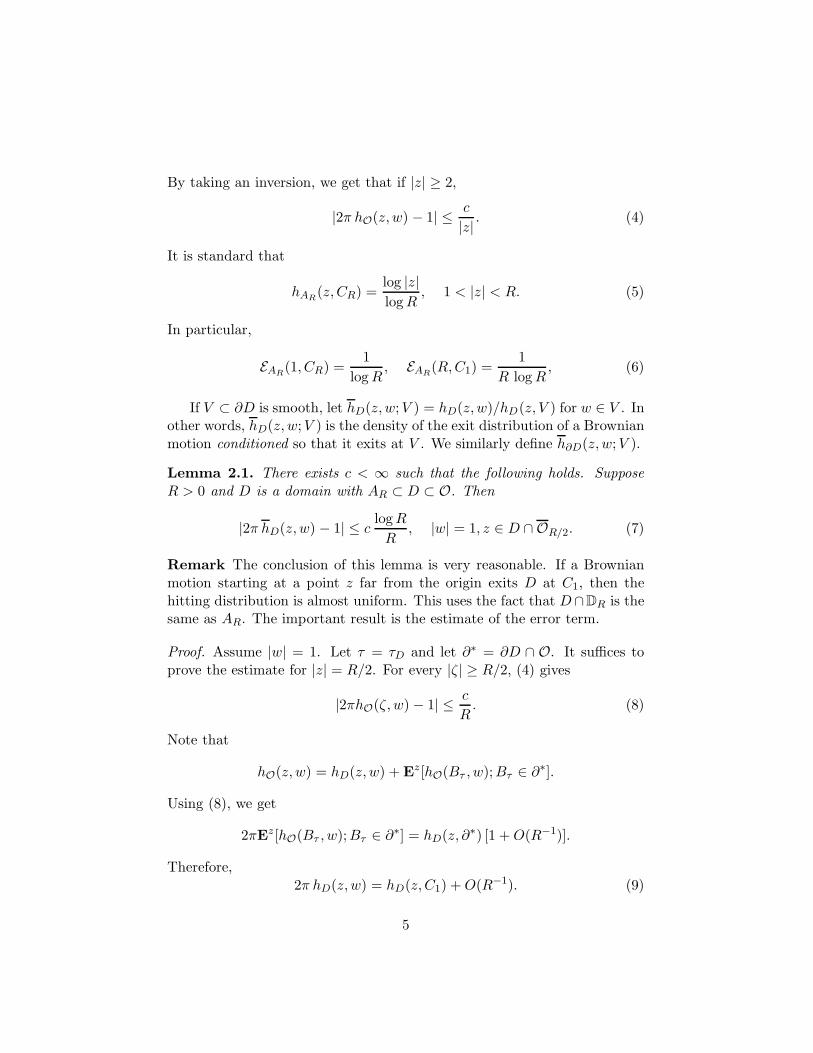
By taking an inversion, we get that if |z| ≥ 2,

|2π hO(z,w) − 1| ≤c

|z|. (4)

It is standard that

hAR(z,CR) =

log |z|

log R, 1 < |z| < R. (5)

In particular,

EAR(1, CR) =

1

log R, EAR

(R,C1) =1

R log R, (6)

If V ⊂ ∂D is smooth, let hD(z,w;V ) = hD(z,w)/hD(z, V ) for w ∈ V . Inother words, hD(z,w;V ) is the density of the exit distribution of a Brownianmotion conditioned so that it exits at V . We similarly define h∂D(z,w;V ).

Lemma 2.1. There exists c < ∞ such that the following holds. SupposeR > 0 and D is a domain with AR ⊂ D ⊂ O. Then

|2π hD(z,w) − 1| ≤ clog R

R, |w| = 1, z ∈ D ∩ OR/2. (7)

Remark The conclusion of this lemma is very reasonable. If a Brownianmotion starting at a point z far from the origin exits D at C1, then thehitting distribution is almost uniform. This uses the fact that D∩DR is thesame as AR. The important result is the estimate of the error term.

Proof. Assume |w| = 1. Let τ = τD and let ∂∗ = ∂D ∩ O. It suffices toprove the estimate for |z| = R/2. For every |ζ| ≥ R/2, (4) gives

|2πhO(ζ, w) − 1| ≤c

R. (8)

Note that

hO(z,w) = hD(z,w) + Ez[hO(Bτ , w);Bτ ∈ ∂∗].

Using (8), we get

2πEz[hO(Bτ , w);Bτ ∈ ∂∗] = hD(z, ∂∗) [1 + O(R−1)].

Therefore,2π hD(z,w) = hD(z,C1) + O(R−1). (9)

5

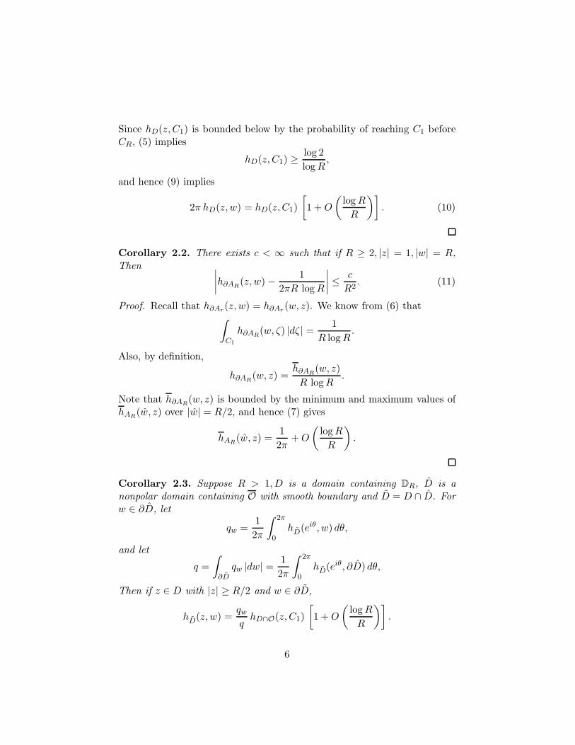
Since hD(z,C1) is bounded below by the probability of reaching C1 beforeCR, (5) implies

hD(z,C1) ≥log 2

log R,

and hence (9) implies

2π hD(z,w) = hD(z,C1)

[

1 + O

(

log R

R

)]

. (10)

Corollary 2.2. There exists c < ∞ such that if R ≥ 2, |z| = 1, |w| = R,Then

∣

∣

∣

∣

h∂AR(z,w) −

1

2πR log R

∣

∣

∣

∣

≤c

R2. (11)

Proof. Recall that h∂Ar(z,w) = h∂Ar (w, z). We know from (6) that∫

C1

h∂AR(w, ζ) |dζ| =

1

R log R.

Also, by definition,

h∂AR(w, z) =

h∂AR(w, z)

R log R.

Note that h∂AR(w, z) is bounded by the minimum and maximum values of

hAR(w, z) over |w| = R/2, and hence (7) gives

hAR(w, z) =

1

2π+ O

(

log R

R

)

.

Corollary 2.3. Suppose R > 1,D is a domain containing DR, D is anonpolar domain containing O with smooth boundary and D = D ∩ D. Forw ∈ ∂D, let

qw =1

2π

∫ 2π

0hD(eiθ, w) dθ,

and let

q =

∫

∂Dqw |dw| =

1

2π

∫ 2π

0hD(eiθ, ∂D) dθ,

Then if z ∈ D with |z| ≥ R/2 and w ∈ ∂D,

hD(z,w) =qw

qhD∩O(z,C1)

[

1 + O

(

log R

R

)]

.

6

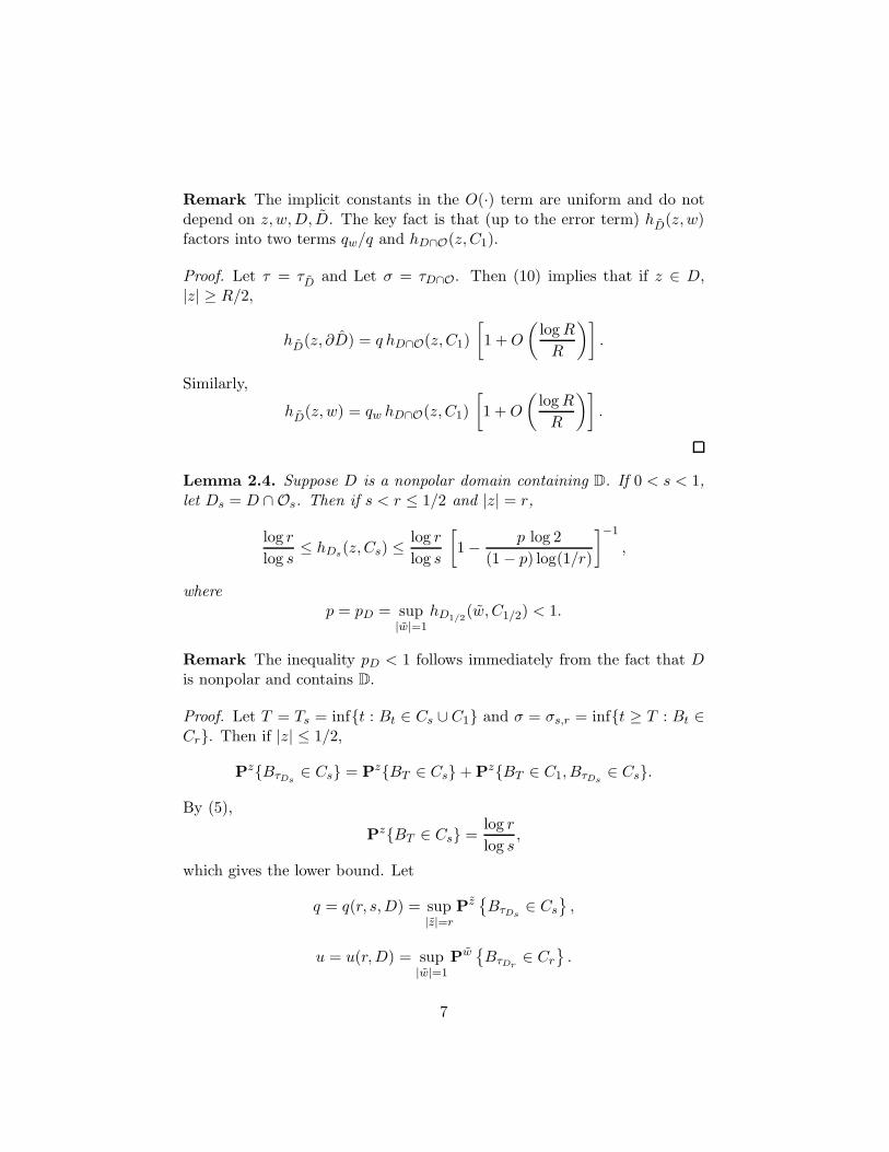
Remark The implicit constants in the O(·) term are uniform and do notdepend on z,w,D, D. The key fact is that (up to the error term) hD(z,w)factors into two terms qw/q and hD∩O(z,C1).

Proof. Let τ = τD and Let σ = τD∩O. Then (10) implies that if z ∈ D,|z| ≥ R/2,

hD(z, ∂D) = q hD∩O(z,C1)

[

1 + O

(

log R

R

)]

.

Similarly,

hD(z,w) = qw hD∩O(z,C1)

[

1 + O

(

log R

R

)]

.

Lemma 2.4. Suppose D is a nonpolar domain containing D. If 0 < s < 1,let Ds = D ∩ Os. Then if s < r ≤ 1/2 and |z| = r,

log r

log s≤ hDs(z,Cs) ≤

log r

log s

[

1 −p log 2

(1 − p) log(1/r)

]−1

,

wherep = pD = sup

|w|=1hD1/2

(w, C1/2) < 1.

Remark The inequality pD < 1 follows immediately from the fact that Dis nonpolar and contains D.

Proof. Let T = Ts = inf{t : Bt ∈ Cs ∪ C1} and σ = σs,r = inf{t ≥ T : Bt ∈Cr}. Then if |z| ≤ 1/2,

Pz{BτDs∈ Cs} = Pz{BT ∈ Cs} + Pz{BT ∈ C1, BτDs

∈ Cs}.

By (5),

Pz{BT ∈ Cs} =log r

log s,

which gives the lower bound. Let

q = q(r, s,D) = sup|z|=r

Pz{

BτDs∈ Cs

}

,

u = u(r,D) = sup|w|=1

Pw{

BτDr∈ Cr

}

.

7

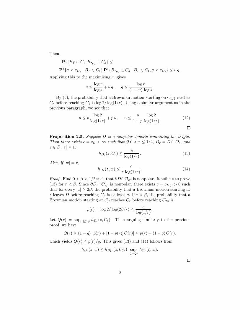
Then,

Pz{BT ∈ C1, BτDs∈ Cs} ≤

Pz{σ < τDs | BT ∈ C1}Pz{BτDs∈ Cs | BT ∈ C1, σ < τDs} ≤ u q.

Applying this to the maximizing z, gives

q ≤log r

log s+ u q, q ≤

log r

(1 − u) log s.

By (5), the probability that a Brownian motion starting on C1/2 reachesCr before reaching C1 is log 2/ log(1/r). Using a similar argument as in theprevious paragraph, we see that

u ≤ plog 2

log(1/r)+ p u, u ≤

p

1 − p

log 2

log(1/r). (12)

Proposition 2.5. Suppose D is a nonpolar domain containing the origin.Then there exists c = cD < ∞ such that if 0 < r ≤ 1/2, Dr = D ∩ Or, andz ∈ D, |z| ≥ 1,

hDr(z,Cr) ≤c

log(1/r). (13)

Also, if |w| = r,

hDr(z,w) ≤c

r log(1/r). (14)

Proof. Find 0 < β < 1/2 such that ∂D∩O2β is nonpolar. It suffices to prove(13) for r < β. Since ∂D ∩ O2β is nonpolar, there exists q = qD,β > 0 suchthat for every |z| ≥ 2β, the probability that a Brownian motion starting atz leaves D before reaching Cβ is at least q. If r < β, the probability that aBrownian motion starting at Cβ reaches Cr before reaching C2β is

p(r) = log 2/ log(2β/r) ≤c1

log(1/r).

Let Q(r) = sup|z|≥2β hDr(z,Cr). Then arguing similarly to the previousproof, we have

Q(r) ≤ (1 − q) [p(r) + [1 − p(r)]Q(r)] ≤ p(r) + (1 − q)Q(r),

which yields Q(r) ≤ p(r)/q. This gives (13) and (14) follows from

hDr(z,w) ≤ hD2r (z,C2r) sup|ζ|=2r

hOr(ζ, w).

8

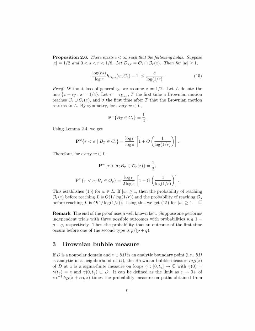
Proposition 2.6. There exists c < ∞ such that the following holds. Suppose|z| = 1/2 and 0 < s < r < 1/8. Let Ds,r = Os ∩ Or(z). Then for |w| ≥ 1,

∣

∣

∣

∣

log(rs)

log rhDs,r(w,Cs) − 1

∣

∣

∣

∣

≤c

log(1/r). (15)

Proof. Without loss of generality, we assume z = 1/2. Let L denote theline {x + iy : x = 1/4}. Let τ = τDs,r , T the first time a Brownian motionreaches Cr ∪ Cr(z), and σ the first time after T that the Brownian motionreturns to L. By symmetry, for every w ∈ L,

Pw{BT ∈ Cr} =1

2.

Using Lemma 2.4, we get

Pw{τ < σ | BT ∈ Cr} =log r

log s

[

1 + O

(

1

log(1/r)

)]

.

Therefore, for every w ∈ L,

Pw{τ < σ;Bτ ∈ Or(z)} =1

2,

Pw{τ < σ;Bτ ∈ Os} =log r

2 log s

[

1 + O

(

1

log(1/r)

)]

.

This establishes (15) for w ∈ L. If |w| ≥ 1, then the probability of reachingOr(z) before reaching L is O(1/ log(1/r)) and the probability of reaching Os

before reaching L is O(1/ log(1/s)). Using this we get (15) for |w| ≥ 1.

Remark The end of the proof uses a well known fact. Suppose one performsindependent trials with three possible outcomes with probabilities p, q, 1 −p − q, respectively. Then the probability that an outcome of the first timeoccurs before one of the second type is p/(p + q).

3 Brownian bubble measure

If D is a nonpolar domain and z ∈ ∂D is an analytic boundary point (i.e., ∂Dis analytic in a neighborhood of D), the Brownian bubble measure mD(z)of D at z is a sigma-finite measure on loops γ : [0, tγ ] → C with γ(0) =γ(tγ) = z and γ(0, tγ) ⊂ D. It can be defined as the limit as ǫ → 0+ ofπ ǫ−1 hD(z + ǫn, z) times the probability measure on paths obtained from

9

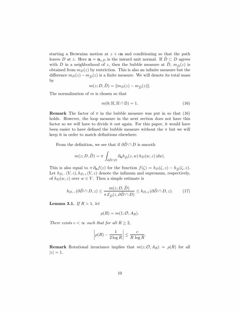
starting a Brownian motion at z + ǫn and conditioning so that the pathleaves D at z. Here n = nz,D is the inward unit normal. If D ⊂ D agreeswith D in a neighborhood of z, then the bubble measure at D, mD(z) isobtained from mD(z) by restriction. This is also an infinite measure but thedifference mD(z)−mD(z) is a finite measure. We will denote its total massby

m(z;D, D) = ‖mD(z) − mD(z)‖.

The normalization of m is chosen so that

m(0; H, H ∩ D) = 1. (16)

Remark The factor of π in the bubble measure was put in so that (16)holds. However, the loop measure in the next section does not have thisfactor so we will have to divide it out again. For this paper, it would havebeen easier to have defined the bubble measure without the π but we willkeep it in order to match definitions elsewhere.

From the definition, we see that if ∂D ∩ D is smooth

m(z;D, D) = π

∫

∂D∩D∂nhD(z,w)hD(w, z) |dw|.

This is also equal to π ∂nf(z) for the function f(ζ) = hD(ζ, z) − hD(ζ, z).Let hD,−(V, z), hD,+(V, z) denote the infimum and supremum, respectively,of hD(w, z) over w ∈ V . Then a simple estimate is

hD,−(∂D ∩ D, z) ≤m(z;D, D)

π ED(z, ∂D ∩ D)≤ hD,+(∂D ∩ D, z). (17)

Lemma 3.1. If R > 1, let

ρ(R) = m(1;O, AR).

There exists c < ∞ such that for all R ≥ 2,

∣

∣

∣

∣

ρ(R) −1

2 log R

∣

∣

∣

∣

≤c

R log R.

Remark Rotational invariance implies that m(z;O, AR) = ρ(R) for all|z| = 1.

10

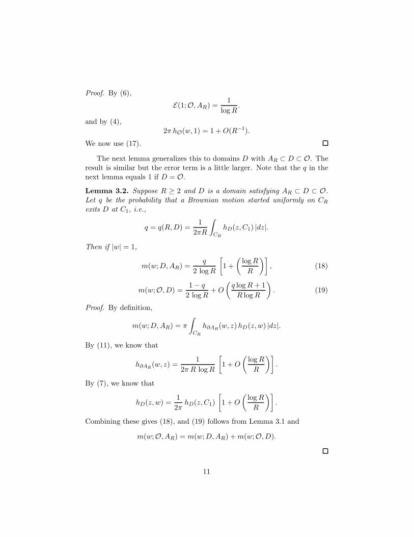
Proof. By (6),

E(1;O, AR) =1

log R.

and by (4),2π hO(w, 1) = 1 + O(R−1).

We now use (17).

The next lemma generalizes this to domains D with AR ⊂ D ⊂ O. Theresult is similar but the error term is a little larger. Note that the q in thenext lemma equals 1 if D = O.

Lemma 3.2. Suppose R ≥ 2 and D is a domain satisfying AR ⊂ D ⊂ O.Let q be the probability that a Brownian motion started uniformly on CR

exits D at C1, i.e.,

q = q(R,D) =1

2πR

∫

CR

hD(z,C1) |dz|.

Then if |w| = 1,

m(w;D,AR) =q

2 log R

[

1 +

(

log R

R

)]

, (18)

m(w;O,D) =1 − q

2 log R+ O

(

q log R + 1

R log R

)

. (19)

Proof. By definition,

m(w;D,AR) = π

∫

CR

h∂AR(w, z)hD(z,w) |dz|.

By (11), we know that

h∂AR(w, z) =

1

2π R log R

[

1 + O

(

log R

R

)]

.

By (7), we know that

hD(z,w) =1

2πhD(z,C1)

[

1 + O

(

log R

R

)]

.

Combining these gives (18), and (19) follows from Lemma 3.1 and

m(w;O, AR) = m(w;D,AR) + m(w;O,D).

11

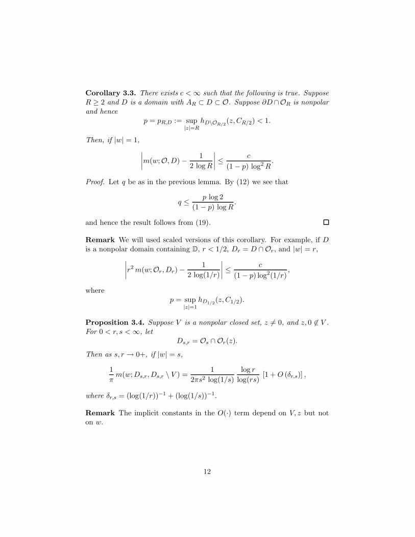
Corollary 3.3. There exists c < ∞ such that the following is true. SupposeR ≥ 2 and D is a domain with AR ⊂ D ⊂ O. Suppose ∂D∩OR is nonpolarand hence

p = pR,D := sup|z|=R

hD\OR/2(z,CR/2) < 1.

Then, if |w| = 1,

∣

∣

∣

∣

m(w;O,D) −1

2 log R

∣

∣

∣

∣

≤c

(1 − p) log2 R.

Proof. Let q be as in the previous lemma. By (12) we see that

q ≤p log 2

(1 − p) log R.

and hence the result follows from (19).

Remark We will used scaled versions of this corollary. For example, if Dis a nonpolar domain containing D, r < 1/2, Dr = D ∩Or, and |w| = r,

∣

∣

∣

∣

r2 m(w;Or,Dr) −1

2 log(1/r)

∣

∣

∣

∣

≤c

(1 − p) log2(1/r),

wherep = sup

|z|=1hD1/2

(z,C1/2).

Proposition 3.4. Suppose V is a nonpolar closed set, z 6= 0, and z, 0 6∈ V .For 0 < r, s < ∞, let

Ds,r = Os ∩ Or(z).

Then as s, r → 0+, if |w| = s,

1

πm(w;Ds,r,Ds,r \ V ) =

1

2πs2 log(1/s)

log r

log(rs)[1 + O (δr,s)] ,

where δr,s = (log(1/r))−1 + (log(1/s))−1.

Remark The implicit constants in the O(·) term depend on V, z but noton w.

12

Proof. We will use (17) and write δ = δr,s. By scaling we may assume z = 2and let d = min{2,dist(0, V ),dist(2, V )}. We will only consider r, s ≤ d/2.By (6),

E(w,Cd;As,d) = s−1 E(w/s,Cd/s;Ad/s) =1

s log(1/s)[1 + O(δ)] .

Using this and (5) we can see that

E(w, V ;Ds,r \ V ) =1

s log(1/s)[1 + O(δ)] .

For ζ ∈ V , (15) gives

hDs,r(ζ, Cs) =log r

log(rs)[1 + O(δ)] . (20)

Therefore. by (7)

hDs,r(ζ, w) =log r

2πs log(rs)[1 + O(δ)] .

The next proposition is the analogue of Proposition 3.4 with z = ∞.

Proposition 3.5. Suppose V is a nonpolar compact set, with 0 6∈ V . For0 < s, r < ∞, let

Ds,r = Os ∩ D1/r.

Then, for as s, r → 0+, if |w| = s,

1

πm(w;Ds,r,Ds,r \ V ) =

1

2πs2 log(1/s)

log r

log(rs)[1 + O (δr,s)] ,

where δr,s = (log(1/r))−1 + (log(1/s))−1.

Proof. The proof is the same as the previous proposition. In fact, it is slighlyeasier because (20) is justified by (5).

13

4 Brownian loop measure

The Brownian loop measure is a measure on unrooted loops. It is thismeasure that is conformally invariant. For computational purposes it isuseful to write the measure in terms of the bubble measure. The followingexpression is obtained by assigning to each unrooted loop the root closestto the origin, see [2].

µ = µC =1

π

∫ 2π

0

∫ ∞

0mOr(re

iθ) r dr dθ. (21)

To be precise, we are considering the right hand side as a measure on un-rooted loops. If D is a subdomain, then µD is defined by restriction. IfDr ⊂ D, then the Brownian loop measure in D restricted to loops thatintersect Dr can be written as

1

π

∫ 2π

0

∫ r

0mDs(se

iθ) s dr dθ, (22)

where Ds = D ∩ Os. If r1 < r, then the Brownian loop measure of loops inOr1

that intersect Dr is given by

1

π

∫ 2π

0

∫ r

r1

mDs(seiθ) s dr dθ.

Using this and appropriate properties of the bubble measure we can concludethe following.

Lemma 4.1. For every 0 < s < r < ∞ and d > 0, the loop measure of theset of loops in Os of diameter at least d that intersect Dr is finite.

Remark This result is not true for s = 0. The Brownian loop measure ofloops in C of diameter greater than d that intersect the unit disk is infinite.See, e.g., Lemma 4.3 below.

Conformal invariance implies that the Brownian loop measure of loopsin Ar,2r that separate the origin from infinity is the the same for all r. It iseasy to see that this measure is positive and the last lemma shows that itis finite. It follows that the measure of the set of loops that surround theorigin is infinite.

If V1, V2, . . . are closed subsets of the Riemann sphere and D is a nonpolardomain, then

Λ(V1, V2, . . . , Vk;D)

14

is defined to be the loop measure of the set of loops in D that intersect allof V1, . . . , Vk. Note that

Λ(V1, V2, . . . , Vk;D) =

Λ(V1, V2, . . . , Vk+1;D) + Λ(V1, V2, . . . , Vk;D \ Vk+1). (23)

If V1, V2, . . . , Vk are the traces of simple curves that include the origin, thenthe comment in the last paragraph shows that for all r > 0,

Λ(V1, V2, . . . , Vk; Dr) = ∞.

Lemma 4.2. Suppose V1, V2 are closed sets and D is a domain. Let

V j = Aej−1,ej , Oj = Oej , Dj = D ∩ Oj.

Then

Λ(V1, V2;D) =

∞∑

j=−∞

Λ(V1, V2, Vj+1;Dj). (24)

Proof. For each unrooted loop, consider the point on the loop closest to theorigin. The measure of the set of loops for which the distance to the originis exactly ej for some integer j is 0. For each loop, there is a unique j suchthat the loop is in Oj but not in Oj+1. Except for a set of loops of measurezero, such a loop intersects V j+1 but does not intersect V k for k < j+1, andhence each loop is counted exactly once on the right-hand side of (24).

Lemma 4.3. There exists c < ∞ such that if 0 < s < 1, R ≥ 2,∣

∣

∣

∣

Λ(C1, CR;Os) − log

[

log(R/s)

log R

]∣

∣

∣

∣

≤c

R log R.

In particular, there exists c < ∞ such that if R ≥ 2/s > 2,

∣

∣

∣

∣

Λ(C1, CR;Os) −log(1/s)

log R

∣

∣

∣

∣

≤c log2(1/s)

log2 R.

Proof. By (22), rotational invariance, and the scaling rule, we get

Λ(C1, CR;Os) = 2

∫ 1

sr m(r;Or, Ar,R) dr = 2

∫ 1

sr−1 ρ(R/r) dr,

where ρ is as in Lemma 3.1. From that lemma, we know that

ρ(R/r) =1

2 log(R/r)+ O

(

r

R log(R/r)

)

,

15

and hence

Λ(C1, CR;Os) = O

(

1

R log R

)

+

∫ 1

s

1

r (log R − log r)dr.

The first assertion follows by integrating and the second from the expansion

log

[

log(R/s)

log R

]

=log(1/s)

log R+ O

(

log2(1/s)

log2 R

)

.

Lemma 4.4. Suppose V is a closed, nonpolar set with 0 6∈ V and α > 0.There exists c = cV,α < ∞ such that for r < min{1,dist(0, V )}/4,

∣

∣

∣

∣

Λ(V,Oαr \ Or;Or) −log α

log(1/r)

∣

∣

∣

∣

≤c

log2(1/r).

Proof. By scaling, we may assume that dist(0, V ) = 1. It suffices to provethe result for r sufficiently small. By (22), we have

Λ(V,Oαr \ Or;Or) =1

π

∫ 2π

0

∫ αr

rm(seiθ;Os,Ds) s ds dr,

where Ds = Os \ V . By Corollary 3.3, for r ≤ s ≤ αr,

m(seiθ;Os,Ds) =1

2s2 log(1/s)

[

1 + O

(

1

log(1/r)

)]

.

Therefore,

Λ(V,Oαr \ Or;Or) =

[

1 + O

(

1

log(1/r)

)]∫ αr

r

ds

s log(1/s).

Also,

∫ αr

r

ds

s log(1/s)= log log

(

1

r

)

− log log

(

1

αr

)

=log α

log(1/r)+ O

(

1

log2(1/r)

)

.

16

Lemma 4.5. Suppose V1, V2 are disjoint, nonpolar closed subsets of theRiemann sphere with 0 6∈ V1. Then there exists c = cV1,V2

< ∞ such thatfor all r ≤ dist(0, V1)/2,

Λ(V1, Cr; C \ V2) ≤c

log(1/r). (25)

Proof. Constants in this proof depend on V1, V2. Without loss of generalityassume 0 6∈ V2 and let Dr = Or \ V2. We will first prove the result forr ≤ r0 = [dist(0, V1) ∧ dist(0, V2)]/2. By (22), we have

Λ(V1, Cr; C \ V2) =1

π

∫

|z|≤rm(z;D|z|,D|z| \ V1) dA(z). (26)

By (14),

hDr(w, z) ≤c

r log(1/r), w ∈ V1, |z| = r.

By comparison with an annulus, we get

ED|z|\V1(z, V1) ≤

c

|z| log(1/|z|), |z| = r.

Using (17), we then have

1

πm(z;D|z|,D|z| \ V1) ≤

c

|z|2 log2(1/|z|).

By integrating, we get (25) for r ≤ r0.Let r1 = dist(0, V1)/2 and note that

Λ(V1, Cr1; C \ V2) ≤ Λ(V1, Cr0

; C \ V2) + Λ(V1, Cr1;Or0

\ V2).

Using Lemma 4.1 we can see that

Λ(V1, Cr1;Or0

\ V2) < ∞.

Therefore,Λ(V1, Cr1

; C \ V2) < ∞,

and we can conclude (25) for r0 ≤ r ≤ r1 with a different constant.

Corollary 4.6. Suppose V1, V2 are disjoint closed subsets of the Riemannsphere and D is a nonpolar domain. Then

Λ(V1, V2;D) < ∞.

17

Proof. Assume 0 6∈ V1. Lemma 4.5 shows that Λ(V1, Ds;D) < ∞ for somes > 0. Note that

Λ(V1, V2;D) ≤ Λ(V1, Ds;D) + Λ(V1, V2;Os).

Since at least one of V1, V2 is compact, Lemma 4.1 implies that

Λ(V1, V2;Os) < ∞.

Theorem 4.7. Suppose V1, V2 are disjoint, nonpolar closed subsets of theRiemann sphere. Then the limit

Λ∗(V1, V2) = limr→0+

[Λ(V1, V2;Or) − log log(1/r)] (27)

exists.

Proof. Without loss of generality, assume that dist(0, V1) ≥ 2 and let Ok =Oe−k . Let V2 ⊂ V2 be a nonpolar closed subset with 0 6∈ V2. Constants inthe proof depend on V1, V2. Since Λ(V1, V2;Or) increases as r decreases to0, it suffices to establish the limit

limk→∞

[

Λ(V1, V2;Ok) − log k

]

.

Repeated application of (23) shows that if k ≥ 1,

Λ(V1, V2;Ok) = Λ(V1, V2;O

0) +k

∑

j=1

Λ(V1, V2,Oj−1 \ Oj;Oj).

Similarly, for fixed k, (23) implies

Λ(V1,Ok−1 \ Ok;Ok) − Λ(V1, V2,O

k−1 \ Ok;Ok)

= Λ(V1,Ok−1 \ Ok;Ok \ V2)

≤ Λ(V1,Ok−1 \ Ok;Ok \ V2).

From Lemma 4.4, we can see that

Λ(V1,Ok−1 \ Ok;Ok) =

1

k+ O

(

1

k2

)

,

18

and hence the limit

limk→∞

− log k +k

∑

j=1

Λ(V1,Ok−1 \ Ok;Ok)

exists and is finite. By Lemma 4.5, we see that

∞∑

j=k

Λ(V1,Oj−1 \ Oj ;Oj \ V2) = Λ(V1, D

k;D \ V2) ≤

c

k,

and hence

∞∑

j=k

[

Λ(V1,Oj−1 \ Oj;Oj) − Λ(V1, V2,O

j−1 \ Oj ;Oj)]

≤c

k,

where the constant c depends on V1 and V2 but not otherwise on V2.

Remark It follows from the proof that

Λ∗(V1, V2) = Λ(V1, V2;Ok) − log k + O

(

1

k

)

,

where the O(·) terms depends on V1 and V2 but not otherwise on V2. As aconsequence we can see that if 0 6∈ V1 and V2,r = V2 ∩ {|z| ≥ r}, then

limr→0+

Λ∗(V1, V2,r) = Λ∗(V1, V2). (28)

The definition of Λ∗ in (27) seems to make the origin a special point.Theorem 4.11 shows that this is not the case.

Lemma 4.8. Suppose V is a nonpolar closed subset, z 6= 0 and 0 6∈ V . Letα > 0. There exists c, r0 (depending on z, V, α) such that if 0 < r < r0,

|Λ(V, C \ Or;Oαr(z)) − log 2| ≤c

log(1/r).

Proof. We will first assume z 6∈ V . For s ≤ r, let Ds = Os ∩ Oαr(z). As in(22),

Λ(V, C \ Or;Oαr(z)) =1

π

∫

|w|≤rm(w;D|w|,D|w| \ V ) dA(w).

19

By Lemma 3.4, if |w| = s ≤ r,

1

πm(w;Ds,Ds \ V ) =

1

2πs2 log(1/s)

log r

log(rs)

[

1 + O

(

1

log(1/r)

)]

,

and therefore,

Λ(V, C \ Or;Oαr(z)) = log r

∫ r

0

ds

s log(1/s) log(rs)

[

1 + O

(

1

log(1/r)

)]

.

A straightforward computation gives

log r

∫ r

0

ds

s log(1/s) log(rs)= log 2.

This finishes the proof for z 6∈ V .If z ∈ V and t > 0, let V1 ⊂ V be a closed nonpolar set with z 6∈ V1.

Then (23) implies

Λ(V, C \ Or;Oαr(z)) =

Λ(V1, C \ Or;Oαr(z)) + Λ(V \ V1, C \ Or;Oαr(z) \ V1).

Since the previous paragraph applies to V1 it suffices to show that

Λ(V \ V1, C \ Or;Oαr(z) \ V1) = O

(

1

log(1/r)

)

.

We can write

Λ(V \ V1, C \ Or;Oαr(z) \ V1) =1

π

∫

|w|≤rm(w;Ds \ V1,Ds \ V ) dA(w).

By using (18) we can see that

m(w;Ds \ V1,Ds \ V ) ≤c

log2(1/s),

and hence

Λ(V \ V1, C \ Or;Oαr(z) \ V1) ≤ c

∫ r

0

ds

s log2(1/s)≤

c

log(1/r).

The following is the equivalent lemma for z = ∞. It can be provedsimilarly or by conformal transforamtion.

20

Lemma 4.9. Suppose V is a nonpolar closed subset, and 0 6∈ V . Let α > 0.There exists c, r0 (depending on V, α) such that if 0 < r < r0,

∣

∣Λ(V, C \ Or; Dα/r) − log 2∣

∣ ≤c

log(1/r).

We extend this to k closed sets.

Lemma 4.10. Suppose V1, . . . , Vk are closed nonpolar subsets of C \ {0}.Let α > 0. There exists c, r0 (depending on z, α, V1, . . . , Vk) such that if0 < r < r0,

|Λ(V1, . . . , Vk, C \ Or;Oαr(z)) − log 2| ≤c

log(1/r).

∣

∣Λ(V1, . . . , Vk, C \ Or; Dα/r) − log 2∣

∣ ≤c

log(1/r).

Proof. If k = 2, inclusion-exclusion implies

Λ(V1 ∪ V2, C \ Or;Oαr(z)) + Λ(V1, V2, , C \ Or;Oαr(z)) =

Λ(V1, C \ Or;Oαr(z)) + Λ(V2, , C \ Or;Oαr(z)).

Since Lemma 4.8 applies to V1 ∪ V2, V1, V2, we get the result. The casesk > 2 and z = ∞ are done similarly.

Theorem 4.11. Suppose V1, V2 are disjoint, nonpolar closed subsets of theRiemann sphere and z ∈ C. Then

Λ∗(V1, V2) = limr→0+

[Λ(V1, V2;Or(z)) − log log(1/r)] .

Moreover,Λ∗(V1, V2) = lim

R→∞[Λ(V1, V2;DR) − log log R] .

Proof. We will assume 0 6∈ V1. Using (27), we see that it suffices to provethat

limr→0+

[Λ(V1, V2;Or(z)) − Λ(V1, V2;Or)] = 0.

Note that

Λ(V1, V2;Or(z)) − Λ(V1, V2;Or) =

Λ(V1, V2, C \ Or;Or(z)) − Λ(V1, V2, C \ Or(z);Or).

21

Lemma 4.10 implies

Λ(V1, V2, C \ Or;Or(z)) = log 2 + O

(

1

log(1/r)

)

, (29)

where the constants in the error term depend on z, V1, V2. Similarly, usingtranslation invariance of the loop measure, we can see that

Λ(V1, V2, C \ Or(z);Or) = log 2 + O

(

1

log(1/r)

)

.

If V1, V2, . . . , Vk are pairwise disjoint nonpolar closed sets of the Riemannsphere, we define similarly

Λ∗(V1, . . . , Vk) = limr→0+

[Λ(V1, V2, . . . , Vk;Or) − log log(1/r)] .

One can prove the existence of the limit in the same way or we can use therelation

Λ∗(V1, . . . , Vk) = Λ∗(V1, . . . , Vk+1) + Λ(V1, . . . , Vk; C \ Vk+1).

References

[1] G. Lawler (2005). Conformally Invariant Processes in the Plane, Amer.Math. Soc.

[2] G. Lawler, Partition functions, loop measure, and versions of SLE, toappear in J. Stat. Phys.

[3] G. Lawler, O. Schramm, W. Werner (2003), Conformal restriction: thechordal case, J. Amer. Math. Soc. 16, 917–955.

[4] G. Lawler, W. Werner (2004), The Brownian loop soup, Probab. TheoryRelated Fields 128, 565–588.

22