Embed Size (px)
Citation preview
MPRAMunich Personal RePEc Archive
A note on matrix differentiation
Pawel Kowal
December 2006
Online at http://mpra.ub.uni-muenchen.de/3917/MPRA Paper No. 3917, posted 9. July 2007
A note on matrix differentiation
Paweł Kowal
July 9, 2007
Abstract
This paper presents a set of rules for matrix differentiation withrespect to a vector of parameters, using the flattered representation ofderivatives, i.e. in form of a matrix. We also introduce a new set ofKronecker tensor products of matrices. Finally we consider a problemof differentiating matrix determinant, trace and inverse.
JEL classification: C00
Keywords: matrix differentiation, generalized Kronecker products
1 IntroductionDerivatives of matrices with respect to a vector of parameters can be ex-
pressed as a concatenation of derivatives with respect to a scalar parameters.However such a representation of derivatives is very inconvenient in someapplications, e.g. if higher order derivatives are considered, and or even arenot applicable if matrix functions (like determinant or inverse) are present.For example finding an explicit derivative of det(∂X/∂θ) would be a quitecomplicated task. Such a problem arise naturally in many applications, e.g.in maximum likelihood approach for estimating model parameters.
The same problems emerges in case of a tensor representation of deriva-tives. Additionally, in this case additional effort is required to find the flat-tered representation of resulting tensors, which is required, since runningnumerical computations efficiently is possible only in case of two dimensionaldata structures.
In this paper we derive formulas for differentiating matrices with respectto a vector of parameters, when one requires the flattered form of resultingderivatives, i.e. representation of derivatives in form of matrices. To do this
we introduce a new set of the Kronecker matrix products as well as the gener-alized matrix transposition. Then, first order and higher order derivatives offunctions being compositions of primitive function using elementary matrixoperations like summation, multiplication, transposition and the Kroneckerproduct, can be expressed in a closed form based on primitive matrix func-tions and their derivatives, using these elementary operations, the generalizedKronecker products and the generalized transpositions.
We consider also more general matrix functions containing matrix func-tions (inverse, trace and determinant). Defining the generalized trace func-tion we are able to express derivatives of such functions in closed form.
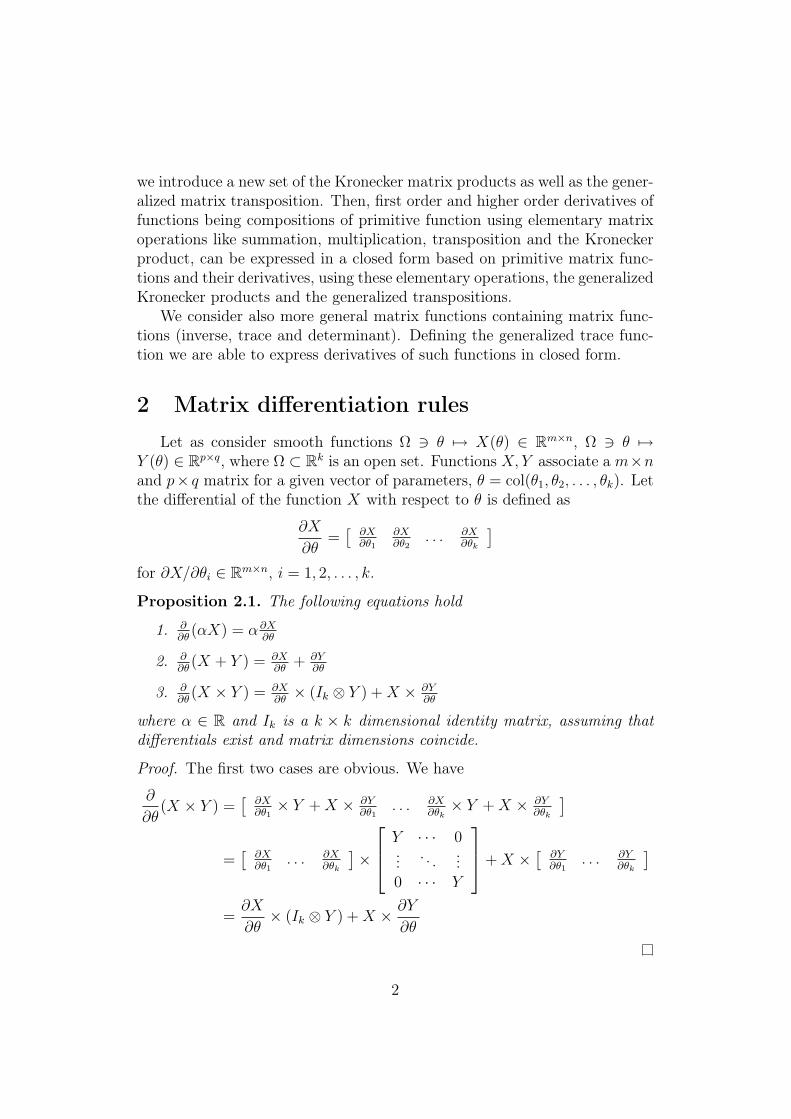
2 Matrix differentiation rulesLet as consider smooth functions Ω 3 θ 7→ X(θ) ∈ Rm×n, Ω 3 θ 7→
Y (θ) ∈ Rp×q, where Ω ⊂ Rk is an open set. Functions X,Y associate a m×nand p× q matrix for a given vector of parameters, θ = col(θ1, θ2, . . . , θk). Letthe differential of the function X with respect to θ is defined as
∂X
∂θ=
[∂X∂θ1
∂X∂θ2
. . . ∂X∂θk
]
for ∂X/∂θi ∈ Rm×n, i = 1, 2, . . . , k.
Proposition 2.1. The following equations hold
1. ∂∂θ
(αX) = α∂X∂θ
2. ∂∂θ
(X + Y ) = ∂X∂θ
+ ∂Y∂θ
3. ∂∂θ
(X × Y ) = ∂X∂θ× (Ik ⊗ Y ) + X × ∂Y
∂θ
where α ∈ R and Ik is a k × k dimensional identity matrix, assuming thatdifferentials exist and matrix dimensions coincide.
Proof. The first two cases are obvious. We have
∂
∂θ(X × Y ) =
[∂X∂θ1
× Y + X × ∂Y∂θ1
. . . ∂X∂θk
× Y + X × ∂Y∂θk
]
=[
∂X∂θ1
. . . ∂X∂θk
]×
Y · · · 0... . . . ...0 · · · Y
+ X × [
∂Y∂θ1
. . . ∂Y∂θk
]
=∂X
∂θ× (Ik ⊗ Y ) + X × ∂Y
∂θ
2

Differentiating matrix transposition is a little bit more complicated. Letus define a generalized matrix transposition
Definition 2.2. Let X = [X1, X2, . . . Xn], where Xi ∈ Rp×q, i = 1, 2, . . . , nis a p× q matrix is a partition of p× nq dimensional matrix X. Then
Tn(X).=
[X ′
1, X′2, . . . , X
′n
]
Proposition 2.3. The following equations hold
1. ∂∂θ
(X ′) = Tk(∂X∂θ
)
2. ∂∂θ
(Tn(X)) = Tk×n(∂X∂θ
)
Proof. The first condition is a special case of the second condition for n = 1.We have
∂
∂θ(T(n)(X)) =
[T(n)(
∂X∂θ1
) . . . T(n)(∂X∂θk
)]
=[
∂X′1
∂θ1, . . . , ∂X′
n
∂θ1. . .
∂X′1
∂θk, . . . , ∂X′
n
∂θk
]= T(k×n)
(∂X
∂θ
)
since∂X
∂θ=
[∂X1
∂θ1, . . . , ∂Xn
∂θ1. . . ∂X1
∂θk, . . . , ∂Xn
∂θk
]
Let us now turn to differentiating tensor products of matrices. Let forany matrices X, Y , where X ∈ Rp×q is a matrix with elements xij ∈ R fori = 1, 2, . . . , p, j = 1, 2, . . . , q. The Kronecker product, X ⊗ Y is defined as
X ⊗ Y.=
x11Y · · · x1qY... . . . ...
xp1Y · · · xpqY
Similarly as in case of differentiating matrix transposition we need to intro-duce the generalized Kronecker product
Definition 2.4. Let X = [X1, X2, . . . Xm], where Xi ∈ Rp×q, i = 1, 2, . . . , mis a p × q matrix is a partition of p ×mq dimensional matrix X. Let Y =[Y1, Y2, . . . Yn], where Yi ∈ Rr×s, i = 1, 2, . . . , n is a r×s matrix is a partitionof r × ns dimensional matrix Y . Then
X ⊗1n Y
.= [X ⊗ Y1, . . . , X ⊗ Yn]
X ⊗mn Y
.= [X1 ⊗1
n Y, . . . , Xm ⊗1n Y ]
X ⊗1,m2,...,msn1,n2,...,ns
Y.= [X ⊗m2,...,ms
n2,...,nsY1, . . . , X ⊗m2,...,ms
n2,...,nsYn1 ]
X ⊗m1,m2,...,msn1,n2,...,ns
Y.= [X1 ⊗1,m2,...,ms
n1,n2,...,nsY, . . . , Xm1 ⊗1,m2,...,ms
n1,n2,...,nsY ]
assuming that appropriate matrix partitions exist.
3

Proposition 2.5. The following equations hold
1. ∂∂θ
(X ⊗ Y ) = ∂X∂θ⊗ Y + X ⊗1
k∂Y∂θ
2. ∂∂θ
(X ⊗m1,...,msn1,...,ns
Y ) = ∂X∂θ⊗k,m1,...,ms
1,n1,...,nsY + X ⊗1,m1,...,ms
k,n1,...,ns
∂Y∂θ
Proof. We have
∂
∂θ(X ⊗m1,...,ms
n1,...,nsY ) =
[∂
∂θ1(X ⊗m1,...,ms
n1,...,nsY ) · · · ∂
∂θk(X ⊗m1,...,ms
n1,...,nsY )
]
=[
∂X∂θ1
⊗m1,...,msn1,...,ns
Y · · · ∂X∂θk
⊗m1,...,msn1,...,ns
Y]
+[
X ⊗m1,...,msn1,...,ns
∂Y∂θ1
· · · X ⊗m1,...,msn1,...,ns
∂Y∂θk
]
=∂X
∂θ⊗k,m1,...,ms
1,n1,...,nsY + X ⊗1,m1,...,ms
k,n1,...,ns
∂Y
∂θ
Since X⊗Y = X⊗11 Y , in case of the standard Kronecker product we obtain
∂
∂θ(X ⊗ Y ) =
∂X
∂θ⊗k
1 Y + X ⊗1k
∂Y
∂θ=
∂X
∂θ⊗ Y + X ⊗1
k
∂Y
∂θ
In proposition 2.1 we have omitted the case of multiplication of a matrixby a scalar function, using proposition 2.5 we obtain
Proposition 2.6. Let α is a scalar function of θ and X is a matrix valuedfunction of θ, X(θ) ∈ Rp×q. Then
∂
∂θ(αX) = α× ∂X
∂θ+
∂α
∂θ⊗X
Proof. Expression αX can be represented as αX = (α ⊗ Ip) × X, where Ip
is a p× p dimensional identity matrix. Hence
∂
∂θ(αX) =
∂
∂θ((α⊗ Ip)×X) =
∂(α⊗ Ip)
∂θ× (Ik ⊗X) + (α⊗ Ip)× ∂X
∂θ
= (∂α
∂θ⊗ Ip)× (Ik ⊗X) + α× ∂X
∂θ=
∂α
∂θ⊗X + α× ∂X
∂θ
Let S is a set of smooth matrix valued functions Ω 3 θ 7→ X(θ) ∈ Rp×q,where Ω ⊂ Rk is an open set, for any integers p, q ≥ 1 not necessary the samefor all functions in S. Let dif S .
= ∂X/∂θ : X ∈ S. The set S may containscalars and matrices, which are interpreted as constant functions.
4
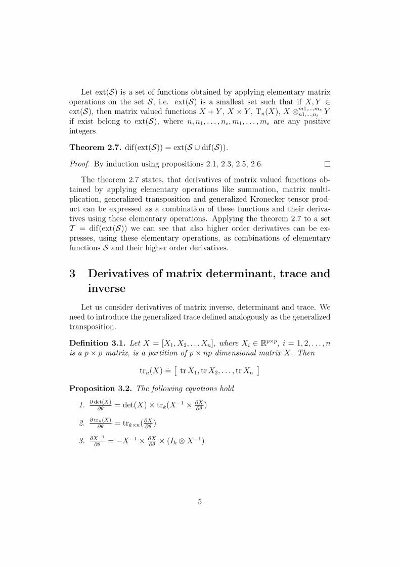
Let ext(S) is a set of functions obtained by applying elementary matrixoperations on the set S, i.e. ext(S) is a smallest set such that if X,Y ∈ext(S), then matrix valued functions X + Y , X × Y , Tn(X), X ⊗m1,...,ms
n1,...,nsY
if exist belong to ext(S), where n, n1, . . . , ns,m1, . . . , ms are any positiveintegers.
Theorem 2.7. dif(ext(S)) = ext(S ∪ dif(S)).
Proof. By induction using propositions 2.1, 2.3, 2.5, 2.6.
The theorem 2.7 states, that derivatives of matrix valued functions ob-tained by applying elementary operations like summation, matrix multi-plication, generalized transposition and generalized Kronecker tensor prod-uct can be expressed as a combination of these functions and their deriva-tives using these elementary operations. Applying the theorem 2.7 to a setT = dif(ext(S)) we can see that also higher order derivatives can be ex-presses, using these elementary operations, as combinations of elementaryfunctions S and their higher order derivatives.
3 Derivatives of matrix determinant, trace andinverse
Let us consider derivatives of matrix inverse, determinant and trace. Weneed to introduce the generalized trace defined analogously as the generalizedtransposition.
Definition 3.1. Let X = [X1, X2, . . . Xn], where Xi ∈ Rp×p, i = 1, 2, . . . , nis a p× p matrix, is a partition of p× np dimensional matrix X. Then
trn(X).=
[tr X1, tr X2, . . . , tr Xn
]
Proposition 3.2. The following equations hold
1. ∂ det(X)∂θ
= det(X)× trk(X−1 × ∂X
∂θ)
2. ∂ trn(X)∂θ
= trk×n(∂X∂θ
)
3. ∂X−1
∂θ= −X−1 × ∂X
∂θ× (Ik ⊗X−1)
5
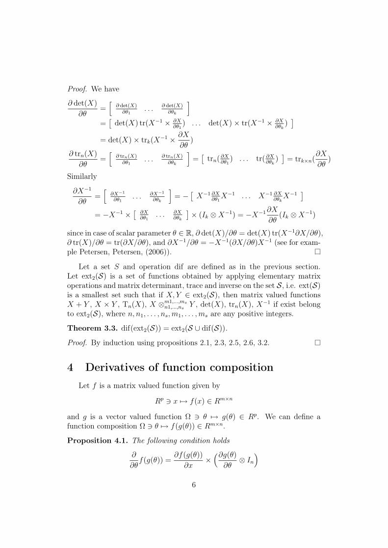
Proof. We have
∂ det(X)
∂θ=
[∂ det(X)
∂θ1. . . ∂ det(X)
∂θk
]
=[
det(X) tr(X−1 × ∂X∂θ1
) . . . det(X)× tr(X−1 × ∂X∂θk
)]
= det(X)× trk(X−1 × ∂X
∂θ)
∂ trn(X)
∂θ=
[∂ trn(X)
∂θ1. . . ∂ trn(X)
∂θk
]=
[trn( ∂X
∂θ1) . . . tr( ∂X
∂θk)
]= trk×n(
∂X
∂θ)
Similarly
∂X−1
∂θ=
[∂X−1
∂θ1. . . ∂X−1
∂θk
]= − [
X−1 ∂X∂θ1
X−1 . . . X−1 ∂X∂θk
X−1]
= −X−1 × [∂X∂θ1
. . . ∂X∂θk
]× (Ik ⊗X−1) = −X−1∂X
∂θ(Ik ⊗X−1)
since in case of scalar parameter θ ∈ R, ∂ det(X)/∂θ = det(X) tr(X−1∂X/∂θ),∂ tr(X)/∂θ = tr(∂X/∂θ), and ∂X−1/∂θ = −X−1(∂X/∂θ)X−1 (see for exam-ple Petersen, Petersen, (2006)).
Let a set S and operation dif are defined as in the previous section.Let ext2(S) is a set of functions obtained by applying elementary matrixoperations and matrix determinant, trace and inverse on the set S, i.e. ext(S)is a smallest set such that if X,Y ∈ ext2(S), then matrix valued functionsX + Y , X × Y , Tn(X), X ⊗m1,...,ms
n1,...,nsY , det(X), trn(X), X−1 if exist belong
to ext2(S), where n, n1, . . . , ns,m1, . . . , ms are any positive integers.
Theorem 3.3. dif(ext2(S)) = ext2(S ∪ dif(S)).
Proof. By induction using propositions 2.1, 2.3, 2.5, 2.6, 3.2.
4 Derivatives of function compositionLet f is a matrix valued function given by
Rp 3 x 7→ f(x) ∈ Rm×n
and g is a vector valued function Ω 3 θ 7→ g(θ) ∈ Rp. We can define afunction composition Ω 3 θ 7→ f(g(θ)) ∈ Rm×n.
Proposition 4.1. The following condition holds
∂
∂θf(g(θ)) =
∂f(g(θ))
∂x×
(∂g(θ)
∂θ⊗ In
)
6
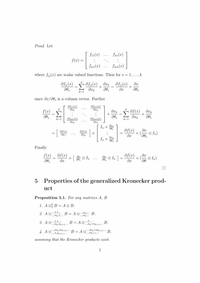
Proof. Let
f(x) =
f11(x) . . . f1n(x)... . . . ...
fm1(x) . . . fmn(x)
where fij(x) are scalar valued functions. Then for s = 1, . . . , k
∂fij(x)
∂θs
=
p∑
k=1
∂fij(x)
∂xk
× ∂xk
∂θs
=∂fij(x)
∂x× ∂x
∂θs
since ∂x/∂θs is a column vector. Further
f(x)
∂θs
=
p∑
k=1
∂f11(x)∂xk
. . . ∂f1n(x)∂xk... . . . ...
∂fm1(x)∂xk
. . . ∂fmn(x)∂xk
× ∂xk
∂θs
=
p∑
k=1
∂f(x)
∂xk
× ∂xk
∂θs
=[
∂f(x)∂x1
. . . ∂f(x)∂xp
]×
In × ∂x1
∂θs...In × ∂xp
∂θs
=
∂f(x)
∂x× (
∂x
∂θs
⊗ In)
Finally
f(x)
∂θs
=∂f(x)
∂x× [
∂x∂θ1
⊗ In . . . ∂x∂θk
⊗ In
]=
∂f(x)
∂x× (
∂x
∂θ⊗ In)
5 Properties of the generalized Kronecker prod-uct
Proposition 5.1. For any matrices A, B
1. A⊗k1 B = A⊗B.
2. A⊗...,1,1,......,nk,1,... B = A⊗...,mk,...
...,nk,... B.
3. A⊗...,1,1,......,nk,nk+1,... B = A⊗...,1,...
...,nk×nk+1,... B.
4. A⊗...,mk,mk+1,......,1,nk+1,... B = A⊗...,mk×mk+1,...
...,nk+1,... B.
assuming that the Kronecker products exist.
7

Proposition 5.2. For any matrices A, B, C
1. A⊗m1,...,mkn1,...,nk
(B + C) = A⊗m1,...,mkn1,...,nk
B + A⊗m1,...,mkn1,...,nk
C.
2. (A + B)⊗m1,...,mkn1,...,nk
C = A⊗m1,...,mkn1,...,nk
C + B ⊗m1,...,mkn1,...,nk
C.
assuming that the Kronecker products exist and matrix dimensions coincide.
Proposition 5.3. For any matrices A, B, C, D
(AB)⊗m1,...,msn1,...,ns
(CD) = (A⊗ C)× (B ⊗m1,...,msn1,...,ns
D)
assuming that products AB and CD, as well as Kronecker products exist.
Proof. Observe that X ⊗m1,...,msn1,...,ns
Y = X ⊗m1,...,ms,1n1,...,ns,1 Y , and (AB)⊗1
1 (CD) =(A ⊗ C) × (B ⊗1
1 D), since (AB) ⊗ (CD) = (A ⊗ C) × (B ⊗ D). Let(AB)⊗mk,...,m1,1
nk,...,n1,1 (CD) = (A⊗ C)× (B ⊗mk,...,m1,1nk,...,n1,1 D) for k ≥ 0. Then
(AB)⊗1,mk,...,m1,1nk+1,nk,...,n1,1 (CD)
=[
(AB)⊗mk,...,m1,1nk,...,n1,1 (CD1) . . . , (AB)⊗mk,...,m1,1
nk,...,n1,1 (CDnk+1)
]
=[
(A⊗ C)(B ⊗mk,...,m1,1nk,...,n1,1 D1) . . . , (A⊗ C)(B ⊗mk,...,m1,1
nk,...,n1,1 Dnk+1)
]
= (A⊗ C)× (B ⊗1,mk,...,m1,1nk+1,nk,...,n1,1 D)
Similarly
(AB)⊗mk+1,mk,...,m1,1nk+1,nk,...,n1,1 (CD)
=[
(AB1)⊗1,mk,...,m1,1nk+1,nk,...,n1,1 (CD) . . . , (ABmk+1
)⊗1,mk,...,m1,1nk+1,nk,...,n1,1 (CD)
]
=[
(A⊗ C)(B1 ⊗1,mk,...,m1,1nk+1,nk,...,n1,1 D) . . . , (A⊗ C)(Bmk+1
⊗1,mk,...,m1,1nk+1,nk,...,n1,1 D)
]
= (A⊗ C)× (B ⊗mk+1,mk,...,m1,1nk+1,nk,...,n1,1 D)
Proposition 5.4. For any matrices A, B of size p1 × q1 and p2 × q2
A⊗m1,...,msn1,...,ns
B = (A⊗B)× (Iq1 ⊗m1,...,msn1,...,ns
Iq2)
assuming that Kronecker product exists.
Proposition 5.5. For any matrices A, B, C
A⊗m1,...,msn1,...,ns
(B ⊗ C) = (A⊗m1,...,msn1,...,ns
B)⊗ C
assuming that Kronecker products exist.
8
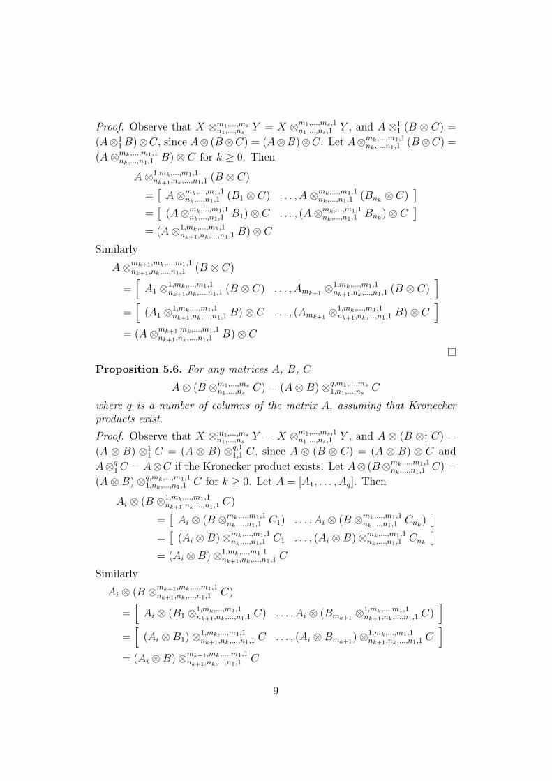
Proof. Observe that X ⊗m1,...,msn1,...,ns
Y = X ⊗m1,...,ms,1n1,...,ns,1 Y , and A ⊗1
1 (B ⊗ C) =
(A⊗11 B)⊗C, since A⊗ (B⊗C) = (A⊗B)⊗C. Let A⊗mk,...,m1,1
nk,...,n1,1 (B⊗C) =
(A⊗mk,...,m1,1nk,...,n1,1 B)⊗ C for k ≥ 0. Then
A⊗1,mk,...,m1,1nk+1,nk,...,n1,1 (B ⊗ C)
=[
A⊗mk,...,m1,1nk,...,n1,1 (B1 ⊗ C) . . . , A⊗mk,...,m1,1
nk,...,n1,1 (Bnk⊗ C)
]
=[
(A⊗mk,...,m1,1nk,...,n1,1 B1)⊗ C . . . , (A⊗mk,...,m1,1
nk,...,n1,1 Bnk)⊗ C
]
= (A⊗1,mk,...,m1,1nk+1,nk,...,n1,1 B)⊗ C
Similarly
A⊗mk+1,mk,...,m1,1nk+1,nk,...,n1,1 (B ⊗ C)
=[
A1 ⊗1,mk,...,m1,1nk+1,nk,...,n1,1 (B ⊗ C) . . . , Amk+1
⊗1,mk,...,m1,1nk+1,nk,...,n1,1 (B ⊗ C)
]
=[
(A1 ⊗1,mk,...,m1,1nk+1,nk,...,n1,1 B)⊗ C . . . , (Amk+1
⊗1,mk,...,m1,1nk+1,nk,...,n1,1 B)⊗ C
]
= (A⊗mk+1,mk,...,m1,1nk+1,nk,...,n1,1 B)⊗ C
Proposition 5.6. For any matrices A, B, C
A⊗ (B ⊗m1,...,msn1,...,ns
C) = (A⊗B)⊗q,m1,...,ms
1,n1,...,nsC
where q is a number of columns of the matrix A, assuming that Kroneckerproducts exist.Proof. Observe that X ⊗m1,...,ms
n1,...,nsY = X ⊗m1,...,ms,1
n1,...,ns,1 Y , and A ⊗ (B ⊗11 C) =
(A ⊗ B) ⊗11 C = (A ⊗ B) ⊗q,1
1,1 C, since A ⊗ (B ⊗ C) = (A ⊗ B) ⊗ C andA⊗q
1 C = A⊗C if the Kronecker product exists. Let A⊗ (B⊗mk,...,m1,1nk,...,n1,1 C) =
(A⊗B)⊗q,mk,...,m1,11,nk,...,n1,1 C for k ≥ 0. Let A = [A1, . . . , Aq]. Then
Ai ⊗ (B ⊗1,mk,...,m1,1nk+1,nk,...,n1,1 C)
=[
Ai ⊗ (B ⊗mk,...,m1,1nk,...,n1,1 C1) . . . , Ai ⊗ (B ⊗mk,...,m1,1
nk,...,n1,1 Cnk)
]
=[
(Ai ⊗B)⊗mk,...,m1,1nk,...,n1,1 C1 . . . , (Ai ⊗B)⊗mk,...,m1,1
nk,...,n1,1 Cnk
]
= (Ai ⊗B)⊗1,mk,...,m1,1nk+1,nk,...,n1,1 C
Similarly
Ai ⊗ (B ⊗mk+1,mk,...,m1,1nk+1,nk,...,n1,1 C)
=[
Ai ⊗ (B1 ⊗1,mk,...,m1,1nk+1,nk,...,n1,1 C) . . . , Ai ⊗ (Bmk+1
⊗1,mk,...,m1,1nk+1,nk,...,n1,1 C)
]
=[
(Ai ⊗B1)⊗1,mk,...,m1,1nk+1,nk,...,n1,1 C . . . , (Ai ⊗Bmk+1
)⊗1,mk,...,m1,1nk+1,nk,...,n1,1 C
]
= (Ai ⊗B)⊗mk+1,mk,...,m1,1nk+1,nk,...,n1,1 C
9

Finally,
A⊗ (B ⊗mk+1,mk,...,m1,1nk+1,nk,...,n1,1 C)
=[
A1 ⊗ (B ⊗mk+1,mk,...,m1,1nk+1,nk,...,n1,1 C) . . . , Aq ⊗ (B ⊗mk+1,mk,...,m1,1
nk+1,nk,...,n1,1 C)]
=[
(A1 ⊗B)⊗mk+1,mk,...,m1,1nk+1,nk,...,n1,1 C) . . . , (Aq ⊗B)⊗mk+1,mk,...,m1,1
nk+1,nk,...,n1,1 C)]
= (A⊗B)⊗q,mk+1,mk,...,m1,11,nk+1,nk,...,n1,1 C
Proposition 5.7. Let A is m× n matrix. Let B is p× q matrix. Then
A⊗1q B = (Im ⊗1
p Ip)× (B ⊗ A)
Proof. Let Ai is i-th column of A and Bj is j-th column of B. Let Ikp denotes
k-th column of p× p identity matrix and let Bij denotes element of B at j-th
row and i-th column. Then
(Im ⊗1p Ip)× (Bj ⊗ Ai) =
[Im ⊗ I1
p . . . Im ⊗ Ipp
]×
Bj1A
i
. . .Bj
pAi
=
p∑r=1
(Im ⊗ Irp)× (Ai ⊗Bj
r) =
p∑r=1
Ai ⊗ (Irp ×Bj
r) = Ai ⊗Bj
Further
(Im ⊗1p Ip)× (Bj ⊗ A) = (Im ⊗1
p Ip)×[
Bj ⊗ A1 . . . Bj ⊗ An]
=[
A1 ⊗Bj . . . An ⊗Bj]
= A⊗Bj
(Im ⊗1p Ip)× (B ⊗ A) = (Im ⊗1
p Ip)×[
B1 ⊗ A . . . Bq ⊗ A]
=[
A⊗B1 . . . A⊗Bq]
= A⊗1q B
Proposition 5.8. Let A is m× n matrix. Let B is p× q matrix. Then
A⊗1,n1,...,1,ns,1m1,1,...,ms,1,q/m B = (Im ⊗1
p Ip)× (B ⊗m1,...,msn1,...,ns
A)
where m = m1 × · · · ×ms, assuming that the Kronecker products exist.
10
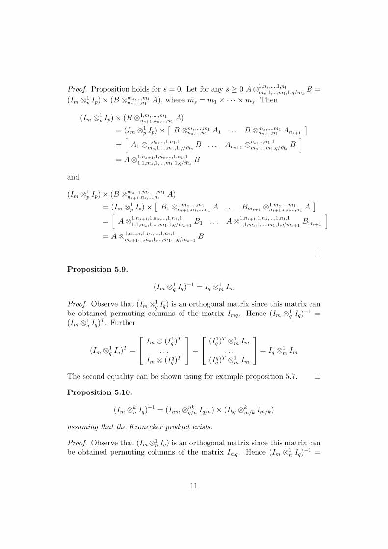
Proof. Proposition holds for s = 0. Let for any s ≥ 0 A⊗1,ns,...,1,n1
ms,1,...,m1,1,q/msB =
(Im ⊗1p Ip)× (B ⊗ms,...,m1
ns,...,n1A), where ms = m1 × · · · ×ms. Then
(Im ⊗1p Ip)× (B ⊗1,ms,...,m1
ns+1,ns,...,n1A)
= (Im ⊗1p Ip)×
[B ⊗ms,...,m1
ns,...,n1A1 . . . B ⊗ms,...,m1
ns,...,n1Ans+1
]
=[
A1 ⊗1,ns,...,1,n1,1ms,1,...,m1,1,q/ms
B . . . Ans+1 ⊗ns,...,n1,1ms,...,m1,q/ms
B]
= A⊗1,ns+1,1,ns,...,1,n1,11,1,ms,1,...,m1,1,q/ms
B
and
(Im ⊗1p Ip)× (B ⊗ms+1,ms,...,m1
ns+1,ns,...,n1A)
= (Im ⊗1p Ip)×
[B1 ⊗1,ms,...,m1
ns+1,ns,...,n1A . . . Bms+1 ⊗1,ms,...,m1
ns+1,ns,...,n1A
]
=[
A⊗1,ns+1,1,ns,...,1,n1,11,1,ms,1,...,m1,1,q/ms+1
B1 . . . A⊗1,ns+1,1,ns,...,1,n1,11,1,ms,1,...,m1,1,q/ms+1
Bms+1
]
= A⊗1,ns+1,1,ns,...,1,n1,1ms+1,1,ms,1,...,m1,1,q/ms+1
B
Proposition 5.9.
(Im ⊗1q Iq)
−1 = Iq ⊗1m Im
Proof. Observe that (Im⊗1q Iq) is an orthogonal matrix since this matrix can
be obtained permuting columns of the matrix Imq. Hence (Im ⊗1q Iq)
−1 =(Im ⊗1
q Iq)T . Further
(Im ⊗1q Iq)
T =
Im ⊗ (I1q )T
. . .Im ⊗ (Iq
q )T
=
(I1q )T ⊗1
m Im
. . .(Iq
q )T ⊗1
m Im
= Iq ⊗1
m Im
The second equality can be shown using for example proposition 5.7.
Proposition 5.10.
(Im ⊗kn Iq)
−1 = (Inm ⊗nkq/n Iq/n)× (Ikq ⊗k
m/k Im/k)
assuming that the Kronecker product exists.
Proof. Observe that (Im⊗1n Iq) is an orthogonal matrix since this matrix can
be obtained permuting columns of the matrix Imq. Hence (Im ⊗1n Iq)
−1 =
11
(Im ⊗1n Iq)
T . Further
In ⊗ (Iq/n ⊗1m Im)× (Im ⊗1
n Iq)T =
(Iq/n ⊗1m Im)× Im ⊗ (I1
q )T
. . .(Iq/n ⊗1
m Im)× Im ⊗ (Inq )T
=
(I1q )T ⊗1
m Im
. . .(In
q )T ⊗1m Im
= Iq ⊗1
m Im
The second equality can be shown using for example proposition 5.7. Hence
(Im ⊗1n Iq)
−1 =(In ⊗ (Iq/n ⊗1
m Im)−1)×(Iq ⊗1
m Im)
=(In ⊗ (Im ⊗1
q/n Iq/n))×(Iq ⊗1
m Im)
= (Inm ⊗nq/n Iq/n)× (Iq ⊗1
m Im)
Further(Im ⊗k
n Iq
)−1
=((Ik ⊗ Im/k)⊗k,1
1,n Iq
)−1
=(Ik ⊗ (Im/k ⊗1
n Iq))−1
= Ik ⊗((Inm/k ⊗n
q/n Iq/n)× (Iq ⊗1m/k Im/k)
)
= Ik ⊗ (Inm/k ⊗nq/n Iq/n)× Ik ⊗ (Iq ⊗1
m/k Im/k)
= (Inm ⊗nkq/n Iq/n)× (Ikq ⊗k
m/k Im/k)
Proposition 5.11. Let A is m× n matrix. Let B is p× q matrix. Then
A⊗B = (Im ⊗1p Ip)× (B ⊗ A)× (Iq ⊗1
n In)
Proof.
(Im ⊗1p Ip)× (B ⊗ A) = A⊗1
q B = (A⊗B)× (In ⊗1q Iq)
= (A⊗B)× (Iq ⊗1n In)−1
6 Concluding remarksDerived formulas requires matrix tensor products, which are absent, when
representing derivatives as the concatenation of derivatives with respect to ascalar parameters. Hence, this approach may decrease numerical efficiency.This problem however can be resolved using appropriate data structures.
12

References[1] T.P. Minka. Old and new matrix algebra useful for statistics. notes,
December 2000.
[2] K.P. Petersen and M. S. Petersen. The matrix cookbook. notes, 2006.
13