IEEE TRANSACTIONS ON EDUCATION, VOL. 42, NO. 3, AUGUST 1999 225

Short Papers

A Note on Kalman Filtering

Chiman M. Kwan,Senior Member,

IEEE, and Frank L. Lewis,Fellow, IEEE

Abstract—The purpose of this paper is to point out a confusing phenom-enon in the teaching of Kalman filtering. Students are often confused bynoting that the a posteriorierror covariance of the discrete Kalman filter(DKF) is smaller than the error covariance of the continuous Kalmanfilter (CKF), which would mean that the DKF is better than CKF since itgives a smaller error covariance. However, simulation results show thatCKF gives estimates much closer to the true states. We will provide asimple qualitative argument to explain this phenomenon.

Index Terms—Covariance, Kalman filter, state estimate.

I. INTRODUCTION

Given a continuous state-space system model, there are three waysof Kalman filter design depending upon the measurement process.

1) If the measurement process is continuous, we should use

a) the continuous Kalman filter (CKF).

2) If the measurement process is discrete, one has two options:

a) design a continuous-discrete Kalman filter (CDKF);b) discretize the continuous model and design a discrete

Kalman filter (DKF)

Students often ask the following reasonable question: Which oneis the best? It is obvious that CKF gives the best performance sincethere is a continuous flow of measurement data (information) intothe Kalman filter. Also one should note that the DKF and CDKFconverge to the CKF as the sampling periodT goes to zero. However,when one plots the error covariance of the three designs, he discoversthat, for finiteT , the DKF and CDKF give lowera posteriori errorcovariances which would mean DKF and CDKF are better than CKF(Figs. 1–3). The most confusing thing is that, asT goes larger, thea posteriori error covariances of DKF and CDKF go even smaller.This is completely absurd because the actual estimation error growsup with increasingT !

It should be noted that no textbooks (for example, [1]–[3] andreferences therein) have addressed this issue yet. We believe this isan important issue that is worth discussion.

II. M AIN RESULTS

Consider a very simple continuous system

_x =0:2x+ w

z =x+ v: (1)

We will use the symboln � (n; Pn) to denote a random processn with n, Pn the mean and covariance ofn, respectively. Here

Manuscript received September 15, 1994; revised March 9, 1999.C. M. Kwan is with Intelligent Automation Incorporated, Rockville, MD

20850 USA.F. L. Lewis is with the Automation and Robotics Research Institute, The

University of Texas at Arlington, Fort Worth, TX 76118 USA.Publisher Item Identifier S 0018-9359(99)06324-4.

w � (0; 1) is the process noise,v � (0; 0:5) is the measurementnoise, and the initial conditionx(0) � (0; 1): Note thatw, v, andx(0) are mutually uncorrelated with each other.

Following the procedure of [1], the CKF can be designed asfollows:

_x =0:2x+K(t)(z � x)

_Pc =0:4Pc + 1� 2P 2

c

K(t) = 2Pc (2)

wherePc is the continuous error covariance between the true statex(t) and the estimated statex(t): Suppose the sampling period isT:The discrete model (1) is given by

xk+1 =Asxk + wk; wk � (0;Qs)

zk =xk + vk; vk � (0; Rs) (3)

where

As = e0:2T

Qs =T

0

e0:4t dt = 2:5(e0:4T � 1)

Rs =0:5

T:

Based on (3), we can design a DKF based on the procedure of [1]as follows.

Initialization:

x0 = 0; P0 = 1:

Time update:

xk+1 =0:2xk;

P�k+1 =0:4Pk + 1:

Measurement update attk:

Pk+1 = [(P�k+1)

�1 + (Rs)�1]�1

xk+1 = x�k+1 +Kk+1(zk+1 � x�

k+1)

Kk+1 =Pk+1=Rs: (4)

We can also design a CDKF using the procedures of [1] as follows.Initialization:

x0 = 0; P0 = 1:

Time update:

_x =0:2x;

_Pcd =0:4Pcd + 1:

Measurement update at timestk:

Kk =P�(tk)[P�(tk) +Rs]�1

P (tk) = (I �Kk)P�(tk)

xk = x�k+Kk(zk � x�

k): (5)

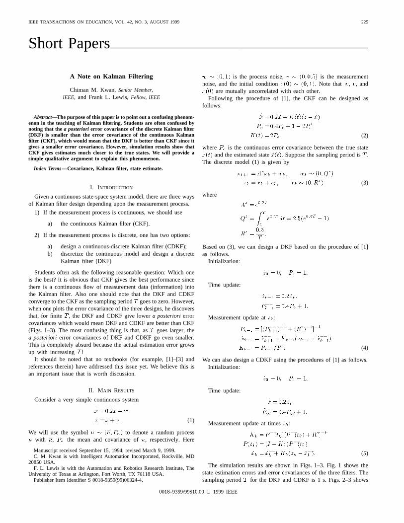
The simulation results are shown in Figs. 1–3. Fig. 1 shows thestate estimation errors and error covariances of the three filters. Thesampling periodT for the DKF and CDKF is 1 s. Figs. 2–3 shows

0018–9359/99$10.00 1999 IEEE

226 IEEE TRANSACTIONS ON EDUCATION, VOL. 42, NO. 3, AUGUST 1999

Fig. 1. Simulation results with a sampling periodT = 1 s.

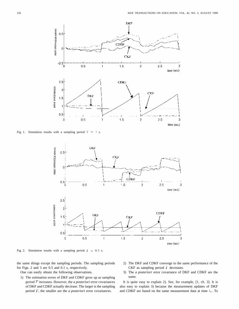
Fig. 2. Simulation results with a sampling periodT = 0:5 s.

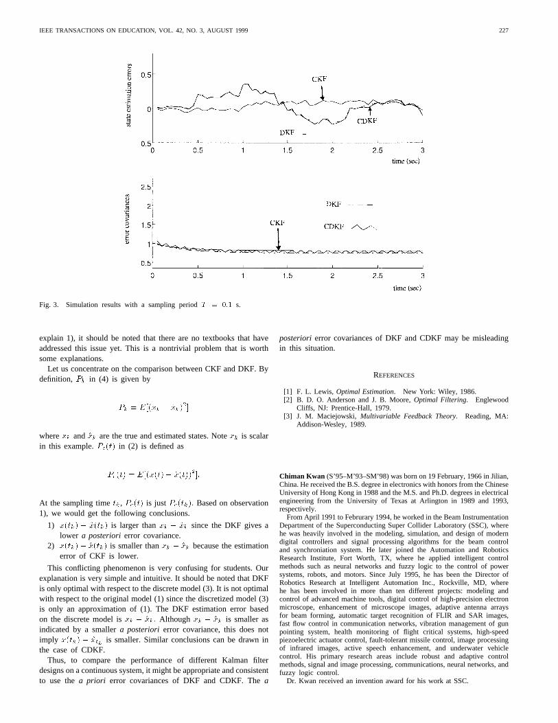
the same things except the sampling periods. The sampling periodsfor Figs. 2 and 3 are 0.5 and 0.1 s, respectively.

One can easily obtain the following observations.

1) The estimation errors of DKF and CDKF grow up as samplingperiodT increases. However, thea posteriorierror covariancesof DKF and CDKF actually decrease. The larger is the samplingperiodT , the smaller are thea posteriorierror covariances.

2) The DKF and CDKF converge to the same performance of theCKF as sampling periodT decreases.

3) The a posteriori error covariance of DKF and CDKF are thesame.

It is quite easy to explain 2). See, for example, [1, ch. 3]. It isalso easy to explain 3) because the measurement updates of DKFand CDKF are based on the same measurement data at timetk. To

IEEE TRANSACTIONS ON EDUCATION, VOL. 42, NO. 3, AUGUST 1999 227

Fig. 3. Simulation results with a sampling periodT = 0:1 s.

explain 1), it should be noted that there are no textbooks that haveaddressed this issue yet. This is a nontrivial problem that is worthsome explanations.

Let us concentrate on the comparison between CKF and DKF. Bydefinition, Pk in (4) is given by

Pk = E[(xk � xk)2]

wherexk and xk are the true and estimated states. Notexk is scalarin this example.Pc(t) in (2) is defined as

Pc(t) = E[(x(t)� x(t))2]:

At the sampling timetk, Pc(t) is justPc(tk): Based on observation1), we would get the following conclusions.

1) x(tk) � x(tk) is larger thanxk � xk since the DKF gives alower a posteriori error covariance.

2) x(tk)� x(tk) is smaller thanxk � xk because the estimationerror of CKF is lower.

This conflicting phenomenon is very confusing for students. Ourexplanation is very simple and intuitive. It should be noted that DKFis only optimal with respect to the discrete model (3). It is not optimalwith respect to the original model (1) since the discretized model (3)is only an approximation of (1). The DKF estimation error basedon the discrete model isxk � xk: Although xk � xk is smaller asindicated by a smallera posteriori error covariance, this does notimply x(tk) � xt is smaller. Similar conclusions can be drawn inthe case of CDKF.

Thus, to compare the performance of different Kalman filterdesigns on a continuous system, it might be appropriate and consistentto use thea priori error covariances of DKF and CDKF. Thea

posteriori error covariances of DKF and CDKF may be misleadingin this situation.

REFERENCES

[1] F. L. Lewis, Optimal Estimation. New York: Wiley, 1986.[2] B. D. O. Anderson and J. B. Moore,Optimal Filtering. Englewood

Cliffs, NJ: Prentice-Hall, 1979.[3] J. M. Maciejowski, Multivariable Feedback Theory. Reading, MA:

Addison-Wesley, 1989.

Chiman Kwan (S’95–M’93–SM’98) was born on 19 February, 1966 in Jilian,China. He received the B.S. degree in electronics with honors from the ChineseUniversity of Hong Kong in 1988 and the M.S. and Ph.D. degrees in electricalengineering from the University of Texas at Arlington in 1989 and 1993,respectively.

From April 1991 to Februrary 1994, he worked in the Beam InstrumentationDepartment of the Superconducting Super Collider Laboratory (SSC), wherehe was heavily involved in the modeling, simulation, and design of moderndigital controllers and signal processing algorithms for the beam controland synchroniation system. He later joined the Automation and RoboticsResearch Institute, Fort Worth, TX, where he applied intelligent controlmethods such as neural networks and fuzzy logic to the control of powersystems, robots, and motors. Since July 1995, he has been the Director ofRobotics Research at Intelligent Automation Inc., Rockville, MD, wherehe has been involved in more than ten different projects: modeling andcontrol of advanced machine tools, digital control of high-precision electronmicroscope, enhancement of microscope images, adaptive antenna arraysfor beam forming, automatic target recognition of FLIR and SAR images,fast flow control in communication networks, vibration management of gunpointing system, health monitoring of flight critical systems, high-speedpiezoelectric actuator control, fault-tolerant missile control, image processingof infrared images, active speech enhancement, and underwater vehiclecontrol. His primary research areas include robust and adaptive controlmethods, signal and image processing, communications, neural networks, andfuzzy logic control.

Dr. Kwan received an invention award for his work at SSC.

228 IEEE TRANSACTIONS ON EDUCATION, VOL. 42, NO. 3, AUGUST 1999

Frank L. Lewis (S’78–M’81–SM’86–F’94) was born in Wurzburg, Germany,subsequently studying in Chile and Scotland. He received the B.S. degree inphsics/electrical engineering and the Master’s of electrical engineering degreeat Rice University, Houston, TX, in 1971. In 1977, he received the Master’sof Science in aeronautical engineering from the University of West Florida,Pensacola. In 1981, he received the Ph.D. degree at the Georgia Institute ofTechnology, Atlanta.

He spent six years in the U.S. Navy, serving as a Navigator aboard thefrigate USS Trippe (FF-1075), and Executive Officer and Acting CommandingOfficer aboard USS Salinan (ATF-161). He was with the Georgia Instituteof Technology, Atlanta, from 1981 to 1990, and is currently an AdjunctProfessor. He was awarded the Moncrief-O’Donnel Endowed Chair in 1990at the Automation and Robotics Research Institute of The University ofTexas at Arlington. He has studied the geometric properties of the Riccatiequation and implicit systems. His current interests include robotics, intelligentcontrol, nonlinear systems, and manufacturing process control. He is theauthor/coauthor of more than 100 journal papers, more than 150 conferencepapers, and six books.

Dr. Lewis is a registered Professional Engineer in the State of Texas,Associate Editor ofCircuits, Systems, and Signal Processing, and the recipientof an NSF Research Initiation Grant, a Fulbright Research Award, theAmerican Society of Engineering Education F. E. Terman Award, three SigmaXi Research Awards, the UTA Halliburton Engineering Research Award, theUTA University-wide Distinguished Research Award, and the IEEE ControlSystems Society Best Chapter Award (as founding Chairman). He was selectedas Engineer of the Year in 1994 by the IEEE Fort Worth Section.

Concerning the Nyquist Plots ofRational Functions of Nonzero Type

Paulo J. S. G. Ferreira

Abstract—The Nyquist plots of rational functions of type one orhigher are often represented with branches that tend to infinity whileapproaching either the real or imaginary axis. It is shown that this failsto be true in general, a fact that appears to have little, if any, impact on theusual analysis. However, it has pedagogical interest since it explains thediscrepancy between the shape of the Nyquist plots obtained analytically,or with the help of computer programs in the classroom, and the plotsfound in many standard textbooks. The discrepancy is most clear whenthe system type is at least two, in which case the branches may moveinfinitely further from both axes.

Index Terms—Control engineering education, control systems, Nyquistplots.

I. INTRODUCTION

The Nyquist plot ofH(s) is the locus, in the complex plane, ofthe points1

fReH(j!); ImH(j!)g (1)

as a function of!. The traditional Nyquist plot of a rational functionH(s) of type one or higher often shows branches which tend toinfinity while approaching either the real or imaginary axis. Thisis, in general, incorrect. The purpose of this note is to discuss and

Manuscript received August 7, 1995; revised April 15, 1999.The author is with the Departamento de Electronica e Telecomunica¸coes,

Universidade de Aveiro, 3810 Aveiro, Portugal.Publisher Item Identifier S 0018-9359(99)06313-X.1The real and imaginary parts of a complexs are denoted byRes andIms,

respectively. The imaginary unit is denoted byj.

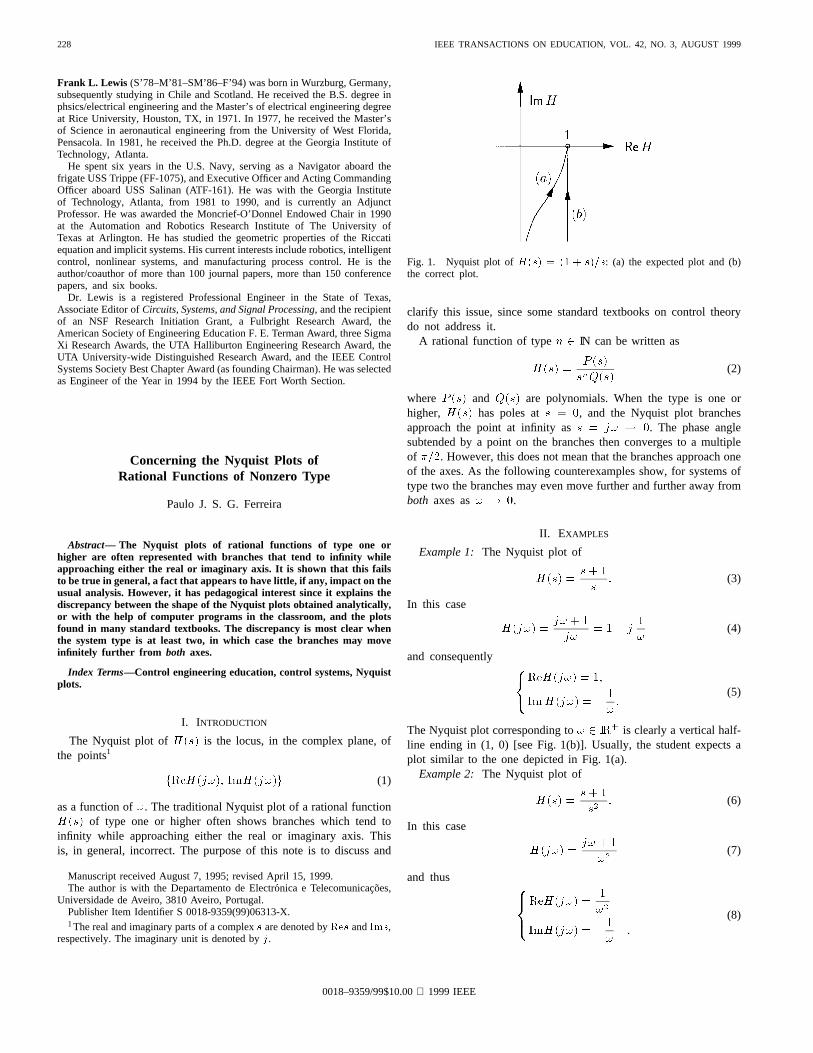
Fig. 1. Nyquist plot ofH(s) = (1 + s)=s: (a) the expected plot and (b)the correct plot.

clarify this issue, since some standard textbooks on control theorydo not address it.

A rational function of typen 2 IN can be written as

H(s) =P (s)

snQ(s)(2)

whereP (s) and Q(s) are polynomials. When the type is one orhigher, H(s) has poles ats = 0, and the Nyquist plot branchesapproach the point at infinity ass = j! ! 0. The phase anglesubtended by a point on the branches then converges to a multipleof �=2. However, this does not mean that the branches approach oneof the axes. As the following counterexamples show, for systems oftype two the branches may even move further and further away fromboth axes as! ! 0.

II. EXAMPLES

Example 1: The Nyquist plot of

H(s) =s+ 1

s: (3)

In this case

H(j!) =j! + 1

j!= 1� j

1

!(4)

and consequently

ReH(j!) = 1;

ImH(j!) = �1

!:

(5)

The Nyquist plot corresponding to! 2 IR+ is clearly a vertical half-line ending in (1, 0) [see Fig. 1(b)]. Usually, the student expects aplot similar to the one depicted in Fig. 1(a).

Example 2: The Nyquist plot of

H(s) =s+ 1

s2: (6)

In this case

H(j!) =j! + 1

�!2(7)

and thus

ReH(j!) =1

!2

ImH(j!) = �1

!.

(8)

0018–9359/99$10.00 1999 IEEE