A note on goodness-of-fit test of continuation ratio logistic regression models under case–control data

Journal of Statistical Planning and Inference 138 (2008) 2355–2365www.elsevier.com/locate/jspi

A note on goodness-of-fit test of continuation ratio logisticregression models under case–control data

Cheng Penga,∗, Biao Zhangb

aDepartment of Mathematics and Statistics, University of Southern Maine, Portland, ME 04104, USAbDepartment of Mathematics, The University of Toledo, Toledo, OH 43606, USA

Received 27 January 2006; received in revised form 18 June 2007; accepted 21 October 2007Available online 17 November 2007

Abstract

We extend the discussion of Qin and Zhang’s [1997. A goodness of fit test for logistic regression models base on case–control data.Biometrika 84, 609–618] goodness-of-fit test of logistic regression under case–control data to continuation ratio logistic regression(CRLR) models. We first showed that the retrospective CRLR model, which is valid for case–control data (the null hypothesis H0), isequivalent to an I-sample semiparametric model. Then under H0, we find the semiparametric profile empirical likelihood estimatorsof distributions of the covariate conditioning on each response category and use them to define a Kolmogorov–Smirnov type test forassessing the global fit of CRLR models under case–control data. Unlike prospective CRLR models, retrospective CRLR modelscannot be partitioned to a series of retrospective binary logistic regression models studied by Qin and Zhang [1997. A goodness offit test for logistic regression models base on case–control data. Biometrika 84, 609–618].© 2007 Elsevier B.V. All rights reserved.

Keywords: Continuation ratio logistics regression (CRLR); Case–control study; Asymptotic normality; Kolmogorov–Smirnov test; Bootstrap;Simulation

1. Introduction

In categorical regression we are interested in modelling the probability of the response taking a specific value,�i (x) = P(Y = i|X = x), where Y is the response variable, X is the vector of covariates and i is the ith category of theresponse, i = 1, 2, . . . , I . A continuation ratio logistic regression (CRLR) model, one of the parallel generalizations ofstandard binary logistic regression model, is defined in either one of the following forms:

logitP(Y = i|X = x)

P (Y � i|X = x)= �i + ��

i x for i = 1, . . . , I − 1 (1)

or

logitP(Y = i|X = x)

P (Y � i|X = x)= �i + ��

i x for i = 2, 3, . . . , I , (2)

where �i and ��i are parameters to be estimated. ��

i is a vector of parameters with the same dimension as that ofX. When I = 2, models (1) and (2) reduce to the standard binary logistic regression model. Since the cumulative

∗ Corresponding author. Tel.: +1 207 780 4689; fax: +1 207 780 5607.E-mail address: [email protected] (C. Peng).

0378-3758/$ - see front matter © 2007 Elsevier B.V. All rights reserved.doi:10.1016/j.jspi.2007.10.016

http://www.elsevier.com/locate/jspi

mailto:[email protected]

2356 C. Peng, B. Zhang / Journal of Statistical Planning and Inference 138 (2008) 2355–2365

probability P(Y � i|X = x) and P(Y � i|X = x) are used in definitions (1) and (2), CRLR models are useful to modelordinal response variables. Since CRLR models are “irreversible”, the two continuation ratio models (1) and (2) arenot equivalent (Hemker et al., 2001). The irreversibility of the response categories in CRLR models also implies thatthe CRLR models are especially useful when the response has a natural hierarchical structure.

Recently, the CRLR models have received considerable attention from researchers in different areas such as medicalresearch (Cox, 1988; Dos Santos and Berridge, 2000), ecological studies (Manel and Debouzie, 1997), fishery industry(Kvist et al., 2000), education and psychometrics (Hemker et al., 2001), etc. The existing procedures on these modelswere developed based on prospective sampling plans. In practice, there are situations in which data are collectedretrospectively. Any statistical procedure used on retrospective data needs to be adjusted accordingly. In this note, weonly work on continuation ratio model (1). The main focus of this note is to develop a goodness-of-fit test for assessingadequacy of CRLR models defined based on (1) under case–control sampling schemes. That is, we will test the nullhypothesis that the CRLR model is adequate for the case–control data.

The rest of the note is organized as follows. In Section 2, we develop the equivalence between the CRLR model undercase–control data and an I-sample semiparametric model and propose an empirical likelihood based semiparametricestimation procedure for model parameters. A goodness-of-fit test of the CRLR with case–control data is discussed inSection 3. In Section 4, we proposed a bootstrap procedure and present two examples. A simulation study is conductedin Section 5. Some concluding remarks are given in Section 6.

2. Model reparametrization and semiparametric MLE

Let {Xi1, Xi2, . . . , Xini} be the random sample collected from the ith population (ith category of Y) for i = 1, . . . , I .

Assume further that these samples are jointly independent. Denote P(Y = i) = �i , the population proportion of ithcategory, for i = 1, . . . , I . According to Bayes Theorem, we have

P(X|Y = i) = P(Y = i|X) · P(X)

P (Y = i)= �i (X)P (X)

P (Y = i). (3)

Re-expressing (2) in terms of �i (x) and solving for �i (x) by using the fact that∑I

i=1 �i (x) = 1, and plugging �i (x) in(3), we get

P(X|Y = i) = {exp(�i + ��i x) + I[i=I ]}

i∏l=1

1

1 + exp(�l + ��l x)

P (X)

�i

,

where I[i=I ] is an indicator function taking value 1 when i = I and 0 otherwise. Let fi(x) and f (x) be the densityfunctions of X given that Y = i and X, respectively. Then we have, for i = 1, . . . , I − 1,

fi(x) = �I

�i

exp(�i + ��i x)

1 + exp(�i + ��i x)

I−1∏l=i

[1 + exp(�l + ��l x)] · fI (x)

= exp[�i + gi(x, �)] · fI (x), (4)

where �i = (�i , ��i )

�, � = (��1, . . . , �

�I−1)

�, � = (�1, �2, . . . , �I−1)�, �i = log(�I /�i ), and

gi(x, �) ={�i + ��

i x +∑I−1l=i+1 log[1 + exp(�l + ��x)], i = 1, . . . , I − 2,

�I−1 + ��I−1x otherwise.

(5)

It is very different from the generalized logit model, another parallel generalization of the binary logistic regressionmodel, under retrospective data discussed in Zhang (2002) in which all intercept parameters, baseline logit �i , in thelinear predictor component and log ratio of subpopulation proportions, �i = log(�i/�I ), are inestimable. In retrospectiveCRLR models, all intercept parameters in the linear predictor component are estimable except the first intercept �1because �1 and �1 are linearly symmetric. Taking derivatives of the log-likelihood function with respect to �1 and �1yields the same score equation. With this in mind, we reexpress function gi(x, �) with form (7) and obtain the following

C. Peng, B. Zhang / Journal of Statistical Planning and Inference 138 (2008) 2355–2365 2357

identifiable I-sample semiparametric selection biased model which is equivalent to the CRLR model under case–controldata: ⎧⎨

⎩XI1, . . . , XInI

i.i.d.∼ fI (x),

Xi1, . . . , Xini

i.i.d.∼ exp(�i + gi(x, �)) · fI (x) for i = 1, . . . , I − 1,

(6)

where

gi(x, �) =

⎧⎪⎨⎪⎩

��1x +∑I−1

l=2 log[1 + exp(�l + ��x)], i = 1,

�i + ��i x +∑I−1

l=i+1 log[1 + exp(�l + ��x)], i = 2, . . . , I − 2,

�I−1 + ��I−1x otherwise.

(7)

The identifiability of the model follows from Theorem 2 of Gilbert et al. (1999) by checking the first weight functionin the I-sample selection biased semiparametric model (6).

When I = 2, model (6) degenerates to the retrospective binary logistic regression model studied by Qin and Zhang(1997). In the rest of the discussion, we assume the case that the response variable has more than two categories.

2.1. A semiparametric empirical maximum likelihood estimation procedure

For i =1, . . . , I , let Gi(x) be the corresponding cumulative distribution of fi(x), {T1, . . . , Tn} be the pooled sample{X11, . . . , X1n1; . . . ; XI1, . . . , XInI

} with n =∑Ii=1 ni , and Gi(t) be the empirical cumulative distribution function

(ECDF) defined based on the ith sample {Xi1, Xi2, . . . , Xini}. Then from model (6), we have following likelihood

function:

L(�, �, GI |X) =⎡⎣I−1∏

i=1

ni∏j=1

exp(�i + gi(Xij ; �)) dGI (Xij )

⎤⎦⎡⎣ nI∏

j=1

dGI (XIj )

⎤⎦

=n∏

s=1

ps

I−1∏i=1

ni∏j=1

{exp[�i + gi(Xij ; �)]}, (8)

where ps = dGI (ts) is the empirical likelihood of GI (X) at point ts with∑n

s=1 ps = 1, and gi(x; �) is specified in (7)for i = 1, 2, . . . , I . Its corresponding log-likelihood function is

l(�, �, GI ) =n∑

s=1

log ps +I−1∑i=1

ni�i +I−1∑i=1

ni∑j=1

gi(Xij , �). (9)

The estimates of parameters �, �i and the distribution GI (x) corresponding to the density function fI (x) will beobtained by maximizing l(�, �, GI ) subject to the following constraints, for s = 1, 2, . . . , n, i = 1, 2, . . . , I − 1,

1. ps �0, 2.

n∑s=1

ps = 1, 3.

n∑s=1

ps{exp[�i + gi(Ts; �)] − 1} = 0.

We first use Lagrange Multipliers to maximize the log-likelihood function (9) with given constraints by fixing parametersfirst and get profile MLE of ps

ps = 1

nI

· 1

1 +∑I−1i=1 �i exp[�i + gi(Ts; �)] , (10)

where �i = ni/nI for i = 1, 2, . . . , I − 1. One can see that ps is a function of data values and unknown parameters �and �. In (9) we substitute ps for ps and get the following semiparametric profile empirical log likelihood function

l(�, �) = −n log nI −n∑

s=1

log

{1 +

I−1∑i=1

�i exp[�i + gi(Ts; �)]}

+I−1∑i=1

ni∑j=1

[gi(Xij , �) + �i].


The corresponding score equations are given by, for u = 1, 2, 3, . . . , I − 1,

nu −n∑

s=1

�u exp[�u + gu(Ts; �)]1 +∑I−1

m=1 �m exp[�m + gm(Ts, �)] = 0, (11)

I∑i=1

ni∑j=1

[�gi(Xij ; �)

��−∑I−1

m=1 �m exp[�m + gm(Xij ; �)] · �gm(Xij ; �)/��

1 +∑I−1m=1 �m exp[�m + gm(Xij ; �)]

]= 0. (12)

The semiparametric MLE of (�, �), denoted by (�, �), is a solution to the above system of score equations (11) and(12). The semiparametric MLE of ps , denoted by ps , can be written as, for s = 1, 2, . . . , n,

ps = 1

nI

· 1

1 +∑I−1i=1 �i exp[�i + gi(Ts; �)] . (13)

Based on the estimate ps , the semiparametric empirical likelihood estimators of Gi(x) under model (6) (i.e., under H0)

are, for i = 1, . . . , I − 1,

GI (t) =n∑

s=1

psI[Ts � t], Gi(t) =n∑

s=1

ps exp[�i + gi(Ts; �)]I[Ts � t]. (14)

2.2. Asymptotic normality of estimators (�, �)

The consistency of the semiparametric profile empirical maximum likelihood estimators obtained based on H0, i.e.,model (6), can be proved by using the same arguments of Prentice and Pyke (1979). Before we present the asymptoticnormality of the proposed semiparametric estimator, we first define some notations.

We assume that ni/n approaches to a constant when n =∑Ii=1 ni → ∞, for i = 1, . . . , I . Denote �u = nu/nI , � =∑I

i=1 ni/nI , �I = 0, gI (x) = 0. Let (�0, �0) be the true value of (�, �). Furthermore, we define, for u, v = 1, 2, . . . , I ,

eu(x) = �u exp[�u + gu(x, �)]|�=�0,�=�0 , (15)

euv(x) = �u exp[�u + gu(x, �)]�v exp[�v + gv(x, �)]|�=�0,�=�0 , u �= v, (16)

euu(x) = −I∑

u�=v,v=1

euv(x) for u = 1, 2, . . . , I − 1, (17)

P(x) ={

1 +I−1∑m=1

�m exp[�m + gm(x, �)]}−1

∣∣∣∣∣∣�=�0,�=�0

, (18)

g��

u (x) = �gu(x, �)

��

∣∣∣∣�=�0

, g�u(x) = �gu(x, �)

��

∣∣∣∣�=�0

, (19)

auv = − 1

1 + �

∫P(x)euv(x) dGI (x) for u �= v, (20)

auu = −I∑

u�=v,v=1

auv for u = 1, 2, . . . , I − 1. (21)


Consequently,

auI = − 1

1 + �

∫P(x)eu(x) dGI (x) =

I−1∑v=1

auv for u = 1, 2, . . . , I − 1, (22)

S1 = (auv)u,v=1,2,...,I−1, S2 = ((a(�)1 )�, (a(�)

2 )�, . . . , (a(�)I−1)

�)�, (23)

where

a(�)u = 1

1 + �

∫eu(x)

(g��

u (x) − P(x)

I−1∑m=1

em(x)g��

m (x)

)dGI (x), (24)

S3 = 1

1 + �

∫ (I−1∑m=1

g�m(x)g��

m (x)em(x) − P(x)

I−1∑m=1

em(x)g�m(x)

I−1∑m=1

em(x)g��

m (x)

)dGI (x), (25)

D = diag

(1

�1, . . . ,

1

�I

), S = 1

1 + �

(S1 S2

S�2 S3

), =

(D + U O1

O1 O2

), (26)

where U is the (I − 1)× (I − 1) matrix with all elements being 1, O1 is an [(I − 1)(p + 1)− 1]× (I − 1) zero matrix,O2 is an [(I − 1)(p + 1) − 1] × [(I − 1)(p + 1) − 1] zero matrix, p is the number of parameters in the CRLR model.For any differentiable function f (x, y), denote

�f (x0, y0)

�x= �f (x, y)

�x

∣∣∣∣ x=x0y=y0

,�2f (x0, y0)

�x�y= �2f (x, y)

�x�y

∣∣∣∣ x=x0y=y0

. (27)

Let Hn be the Hessian matrix and Sn = Hn(x)/n. A direct calculation shows that Sn→P S as n → ∞. Furthermore,if the I-sample semiparametric model (6) holds, that is, the CRLR model (1) is valid for a case–control data, and S−1

exists, by

n−1/2(

�l(�0, �0)

�� ,�l(�0, �0)

��

)�P→ N(0, V ), (28)

and√

n(�� − ��0 �

� − ��0)

� d→ N(0, ), (29)

where V = S − (1 + �)(S�1, S

�2)

�(D + U)(S�1, S

�2) and = S−1 − (1 + �).

3. A Kolmogorov–Smirnov type goodness-of-fit test procedure

The semiparametric profile maximum likelihood estimators obtained in Section 2 rely on the null hypothesis (H0)

that the CRLR model is valid for the case–control data. In this section we propose a Kolmogorov–Smirnov typegoodness-of-fit test to assess the adequacy of CRLR models under case–control data.

In addition to the notations given in (15)–(19), we denote, for i, j = 1, 2, . . . , I and k = 0, 3,

d1i (t) = (ei2(t), . . . , ei(I−1)(t))�, d3i (t) =

I−1∑m=1

eim(t)(g�i (t) − g�

m(t)), (30)

Bij (t) =∫ t

−∞P(x)eij (x) dGI (x), Aki(t) = 1

ni

∫ t

−∞P(x)dki(x) dGI (x). (31)

Under the assumption that CRLR model (6) is valid and S−1 exists, then we have

√n(G1 − G1, . . . , GI − GI )

� d→ (W1, . . . , WI )�, (32)


in RI , where (W1, . . . , WI )� is a multivariate Gaussian process with continuous sample path satisfying, for all s, t ∈ R

and i = 1, 2, . . . , I ,

E{Wi(t)} = 0,

E{Wi(s)Wi(t)} = 1 + �

�2i

{�iGi(s ∧ t) − Bii(s ∧ t)} − 1

�2i

(A�1i (s), A

�2i (s))S

−1(

A1i (t)

A2i (t)

),

E{Wi(s)Wj (t)} = −1 + �

�i�j

Bij (s ∧ t) − 1

�i�j

(A�1i (s), A

�2i (s))S

−1(

A1j (t)

A2j (t)

),

where Gi(t) is the ECDF and Gi(t) is the semiparametric profile empirical maximum likelihood estimators of{Gi(t)}i=1,2,...,I under H0 with the explicit expression given in (14). The idea of derivation for the weak conver-gence results is similar to the proof of the weak convergence Theorem 3.2 in Zhang (2002). Details of deriving theasymptotic normality of (�, �) and the weak convergence

√n(G1 − G1, . . . , GI − GI )

� can be found in Peng (2003).A direct application of the above weak convergence of

√n(G1 − G1, . . . , GI − GI )

� for i = 1, 2, . . . , I , is to allowus using the discrepancy between Gi and Gi (for all i) to assess the adequacy of model (6). To be more specific, wedefine the distance between the pair of consistent estimators Gi(t) and Gi(t) to be the Euclidean super norm, and thediscrepancy of the two consistent estimators, Gi(t) and Gi(t), of Gi(x) is defined as �ni = sup−∞� t �∞ |√n(Gi(t)−Gi(t))|, i = 1, 2, . . . , I . We use the weighted average of the �ni as employed by Zhang (2002) and define the teststatistic as

�n = 1

I

I∑i=1

�i sup−∞� t �∞

|√n(Gi(t) − Gi(t))|. (33)

Since it is hard to find the sampling distribution with an explicit analytic expression of the above test statistic, themodified bootstrap re-sampling procedure (see Efron and Tibshirani, 1993) will be used to find the critical values inthe following section.

4. A bootstrap procedure and numerical examples

We will give very brief steps for taking bootstrap samples. We first generate bootstrap samples from G1, . . . , GI ,respectively, where Gi is the semiparametric empirical likelihood estimate of Gi . To be specific, let {X∗

i1, X∗i2, . . . , X

∗ini

}be an independent random sample generated from Gi for i = 1, 2, . . . , I . Assume further that {X∗

i1, X∗i2, . . . , X

∗ini

} fori = 1, 2, . . . , I , are jointly independent. Let {T ∗

1 , T ∗2 , . . . , T ∗

n } be the combined bootstrap sample {X∗11, . . . , X

∗1n1

; . . .

; X∗I1, X

∗I2, . . . , X

∗InI

}. We repeat the empirical likelihood based semiparametric profile likelihood estimation procedure

proposed in Section 2 to find bootstrap version estimates of parametric and non-parametric parts. Let (�∗, �∗)be solutionsto the bootstrap version of score equations and G∗

i (t) be the empirical cumulative distribution for the bootstrap sample{X∗

i1, X∗i2, . . . , X

∗ini

}, for i = 1, . . . , I . Furthermore, for s = 1, . . . , n, denote

p∗s = 1

nI

· 1

1 +∑I−1i=1 �i exp[�∗

i + gi(T ∗s ; �

∗)]

, (34)

and for i = 1, . . . , I − 1,

G∗I (t) =

n∑s=1

p∗s I[T ∗

s � t], G∗i (t) =

n∑s=1

p∗s exp[�∗

i + gi(T∗s ; �

∗)]I[T ∗

s � t]. (35)

The Kolmogorov–Smirnov test statistic based on the bth bootstrap sample is �∗bn = (1/I)

∑Ii=1 �isup−∞� t �∞ |√

n(G∗bi (t) − G∗b

i (t))|. The bootstrap p-value of the proposed Kolmogorov–Smirnov test is defined by pboot =#{�∗b

n ��n}/B, where �n is the value calculated from the sample data set and B the number of bootstrap samples.


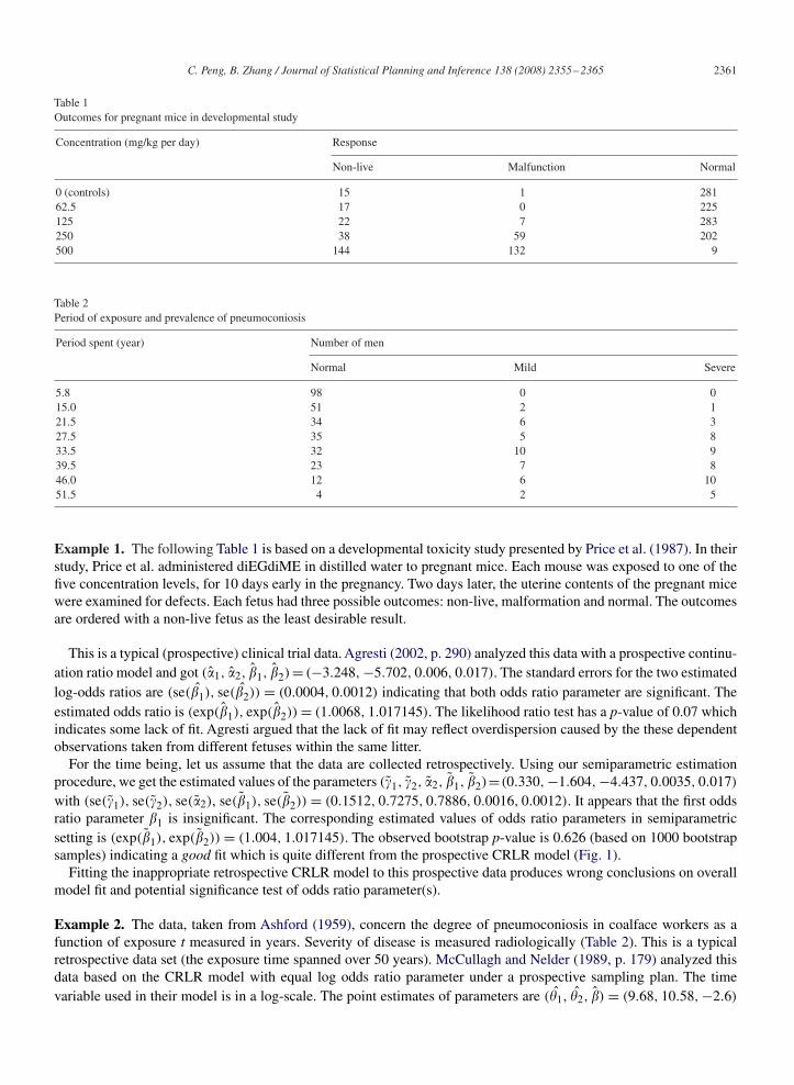
Table 1Outcomes for pregnant mice in developmental study

Concentration (mg/kg per day) Response

Non-live Malfunction Normal

0 (controls) 15 1 28162.5 17 0 225125 22 7 283250 38 59 202500 144 132 9

Table 2Period of exposure and prevalence of pneumoconiosis

Period spent (year) Number of men

Normal Mild Severe

5.8 98 0 015.0 51 2 121.5 34 6 327.5 35 5 833.5 32 10 939.5 23 7 846.0 12 6 1051.5 4 2 5

Example 1. The following Table 1 is based on a developmental toxicity study presented by Price et al. (1987). In theirstudy, Price et al. administered diEGdiME in distilled water to pregnant mice. Each mouse was exposed to one of thefive concentration levels, for 10 days early in the pregnancy. Two days later, the uterine contents of the pregnant micewere examined for defects. Each fetus had three possible outcomes: non-live, malformation and normal. The outcomesare ordered with a non-live fetus as the least desirable result.

This is a typical (prospective) clinical trial data. Agresti (2002, p. 290) analyzed this data with a prospective continu-ation ratio model and got (�1, �2, �1, �2)= (−3.248, −5.702, 0.006, 0.017). The standard errors for the two estimatedlog-odds ratios are (se(�1), se(�2)) = (0.0004, 0.0012) indicating that both odds ratio parameter are significant. Theestimated odds ratio is (exp(�1), exp(�2)) = (1.0068, 1.017145). The likelihood ratio test has a p-value of 0.07 whichindicates some lack of fit. Agresti argued that the lack of fit may reflect overdispersion caused by the these dependentobservations taken from different fetuses within the same litter.

For the time being, let us assume that the data are collected retrospectively. Using our semiparametric estimationprocedure, we get the estimated values of the parameters (�1, �2, �2, �1, �2)=(0.330, −1.604, −4.437, 0.0035, 0.017)

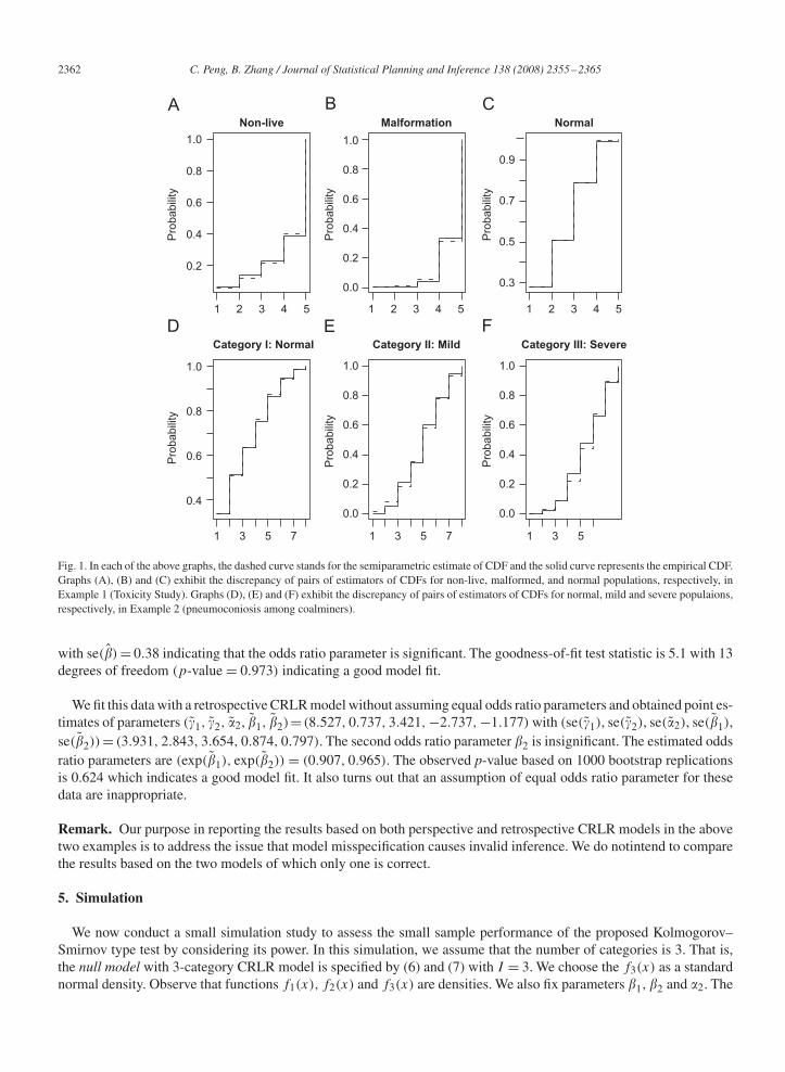
with (se(�1), se(�2), se(�2), se(�1), se(�2)) = (0.1512, 0.7275, 0.7886, 0.0016, 0.0012). It appears that the first oddsratio parameter �1 is insignificant. The corresponding estimated values of odds ratio parameters in semiparametricsetting is (exp(�1), exp(�2)) = (1.004, 1.017145). The observed bootstrap p-value is 0.626 (based on 1000 bootstrapsamples) indicating a good fit which is quite different from the prospective CRLR model (Fig. 1).

Fitting the inappropriate retrospective CRLR model to this prospective data produces wrong conclusions on overallmodel fit and potential significance test of odds ratio parameter(s).

Example 2. The data, taken from Ashford (1959), concern the degree of pneumoconiosis in coalface workers as afunction of exposure t measured in years. Severity of disease is measured radiologically (Table 2). This is a typicalretrospective data set (the exposure time spanned over 50 years). McCullagh and Nelder (1989, p. 179) analyzed thisdata based on the CRLR model with equal log odds ratio parameter under a prospective sampling plan. The timevariable used in their model is in a log-scale. The point estimates of parameters are (�1, �2, �) = (9.68, 10.58, −2.6)


1

0.2

0.4

0.6

0.8

1.0

Non-live

Probability

0.0

0.2

0.4

0.6

0.8

1.0

Malformation

Probability

0.3

0.5

0.7

0.9

Normal

Probability

1 7

0.4

0.6

0.8

1.0

Category I: Normal

Probability

0.0

0.2

0.4

0.6

0.8

1.0

Category II: Mild

Probability

0.0

0.2

0.4

0.6

0.8

1.0

Category III: Severe

Probability

2 3 4 5 1 2 3 4 5 1 2 3 4 5

3 5 1 73 5 1 3 5

Fig. 1. In each of the above graphs, the dashed curve stands for the semiparametric estimate of CDF and the solid curve represents the empirical CDF.Graphs (A), (B) and (C) exhibit the discrepancy of pairs of estimators of CDFs for non-live, malformed, and normal populations, respectively, inExample 1 (Toxicity Study). Graphs (D), (E) and (F) exhibit the discrepancy of pairs of estimators of CDFs for normal, mild and severe populaions,respectively, in Example 2 (pneumoconiosis among coalminers).

with se(�) = 0.38 indicating that the odds ratio parameter is significant. The goodness-of-fit test statistic is 5.1 with 13degrees of freedom (p-value = 0.973) indicating a good model fit.

We fit this data with a retrospective CRLR model without assuming equal odds ratio parameters and obtained point es-timates of parameters (�1, �2, �2, �1, �2)= (8.527, 0.737, 3.421, −2.737, −1.177) with (se(�1), se(�2), se(�2), se(�1),se(�2))= (3.931, 2.843, 3.654, 0.874, 0.797). The second odds ratio parameter �2 is insignificant. The estimated oddsratio parameters are (exp(�1), exp(�2)) = (0.907, 0.965). The observed p-value based on 1000 bootstrap replicationsis 0.624 which indicates a good model fit. It also turns out that an assumption of equal odds ratio parameter for thesedata are inappropriate.

Remark. Our purpose in reporting the results based on both perspective and retrospective CRLR models in the abovetwo examples is to address the issue that model misspecification causes invalid inference. We do notintend to comparethe results based on the two models of which only one is correct.

5. Simulation

We now conduct a small simulation study to assess the small sample performance of the proposed Kolmogorov–Smirnov type test by considering its power. In this simulation, we assume that the number of categories is 3. That is,the null model with 3-category CRLR model is specified by (6) and (7) with I = 3. We choose the f3(x) as a standardnormal density. Observe that functions f1(x), f2(x) and f3(x) are densities. We also fix parameters �1, �2 and �2. The


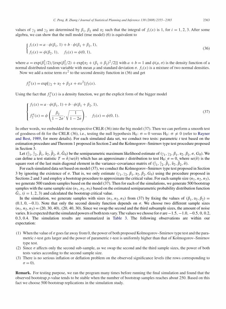
values of �2 and �2 are determined by �1, �2 and �2 such that the integral of fi(x) is 1, for i = 1, 2, 3. After somealgebra, we can show that the null model (true model) (6) is equivalent to

{f1(x) = a · �(�1, 1) + b · �(�1 + �2, 1),

f2(x) = �(�2, 1), f3(x) = �(0, 1),(36)

where a = exp(�21/2)/{exp(�2

1/2) + exp[�2 + (�1 + �2)2/2]} with a + b = 1 and �( , �) is the density function of a

normal distributed random variable with mean and standard deviation �. f1(x) is a mixture of two normal densities.Now we add a noise term �x2 to the second density function in (36) and get

f �2 (x) = exp[�2 + �2 + �2x + �x2]f3(x).

Using the fact that f �2 (x) is a density function, we get the explicit form of the bigger model

⎧⎪⎨⎪⎩

f1(x) = a · �(�1, 1) + b · �(�1 + �2, 1),

f �2 (x) = �

(�2

1 − 2�,

√1

1 − 2�

), f3(x) = �(0, 1).

(37)

In other words, we embedded the retrospective CRLR (36) into the big model (37). Then we can perform a smooth testof goodness-of-fit for the CRLR (36), i.e., testing the null hypothesis H0 : � = 0 versus H0 : � �= 0 (refer to Raynerand Best, 1989, for more details). For each simulated data set, we conduct two tests: parametric t test based on theestimation procedure and Theorem 1 proposed in Section 2 and the Kolmogorov–Smirnov type test procedure proposedin Section 3.

Let (�1, �2, �1, �2, �2, �, G0) be the semiparametric maximum likelihood estimate of (�1, �2, �1, �2, �2, �, G0). Wecan define a test statistic T = �/se(�) which has an approximate t distribution to test H0: � = 0, where se(�) is thesquare root of the last main diagonal element in the variance–covariance matrix of (�1, �2, �1, �2, �2, �).

For each simulated data set based on model (37), we conduct the Kolmogorov–Smirnov type test proposed in Section3 by ignoring the existence of �. That is, we only estimate (�1, �2, �1, �2, �2, G0) using the procedure proposed inSections 2 and 3 and employ a bootstrap procedure to approximate the critical value. For each sample size (n1, n2, n3),we generate 500 random samples based on the model (37). Then for each of the simulations, we generate 500 bootstrapsamples with the same sample size (n1, n2, n3) based on the estimated semiparametric probability distribution functionGi, (i = 1, 2, 3) and calculated the bootstrap critical value.

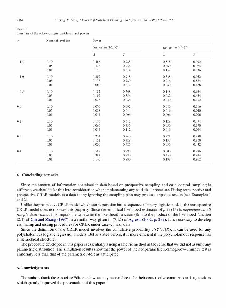
In the simulation, we generate samples with sizes (n1, n2, n3) from (37) by fixing the values of (�1, �2, �2) =(0.1, 0, −0.1). Note that only the second density function depends on �. We choose two different sample sizes(n1, n2, n3) = (20, 30, 40), (20, 40, 30). Since we swap the second and the third subsample sizes, the amount of noisevaries. It is expected that the simulated powers of both tests vary.The values we choose for� are−1.5, −1.0, −0.5, 0, 0.2,

0.3, 0.4. The simulation results are summarized in Table 3. The following observations are within ourexpectation:

(1) When the value of � goes far away from 0, the power of both proposed Kolmogorov–Smirnov type test and the para-metric t-test gets larger and the power of parametric t-test is uniformly higher than that of Kolmogorov–Smirnovtype test.

(2) Since � affects only the second sub-sample, as we swap the second and the third sample sizes, the power of bothtests varies according to the second sample size.

(3) There is no serious inflation or deflation problem on the observed significance levels (the rows corresponding to� = 0).

Remark. For testing purpose, we ran the program many times before running the final simulation and found that theobserved bootstrap p-value tends to be stable when the number of bootstrap samples reaches about 250. Based on thisfact we choose 500 bootstrap replications in the simulation study.


Table 3Summary of the achieved significant levels and powers

� Nominal level (�) Power

(n2, n3) = (30, 40) (n2, n3) = (40, 30)

� T � T

−1.5 0.10 0.486 0.988 0.518 0.9920.05 0.328 0.956 0.360 0.9740.01 0.138 0.514 0.152 0.736

−1.0 0.10 0.302 0.918 0.328 0.9520.05 0.178 0.780 0.216 0.8640.01 0.060 0.272 0.080 0.476

−0.5 0.10 0.182 0.568 0.148 0.6340.05 0.102 0.356 0.082 0.4540.01 0.028 0.086 0.020 0.102

0.0 0.10 0.070 0.092 0.086 0.1160.05 0.038 0.044 0.046 0.0400.01 0.014 0.006 0.006 0.006

0.2 0.10 0.116 0.512 0.128 0.4940.05 0.066 0.336 0.056 0.3700.01 0.014 0.112 0.016 0.084

0.3 0.10 0.234 0.840 0.221 0.8880.05 0.122 0.728 0.133 0.8000.01 0.030 0.426 0.036 0.432

0.4 0.10 0.508 0.990 0.600 0.9960.05 0.362 0.980 0.450 0.9940.01 0.140 0.890 0.198 0.912

6. Concluding remarks

Since the amount of information contained in data based on prospective sampling and case–control sampling isdifferent, we should take this into consideration when implementing any statistical procedure. Fitting retrospective andprospective CRLR models to a data set by ignoring the sampling plan may produce opposite results (see Examples 1and 2).

Unlike the prospective CRLR model which can be partition into a sequence of binary logistic models, the retrospectiveCRLR model does not posses this property. Since the empirical likelihood estimator of p in (13) is dependent on allsample data values, it is impossible to rewrite the likelihood function (8) into the product of the likelihood function(2.1) of Qin and Zhang (1997) in a similar way given in (7.15) of Agresti (2002, p. 289). It is necessary to developestimating and testing procedures for CRLR under case–control data.

Since the definition of the CRLR model involves the cumulative probability P(Y � i|X), it can be used for anypolychotomous logistic regression models. But as stated before, it is more efficient if the polychotomous response hasa hierarchical structure.

The procedure developed in this paper is essentially a nonparametric method in the sense that we did not assume anyparametric distribution. The simulation results show that the power of the nonparametric Kolmogorov–Smirnov test isuniformly less than that of the parametric t-test as anticipated.

Acknowledgments

The authors thank the Associate Editor and two anonymous referees for their constructive comments and suggestionswhich greatly improved the presentation of this paper.


References

Agresti, A., 2002. Categorical Data Analysis. Wiley, New York.Ashford, J.R., 1959. An approach to the analysis of data for semiquantal responses in biological assay. Biometrics 15, 573–581.Cox, C., 1988. Multinomial regression models based on continuation ratios. Statist. Med. 7, 435–442.Dos Santos, D., Berridge, D., 2000. A continuation ratio random effects model for repeated ordinal responses. Statist. Med. 19, 3377–3388.Efron, B., Tibshirani, R., 1993. An Introduction to the Bootstrap. Chapman & Hall, London.Gilbert, P., Lele, S., Vardi,Y., 1999. Maximum likelihood estimation in semiparametric selecion bias models with application to AIDS vaccine trials.

Biometrika 86, 27–43.Hemker, B., van der Ark, L., Sijtsma, K., 2001. On measurement properties of continuation ratio models. Psychometrika 66 (4), 487–506.Kvist, T., Gilason, H., Thyregod, P., 2000. Using continuation ratio logits to analyse the variation of the age-composition of fish catches. J. Appl.

Statist. 27, 303–319.Manel, S., Debouzie, D., 1997. Logistic regression and continuation ratio models to estimate insect development under variable tempratures. Ecol.

Modelling 98, 237–243.McCullagh, P., Nelder, J.A., 1989. Generalized Linear Models. Chapman & Hall, London.Peng, C., 2003. Fitting and testing continuation ratio logistic regression models under case–control data. Ph.D. Dissertation. The University of

Toledo.Prentice, R.L., Pyke, R., 1979. Logistic disease incidence models and case–control studies. Biometrika 66, 403–411.Price, C.J., Kimmel, C.A., George, J.D., Marr, M.C., 1987. The developmental toxicity of diethylene glycol dimethyl ether in mice. Fund. Appl.

Toxicol. 8, 115–126.Qin, J., Zhang, B., 1997. A goodness of fit test for logistic regression models base on case–control data. Biometrika 84, 609–618.Rayner, J.C.W., Best, D.J., 1989. Smooth Tests of Goodness of Fit. Oxford University Press, Oxford.Zhang, B., 2002. Assessing the goodness-of-fit of the generalized logit models based on case control data. J. Multivariate Anal. 82, 17–38.

Documents

A note on goodness-of-fit test of continuation ratio logistic regression models under case–control data