A normalization strategy for comparing tag count data

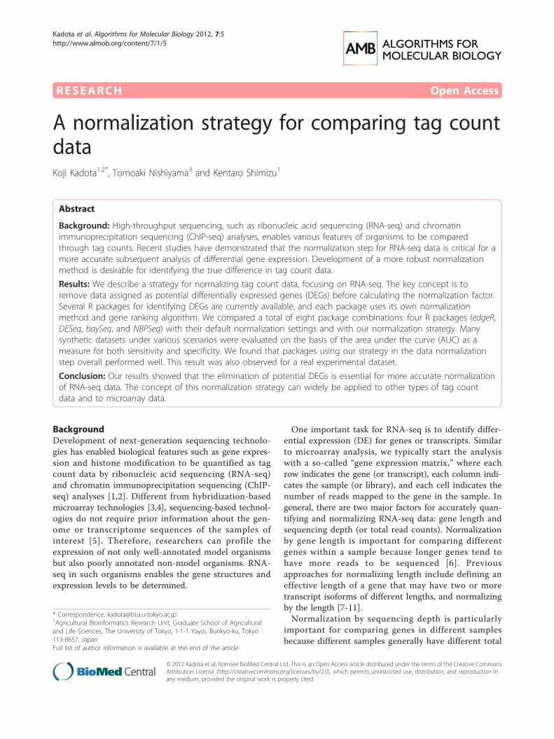
RESEARCH Open Access

A normalization strategy for comparing tag countdataKoji Kadota1,2*, Tomoaki Nishiyama3 and Kentaro Shimizu1

Abstract

Background: High-throughput sequencing, such as ribonucleic acid sequencing (RNA-seq) and chromatinimmunoprecipitation sequencing (ChIP-seq) analyses, enables various features of organisms to be comparedthrough tag counts. Recent studies have demonstrated that the normalization step for RNA-seq data is critical for amore accurate subsequent analysis of differential gene expression. Development of a more robust normalizationmethod is desirable for identifying the true difference in tag count data.

Results: We describe a strategy for normalizing tag count data, focusing on RNA-seq. The key concept is toremove data assigned as potential differentially expressed genes (DEGs) before calculating the normalization factor.Several R packages for identifying DEGs are currently available, and each package uses its own normalizationmethod and gene ranking algorithm. We compared a total of eight package combinations: four R packages (edgeR,DESeq, baySeq, and NBPSeq) with their default normalization settings and with our normalization strategy. Manysynthetic datasets under various scenarios were evaluated on the basis of the area under the curve (AUC) as ameasure for both sensitivity and specificity. We found that packages using our strategy in the data normalizationstep overall performed well. This result was also observed for a real experimental dataset.

Conclusion: Our results showed that the elimination of potential DEGs is essential for more accurate normalizationof RNA-seq data. The concept of this normalization strategy can widely be applied to other types of tag countdata and to microarray data.

BackgroundDevelopment of next-generation sequencing technolo-gies has enabled biological features such as gene expres-sion and histone modification to be quantified as tagcount data by ribonucleic acid sequencing (RNA-seq)and chromatin immunoprecipitation sequencing (ChIP-seq) analyses [1,2]. Different from hybridization-basedmicroarray technologies [3,4], sequencing-based technol-ogies do not require prior information about the gen-ome or transcriptome sequences of the samples ofinterest [5]. Therefore, researchers can profile theexpression of not only well-annotated model organismsbut also poorly annotated non-model organisms. RNA-seq in such organisms enables the gene structures andexpression levels to be determined.

One important task for RNA-seq is to identify differ-ential expression (DE) for genes or transcripts. Similarto microarray analysis, we typically start the analysiswith a so-called “gene expression matrix,” where eachrow indicates the gene (or transcript), each column indi-cates the sample (or library), and each cell indicates thenumber of reads mapped to the gene in the sample. Ingeneral, there are two major factors for accurately quan-tifying and normalizing RNA-seq data: gene length andsequencing depth (or total read counts). Normalizationby gene length is important for comparing differentgenes within a sample because longer genes tend tohave more reads to be sequenced [6]. Previousapproaches for normalizing length include defining aneffective length of a gene that may have two or moretranscript isoforms of different lengths, and normalizingby the length [7-11].Normalization by sequencing depth is particularly

important for comparing genes in different samplesbecause different samples generally have different total

* Correspondence: [email protected] Bioinformatics Research Unit, Graduate School of Agriculturaland Life Sciences, The University of Tokyo, 1-1-1 Yayoi, Bunkyo-ku, Tokyo113-8657, JapanFull list of author information is available at the end of the article

Kadota et al. Algorithms for Molecular Biology 2012, 7:5http://www.almob.org/content/7/1/5

© 2012 Kadota et al; licensee BioMed Central Ltd. This is an Open Access article distributed under the terms of the Creative CommonsAttribution License (http://creativecommons.org/licenses/by/2.0), which permits unrestricted use, distribution, and reproduction inany medium, provided the original work is properly cited.

mailto:[email protected]

http://creativecommons.org/licenses/by/2.0

read counts. Previous approaches include (i) global scal-ing so that a summary statistic such as the mean orupper-quartile value of read counts for each sample (orlibrary) becomes a common value and (ii) standardiza-tion of distribution so that the read count distributionsbecome the same across samples [12-15]. Some groupsrecently reported that over-representation of genes withhigher expression in one of the samples, i.e., biased dif-ferential expression, has a negative impact on data nor-malization and consequently can lead to biasedestimates of true differentially expressed genes (DEGs)[15,16]. To reduce the effect of such genes on the datanormalization step, Robinson and Oshlack reported asimple but effective global scaling method, the trimmedmean of M values (TMM) method, where a scaling fac-tor for the normalization is calculated as a weightedtrimmed mean of the log ratios between two classes ofsamples (i.e., Samples A vs. B) [16]. The concept of theTMM method is the basis for developing our normaliza-tion strategy.In this paper, we focus on normalization related to

sequencing depth as well as the TMM normalizationmethod. We believe the TMM method can be improved.Consider, for example, a hypothetical dataset containinga total of 1000 genes, where (i) 200 genes (i.e., 200/1000= 20%) are detected as DEGs when comparing SamplesA vs. B (PDEG = 20%), (ii) 180 of the 200 DEGs arehighly expressed in Sample A (i.e., PA = 180/200 =90%), (iii) the dataset can be perfectly normalized byapplying a normalization factor calculated based only onthe remaining 800 non-DEGs, and (iv) individual DEGs(or non-DEGs) have a negative (or positive) impact oncalculation of the normalization factor. In this case, thetwo parameters should ideally be estimated as PDEG =20% and PA = 90%. Currently, the TMM method impli-citly uses fixed values for these two parameters (i.e.,PDEG = 60 and PA = 50) unless users explicitly providearbitrary values [16,17]. This is probably because anautomatic estimation of the PDEG value is practicallydifficult.Hardcastle and Kelly [18] recently proposed an R [19]

package, baySeq, for differential expression analysis ofRNA-seq data. A notable advantage of this method isthat an objective PDEG value is produced by calculatingmultiple models of differential expression. This methodalso inspired us in our improvement of the normaliza-tion of RNA-seq data. Our normalization strategy,named TbT, consists of TMM [16] and baySeq [18],used twice and once respectively in a TMM-baySeq-TMM pipeline. We show the importance of estimatingthe PDEG value according to the true PDEG value forindividual datasets. The results were obtained usingsimulated and real datasets.

Results and DiscussionRNA-seq data must be normalized before differentialexpression analysis can be conducted on them. Some Rpackages exist for comparing two groups of samples[17,18,20,21], and each package uses its own normaliza-tion method and gene ranking algorithm. For example,the R package edgeR [17] uses the TMM method [16]for data normalization and an exact test for negativebinomial (NB) distribution [22] for gene ranking. Agood normalization method coupled with gene rankingmethods should produce good ranked gene lists wheretrue DEGs can easily be detected as top-ranked andnon-DEGs are bottom-ranked, when all genes areranked according to the degree of DE.Following from our previous study [23-25], the area

under the receiver operating characteristic (ROC) curve(i.e., AUC) values were used for evaluating individualcombinations based on sensitivity and specificity simul-taneously. A good combination should therefore have ahigh AUC value (i.e., high sensitivity and specificity). Inthe remainder of this paper, we first describe our nor-malization strategy (called TbT). We then evaluate atotal of eight package combinations: four R packages fordifferential expression analysis (edgeR [17], DESeq [20],baySeq [18], and NBPSeq [21]) with default normaliza-tion settings (which we call edgeR/default, DESeq/default, baySeq/default, and NBPSeq/default) and thesame four packages with TbT normalization (i.e., edgeRcoupled with TbT (edgeR/TbT), DESeq/TbT, baySeq/TbT, and NBPSeq/TbT). Finally, we discuss guidelinesfor meaningful differential expression analysis.Note that the execution of the baySeq package was

performed using data after scaling for the reads per mil-lion (RPM) mapped reads in each sample. The proce-dure in the baySeq package and in the other threepackages (edgeR, DESeq, and NBPSeq) is not intendedfor use with RPM-normalized data, i.e., the original rawcount data should be used as the input. However, wefound that the use of RPM-normalized data generallyyields higher AUC values compared to the use of rawcount data when executing the baySeq package. We alsofound that the use of RPM data did not positively affectthe results when the other three packages were exe-cuted. Accordingly, all of the results relating to the bay-Seq package were obtained using the RPM-normalizeddata. This includes step 2 in the TbT normalization andthe gene ranking of DEGs using two baySeq-relatedcombinations (baySeq/TbT and baySeq/default).

Outline of TbT normalization strategyThe key feature of TbT is that data assigned as potentialDEGs are removed before the normalization factor iscalculated. We will explain the concept of TbT by using


Page 2 of 13

simulation data that are negative binomially distributed(three libraries from Sample A vs. three libraries fromSample B; i.e., {A1, A2, A3} vs. {B1, B2, B3}). The simula-tion conditions were that (i) 20% of genes were DEGs(PDEG = 20%), (ii) 90% of PDEG was higher in Sample A(PA = 90%), and (iii) the level of DE was four-fold.The NB model is generally applicable when the tag

count data are based on biological replicates. It has beennoted that the variance of biological replicate readcounts for a gene (V) is higher than the mean (μ) of theread counts (e.g., V = μ + jμ2 where j > 0) and thatthe extra dispersion parameter j tends to have large (orsmall) values when μ is small (or large) [20,21]. Tomimic this mean-dispersion relationship in the simula-tion, we used an empirical distribution of these values(μ and j) calculated from Arabidopsis data available inthe NBPSeq package [21]. For details, see the Methodssection.An M-A plot of the simulation data, after scaling for

RPM reads in each library, is shown in Figure 1a. Thehorizontal axis indicates the average expression level ofa gene across two groups, and the vertical axis indicateslog-ratios (Sample B relative to Sample A). As shown bythe black horizontal line, the median log-ratio for non-DEGs based on the RPM-normalized data (0.543) has aclear offset from zero due to the introduced DEGs with

the above three conditions. Therefore, the primary aimof our method is to accurately estimate the percentageof true DEGs (PDEG) and trim the corresponding DEGsso that the median log-ratio for non-DEGs is as close tozero as possible when our TbT normalization factorsare used.To accomplish this, our normalization method con-

sists of three steps: (1) temporary normalization, (2)identification of DEGs, and (3) final normalization ofdata after eliminating those DEGs. We used the TMMmethod [16] at steps 1 and 3 and an empirical Bayesianmethod implemented in the baySeq package [18] at step2. Other methods could have been used, but our choicesseemed to produce good ranked gene lists with highsensitivity and specificity (i.e., a high AUC value). Weobserved that the median log-ratio for non-DEGs basedon our TbT normalization factors (0.045) was closer tozero than the log-ratio based on the TMM normaliza-tion factors (0.170) that corresponds to the result ofTbT right after step 1 (Figure 1b).This result suggests the validity of our strategy of

removing potential DEGs before calculating the normali-zation factor. Recall that the true values for PDEG andPA in this simulation were 20% and 90%, respectively.Our TbT method estimated 16.8% of PDEG and 76.3% ofPA. We found that 64.4% of the estimated DEGs were

(a) (b)

Figure 1 Outline of TbT normalization strategy. Left panel: M-A plot for negative binomially distributed simulation data from Ref. [21], afterscaling for RPM mapped reads in each sample. Magenta and black dots indicate DEGs (20% of all genes; PDEG = 20%) and non-DEGs (80%),respectively. 90% of all DEGs is four-fold higher in Sample A than B (PA = 90%). Each dot represents a gene. Right panel: same plot but coloreddifferently. TbT estimates 16.8% of PDEG using this data. Gray dots indicate genes estimated as non-DEGs by step 2 in TbT. Note that the medianlog-ratio for true non-DEGs when data normalization is performed using the TbT normalization factors (0.045) is closer to zero than that usingthe TMM normalization factors (0.170).


Page 3 of 13

true DEGs (i.e., sensitivity = 64.4%) and that the overallaccuracy was 89.0%. Some researchers might think thatthe TMM method (i.e., PDEG = 60% and PA = 50%)must be able to remove many more true DEGs than ourTbT method (i.e., higher sensitivity). This is true, butthe TMM method tends to trim many more non-DEGsthan our method (i.e., lower specificity), especially whenmost DEGs are highly expressed in one of the samples(corresponding to our simulation conditions with highPDEG and PA values). These characteristics for the twonormalization methods and the results shown in Figure1 indicate that the balance of sensitivity and specificityregarding the assignment of both DEGs and non-DEGsis critical. Our TbT method was originally designed tonormalize tag count data for various scenarios includingsuch biased differential expression.The successful removal of DEGs in the data normali-

zation step generally increases both the sensitivity andspecificity of the subsequent differential expression ana-lysis. Indeed, when an exact test implemented in the Rpackage edgeR [17] was used in common for gene rank-ing, the TbT normalization method showed a higherAUC value (i.e., edgeR/TbT = 90.0%) than the default(the TMM method [16] in this package) normalizationmethod (i.e., edgeR/default = 88.9%). We also observedthe same trend for the other combinations: DESeq/TbT= 88.7%, DESeq/default = 87.4%, baySeq/TbT = 90.2%,baySeq/default = 78.2%, NBPSeq/TbT = 90.1%, andNBPSeq/default = 80.9%. These results also suggest thatour TbT normalization strategy can successfully becombined with the four existing R packages and thatthe TbT method outperforms the other normalizationmethods implemented in these packages.

Simulation resultsNote that different trials of simulation analysis generallyyield different AUC values even if the same simulationconditions are introduced. It is important to show thestatistical significance, if any, of our proposed method.The distributions of AUC values for two edgeR-relatedcombinations (edgeR/TbT and edgeR/default) underthree conditions (PA = 50, 70, and 90% with a fixedPDEG value of 20%) are shown in Figure 2. The perfor-mances between the two combinations were very similarwhen PA = 50% (Figure 2a; p-value = 0.95, Wilcoxonrank sum test). This is reasonable because the averageestimate of the PA values by TbT in the 100 trials(49.62%) was quite close to the truth (i.e., 50%) andTMM uses a fixed PA value of 50%. The higher the PAvalue (> 50%) TbT estimates, the higher the perfor-mance of TbT (compared to TMM) that can beexpected.Different from the above unbiased case (PA = 50%),

we observed the obvious superiority of TbT under the

other two conditions (PA = 70 and 90%). A significantimprovement resulting from use of TbT may seemdoubtful because of the very small difference betweenthe two average AUC values (e.g., 90.52% for edgeR/TbTand 90.26% for edgeR/default when PA = 70%; left panelof Figure 2b), but the edgeR/TbT combination did out-perform the edgeR/default combination in all of the 100trials under the two conditions (right panels of Figures2b and 2c), and the p-values were lower than 0.01 (Wil-coxon rank sum test).Table 1 shows the average AUC values for the two

edgeR-related combinations under the various simula-tion conditions (PDEG = 5-30% and PA = 50-100%).Overall, edgeR/TbT performed better than edgeR/defaultfor most of the simulation conditions analyzed. Therelative performance of TbT compared to the defaultmethod (i.e., the TMM method [16] in this case) can beseen to improve according to the increased PA valuesstarting from 50%. This is because our estimated valuesfor PDEG and PA are closer to the true values than thefixed values of TMM (PDEG = 60% and PA = 50%; seeTable 2). The closeness of those estimations will inevita-bly increase the overall accuracy of assignment for DEand lead directly to the higher AUC values. This successprimarily comes from our three-step normalizationstrategy, TbT (the TMM-baySeq-TMM pipeline).Table 3 shows the simulation results for the other six

combinations. As can be seen, TbT performed betterthan the individual default normalization methodsimplemented in the other three packages (DESeq [20],baySeq [18], and NBPSeq [21]). When we compare theresults of the four default procedures (edgeR/default,DESeq/default, baySeq/default, and NBPSeq/default), theedgeR/default combination outperforms the others. Thisresult suggests the superiority of the default normaliza-tion method (i.e., TMM) implemented in the edgeRpackage and the validity of our choices at steps 1 and 3in our TbT normalization strategy. For reproducing theresearch, the R-code for obtaining a small portion of theabove results is given in Additional file 1.Recall that the level of DE for DEGs was four-fold in

this simulation framework and the shape of the distri-bution for introduced DEGs is the same as that ofnon-DEGs (left panel of Figure 1). This indicates thatsome DEGs introduced as higher expression in SampleA (or Sample B) can display positive (or negative) Mvalues even after adjustment by the median M valuefor non-DEGs. In other words, there are some DEGswhose log-ratio signs (i.e., directions of DE) are differ-ent from the original intentions. Although the simula-tion framework regarding the introduction of DEGswas the same as that described in the TMM study[16], this may weaken the validity of the current simu-lation framework.


Page 4 of 13

(a) PDEG=20% and PA = 50%

(b) PDEG=20% and PA = 70%

(c) PDEG=20% and PA = 90%

Figure 2 Distributions of AUC values for two edgeR-related combinations. Simulation results for 100 trials under PA = (a) 50%, (b) 70%, and(c) 90%, with PDEG = 20%. Left panel: box plots for AUC values. Right panel: scatter plots for AUC values. When the performances between thetwo combinations are completely the same, all the points should be on the black (y = x) line. Point below (or above) the black line indicatesthat the AUC value from the edgeR/TbT combination is higher (or lower) than that from the edgeR/default combination.


Page 5 of 13

To mitigate this concern, we performed simulationswith compatible directions of DE by adding a floor valueof fold-changes (> 1.2-fold) when introducing DEGs. Inthis simulation, the fold-changes for DEGs were randomly

sampled from “1.2 + a gamma distribution with shape =2.0 and scale = 0.5.” Accordingly, the minimum and meanfold-changes were approximately 1.2 and 2.2 (= 1.2 + 2.0× 0.5), respectively. We confirmed the superiority of TbTunder the various simulation conditions (PDEG = 5-30%and PA = 50-100%) with the above simulation framework(data not shown). An M-A plot of the simulation resultwhen PDEG = 20% and PA = 90% is given in Additional file2. The R-code for obtaining the full results under thesimulation condition is given in Additional file 3.

Iterative normalization approachRecall that the outperformance of TbT compared toTMM (see Table 1 and Figure 2) is by virtue of our

Table 1 Average AUC values for two edgeR-relatedcombinations.

PA = 50% 60% 70% 80% 90% 100%

(a) edgeR/TbT

PDEG = 5% 90.52 89.92 90.58 90.67 90.59 90.10

10% 90.33 90.23 90.80 90.14* 91.02* 90.39*

20% 90.43 90.53 90.52* 90.60* 90.41* 90.41*

30% 90.71 90.66* 90.23* 90.67* 90.00* 89.46*

(b) edgeR/default

5% 90.52 89.92 90.56 90.62 90.50 89.95

10% 90.33 90.21 90.73 89.99 90.74 89.89

20% 90.43 90.49 90.26 90.00 89.24 88.40

30% 90.71 90.54 89.58 89.35 87.20 84.55

Average AUC values of total of 100 trials for each simulation condition: (a)edgeR/TbT and (b) edgeR/default. Simulation data contain a total of 20,000genes: PDEG % of genes is DEGs, and PA % of PDEG is higher in Sample A. Atotal of 24 conditions (four PDEG values × six PA values) are shown. HighestAUC value for each condition is in bold. AUC values with asterisks indicatesignificant improvements (p-value < 0.01, Wilcoxon rank sum test).

Table 2 Estimated values for PDEG and PA by TbT.

True PA = 50% 60% 70% 80% 90% 100%

(a) Estimated PDEG (%)

PDEG = 5% 5.65 5.44 5.68 5.61 5.67 5.54

10% 9.38 9.39 9.58 9.28 9.54 9.31

20% 17.14 17.41 17.21 17.22 17.11 17.01

30% 25.47 25.19 24.87 25.15 24.61 24.34

(b) Estimated PA (%)

5% 49.44 55.08 59.55 65.56 70.02 74.35

10% 50.66 56.27 61.64 67.47 73.98 79.51

20% 49.62 57.41 63.67 69.17 75.49 82.30

30% 50.05 56.58 63.34 70.08 72.47 76.05

(c) Sensitivity

5% 62.17 59.53 62.13 62.06 61.79 60.32

10% 63.61 63.41 64.85 62.59 64.27 62.31

20% 67.37 68.15 67.24 66.68 65.13 63.98

30% 71.07 70.09 68.53 68.69 63.99 59.56

(d) Specificity

5% 97.35 97.43 97.31 97.39 97.31 97.37

10% 96.70 96.67 96.62 96.69 96.60 96.64

20% 95.53 95.39 95.40 95.26 95.01 94.84

30% 94.25 94.22 94.00 93.67 92.42 90.89

(e) Accuracy

5% 95.58 95.52 95.54 95.61 95.52 95.50

10% 93.36 93.31 93.42 93.26 93.34 93.17

20% 89.86 89.90 89.73 89.50 88.99 88.62

30% 87.25 86.94 86.32 86.13 83.84 81.43

Average estimates of total of 100 trials for (a) PDEG and (b) PA. The (c)sensitivity, (d) specificity, and (e) accuracy for the estimation are also shown.

Table 3 Average AUC values for other six combinations.

PA = 50% 60% 70% 80% 90% 100%

(a) DESeq/TbT

PDEG =5%

85.03 83.94 85.20 85.31 85.12* 84.60*

10% 86.94 86.90 87.42* 86.80* 87.61* 86.95*

20% 89.05 89.23 89.18* 89.33* 88.97* 88.95*

30% 90.30 90.20* 89.79* 90.11* 89.44* 88.80*

(b) DESeq/default

5% 85.03 83.92 85.13 85.19 84.84 84.18

10% 86.93 86.85 87.27 86.46 87.07 86.15

20% 89.06 89.19 88.93 88.62 87.76 86.84

30% 90.30 90.00 88.94 87.95 85.36 81.98

(c) baySeq/TbT

5% 89.91 89.45 89.91* 90.17* 89.93* 89.36*

10% 89.89 89.90* 90.46* 89.79* 90.28* 90.02*

20% 90.39* 90.46* 90.40* 90.49* 90.21* 90.47*

30% 90.80 90.55* 90.44* 90.69* 89.26* 88.33*

(d) baySeq/default

5% 89.67 89.27 88.62 88.69 86.37 86.18

10% 89.80 89.55 89.52 87.71 84.14 83.86

20% 90.22 88.78 88.92 87.85 79.09 69.65

30% 90.76 90.05 87.21 79.69 65.45 53.37

(e) NBPSeq/TbT

5% 90.75* 90.18 90.80* 90.90* 90.78* 90.33*

10% 90.59* 90.47* 91.00* 90.34* 91.14* 90.49*

20% 90.67* 90.72* 90.70* 90.68* 90.42* 90.37*

30% 90.92 90.83* 90.32* 90.74* 89.89* 89.23*

(f) NBPSeq/default

5% 90.48 90.00 89.71 89.58 87.85 87.60

10% 90.34 90.15 90.11 88.46 86.19 85.38

20% 90.39 89.12 89.22 88.29 81.59 73.93

30% 90.84 90.26 87.45 81.96 70.97 60.73

Results for (a) DESeq/TbT, (b) DESeq/default, (c) baySeq/TbT, (d) baySeq/default,(e) NBPSeq/TbT, and (f) NBPSeq/default. Higher AUC values between differentnormalization methods in each package are in bold. AUC values with asterisksindicate significant improvements (p-value < 0.01, Wilcoxon rank sum test).


Page 6 of 13

DEG elimination strategy for normalizing tag count dataand that the identification of DEGs in TbT is performedusing baySeq with the TMM normalization factors atstep 2. From these facts, it is expected that the accuracyof the DEG identification at step 2 can be increased byusing baySeq with the TbT factors instead of the TMMfactors when PA > 50%. The advanced DEG eliminationprocedure (the TbT-baySeq-TMM pipeline) can producedifferent normalization factors (say “TbT1”) from theoriginal ones. As also illustrated in Figure 3a, this proce-dure can repeatedly be performed until the calculatednormalization factors become convergent.The results under three simulation conditions (PA =

50, 70, and 90% with a fixed PDEG value of 20%) areshown in Figures 3b-d. The left panels show the accura-cies of DEG identifications when step 2 in our DEGelimination procedures is performed using the followingnormalization factors: TMM (Default), TbT (First),TbT1 (Second), and TbT2 (Third). As expected, theiterative approach does not positively affect the resultswhen PA = 50% (Figure 3b). Indeed, the performancesbetween the baySeq/TMM combination (Default) andthe baySeq/TbT2 combination (Third) are not statisti-cally distinguished (p = 0.38, Wilcoxon rank sum test).Meanwhile, the use of the baySeq/TbT combination(First) can clearly increase the accuracy compared to useof the baySeq/TMM combination (Default), though thesubsequent iterations do not improve the accuracieswhen PA = 70% (Figure 3c, left panel). An advantageoustrend for the iterative approach was also observed untilthe second iteration (Second; the baySeq/TbT1 combina-tion) when PA = 90% (Figure 3d, left panel).The right panels for Figures 3b-d show the AUC

values when the following normalization factors arecombined with the edgeR package: TbT (Default), TbT1(First), TbT2 (Second), and TbT3 (Third). The overalltrend is the same as that of the accuracies shown in theleft panels: the iterative TbT approach can outperformthe original TbT approach when the degree of biaseddifferential expression is high (PA > 50%). We confirmedthe utility of the iterative approach with the other threepackages (DESeq, baySeq, and NBPSeq) (data notshown). These results suggest that the iterative approachcan be recommended, especially when the PA value esti-mated by the original TbT method is displaced from50%.Nevertheless, we should emphasize that the

improvement of the iterative TbT approach comparedto the original TbT approach is much smaller thanthat of the TbT compared to the default normalizationmethods implemented in the four R packages investi-gated (Figures 2 and 3). For example, the average dif-ference of the AUC values between the edgeR/TbT3and the edgeR/TbT is 0.02% (Figure 3c) while the

average difference of the AUC values between theedgeR/TbT and the edgeR/default is 0.26% (Figure 2b),when PA = 70%. Note also that the baySeq packageused in step 2 in our TbT method is much more com-putationally intensive than the other three packages,indicating that the n times iteration of TbT roughlyrequires n-fold computation time. In this sense, aspeed-up of our proposed DEG elimination strategyshould be performed next as future work. The R-codefor obtaining a small portion of the above results isgiven in Additional file 4.

Real data (wildtype vs. RDR6 knockout dataset used inbaySeq study)Finally, we show results from an analysis similar to thatdescribed in Ref. [18]. In brief, Hardcastle and Kellycompared two wildtype and two RNA-dependent RNApolymerase 6 (RDR6) knockout Arabidopsis thalianaleaf samples by sequencing small RNAs (sRNAs). Froma total of 70,619 unique sRNA sequences, they identified657 differentially expressed (DE) sRNAs that uniquelymatch tasRNA, which is produced by RDR6, and thatare decreased in RDR6 mutants and regarded as provi-sional true positives. Therefore, we assume that the logi-cal values for PDEG and PA are at least 0.93% (= 657/70,619) and around 100%, respectively. In accordancewith that study [18], the evaluation metric here is that agood method should be able to rank those true positivesas highly as possible. Recall that the strategy for TbT isto normalize data after the elimination of such DEsRNAs for such a purpose.The TbT estimated 9.0% of PDEG (5,495 potential DE

sRNAs) and 70.2% of PA. We found that the 5,495sRNAs included 255 of the 657 true positives. This sug-gests that our strategy was effective because the originalpercentage (657/70,619 = 0.93%) of true positivesdecreased ((657 - 255)/(70,619 - 5,495) = 0.62%) beforethe TbT normalization factor was calculated at step 3.In summary, the TbT normalization factor was calcu-lated based on 65,124 (= 70,619 - 5,495) potentiallynon-DE sRNAs after 255 out of the 657 provisional DEsRNAs were eliminated.A true discovery plot (the number of provisional true

positives when an arbitrary number of top-rankedsRNAs is selected as differentially expressed) is shownin Figure 4a. Note that this figure is essentially the sameas Figure five in Ref. [18], so we chose the colors forindicating individual R packages and the ranges for bothaxes to be as similar as possible to the original. Sincethe original study [18] reported that another package(DEGseq [26]) was the best when the range in the figurewas evaluated, we also analyzed the package with thesame parameter settings as in Ref. [18] and obtained areproducible result for DEGseq.


Page 7 of 13

(b) PDEG=20% and PA = 50%

(c) PDEG=20% and PA = 70%

(d) PDEG=20% and PA = 90%

Default TbT procedurestep1: TMMstep2: baySeqstep3: TMM

TbT

(a)

First iterationstep1: TbTstep2: baySeqstep3: TMM

TbT1

Second iterationstep1: TbT1step2: baySeqstep3: TMM

TbT2

Third iterationstep1: TbT2step2: baySeqstep3: TMM

TbT3

p < 0.01 p = 0.88 p = 0.49

p = 0.61 p = 0.86 p = 0.55

p < 0.01 p < 0.01 p = 0.60

p = 0.77 p = 0.71 p = 0.89

p = 0.74 p = 1.00 p = 0.99

p = 0.04 p = 0.71 p = 0.96

Figure 3 Results of iterative TbT approach. (a) Procedure for iterative TbT approach until the third iteration, and simulation results under PA =(b) 50%, (c) 70%, and (d) 90%, with PDEG = 20%. Left panel: accuracies of DEG identifications when step 2 in our DEG elimination strategy isperformed using the following normalization factors: TMM (Default), TbT (First), TbT1 (Second), and TbT2 (Third). Right panel: AUC values whenthe following normalization factors are combined with the edgeR package: TbT (Default), TbT1 (First), TbT2 (Second), and TbT3 (Third).


Page 8 of 13

(a)

(b)

Figure 4 Results for real data. (a) Number of tasRNA-associated sRNAs (i.e., provisional true discoveries) for given numbers of top-ranked sRNAsobtained from individual combinations. Combinations of individual R packages with TbT and default normalization methods are indicated bydashed and solid lines, respectively. For easy comparison with the previous study, results of DEGseq with the same parameter settings as in theprevious study are also shown (solid yellow line). (b) Full ROC plots. Plots on left side (roughly the [0.00, 0.05] region on the x-axis) are essentiallythe same as those shown in Figure 4a. The R-code for producing Figure 4 is available in Additional file 5.


Page 9 of 13

Three combinations (baySeq/TbT, edgeR/TbT, andedgeR/default) outperformed the DEGseq package. Thehigher performances of these combinations were alsoobserved from the full ROC curves (Figure 4b). The bay-Seq/TbT combination displayed the highest AUC value(74.6%), followed by edgeR/default (70.0%) and edgeR/TbT (69.3%). Recall that the edgeR/default combinationuses the TMM normalization method [16] and that thebasic strategy (i.e., potential DEGs are not used) for datanormalization is essentially the same as that of our TbT.This result confirms the previous findings [15,16]: poten-tial DE entities have a negative impact on data normaliza-tion, and their existences themselves consequentlyinterfere with their opportunity to be top-ranked.Three combinations (edgeR/default, DESeq/default,

and baySeq/default) performed differently between thecurrent study and the original one [18]. The differencefor the first two combinations can be explained by thedifferent choices for the default normalization methods.Hardcastle and Kelly [18] used a simple normalizationmethod by adjusting the total number of reads in eachlibrary for both packages with a reasonable explanationfor why the recommended method (i.e., the defaultmethod we used here) implemented in the DESeq pack-age was not used. The TMM normalization method thatwe used as the default in the edgeR package was prob-ably not implemented in the package when they con-ducted their evaluation. We found that both procedures(i.e., edgeR and DESeq packages with library-size nor-malization) performed poorly on average (data notshown).The difference between the current result (baySeq/

default; solid red line in Figure 4a) and the previousresult (dashed red line in Figure five in Ref. [18]) mightbe explained by the fact that bootstrap resampling wasconducted a different number of times for estimatingthe empirical distribution on the parameters of the NBdistribution. Although the current result was obtainedusing 10,000 iterations of resampling as suggested in thepackage, we sometimes obtained a similar result to theprevious one when we analyzed baySeq/default using1,000 iterations of resampling. We therefore determinedthat the previous result was obtained by taking a smallsample, such as 1,000 iterations. In any case, we foundthat those results for the baySeq/default combinationwith different parameter settings were overall inferior tothe baySeq/TbT combination. For reproducing theresearch, the R-code for obtaining the results in Figure4 and AUC values for individual combinations is givenin Additional file 5.

ConclusionWe described a strategy (called TbT as an acronym forthe TMM-baySeq-TMM procedure) for normalizing tag

count data. We evaluated the feasibility of TbT basedon three commonly used R packages (edgeR, DESeq, andbaySeq) and a recently published package NBPSeq, usinga variety of simulation data and a real dataset. By com-paring the default procedures recommended in the indi-vidual packages (edgeR/default, DESeq/default, baySeq/default, and NBPSeq/default) and procedures where ourproposed TbT was used in the normalization stepinstead of the default normalization method (edgeR/TbT, DESeq/TbT, baySeq/TbT, and NBPSeq/TbT), theeffectiveness of TbT has been suggested for increasingthe sensitivity and specificity of differential expressionanalysis of tag count data such as RNA-seq.Our study demonstrated that the elimination of poten-

tial DEGs is essential for obtaining good normalizeddata. In other words, the elimination of the DEGs beforedata normalization can increase both sensitivity and spe-cificity for identifying DEGs. Conventional approachesconsisting of two steps (i.e., data normalization and generanking) cannot accomplish this aim in principle. Thetwo-step approach includes the default proceduresrecommended in individual packages (edgeR/default,DESeq/default, baySeq/default, and NBPSeq/default).Our proposed approach consists of a total of four steps(data normalization, DEG identification, data normaliza-tion, and DEG identification). This procedure enablespotential DEGs to be eliminated before the second nor-malization (step 3).Our TbT normalization strategy is a proposed pipeline

for the first three steps, where the TMM normalizationmethod is used at steps 1 and 3 and the empirical Baye-sian method implemented in the baySeq package is usedat step 2. This is because our strategy was originallydesigned to improve the TMM method, the defaultmethod implemented in the edgeR package. As demon-strated in the current simulation results comparing twogroups (for example, samples A and B), the use ofdefault normalization methods implemented in theexisting R packages performed poorly in simulationswhere almost all the DEGs are highly expressed in Sam-ple A (i.e., the case of PA > > 50% when the range isdefined as 50% ≤ PA ≤ 100%). Although the negativeimpact derived from such biased differential expressiongradually increases according to the increased propor-tion of DEGs in the data, our strategy can eliminatesome of those DEGs before data normalization (Tables1, 2, and 3). The use of the empirical Bayesian methodimplemented in the baySeq package primarily contri-butes to solving this problem.Although we focused on expression-level data in this

study, similar analysis of differences in ChIP-seq tagcounts would benefit from this method. It is natural toexpect that loss of the function of histone modificationenzymes will lead to biased distribution of the difference


Page 10 of 13

between compared conditions in the correspondingChIP-seq analysis, in a similar way to the RDR6 case.We observed relatively high performances for NBPSeq/TbT when analyzing simulation data (Tables 1 and 3)and baySeq/TbT when analyzing a real dataset (Figure4). However, this might simply be because the simula-tion and real data used in this study were derived fromthe NBPSeq study [21] and the baySeq study [18],respectively. In this sense, the edgeR/TbT combinationmight be suitable because it performed comparably tothe individual bests. The DEG elimination strategy weproposed here could be applied for many other combi-nations of methods, e.g., the use of an exact test for NBdistribution [22] for detecting potential DEGs at step 2.A more extensive study with other recently proposedmethods (e.g., Ref. [27]) based on many real datasetsshould still be performed.

MethodsAll analyses were basically performed using R (ver.2.14.1) [19] and Bioconductor [28].

Simulation detailsThe negative binomially distributed simulation data usedin Tables 1, 2, and 3 and Figures 1, 2, and 3 were pro-duced using an R generic function rnbinom. Each data-set consisted of 20,000 genes × 6 samples (3 of SampleA vs. 3 of Sample B). Of the 20,000 genes, the PDEG %were DEGs at the four-fold level, and PA % of the PDEG% was higher in Sample A. For example, the simulationcondition for Figure 1 used 20% of PDEG and 90% of PA,giving 4,000 (= 20,000 × 0.20) DEGs, 3,600 (= 20,000 ×0.20 × 0.9) of which are highly expressed in Sample Ain the simulation dataset.The variance of the NB distribution can generally be

modelled as V = μ + jμ2. The empirical distribution ofread counts for producing the mean (μ) and dispersion(j) parameters of the model was obtained from Arabi-dopsis data (three biological replicates for both the trea-ted and non-treated samples) in Ref. [21]. Thesimulations were performed using a total of 24 combi-nations of PDEG (= 5, 10, 20, and 30%) and PA (= 50, 60,70, 80, 90, and 100%) values. The full R-code for obtain-ing the simulation data is described in Additional file 1.The parameter param1 in Additional file 1 correspondsto the degree of fold-change.Simulations with different types of DEG distribution

were also performed in this study. The fold-changevalues for individual genes were randomly sampledfrom a gamma distribution with shape and scale para-meters. Specifically, an R generic function rgammawith respective values of 2.0 and 0.5 for the shape andscale parameters was used. This roughly gives respec-tive values of 0.0 and 1.0 for the minimum and mean

fold-changes. We added an offset value of 1.2 to pre-vent low fold-changes for introduced DEGs, givingrespective values of 1.2 and 2.2 for the minimum andmean fold-changes. The full R-code for obtaining thesimulation data is described in Additional file 3. Thevalues in param1 in Additional file 3 correspond tothose parameters.

Wildtype vs. RDR6 knockout dataset used in baySeq studyThe dataset was obtained by e-mail from the author ofRef. [18]. The dataset (named “rdr6_wt.RData”) consistsof 70,619 sRNAs × 4 samples (2 wildtype and 2 RDR6knockout samples). Of the 70,619 sRNAs, 657 wereused as true DE sRNAs whose expressions were higherin the wildtype than the RDR6 knockout samples.

Gene ranking with default procedureRanked gene lists according to the differential expres-sion are pre-required for calculating AUC values. Theinput data for differential expression analysis using fiveR packages (edgeR ver. 2.4.1, DESeq ver. 1.6.1, baySeqver. 1.8.1, NBPSeq ver. 0.1.4, and DEGseq ver. 1.6.2) isbasically the raw count data where each row indicatesthe gene (or transcript), each column indicates the sam-ple (or library), and each cell indicates the number ofreads mapped to the gene in the sample. The executionof the baySeq package was performed using data afterscaling for RPM mapped reads.The analysis using the edgeR packages with default

settings (i.e., the edgeR/default combination) was per-formed using four functions (calcNormFactors, estimate-CommonDisp, estimateTagwiseDisp, and exactTest) inthe package [17]. The TMM normalization factor can beobtained from the output object after applying the calc-NormFactors function [16]. The genes were ranked inascending order of the p-values.The DESeq/default combination was performed using

three functions (estimateSizeFactors, estimateDispersions,and nbinomTest) in the package. The genes were rankedin ascending order of the p-values adjusted for multiple-testing with the Benjamini-Hochberg procedure.The baySeq/default combination was performed using

two functions (getPriors.NB and getLikelihoods.NB) inthe package [18] for the RPM data. The empirical distri-bution on parameters of the NB distribution was esti-mated by bootstrapping from the data. We took samplesizes of (i) 2,000 iterations for the simulation datashown in Tables 1, 2, and 3, Figures 1 and 2, and Addi-tional file 2 (see Additional files 1 and 3), (ii) 5,000iterations for the simulation data shown in Figure 3(Additional file 4), and (iii) 10,000 iterations for realdata (Additional file 5). The genes were ranked in des-cending order of the posterior likelihood of the modelfor differential expression.


Page 11 of 13

The NBPSeq/default combination was performed usingthe nbp.test function in the package [21]. The geneswere ranked in ascending order of the p-values of theexact NB test.The analysis using the DEGseq package [26] was per-

formed for benchmarking the current study and a pre-vious study [18], both of which analyzed the same realdataset. There are multiple methods in the DEGseqpackage [26]. Following from the previous study, weused an MA plot-based method with random sampling(MARS), i.e., the DEGexp function with method =“MARS” option was used. A higher absolute value forthe statistics indicates a higher degree of differentialexpression. Accordingly, the genes were ranked in des-cending order of the absolute value. Note that theexecution of this package (ver. 1.6.2) was performedusing R 2.13.1 because we encountered an error whenexecuting the more recent version (ver. 1.8.0) using R2.14.1.

TbT normalization strategyOur proposed strategy is an analysis pipeline consistingof three steps. In step 1, the TMM normalization factorsare calculated by using the calcNormFactors function inthe edgeR package with the raw count data. These fac-tors are used for calculating effective library sizes, i.e.,library sizes multiplied by the TMM factors.In step 2, potential DEGs are identified by using the

baySeq package with the RPM data. Different from theabove baySeq/default combination, the analysis is per-formed using the effective library sizes. The effectivelibrary sizes are introduced when constructing a count-Data object, the input data for the getPriors.NB func-tion. By applying the subsequent getLikelihoods.NBfunction, the percentage of DEGs in the data (the PDEGvalue) and the corresponding potential DEGs can beobtained.In step 3, TMM normalization factors are again calcu-

lated based on the raw count data after eliminating theestimated DEGs. The TbT normalization factors aredefined as (the TMM normalization factors calculated inthis step) × (library sizes after eliminating the DEGs)/(library sizes before eliminating the DEGs). As the TbTnormalization factors are comparable with the originalTMM normalization factors such as those calculated instep 1, effective library sizes can also be calculated bymultiplying library sizes by the TbT factors.The four combinations coupled with the TbT normal-

ization strategy (edgeR/TbT, DESeq/TbT, baySeq/TbT,and NBPSeq/TbT) were analyzed to compare the abovefour combinations coupled with the default normaliza-tion strategy. The edgeR/TbT combination introducedthe TbT normalization factors instead of the originalTMM factors. The NBPSeq/TbT combination

introduced the TbT normalization factors in the nbp.testfunction. The remaining two combinations (DESeq/TbTand baySeq/TbT) introduced the effective library sizes, i.e., the original library sizes multiplied by the TbTfactors.

Additional material

Additional file 1: R-code for simulation analysis. After execution ofthis R-code with default parameter settings (i.e., rep_num = 100, param1= 4,.., and param6 = 090), two output files named “Fig1.png” and“resultNB_020_090.txt” can be obtained. The former is the same as Figure1. The latter output file will contain raw data for Tables 1, 2, 3 when PDEG= 20% and PA = 90%. The numbers given as rep_num, param1,..., andparam6 indicate the number of trials (rep_num), degree of differentialexpression of fold-change (param1-fold), number of libraries for sample A(param2), number of libraries for sample B (param3), total number ofgenes (param4), true PDEG (param5), and true PA (param6), respectively.Accordingly, for example, respective values for param5 and param6should be changed to “030” and “060”, to obtain the raw results whenPDEG = 30% and PA = 60%.

Additional file 2: Result of TbT using simulation data with > 1.2-fold of DEGs. Legends in this figure are essentially the same as thosedescribed in Figure 1. The difference between the two is thedistributions of DEGs (magenta dots). This simulation does not haveDEGs with low fold-changes (< = 1.2-fold) and the average fold-changeis theoretically 2.2. The R code for obtaining the full results under thesimulation condition (i.e., PDEG = 20% and PA = 90%) is given inAdditional file 3.

Additional file 3: R-code for obtaining simulation results with > 1.2-fold of DEGs. After execution of this R-code with default parametersettings (i.e., rep_num = 100, param1 = c(1.2, 2.0, 0.5),..., and param6 =090), two output files named “Additional2.png” and “resultNB2_020_090.txt” can be obtained. The former is the same as Additional file 2. Theformat of the latter output file is essentially the same as the“resultNB_020_090.txt” file obtained by executing Additional file 1. Themain difference between the current code and Additional file 1 is in theparameter settings for producing the distributions of DEGs at param1.The parameter values (1.2, 2.0, and 0.5) indicated in param1 are used forthe minimum fold-change (= 1.2) and for random sampling of fold-change values from a gamma distribution with shape (= 2.0) and scale(= 0.5) parameters, respectively.

Additional file 4: R-code for obtaining raw results shown in Figure3. After execution of this R-code with default parameter settings (i.e.,rep_num = 100, param1 = 4,..., and param7 = 5000), four output filesnamed “iteration0_020_090.txt”, “iteration1_020_090.txt”,“iteration2_020_090.txt”, and “iteration3_020_090.txt” can be obtained.The box plots for Default, First, Second, and Third shown in Figure 3 areproduced using values in two columns (named “accuracy” and “AUC(edgeR/TbT)”) in the first, second, third, and fourth file, respectively. Thep-values were calculated based on the Wilcoxon rank sum test.

Additional file 5: R-code for producing Figure 4and AUC values forindividual combinations. We obtained an input file (named “rdr6_wt.RData”) from Dr. T.J. Hardcastle (the corresponding author of Ref. [18]).After execution of this R-code, three output files (arbitrarily named“Fig4a.png”, “Fig4b.png”, and “AUCvalue_Fig4b.txt”) can be obtained.

List of abbreviations usedDE: differential expression; DEG: differentially expressed gene; EB: embryonicbody; RPM: reads per million (normalization); sRNA: small RNA; tasRNA: TASlocus-derived small RNA; TMM: trimmed mean of M values (method).

AcknowledgementsThe authors thank Dr. TJ Hardcastle for providing the dataset used in thebaySeq study. This study was supported by KAKENHI (21710208 and


Page 12 of 13

http://www.biomedcentral.com/content/supplementary/1748-7188-7-5-S1.R

http://www.biomedcentral.com/content/supplementary/1748-7188-7-5-S2.PPT




24500359 to KK and 22128008 to TN) from the Japanese Ministry ofEducation, Culture, Sports, Science and Technology (MEXT).

Author details1Agricultural Bioinformatics Research Unit, Graduate School of Agriculturaland Life Sciences, The University of Tokyo, 1-1-1 Yayoi, Bunkyo-ku, Tokyo113-8657, Japan. 2Project on Health and Anti-aging, Kanagawa Academy ofScience and Technology, 3-2-1 Sakado, Takatsu-ku, Kawasaki, Kanagawa 213-0012, Japan. 3Advanced Science Research Center, Kanazawa University, 13-1Takara-machi, Kanazawa 920-0934, Japan.

Authors’ contributionsKK performed analyses and drafted the paper. TN provided helpfulcomments and refined the manuscript. KS supervised the critical discussion.All the authors read and approved the final manuscript.

Competing interestsThe authors declare that they have no competing interests.

Received: 1 December 2011 Accepted: 5 April 2012Published: 5 April 2012

References1. Weber AP, Weber KL, Carr K, Wilkerson C, Ohlrogge JB: Sampling the

Arabidopsis transcriptome with massively parallel pyrosequencing. PlantPhysiol 2007, 144(1):32-42.

2. Mardis ER: The impact of next-generation sequencing technology ongenetics. Trends Genet 2008, 24(3):133-141.

3. Schena M, Shalon D, Davis RW, Brown PO: Quantitative monitoring ofgene expression patterns with a complementary DNA microarray.Science 1995, 270(5235):467-470.

4. Lockhart DJ, Dong H, Byrne MC, Follettie MT, Gallo MV, Chee MS,Mittmann M, Wang C, Kobayashi M, Horton H, Brown EL: Expressionmonitoring by hybridization to high-density oligonucleotide arrays. NatBiotechnol 1996, 14(13):1675-1680.

5. Asmann YW, Klee EW, Thompson EA, Perez EA, Middha S, Oberg AL,Therneau TM, Smith DI, Poland GA, Wieben ED, Kocher JP: 3’ tag digitalgene expression profiling of human brain and universal reference RNAusing Illumina Genome Analyzer. BMC Genomics 2009, 10:531.

6. Oshlack A, Wakefield MJ: Transcript length bias in RNA-seq dataconfounds systems biology. Biology Direct 2009, 4:14.

7. Mortazavi A, Williams BA, McCue K, Schaeffer L, Wold B: Mapping andquantifying mammalian transcriptomes by RNA-Seq. Nat Methods 2008,5(7):621-628.

8. Sultan M, Schulz MH, Richard H, Magen A, Klingenhoff A, Scherf M,Seifert M, Borodina T, Soldatov A, Parkhomchuk D, Schmidt D, O’Keeffe S,Haas S, Vingron M, Lehrach H, Yaspo ML: A global view of gene activityand alternative splicing by deep sequencing of the humantranscriptome. Science 2008, 321(5891):956-960.

9. Trapnell C, Williams BA, Pertea G, Mortazavi A, Kwan G, van Baren MJ,Salzberg SL, Wold BJ, Pachter L: Transcript assembly and quantification byRNA-Seq reveals unannotated transcripts and isoforms switching duringcell differentiation. Nat Biotechnol 2010, 28:511-515.

10. Lee S, Seo CH, Lim B, Yang JO, Oh J, Kim M, Lee S, Lee B, Kang C, Lee S:Accurate quantification of transcriptome from RNA-Seq data by effectivelength normalization. Nucleic Acids Res 2010, 39(2):e9.

11. Nicolae M, Mangul S, Mandoiu II, Zelikovsky A: Estimation of alternativesplicing isoform frequencies from RNA-Seq data. Algorithms Mol Biol 2011,6:9.

12. Cloonan N, Forrest AR, Kolle G, Gardiner BB, Faulkner GJ, Brown MK,Taylor DF, Steptoe AL, Wani S, Bethel G, Robertson AJ, Perkins AC, Bruce SJ,Lee CC, Ranade SS, Peckham HE, Manning JM, McKernan KJ, Grimmond SM:Stem cell transcriptome profiling via massive-scale mRNA sequencing.Nat Methods 2008, 5(7):613-619.

13. Marioni JC, Mason CE, Mane SM, Stephens M, Gilad Y: RNA-seq: anassessment of technical reproducibility and comparison with geneexpression arrays. Genome Res 2008, 18(9):1509-1517.

14. Balwierz PJ, Carninci P, Daub CO, Kawai J, Hayashizaki Y, Van Belle W,Beisel C, van Nimwegen E: Methods for analyzing deep sequencingexpression data: contructing the human and mouse promoteome withdeepCAGE data. Genome Biol 2009, 10(7):R79.

15. Bullard JH, Purdom E, Hansen KD, Dudoit S: Evaluation of statisticalmethods for normalization and differential expression in mRNA-Seqexperiments. BMC Bioinformatics 2010, 11:94.

16. Robinson MD, Oshlack A: A scaling normalization method for differentialexpression analysis of RNA-seq data. Genome Biol 2010, 11:R25.

17. Robinson MD, McCarthy DJ, Smyth GK: edgeR: a Bioconductor packagefor differential expression analysis of digital gene expression data.Bioinformatics 2010, 26(1):139-140.

18. Hardcastle TJ, Kelly KA: baySeq: empirical Bayesian methods foridentifying differential expression in sequence count data. BMCBioinformatics 2010, 11:422.

19. R Development Core Team: R: A Language and Environment forStatistical Computing. R Foundation for Statistical computing, Vienna,Austria; 2011.

20. Anders S, Huber W: Differential expression analysis for sequence countdata. Genome Biol 2010, 11:R106.

21. Di Y, Schafer DW, Cumbie JS, Chang JH: The NBP negative binomialmodel for assessing differential gene expression from RNA-Seq. Stat ApplGenet Mol Biol 2011, 10:art24.

22. Robinson MD, Smyth GK: Small-sample estimation of negative binomialdispersion, with applications to SAGE data. Biostatistics 2008, 9:321-332.

23. Kadota K, Nakai Y, Shimizu K: A weighted average difference method fordetecting differentially expressed genes from microarray data. AlgorithmsMol Biol 2008, 3:8.

24. Kadota K, Nakai Y, Shimizu K: Ranking differentially expressed genes fromAffymetrix gene expression data: methods with reproducibility,sensitivity, and specificity. Algorithms Mol Biol 2009, 4:7.

25. Kadota K, Shimizu K: Evaluating methods for ranking differentiallyexpressed genes applied to MicroArray Quality Control data. BMCBioinformatics 2011, 12:227.

26. Wang L, Feng Z, Wang X, Wang X, Zhang X: DEGseq: an R package foridentifying differentially expressed genes from RNA-seq data.Bioinformatics 2010, 26(1):136-138.

27. Bergemann TL, Wilson J: Proportion statistics to detect differentiallyexpressed genes: a comparison with log-ratio statistics. BMCBioinformatics 2011, 12:228.

28. Gentleman RC, Carey VJ, Bates DM, Bolstad B, Dettling M, Dudoit S, Ellis B,Gautier L, Ge Y, Gentry J, Hornik K, Hothorn T, Huber W, Iacus S, Irizarry R,Leisch f, Li C, Maechler M, Rossini AJ, Sawitzki G, Smith C, Smyth G,Tierney L, Yang JY, Zhang J: Bioconductor: open software developmentfor computational biology and bioinformatics. Genome Biol 2004, 5:R80.

doi:10.1186/1748-7188-7-5Cite this article as: Kadota et al.: A normalization strategy for comparingtag count data. Algorithms for Molecular Biology 2012 7:5.

Submit your next manuscript to BioMed Centraland take full advantage of:

• Convenient online submission

• Thorough peer review

• No space constraints or color figure charges

• Immediate publication on acceptance

• Inclusion in PubMed, CAS, Scopus and Google Scholar

• Research which is freely available for redistribution

Submit your manuscript at www.biomedcentral.com/submit


Page 13 of 13

http://www.ncbi.nlm.nih.gov/pubmed/17351049?dopt=Abstract


























































Documents

A normalization strategy for comparing tag count data