A Nonparametric Test for Granger- causality in Distribution - Ipag

Business School

W O R K I N G P A P E R S E R I E S

IPAG working papers are circulated for discussion and comments only. They have not been

peer-reviewed and may not be reproduced without permission of the authors.

Working Paper

2014-162

A Nonparametric Test for Granger-

causality in Distribution with

Application to Financial Contagion

Bertrand Candelon

Sessi Tokpavi

http://www.ipag.fr/fr/accueil/la-recherche/publications-WP.html

IPAG Business School

184, Boulevard Saint-Germain

75006 Paris

France

A Nonparametric Test for Granger-causality in

Distribution with Application to Financial

Contagion

Bertrand Candelon∗, Sessi Tokpavi†

February, 2014

Abstract

This paper introduces a kernel-based nonparametric inferential proce-dure to test for Granger-causality in distribution. This test is a multi-variate extension of the kernel-based Granger-causality test in tail-eventintroduced by Hong et al. (2009) and hence shares its main advantage,by checking a large number of lags with higher order lags discounted.Besides, our test is highly flexible as it can be used to check for Granger-causality in specific regions on the distribution supports, like the centeror the tails. We prove that it converges asymptotically to a standardGaussian distribution under the null hypothesis and thus it is free of pa-rameter estimation uncertainty. Monte Carlo simulations illustrate theexcellent small sample size and power properties of the test. This newtest is applied for a set of European stock markets in order to analyse thespill-overs during the recent European crisis and to distinguish contagionfrom interdependence effects.

Keywords: Granger-causality, Distribution, Tails, Kernel-based test, Fi-nancial Spill-over.

∗Corresponding Author: [email protected]. Maastricht University, De-partment of Economics. The Netherlands.†[email protected], EconomiX-CNRS, University of Paris Ouest, France.

1

1 Introduction

Analysis of causal relationships holds an important part of the theoretical and

empirical contributions in quantitative economics (See the special issues of the

Journal of Econometrics in 1988 and 2006). Although the concept of causality

as defined by Granger (1969) is broad and consists in testing transmission ef-

fects between the whole distribution of random variables, recent literature has

proposed some weak versions of this concept, as the causality in the frequency

domain or for specific distribution moments. For instance, Granger-causality in

mean (Granger, 1980, 1988) is widely used in macroeconomics.1 Granger et al.

(1986) also introduce the concept of Granger-causality in variance to test for

causal effects in the second order moment between financial series.2 A unified

treatment of Granger-causality in the mean and the variance is formalized by

Comte and Lieberman (2000).

More recently, some contributions have focused on the concept of Granger-

causality in quantiles, an issue which is particularly important for non-Gaussian

distributions that exhibit asymmetry, fat-tail characteristics and non-linearity

(Lee and Yang, 2012; Jeong et al., 2012). Indeed, given these distributions,

the dynamic in the tails can be rather different from the one in the center of

the distribution. In this case, the information content of quantiles gives more

insights on the distribution than the mean. Lee and Yang (2012) developed a

parametric methodology for Granger-causality in quantiles which is based on

1See inter alii Sims (1972, 1980) who tests for Granger-causality in mean between moneyand income.

2This concept is further explored by Cheung and Ng (1996), Kanas and Kouretas (2002),Hafner and Herwartz (2004), to cite but a few.

2

the conditional predictive ability (CPA) framework of Giacomini and White

(2006). Jeong et al. (2012) introduce a non-parametric approach to test for

causality in quantiles and apply it to the detection of causal relations between

the crude oil price, the USD/GBP exchange rate, and the gold price. A closely

related but different concept is the Granger-causality in tail-event by Hong et

al. (2009), a tail-event being identified as a situation where the value of a time

series is lower than its Value-at-Risk at a specified risk level. Hence the test

checks whether an extreme downside movement for a given time series has a

predictive content for an extreme downside movement for another time series,

and has many potential applications in risk management.

All the tests of causality in quantiles and tail-events share the same limit

that statistical inference is exclusively performed at a particular fixed level of

the quantile. At this given level, the null hypothesis should not be rejected,

while the opposite conclusion should hold for another quantile level. Indeed as

emphasized by Granger (2003) and Engle and Manganelli (2004), time series

behavior of quantiles can vary considerably across the distribution because of

long memory or non-stationarity. Hence, a Granger-causality test in quantiles or

tail-events which does not consider a large number of quantiles simultaneously

over the distribution support would be restrictive. Given that the predictive

distribution of a time series is entirely determined by its quantiles, testing for

Granger-causality for the range of quantiles over the distribution support is

equivalent to testing for Granger-causality in distribution.

Very few papers developed testing procedures for Granger-causality in the

3

whole distribution in a time series context. The only exceptions to our knowl-

edge include Su and White (2007,2008,2012,2013), Bouezmarni et al. (2012) and

Taamouti et al. (2012). For example, Su and White (2012) introduce a con-

ditional independence specification test which can be used to test for Granger-

causality in quantiles for a continuum values of quantile levels between (0, 1).

Bouezmarni et al. (2012) construct a nonparametric Granger-causality test in

distribution based on conditional independence in the framework of copulas.

See also Taamouti et al. (2012) for another approach from the copulas the-

ory. Our paper adds to this literature proposing a new methodology to test

for Granger-causality in the whole distribution between two time series. Our

testing procedure consists in dividing the distribution support of each series

into a multivariate process of dynamic inter-quantile event variables, and by

checking whether there is a spill-over effect between the two multivariate pro-

cesses, analyzing their cross-correlations structure. The test draws from the

generalized portmanteau test for independence between multivariate processes

in Bouhaddioui and Roy (2006).

It is worth mentioning that although our approach checks for the strong

version of the Granger-causality concept (Granger, 1969), it is highly flexible as

it can be used to test for causality in specific regions on the distribution supports,

like the center or the tails (left or right).3 For example, the test can be used to

test for causality in the left-tail distribution for two time series. In this case the

multivariate process of inter-quantile event variables should be defined so as to

3Note that Candelon et al. (2013) introduce a parametric test to check for Granger-causality in distribution tails, but the methodology does not apply for other regions of thedistribution like the center.

4

focus the analysis exclusively on this part of the distribution. This flexibility

is one of the great advantage of our methodology compared to those based on

copulas theory (Bouezmarni et al., 2012; Taamouti et al., 2012). It allows us to

go beyond the simple rejection of the null hypothesis of Granger-causality for the

whole distribution, as it provides us with the specific regions for which Granger-

causality is rejected. Besides, our test statistic is a multivariate extension of the

kernel-based nonparametric Granger-causality test in tail-event by Hong et al.

(2009), and hence shares its main advantage: it checks for a large number of

lags by discounting higher order lags. This characteristic is consistent with the

stylized fact in empirical finance that recent events have much more influence in

the current market trends than those older. In this line, our Granger-causality

test in distribution is different from those available in the literature which check

for causality uniformly for a limited number of lags.

Technically, we show that the test has a standard Gaussian distribution

under the null hypothesis which is free of parameter estimation uncertainty.

Monte Carlo simulations reveal indeed that the Gaussian distribution provides

a good approximation of the distribution of our test statistic, even in small

samples. Moreover, the test has power to reject the null hypothesis of causality

in distribution stemming from different sources including linear and non-linear

causality in mean and causality in variance.

To illustrate the importance of this test for the empirical literature, we use it

to better understand the spill-overs that have taken place within European stock

markets during the recent crisis. Our Granger-causality test in distribution

5

allows to consider asymmetry between markets (which is not possible using

correlation), to take into account for break in volatility (as suggested by Forbes

and Rigobon, 2002) and to distinguish between contagion and interdependence.

Indeed, interdependence is a long run path and taking place in ”normal periods”

concerning hence the center of the distribution. On the contrary, contagion

is detected by a short-run abrupt increase in the causal linkages taking place

exclusively during crisis’ period, i.e., in the tails of the distribution. As our test

is designed to check for causality in specific regions of the distribution, it can

be used to check for interdependence or contagion. Anticipating on our results,

we find weak (resp. strong) support for interdependence (resp. contagion)

during the recent crisis. Interestingly, we observe a strong asymmetry between

causal tests in the right and left tail: Whereas spill-overs are important in crisis

periods, they are only weakly present in upswing times. Such a result constitutes

an important feature for the European stock markets.

The paper is sketched as follows: the second Section presents the Granger-

causality test in distribution. The properties of this test are analysed in Section

3 via a Monte-Carlo simulation experiment. Section 4 proposes the empirical

application whereas Section 5 concludes.

2 Nonparametric test for Granger-causality indistribution

This Section presents our kernel-based test for Granger-causality in distribution

between two time series. As this test is a multivariate extension of the Granger-

6

causality test in tail-event introduced by Hong et al. (2009), we begin with the

presentation of Hong et al. (2009) test and then introduce the new approach.

2.1 Granger-causality in tail-event

For two time series Xt and Yt, the Granger-causality test in tail-event developed

by Hong et al. (2009) checks whether an extreme downside risk from Yt can be

considered as a lagged indicator for an extreme downside risk for Xt. Hong et

al. (2009) identify an extreme downside risk as a situation where Xt and Yt are

lower than their respective Value-at-Risk (VaR) at a prespecified level α. Recall

that VaR is a risk measure often used by financial analysts and risk managers

to measure and monitor the risk of loss for a trading or investment portfolio.

The VaR of an instrument or portfolio of instruments is the maximum dollar

loss within the α%-confidence interval (Jorion, 2007). For the two time series

Xt and Yt, we have

Pr[Xt < V aRXt

(θ0X

) ∣∣FXt−1

]= α, (1)

Pr[Yt < V aRYt

(θ0Y

) ∣∣FYt−1

]= α, (2)

with V aRXt(θ0X

)and V aRYt

(θ0Y

)the VaR of Xt and Yt respectively at time

t, θ0X and θ0

Y the true unknown finite-dimensional parameters related to the

specification of the VaR model for each variable. The information sets FXt−1

and FYt−1 are defined as

FXt−1 = {Xl, l ≤ t− 1} , (3)

FYt−1 = {Yl, l ≤ t− 1} . (4)

7

In the framework of Hong et al. (2009), an extreme downside risk occurs at

time t for Xt, if the tail-event variable ZXt(θ0X

)is equal to one, with

ZXt(θ0X

)=

1 if Xt < V aRXt(θ0X

)0 else.

(5)

Similarly, an extreme downside risk for Yt corresponds to ZYt(θ0Y

)taking

value one, with

ZYt(θ0Y

)=

1 if Yt < V aRYt(θ0Y

)0 else.

(6)

Hence, the time series Yt does not Granger-cause (in downside risk or tail-

event at level α) the time series Xt, if the following hypothesis holds

H0 : E[ZXt

(θ0X

) ∣∣FX&Yt−1

]= E

[ZXt

(θ0X

) ∣∣FXt−1

], (7)

with

FX&Yt−1 = {(Xl, Yl) , l ≤ t− 1} . (8)

Under the null hypothesis and at the risk level α, it means that spill-overs

of extreme downside movements from Yt to Xt do not exist. Hong et al. (2009)

propose a nonparametric approach for testing for the null hypothesis in (7) based

on the cross-spectrum of the estimated bivariate process of tail-event variables{ZXt , Z

Yt

}, with components

ZXt ≡ ZXt(θX

), ZYt ≡ ZYt

(θY

), (9)

where θX and θY are consistent estimators of the true unknown parameters θ0X

and θ0Y , respectively. To present their test statistic, let us define the sample

8

cross-covariance function between the estimated tail-event variables as

C (j) =

T−1

T∑t=1+j

(ZXt − αX

)(ZYt−j − αY

), 0 ≤ j ≤ T − 1

T−1T∑

t=1−j

(ZXt+j − αX

)(ZYt − αY

), 1− T ≤ j ≤ 0,

(10)

with T the sample length, αX and αY the sample mean of ZXt and ZYt , respec-

tively. The sample cross-correlation function ρ (j) is then equivalent to

ρ (j) =C (j)

SXSY, (11)

where S2X and S2

Y are the sample variances of ZXt and ZYt , respectively. Using

the cross-correlation function, the kernel estimator for the cross-spectral density

of the bivariate process of tail-event variables corresponds to

f (ω) =1

2π

T−1∑j=1−T

κ (j /M ) ρ (j) e−ijω, (12)

with κ (.) a given kernel function and M the truncation parameter. The trun-

cation parameter M is function of the sample size T such that M → ∞ and

M/T → 0 as T → ∞. The kernel is a symmetric function defined on the real

line and taking value in [−1, 1], such that

κ (0) = 1, (13)

∞∫−∞

κ2 (z) dz <∞. (14)

Under the null hypothesis of non Granger-causality in tail-event from Yt to

Xt, the kernel estimator for the cross-spectral density is equal to

f01 (ω) =

1

2π

0∑j=1−T

κ (j /M ) ρ (j) e−ijω. (15)

9

This suggests using the distance between the two estimators f (ω) and f01 (ω)

to test for the null hypothesis. Hong et al. (2009) consider the following

quadratic form

L2(f , f0

1

)= 2π

π∫−π

∣∣∣f (ω)− f01 (ω)

∣∣∣2 dω, (16)

which is equivalent to

L2(f , f0

1

)=

T−1∑j=1

κ2 (j /M ) ρ2 (j) . (17)

The test statistic is a standardized version of the quadratic form given by

UY→X =

T T−1∑j=1

κ2 (j /M ) ρ2 (j)− CT (M)

/DT (M)12 , (18)

and follows under the null hypothesis a standard gaussian distribution, with

CT (M) and DT (M) the location and scale parameters

CT (M) =

T−1∑j=1

(1− j /T )κ2 (j /M ) , (19)

DT (M) = 2

T−1∑j=1

(1− j /T ) (1− (j + 1) /T )κ4 (j /M ) . (20)

2.2 Granger-causality in distribution

In this section, we present our multivariate extension of the test of Hong et

al. (2009) which helps checking for Granger-causality in the whole distribution

between two time series.

2.2.1 Notations and the null hypothesis

The setting of our testing procedure is as follows. We consider a set A =

{α1, ..., αm+1} of m + 1 VaR risk levels which covers the distribution support

10

of both variables Xt and Yt, with 0% <= α1 < ... < αm+1 <= 100%. For

the first time series Xt, the corresponding VaRs at time t are V aRXt,s(θ0X , αs

),

s = 1, ...,m+ 1, with

V aRXt,1(θ0X , α1

)< .... < V aRXt,m+1

(θ0X , αm+1

), (21)

where the vector θ0X is once again the true unknown finite-dimensional pa-

rameter related to the specification of the VaR model for Xt. We adopt the

convention that V aRXt,s(θ0X , αs

)= −∞ for αs = 0% and V aRXt,s

(θ0X , αs

)= ∞

for αs = 100%.

We divide the distribution support of Xt into m disjoint regions, each related

to the indicator or event variable

ZXt,s(θ0X

)=

1 if Xt ≥ V aRXt,s

(θ0X , αs

)and Xt < V aRXt,s+1

(θ0X , αs+1

)0 else,

(22)

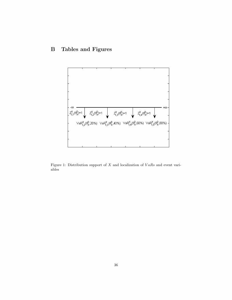
for s = 1, ...,m. For illustration, let m + 1 = 5 and suppose that the set

A = {α1, α2, α3, α4, α5} = {0%, 20%, 40%, 60%, 80%}. Figure 1 displays the

support of Xt, along with the VaRs and the event variables defining the m = 4

distinct regions.4

Now, let HXt

(θ0X

)be the vector of dimension (m, 1) with components the

m event variables

HXt

(θ0X

)=(ZXt,1

(θ0X

), ZXt,2

(θ0X

), ..., ZXt,m

(θ0X

)). (23)

We similarly define for the second time series Yt these event variables col-

4Remark that we do not consider the event variable corresponding to the extreme m + 1region identified by Xt ≥ V aRX

t,m+1

(θ0X , αm+1

). Indeed this variable is implicitly defined by

the first m event variables.

11

lected in the vector HYt

(θ0Y

), with

HYt

(θ0Y

)=(ZYt,1

(θ0Y

), ZYt,2

(θ0Y

), ..., ZYt,m

(θ0Y

)). (24)

The time series Yt does not Granger-cause the time series Xt in distribution

if the following hypothesis holds

H0 : E[HXt

(θ0X

) ∣∣FX&Yt−1

]= E

[HXt

(θ0X

) ∣∣FXt−1

]. (25)

Therefore, Granger-causality in distribution from Yt to Xt corresponds to

Granger-causality in mean from HYt

(θ0Y

)to HX

t

(θ0X

). When the null hypoth-

esis of non causality in distribution holds, this means that the event variables

defined for the variable Yt along its distribution support, do not have any predic-

tive content for the dynamics of the same event variables over the distribution

support of Xt.

Remark that our null hypothesis is flexible enough as it can be used to

check for Granger-causality in specific regions on the distribution supports, like

the center or the tails (left or right). This can be done by restricting the set

A = {α1, ..., αm+1} of VaR levels to some selected values. For instance, we

can check for Granger-causality in the left-tail distribution by setting A to

A = {0%, 1%, 5%, 10%}. In this case, the rejection of the null hypothesis is

of great importance in financial risk management, as it suggests the existence

of spill-over effects from Yt to Xt that take place in the lower tail. Similarly

Granger-causality in the center of the distribution can be checked by setting for

example A to A = {20%, 40%, 60%, 80%}. In the next subsection, we construct

a nonparametric kernel-based test statistic to test for our general null hypothesis

12

in (25), and analyze its asymptotic distribution.

2.2.2 Test statistic and asymptotic distribution

Bouhaddioui and Roy (2006) introduce a generalized portmanteau test for the

independence between two infinite order vector auto-regressive (VAR) series.

Our test statistic relies for (25) on their work. However, the asymptotic analysis

differs because (i) we are not in a VAR framework, (ii) and the events variables

ZXt,s(θ0X

)and ZYt,s

(θ0Y

)are indicator variables which are not differentiable with

respect to the unknown parameters θ0X and θ0

Y , respectively. The latter challenge

is solved relying on some asymptotic results in Hong et al. (2009).

To present the test statistic, let HXt ≡ HX

t

(θX

)and HY

t ≡ HYt

(θY

)be the estimated counterparts of the multivariate processes of event variables

HXt

(θ0X

)and HY

t

(θ0Y

), respectively, with θX and θY

√T consistent estimators

of the true unknown parameter vectors θ0X and θ0

Y . Denote Λ (j) the sample

cross-covariance matrix between HXt and HY

t , with

Λ (j) ≡

T−1

T∑t=1+j

(HXt − AX

)(HYt−j − AY

)T0 ≤ j ≤ T − 1

T−1T∑

t=1−j

(HXt+j − AX

)(HYt − AY

)T1− T ≤ j ≤ 0,

(26)

where the vector AX (resp. AY ) of length m is the sample mean of HXt (resp.

HYt ). The corresponding sample cross-correlation matrix R (j) equals

R (j) = D(

ΣX

)−1/2

Λ (j) D(

ΣY

)−1/2

, (27)

where D (.) stands for the diagonal form of a matrix, ΣX and ΣY the sample

covariance matrices of HXt and HY

t , respectively. We consider the following

13

weighted quadratic form that accounts for the dependence between the current

value of HXt and lagged values of HY

t

T =

T−1∑j=1

κ2 (j /M ) Q (j) , (28)

where κ (.) is a kernel function, M the truncation parameter and Q (j) equal to

Q (j) = Tvec(R (j)

)T (Γ−1X ⊗ Γ−1

Y

)vec

(R (j)

), (29)

with ΓX and ΓY the sample correlation matrix of HXt and HY

t , respectively.

Following Bouhaddioui and Roy (2006), our test statistic is a centered and scaled

version of the quadratic form in (28), i.e.,

VY→X =T −m2CT (M)

(m2DT (M))1/2

, (30)

with CT (M) and DT (M) as defined in (19) and (20) respectively. The above

test statistic generalizes in a multivariate setting the one in Hong et al. (2009).

Indeed when m is equal to one, which corresponds to the univariate case where

each of the vectors HXt and HY

t has only one event variable, the test statistic

VY→X in (30) is exactly equal to the Hong et al. (2009) test statistic in (18).

The following proposition gives the asymptotic distribution of our test statistic.

Proposition 1 Suppose that Assumptions of Theorem 1 in Hong et al. (2009)

hold. Then under the null hypothesis of no Granger-causality in distribution as

stated in (25), we have

VY→X =T −m2CT (M)

(m2DT (M))1/2−→d N (0, 1) .

14

Assumptions of Theorem 1 in Hong et al. (2009) impose some regulatory

conditions on the time series Xt and Yt, on the VaR models used including

smoothness, moment conditions and adequacy, on the kernel function κ (.), and

also on the truncation parameter M . The latter should be equal to M = cT v

with 0 < c <∞, 0 < v < 1/2, v < min(

2d−2 ,

3d−1

)if d ≡ max (dX , dY ) > 2 and

dX (resp. dY ) is the dimension of the parameter θX (resp. θY ). See Hong et al.

(2009, pp. 275) for a complete discussion on these assumptions.

The proof of Proposition 1 proceeds as follows. Consider the following de-

composition of our test statistic

VY→X =T ∗ −m2CT (M)

(m2DT (M))1/2

+T − T ∗

(m2DT (M))1/2

, (31)

with T ∗ the pseudo version of the weighted quadratic form in (28-29) computed

using the true correlation matrices ΓX and ΓY , i.e.,

T ∗=T−1∑j=1

κ2 (j /M ) Q∗ (j) , (32)

Q∗ (j) = Tvec(R (j)

)T (Γ−1X ⊗ Γ−1

Y

)vec

(R (j)

). (33)

Under the decomposition in (31), the proof of Proposition 1 is given by the

following two lemmas:

Lemma 2 Under Assumptions of Theorem 1 in Hong et al. (2009), we have

T ∗ −m2CT (M)

(m2DT (M))1/2−→d N (0, 1) . (34)

Lemma 3 Under Assumptions of Theorem 1 in Hong et al. (2009), we have

T − T ∗

(m2DT (M))1/2−→p 0. (35)

The proofs of these two Lemmas are reported in Appendix A.

15

3 Small sample properties

In this section, we study the finite sample properties of our test via Monte Carlo

simulation experiments. We analyze the size in the first part of the section and

the remaining one is devoted to the analysis of the power.

3.1 Empirical size analysis

We simulate the size of the nonparametric test of Granger-causality test in

distribution assuming the following data generating process (DGP) for the first

time series Xt: Xt = σtvt,

σ2t = 0.1 + 0.5σ2

t−1 + 0.2X2t−1,

vt ∼ m.d.s. (0, 1) ,

which corresponds to a GARCH(1,1) model. We make the assumption that the

second time series Yt follows the same process. Because the two processes are

generated independently, there is no Granger causality in distribution between

them. For a given value of the sample size T ∈ {500, 1.000, 2.000}, and for each

simulation, we compute our test statistic in (30) and make inference using the

asymptotic Gaussian distribution. For the computation of the test statistic, we

need to specify a model to estimate the VaRs (at the risk level α1, ..., αm+1)

and the m event variables for each variable Xt and Yt. The m + 1 VaRs are

computed using a GARCH(1,1) model estimated by quasi-maximum likelihood.

The estimated values of the m+ 1 VaRs at time t are

V aRXt,s = σt,Xq (vt, αs) , s = 1, ...,m+ 1, (36)

16

where σt,X is the fitted volatility at time t, and q (vt, αs) the empirical quantile

of order αs of the estimated standardized innovations. We proceed similarly

to compute the m + 1 VaRs and the corresponding m event variables for the

second time series Yt. Note that we set the parameter m+ 1 to 14 and the set

A to A = {α1, α2, ..., α14} = {0%, 1%, 5%, 10%, 20%, ..., 90%, 95%, 99%}, which

covers regions in the tails and the center of the distribution support of each

time series.5 We also need to make a choice about the kernel function in order

to compute our test statistic. We consider the four different usual kernels, i.e.

The Daniell (DAN), the Parzen (PAR), the Bartlett (BAR) and the Truncated

uniform (TR) one.

Lastly for the choice of the truncation parameter M , we use three different

values: M = [ln (T )], M =[1.5T 0.3

]and M =

[2T 0.3

], with [.] the integer part

of the argument. These rates lead to the values M = 6, 10, 13 for T = 500,

M = 7, 12, 16 for T = 1.000, and M = 8, 15, 20 for T = 2.000. These values

cover a range of lag orders for the sample sizes considered. Table 1 displays the

empirical sizes of our test over 500 simulations and for two different nominal

risk levels η ∈ (5%, 10%). Results in Table 1 show that our test is well-sized.

Indeed, the rejection frequencies are close to the nominal risk levels. Hence, the

standard Gaussian distribution provides asymptotically a good approximation

of the distribution of our test statistic. This result seems to hold regardless of

the kernel function used and the value of the truncation parameter M .

5Recall that for αs = 0%, the VaR corresponds to −∞.

17

3.2 Empirical power analysis

We now simulate the empirical power of our test. Since causality in distribution

springs from causality in moments such as mean or variance, we assume different

DGPs which correspond to these cases. The first DGP assumes the existence of a

linear Granger-causality in mean in order to generate data under the alternative

hypothesis: Yt = 0.5Yt−1 + ut,Y ,

ut,Y = σt,Y vt,Y ,

σ2t,Y = 0.1 + 0.5σ2

t−1,Y + 0.2u2t−1,Y ,

(37)

Xt = 0.5Xt−1 + 0.3Yt−1 + ut,X ,

ut,X = σt,Xvt,X ,

σ2t,X = 0.1 + 0.5σ2

t−1,X + 0.2u2t−1,X ,

(38)

where both vt,Y and vt,X are martingale difference sequences with mean 0 and

variance 1. The empirical powers of our test are computed over 500 simulations

for T ∈ {500, 1.000, 2.000}. As in the analysis of the size, we consider three

values of the truncation parameter M, and two nominal risk levels η = 5%, 10%.

The results are reported in Table 2, only for the Daniell kernel to save space.6

For comparison we also display in Table 2 results for the Granger-causality

test in mean. In order to have a fair comparison, we do not use the usual

parametric Granger-causality test in mean derived from a vector autoregressive

model. We consider instead the kernel-based non-parametric Granger-causality

test in mean introduced by Hong (1996). Results in Table 2 show that our kernel-

based nonparametric test for Granger-causality in distribution has appealing

6Results for the other kernels are similar and available from the authors upon request. Theonly exception occurs for the uniform kernel which has a relatively low power, because of itsuniform weighting which does not discount higher order lags.

18

power properties. For instance, the rejection frequencies of the null hypothesis

for (T,M) = (500, 6) are equal to 93.6% and 95.6% for η = 5% and 10%,

respectively. For T = 1.000, 2.000 the powers are equal to one. The rejection

frequencies of the Granger-causality test in mean are always equal to 100%

and hence are slightly higher than the ones of our Granger-causality test in

distribution for the smallest sample. This result is expected as the assumed

causality in distribution springs from causality in mean.

To stress the relevance of our testing approach, we consider a second repre-

sentation of the DGPs under the alternative hypothesis, assuming causality in

distribution stemming from a non-linear form of causality in mean. Precisely,

we generate data for the time series Yt using the specification in (37), and the

second time series is generated as followsXt = 0.5Xt−1 + 0.3Y 2

t−1 + ut,X ,

ut,X = σt,Xvt,X ,

σ2t,X = 0.1 + 0.5σ2

t−1,X + 0.2u2t−1,X .

(39)

Table 3 reports the rejection frequencies over 500 simulations. The presen-

tation is similar to Table 2. We observe that while the Granger-cauality test

in mean fails to reject the null hypothesis for most of the simulations, our test

still exhibits good power in detecting this non-linear form of causality. For il-

lustration the rejection frequency of the null hypothesis for (T,M) = (500, 6) is

equal to 75.2% for η = 5%, while it is only equal to 18.2% for the causality test

in mean in the same configuration. Remark that for our test, the power drops

as the truncation parameter M increases. Moreover, the power increases as the

sample size increases and converges to 100%.

19

Lastly, we generate data under the alternative hypothesis, assuming Granger-

causality in variance. Formally, we suppose once again that Yt has the specifi-

cation in (37), and Xt is generated asXt = 0.5Xt−1 + ut,X ,

ut,X = σt,Xvt,X ,

σ2t,X = 0.1 + 0.5σ2

t−1,X + 0.2u2t−1,X + 0.7Y 2

t−1.

(40)

Results displayed in Table 4 are qualitatively similar to the ones in Table

3. Our causality test in distribution has good powers in rejecting the null

hypothesis, while the causality test in mean exhibits low powers. Overall the

reported values are lowers to the ones in Tables 2 and 3. This pattern can be

explained by the fact that (i) causality in variance takes place mainly in the

tails, (ii) and the dynamics of the tails are more difficult to fit due to the lack

of data.

4 Empirical part

Recent financial crises have all been characterized by quick and large regional

spill-overs of negative financial shocks. For example, consecutively to the Greek

distress, South European countries have been contaminated, facing skyrocketing

refinancing rates. Besides it has impacted North European states in an oppo-

site way. Considered as safe harbors for investors, they were able to refinance

their debt on markets at lower rates. It is obvious that the degree of globaliza-

tion within European Union as well as the low degree of fiscal federalism has

fostered the speed as well as the amplitude of the transmission mechanism of

such a shock. And as Southern European countries used foreign capital markets

20

to finance their domestic investments and boost their growth, they have been

highly subject to financial instability.

It is of major importance for empirical studies to evaluate the importance of

these spill-overs. Theoretically it relies on the crisis-contingent theories, which

explain the increase in market cross-correlation after a shock issued in an ori-

gin country as resulting from multiple equilibria based on investor psychology;

endogenous liquidity shocks causing a portfolio recomposition; and/or political

disturbances affecting the exchange rate regime.7 8 The presence of spill-overs

during a crisis can be thus tested empirically by a significant and transitory in-

crease in cross-correlation between markets. (See inter alia King and Wadhwani,

1990, Calvo and Reinhart, 1995 and Baig and Goldfajn, 1998). Nevertheless,

this intuitive approach, which presents the advantage of simplicity as it avoids

the identification of the transmission channels, presents many shortcomings:

First, Forbes and Rigobon (2002) show that an increase in correlation can

be exclusively driven by an higher volatility during crisis periods. In such a

case, it could not be attributed to a stronger economic interdependence. To

correct for this potential bias, they thus propose to use a modified version of

the correlation9 and test for its temporary increase during crisis period.

Second, correlation is a symmetrical measure: an increase in the correlation

between markets i and j does not provide any information on the direction of

the contagion (from i to j, from j to i, or both). For such a reason, Bodart and

7see Rigobon (2000) for a survey.8On contrary, according to the non-crisis-contingent theories, the propagation of shocks

does not lead to a shift from a good to a bad equilibrium, but the increase in cross-correlationis the continuation of linkages (trade and/or financial) existing before the crisis.

9In fact, they are using the unconditional correlation instead of the conditional one.

21

Candelon (2009) prefer to consider an indicator of causality to measure spill-

overs. It is thus possible to evaluate asymmetrical spill-overs, which can then

move from i to j, j to i or in both direction. Besides, using Granger-causality

approach requires the estimation of multivariate dynamic models which are less

prone to potential misspecification issues.

It is, more or less, feasible to tackle both these shortcomings in a classical

framework. Nevertheless, even if comparing causality between pre- and crisis

periods allows to evaluate spill-overs, it does not permit to separate interde-

pendence and contagion. Interdependence deals with the long run structural

links between markets. It thus provides information on the extend to which

markets are integrated. Therefore, interdependence should be analysed without

considering extreme positive or negative events. On the contrary, contagion

deals with short-run abrupt increases in the causal linkages and takes place

exclusively during crisis’ period. Thus, testing for contagion requires to exclu-

sively focus on the extremal left tail of the distribution, as it is performed in

extreme value theory (see Hartman et al., 2004). Our Granger-causality test

in distribution allows to tackle all these issues. Indeed, it offers an asymmetric

measure of spill-overs, based on a dynamic representation. Besides, it is possible

to investigate if causality has increased for the whole distribution but also for

specific percentiles of the distribution, in particular those located at the left tail

or right tails, corresponding to extreme events.

As an illustration, we analyse the recent European crisis and consider a set

of 12 European daily stock market indices (Austria, Belgium, Finland, France,

22

Germany, Greece, Ireland, Italy, Luxemburg, the Netherlands, Portugal and

Spain) downloaded from datastream ranging from January 1, 2007 to May 6,

2011 (i.e. T = 1.134 observations). The first empirical illustration consists in

testing for interdependence. It is performed implementing the pairwise Granger-

causality for the whole distribution but removing crisis’s periods, i.e. the right

and left tails. Then, in a second analysis, we repeat this analysis for the left

tail in order to test for contagion during crisis. This part refers to the EVT

approach of spill-overs and extend the Hartmann et al (2004). Similarly, the

test is conducted for the right tail, i.e. upswing period. We can then compare

the strength of contagion during crises vs boom periods and check in which

periods contagion is the most significant.

4.1 The general design of the Granger-causality test indistribution to test for spill-over

To implement the Granger-causality test in distribution in our empirical illustra-

tion, we first need to compute for each index, m+1 series of VaRs corresponding

to m+ 1 risk level αs s = 1, ...,m+ 1, which cover its distribution support. As

for the Monte Carlo simulations, we consider the following set for the VaR levels

A = {0%, 1%, 5%, 10%, ..., 90%, 95%, 99%} with m + 1 = 14. To compute the

VaRs, we use a semi-parametric model. Formally, we suppose that each index

returns series Ri,t i = 1, ..., 12, follows an AR (m)-GARCH (p, q) model, with:

Ri,t =∑m

j=1φi,jRi,t−j + εi,t, (41)

εi,t = σi,tvi,t, (42)

23

σ2i,t = κi +

∑q

j=1γi,jε

2i,t−j +

∑p

j=1βi,jσ

2i,t−j , (43)

and vi,t an i.i.d. innovation with mean zero and unit variance. The choice for an

AR (m)-GARCH (p, q) is in line with the Forbes and Rigobon (2002) correction.

It accounts for volatility increase that biases the causality analysis. For each

index, this model is estimated by quasi-maximum likelihood method. Hence,

the m+ 1 series of VaRs are obtained as:

V aRit,s =∑m

j=1φi,jRi,t−j + σt,iq (vi,t, αs) , s = 1, ...,m+ 1, (44)

with σt,i the fitted volatility at time t for the index number i, and q (vi,t, αs)

the empirical quantile of order αs of the estimated standardized innovations vi,t.

Table 5 displays the estimation results of the AR(m)-GARCH(p, q) models for

the indices. As shown through the Ljung-Box test applied to the residuals and

their squares, the retained specifications successfully capture the dependence in

the first two moments.

With the fitted series of VaRs at hand, we calculate for each index, the

multivariate process of dynamic inter-quantiles events variables, and compute

for each couple (i, j) of indices our kernel-based non parametric test statistic

Vj→i as defined in (30). For the computation we use the Daniell kernel and set

the truncation parameter M to[1.5T 0.3

]which leads to the value of M = 12

for the whole sample of length T = 1.134.

4.2 Testing for interdependence

To test for interdependence, we follow the general design of the pairwise test of

Granger-causality in distribution as described above except that we remove from

24

the distribution the extreme events. The new set A of VaRs risk levels is equal to

A = {20%, 30%, ..., 70%, 80%} with m+1 = 7. Table 6 displays the results of the

test. The reported values are the p-values in percentage. Hence, for a nominal

risk level of 5%, we reject the null hypothesis of no-causality from index j to

index i when the reported value is lower than 5%. Test statistics corresponding

to the rejection of the null hypothesis of no causality are put in bold. The

last column labelled ”Sum” provides for a given index in row, the number of

time it is Granger-caused by the others. Similarly, the last row labelled ”Sum”

provides for a given stock market index the number of time it Granger-causes

others stock market indices. Lastly, the entry corresponding to the last row

and last column gives the total number of significant Granger-causality cases

for our set of indices. It turns out that interdependence is supported in only

9.8% of the cases (13 cases out of 132). This result indicates that European

stock market integration is far from being achieved. Looking at the countries

results, we observe that the Austrian and the French stock markets are the most

integrated ones, as they are affected by 3 other European markets, respectively.

On the contrary, Greece, Ireland, Italy, Luxemburg and Netherlands appear as

independent from the other markets. It is interesting to notice that the causal

matrix is not symmetric: France which is among the most caused markets does

not affect any market. It hence supports our choice for causality as a measure

of spill-over rather than correlation. The most causal markets are Netherlands,

Greece and Portugal. The presence of these two last countries is interesting

as they were among the main drivers of the European crisis. Their causal

25

importance, which can be qualified as systemic for the rest of Europe, should

have constituted a signal of alarm at the edge of the crisis.

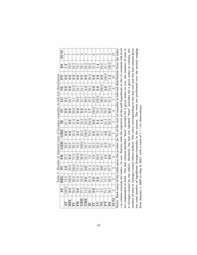
4.3 Testing for contagion

Contagion is apprehended implementing our Granger-causality test in left-tail

distribution. The set A of VaRs risk levels is now set as A = {0%, 1%, 5%, 10%}

with m + 1 = 4. Table 7 displays the outcomes of the tests. The number

of causal pairs increases to 35.6% of the cases supporting hence the presence

of contagion. We observe that the most causal markets are Portugal, Italy,

Netherlands, Greece and Ireland, and except Netherlands, this group includes

all the countries in turmoils (Portugal, Italy, Greece and Ireland), around which

the crisis was build. On the other side, the most caused markets are Austria,

Belgium, Italy, France, Luxembourg and Greece. Remark the predominant role

of Italy and Greece in the system, which cause and are caused in many cases.

The Granger-causality test is now repeated for the left-tail distribution with

A = {90%, 95%, 99%, 100%}, i.e., m + 1 = 4 and results are reported in Table

8. It appears that ”positive” contagion is only supported in 7.5% of the cases

and concerns mainly Spain as spill-overs driver, and Luxembourg, Germany

and Belgium as spill-overs receivers. The asymmetry between causal tests in the

right and left tail is striking. Whereas spill-overs are important in crisis periods,

they are only weakly present in upswing times. Such a feature highlights that

European stock markets integration is strongly vulnerable to negative, and to

a lesser extend positive, shocks. European policy makers should acknowledge it

and set up structural measures to limit it.

26

5 Conclusion

A kernel-based non-parametric test for Granger-causality in distribution be-

tween two time series is proposed in this paper. The test checks for spill-overs

between the multivariate processes of dynamics inter-quantile event variables as-

sociated to each variable. Beyond the existing approaches our testing approach

has two main advantages. First, it can be used to test for Granger-causality in

specific regions of the distributions, like the center or the tails (left and right).

Second, it checks for a large number of lags discounting higher order lags, and

hence is consistent against causality which carries over long distributional lags.

We show that the test has a standard Gaussian distribution under the null

hypothesis which is free of parameter estimation uncertainty. We run a Monte

Carlo simulations exercise which shows that the Gaussian distribution is valid

in small samples. The test also has very appealing power properties in vari-

ous settings including linear and non-linear causality in mean and causality in

variance.

In an empirical part we implement our testing procedure to 12 European

daily stock market indices to analyze spill-overs during the recent European

crisis. As our test is designed to check for causality in specific regions of the

distribution (center or tails), it can be used to test for both the presence of

interdependence and contagion. Indeed interdependence can be checked through

Granger-causality in the center of the distribution, as interdependence is a long

run path that takes place in normal periods. On the contrary, contagion refers

to a short-run abrupt increase in the causal linkages taking place exclusively

27

during crisis period, and can be tested via Granger-causality in distribution’s

tails.

The empirical results indicate that European stock market integration is far

from being achieved, because we observe very weak evidence supporting inter-

dependence. On contrary, our results support the presence of contagion, with a

strong asymmetry between contagion in the right and left tails. More precisely,

contagion is important in crisis periods, whereas it is weak in upswing times.

Such a result constitutes an important feature for the European stock markets,

and policy makers should acknowledge it in designing structural measures for

financial stability.

A Proof of LEMMAS

A.1 Proof of LEMMA 2

Lemma 2: Under Assumptions of Theorem 1 in Hong et al. (2009), we have

T ∗ −m2CT (M)

(m2DT (M))1/2−→d N (0, 1) . (45)

Proof: Consider the pseudo version of the weighted quadratic form T ∗ de-

fined as

T ∗=T−1∑j=1

κ2 (j /M ) Q∗ (j) , (46)

Q∗ (j) = Tvec(R (j)

)T (Γ−1X ⊗ Γ−1

Y

)vec

(R (j)

), (47)

where ΓX (resp. ΓY ) is the correlation matrix of the true unknown multivariate

process of event variables HXt

(θ0X

)(resp. HY

t

(θ0Y

)). Recall that HX

t

(θ0X

)is

defined as

HXt

(θ0X

)=(ZXt,1

(θ0X

), ..., ZXt,m

(θ0X

)), (48)

28

where the event variables ZXt,s(θ0X

), s = 1, ...,m, are related to distinct regions

on the distribution support of Xt. Hence, they are mutually independent, and

the associated correlation matrix ΓX is equal to the identity matrix. The same

reasoning applies for HYt

(θ0Y

), with the consequence that ΓY is also equal to

the identity matrix. Hence, the pseudo weighted quadratic form T ∗ defined in

(46-47) takes the expression

T ∗ = T

T−1∑j=1

κ2 (j /M ) vec(R (j)

)Tvec

(R (j)

). (49)

Since R (j) is defined as the cross-correlation matrix at lag-order j between

HXt =

(ZXt,1, ..., Z

Xt,m

)and HY

t =(ZYt,1, ..., Z

Yt,m

), its components are given by

the correlations between ZXt,k and ZYt−j,p with k = 1, ...m and p = 1, ...,m. Let

us denote ρk,p (j) such correlation, i.e.,

ρk,p (j) = corr(ZXt,k, Z

Yt−j,p

). (50)

With the definition of the vec operator, it is easy to see that vec(R (j)

)has

m2 components given by ρk,p (j), k = 1, ...m and p = 1, ...,m. Consequently,

the pseudo quadratic form T ∗ in (49) becomes

T ∗ = T

T−1∑j=1

κ2 (j /M )

m∑k=1

m∑p=1

ρ2k,p (j) ,

=

m∑k=1

m∑p=1

T T−1∑j=1

κ2 (j /M ) ρ2k,p (j)

. (51)

For a given value of the couple (k, p), the quadratic form in the bracket of (51)

corresponds to the uncentered and unscaled test statistic in Hong et al. (2009)

for the Granger-causality from ZYt,p to ZXt,k, and these statistics are obviously

29

independent. We deduce from this that under Assumptions of Theorem 1 in

Hong et al. (2009)

T

T−1∑j=1

κ2 (j /M ) ρ2k,p (j)−→d N (CT (M) , DT (M)) . (52)

Remark that the event variables in Hong et al. (2009) are related to one-

sided regions, whereas we have to deal with two-sided regions in our framework.

However in their proof of Theorem 1, it is easy to see that all of the technical

results remain valid even in the case of two-sided regions. For this, it suffices

to replace Z1t (θ1) and Z2t (θ2) by ZXt,k (θX) and ZYt,p (θY ), with θX and θY

any vector in the parameter spaces ΘX and ΘY , respectively. Moreover, the

martingale difference sequence W1t (θ1) and W2t (θ2) in the proof of Theorem 1

in Hong et al. (2009) must be replaced by WXt,k (θX) and WY

t,p (θY ) respectively

in order to deal with two-sided regions, with

WXt,k (θX) = ZXt,k (θX)− ZXt,k

(θ0X

)− E

(ZXt,k (θX)

∣∣FXt−1

)+ E

(ZXt,k

(θ0X

) ∣∣FXt−1

)= ZXt,k (θX)− ZXt,k

(θ0X

)−[FX(V aRXt,k+1 (θX)

)− FX

(V aRXt,k (θX)

)]+

+[FX(V aRXt,k+1

(θ0X

))− FX

(V aRXt,k

(θ0X

))],

WYt,p (θY ) = ZYt,p (θY )− ZYt,p

(θ0Y

)− E

(ZYt,p (θY )

∣∣FYt−1

)+ E

(ZYt,p

(θ0Y

) ∣∣FYt−1

)= ZYt,p (θY )− ZYt,p

(θ0Y

)−[FY(V aRYt,p+1 (θY )

)− FY

(V aRYt,p (θY )

)]+

+[FY(V aRYt,p+1

(θ0Y

))− FY

(V aRYt,p

(θ0Y

))],

with FX(.) and FY (.) the conditional cumulative distribution functions of X and

Y respectively. Hence, we can conclude using (52) that the pseudo quadratic

30

form T ∗ in (51) has the limiting distribution

T ∗−→d N(m2CT (M) ,m2DT (M)

). (53)

and this completes the proof of LEMMA 2.

A.2 Proof of LEMMA 3

Lemma 3: Under Assumptions of Theorem 1 in Hong et al. (2009), we have

T − T ∗

(m2DT (M))1/2−→p 0. (54)

Proof: The proof of Lemma 3 proceeds by combining elements in the proofs

of Proposition 3.2 in Bouhaddioui and Roy (2006) and Theorems A.1 and A.3

in Hong et al. (2009). Formally, given that

DT (M) = M

∫ ∞0

κ4 (z) dz [1 + o (1)] , (55)

as M →∞, the proof of Lemma 3 can be established showing that

T − T ∗ = Op

(M/T 1/2

). (56)

Based on Lemma 4.1 in El Himdi and Roy (1997), the quadratic forms T

and T ∗ can be rewritten in term of cross-covariances as

T = T

T−1∑j=1

κ2

(j

M

)vec

(Λ (j)

)T (Σ−1X ⊗ Σ−1

Y

)vec

(Λ (j)

), (57)

T ∗ = T

T−1∑j=1

κ2

(j

M

)vec

(Λ (j)

)T (Σ−1X ⊗ Σ−1

Y

)vec

(Λ (j)

), (58)

with Λ (j) the sample cross-covariance matrix at lag-order j, ΣX and ΣY the co-

variance matrices of the true multivariate processes of event variables HXt

(θ0X

)31

and HYt

(θ0Y

), and ΣX and ΣY their sample counterparts given by the covari-

ance matrices of HXt ≡ HX

t

(θX

)and HY

t ≡ HYt

(θY

), respectively. It follows

that

T − T ∗ = T

T−1∑j=1

κ2

(j

M

)vec

(Λ (j)

)T {Σ−1X ⊗ Σ−1

Y − Σ−1X ⊗ Σ−1

Y

}vec

(Λ (j)

).

(59)

Now, let us study the asymptotic behavior of ΣX . The components of this

matrix are given by the covariance between the estimated event variables ZXt,k,

k = 1, ...,m. Let Ck,p be a typical element of ΣX with

Ck,p = cov(ZXt,k, Z

Xt,p

). (60)

Let C0k,p be the true value of Ck,p, i.e., the covariance between the true event

variables ZXt,k(θ0X

)and ZXt,p

(θ0X

). Note that C0

k,p is a typical element of ΣX .

The difference between Ck,p and C0k,p can be decomposed as follows

Ck,p − C0k,p = M1

(θX

)+ M2

(θX

)+ M3

(θX

), (61)

with

M1

(θX

)= T−1

T∑t=1

[ZXt,k − ZXt,k

(θ0X

)] [ZXt,p

(θ0X

)− πXp

](62)

M2

(θX

)= T−1

T∑t=1

[ZXt,k

(θ0X

)− πXk

] [ZXt,p − ZXt,p

(θ0X

)](63)

M3

(θX

)= T−1

T∑t=1

[ZXt,k − ZXt,k

(θ0X

)] [ZXt,p − ZXt,p

(θ0X

)], (64)

where we replace the sample means πXk and πXp of Zt,k and Zt,p by their true

respective values πXk = E(ZXt,k

(θ0X

))and πXp = E

(ZXt,p

(θ0X

)). Using the fol-

32

lowing result in the proof of theorem A.3 in Hong et al. (2009)

supθX∈ΘX

∣∣∣M1 (θX)∣∣∣ = Op

(T−1/2

), (65)

with θX any√T -consistent estimator of θ0

X in the space ΘX , we have for the

first term

M1

(θX

)= Op

(T−1/2

). (66)

Similar arguments apply for the last two terms, with the consequence that

M2

(θX

)= Op

(T−1/2

), (67)

M3

(θX

)= Op

(T−1/2

). (68)

We deduce that

Ck,p − C0k,p = Op

(T−1/2

), (69)

and

ΣX − ΣX = Op

(T−1/2

). (70)

Using the same reasoning for the elements of ΣY we have that

ΣY − ΣY = Op

(T−1/2

), (71)

and

Σ−1X ⊗ Σ−1

Y − Σ−1X ⊗ Σ−1

Y = Op

(T−1/2

). (72)

Hence equation (59) becomes

T − T ∗ = T

T−1∑j=1

κ2

(j

M

)vec

(Λ (j)

)TOp

(T−1/2

)vec

(Λ (j)

)(73)

= Op

(T 1/2

) T−1∑j=1

κ2

(j

M

)vec

(Λ (j)

)Tvec

(Λ (j)

).

33

The rest of the proof proceeds by showing that

B (T ) =

T−1∑j=1

κ2

(j

M

)vec

(Λ (j)

)Tvec

(Λ (j)

)= Op (M/T ) . (74)

We decompose B (T ) into two parts

B (T ) = B1 (T ) + B2 (T ) , (75)

with

B1 (T ) =

T−1∑j=1

κ2

(j

M

){vec

(Λ (j)

)Tvec

(Λ (j)

)− vec (Λ (j))

Tvec (Λ (j))

},

(76)

B2 (T ) =

T−1∑j=1

κ2

(j

M

)vec (Λ (j))

Tvec (Λ (j)) , (77)

where Λ (j) is the cross-covariance matrix at lag-order j of the true event vari-

ables HXt

(θ0X

)and HY

t

(θ0Y

). Let us first consider B1 (T ) in (76). Since Λ (j)

is defined as the estimated cross-covariance matrix at lag-order j between

HXt =

(ZXt,1, Z

Xt,2, ..., Z

Xt,m

), (78)

and

HYt =

(ZYt,1, Z

Yt,2, ..., Z

Yt,m

), (79)

its components are given by the covariances between ZXt,k and ZYt−j,p, k =

1, ...,m, p = 1, ...,m. Denote Ck,p (j) such covariances. Using the definition

of the vec operator we thus have

B1 (T ) =

T−1∑j=1

κ2

(j

M

) m∑k=1

m∑p=1

{C2k,p (j)− C2

k,p (j)}, (80)

34

which can be rewritten as

B1 (T ) =

T−1∑j=1

κ2

(j

M

) m∑k=1

m∑p=1

{(Ck,p (j)− Ck,p (j)

)2

+(Ck,p (j)− Ck,p (j)

)Ck,p (j)

}

=

m∑k=1

m∑p=1

{Q1 + Q2

}, (81)

with

Q1 =

T−1∑j=1

κ2

(j

M

)(Ck,p (j)− Ck,p (j)

)2

, (82)

Q2 =

T−1∑j=1

κ2

(j

M

)(Ck,p (j)− Ck,p (j)

)Ck,p (j) . (83)

Using the results of Theorem A.1 in Hong et al. (2009), that is

Q1 = Op

(M1/2/T

), (84)

Q2 = Op

(M1/2/T

), (85)

we have

B1 (T ) = Op

(M1/2/T

). (86)

For the second term B2 (T ), using the Markov inequality, we have

B2 (T ) =

T−1∑j=1

κ2

(j

M

)vec (Λ (j))

Tvec (Λ (j)) = Op (M/T ) . (87)

We deduce from (86) and (87) that

B (T ) = Op (M/T ) , (88)

and

T − T ∗ = Op

(T 1/2

)Op (M/T ) = Op

(M/T 1/2

). (89)

This completes the proof of Lemma 3.

35

B Tables and Figures

Figure 1: Distribution support of X and localization of V aRs and event vari-ables

36

Table 1: Empirical sizes of the Granger-causality test in distribution

T M η DAN BAR PAR TR

6 5% 5.80 5.80 5.60 4.40

10% 10.40 10.40 11.40 9.80

500 10 5% 5.20 5.60 5.80 5.60

10% 10.00 9.60 10.20 11.60

13 5% 5.60 4.80 5.20 5.40

10% 10.40 10.60 10.20 11.80

7 5% 5.00 4.20 4.40 5.20

10% 9.00 9.40 8.40 10.80

12 5% 5.00 5.20 5.00 6.00

1000 10% 9.40 10.00 9.00 11.80

16 5% 5.40 5.60 6.20 6.20

10% 10.00 10.20 10.00 11.40

8 5% 6.60 7.00 6.60 5.20

10% 11.80 11.80 13.40 8.80

15 5% 5.60 6.20 6.40 6.20

2000 10% 10.20 11.20 11.60 11.60

20 5% 5.00 5.00 6.60 4.80

10% 10.60 10.80 11.20 9.60

Notes: The table displays the empirical sizes (in %) of the Granger-causality

test in distribution. Rejection frequencies are reported over 500 simulations

for two nominal risk levels η, with T the sample size and M the truncation

parameter. DAN, BAR, PAR and TR refer to the Daniell, the Bartlett, the

Parzen, and the truncated kernels, respectively.

37

Table 2: Empirical powers of the Granger-causality test in distri-bution: DGP1T M η Distribution Mean

6 5% 93.60 100.00

10% 95.60 100.00

500 10 5% 91.80 100.00

10% 93.20 100.00

13 5% 90.40 100.00

10% 92.40 100.00

7 5% 100.00 100.00

10% 100.00 100.00

12 5% 100.00 100.00

1000 10% 100.00 100.00

16 5% 100.00 100.00

10% 100.00 100.00

8 5% 100.00 100.00

10% 100.00 100.00

15 5% 100.00 100.00

2000 10% 100.00 100.00

20 5% 100.00 100.00

10% 100.00 100.00

Notes: The table displays the empirical powers (in %) of the

Granger-causality test in distribution. Rejection frequencies are

reported over 500 simulations for two nominal risk levels η, with

T the sample size and M the truncation parameter. For compar-

ison, we also report the rejection frequencies of the kernel-based

nonparametric test in mean. For both test, results are reported

for the Daniell kernel. Data are generated under the alternative

hypothesis assuming Granger-causality in mean.

38


6 5% 75.20 18.20

10% 82.80 21.40

500 10 5% 68.20 16.20

10% 76.60 20.60

13 5% 60.20 15.80

10% 70.60 20.60

7 5% 97.80 20.60

10% 98.40 21.60

12 5% 95.80 19.20

1000 10% 97.00 23.20

16 5% 93.00 19.20

10% 95.80 22.60

8 5% 100.00 24.20

10% 100.00 28.60

15 5% 100.00 19.60

2000 10% 100.00 24.40

20 5% 100.00 17.60

10% 100.00 21.80








hypothesis assuming nonlinear Granger-causality in mean.

39


6 5% 51.40 18.80

10% 61.40 23.00

500 10 5% 50.20 20.40

10% 60.40 25.80

13 5% 48.20 21.40

10% 57.80 25.80

7 5% 79.80 17.80

10% 86.80 21.60

12 5% 72.40 22.60

1000 10% 81.60 27.40

16 5% 67.00 21.80

10% 76.20 29.00

8 5% 99.20 15.40

10% 99.40 19.40

15 5% 96.60 18.80

2000 10% 97.60 23.40

20 5% 93.00 19.00

10% 95.80 24.40








hypothesis assuming Granger-causality in variance.

40

Table 5: Estimation results of AR-GARCH modelsIndex φi,1 κi γi,1 γi,2 γi,3 βi,1 LBvi,t (6) LBv2i,t (6)

AT 0.000(4.148)

0.150(7.752)

0.839(44.371)

5.217 1.840

BEL 0.000(5.597)

0.137(10.559)

0.839(63.863)

4.738 2.857

FI 0.000(3.590)

0.081(8.170)

0.907(75.696)

5.750 0.758

FR 0.000(4.310)

0.127(8.340)

0.857(50.623)

3.445 7.400

GER 0.000(4.568)

0.117(7.773)

0.863(50.254)

3.717 6.317

GRE 0.072(2.184)

0.000(3.057)

0.116(7.549)

0.881(62.744)

10.665 8.400

IE 0.000(3.792)

0.131(6.687)

0.853(40.945)

7.161 1.985

IT 0.000(4.670)

0.000(0.000)

0.179(4.831)

0.797(34.446)

3.523 5.840

LU 0.000(3.289)

0.081(9.318)

0.912(96.818)

2.789 1.073

NL 0.000(4.574)

0.129(8.913)

0.854(56.663)

4.441 3.166

PT 0.000(4.185)

0.183(8.490)

0.800(39.230)

5.986 1.622

ES 0.000(5.356)

0.058(1.787)

0.034(0.799)

0.160(4.377)

0.708(21.312)

3.374 9.580

Notes: For each index, the Table displays the estimation results of the AR-GARCH model

in equations (41-43). We report the parameters estimates followed in brackets by the

student statistics. The two last columns give the results of the Ljung-Box test applied to

the serie of the standardized innovations vi,t and its square, respectively, with 6 the number

of lags. The critical value for the rejection of the null hypothesis at the 5% nominal risk

level is equal to 12.59.

41

Tab

le6:

Res

ult

sof

bil

ater

alte

sts

of

Gra

nger

causa

lity

inth

ece

nte

rof

the

dis

trib

uti

on

AT

BEL

FI

FR

GER

GRE

IEIT

LU

NL

PT

ES

SUM

AT

100.0

2.3

27.1

14.0

27.

038.

979.1

2.7

48.2

1.0

19.

729.

63

BEL

0.5

100.0

27.6

19.9

64.

453.

94.2

5.3

18.3

31.5

85.

66.4

2FI

80.9

98.3

100.0

10.4

90.

822.

621.0

70.2

60.1

79.8

21.

83.7

1FR

42.0

28.0

38.6

100.0

8.2

0.0

39.4

10.2

2.6

58.3

0.1

44.

73

GER

95.9

26.1

27.4

8.6

100.0

0.2

36.9

98.4

5.1

16.3

14.

098.

41

GRE

54.1

47.3

28.7

50.7

60.

6100.0

28.3

30.3

55.6

92.1

72.

870.

20

IE42.4

59.6

5.2

11.8

15.

790.

6100.0

15.9

25.4

85.6

23.

442.

60

IT65.0

42.6

80.9

72.9

9.6

46.

277.3

100.0

45.3

44.0

46.

491.

90

LU

37.6

97.7

65.3

7.2

12.

091.

629.7

30.7

100.0

95.0

48.

311.

00

NL

94.9

99.3

75.4

15.5

23.

773.

735.6

16.1

53.1

100.0

25.

843.

00

PT

99.1

86.9

84.4

40.3

0.2

9.2

21.2

73.2

42.7

1.3

100.0

69.

22

ES

58.2

71.7

96.6

61.5

64.

734.

981.2

9.7

64.6

71.9

4.0

100.0

1SUM

11

00

12

11

12

21

13

Note

s:E

ach

entr

yof

the

tab

legiv

es

the

p-v

alu

e(i

n%

)of

the

test

of

cau

sali

tyin

the

cente

rof

the

dis

trib

uti

on

from

the

ind

exj

incolu

mn

tow

ard

sth

ein

dexi

inrow

.E

ntr

ies

wit

hth

ereje

cti

on

of

the

nu

llhyp

oth

esi

sat

the

5%

nom

inal

ris

kle

vel

are

em

ph

asi

zed

inb

old

.T

he

last

colu

mn

lab

ell

ed

”S

um

”p

rovid

es

for

agiv

en

ind

ex

inrow

,th

e

nu

mb

er

of

tim

eit

isG

ran

ger-c

au

sed

by

the

oth

ers.

Sim

ilarly

,th

ela

strow

lab

ell

ed

”S

um

”p

rovid

es

for

agiv

en

ind

ex

incolu

mn

,th

enu

mb

er

of

tim

eit

Gran

ger-c

au

ses

oth

ers

ind

ices.

Th

eentr

ycorresp

on

din

gto

the

last

row

an

dth

e

last

colu

mn

giv

es

the

tota

lnu

mb

er

of

sign

ificant

Gran

ger-c

au

sali

tyin

the

syst

em

.T

he

test

sare

perfo

rm

ed

over

the

perio

dran

gin

gfr

om

Janu

ary

1,

2007

toM

ay

6,

2011,

wit

ha

tota

lofT

=1134

ob

servati

on

s.

42

Tab

le7:

Res

ult

sof

bil

ater

al

test

sof

Gra

nger

cau

sali

tyin

left

-tail

dis

trib

uti

on

AT

BEL

FI

FR

GER

GRE

IEIT

LU

NL

PT

ES

SUM

AT

100.0

13.2

4.6

37.1

92.

60.0

61.1

0.9

0.1

0.0

0.0

1.2

7BEL

0.3

100.0

23.9

0.3

62.

90.0

0.0

0.0

64.7

0.0

0.0

10.

07

FI

76.8

26.8

100.0

71.3

93.

525.

341.8

69.8

8.1

21.9

0.3

84.

31

FR

0.0

41.0

57.0

100.0

16.

22.5

2.3

0.2

79.8

34.7

0.0

73.

15

GER

57.5

43.0

94.5

36.9

100.0

43.

310.4

0.2

41.7

44.1

0.5

59.

12

GRE

14.2

0.0

0.0

16.1

82.

7100.0

45.9

9.9

96.0

4.4

0.0

68.

24

IE60.1

61.3

31.4

5.9

94.

172.

0100.0

1.7

27.8

50.1

20.

359.

81

IT0.0

0.0

56.4

9.9

35.

50.5

0.0

100.0

83.9

0.0

0.0

41.

36

LU

5.5

0.0

16.0

90.0

88.

236.

50.4

79.5

100.0

0.8

3.8

1.4

5NL

8.5

11.1

0.0

83.1

9.9

6.4

1.3

14.0

96.6

100.0

0.0

64.

83

PT

74.1

15.5

79.1

4.5

46.

94.0

61.4

79.5

28.1

2.0

100.0

21.

13

ES

36.1

38.4

67.7

0.0

9.6

82.

520.3

0.0

91.2

15.6

1.2

100.0

3SUM

33

33

05

56

16

10

247

Note

s:E

ach

entr

yof

the

tab

legiv

es

the

p-v

alu

e(i

n%

)of

the

test

of

cau

sali

tyin

left

-tail

dis

trib

uti

on

from

the

ind

ex

jin

colu

mn

tow

ard

sth

ein

dexi

inrow

.E

ntr

ies

wit

hth

ereje

cti

on

of

the

nu

llhyp

oth

esi

sat

the

5%

nom

inal

ris

kle

vel

are

em

ph

asi

zed

inb

old

.T

he

last

colu

mn

lab

ell

ed

”S

um

”p

rovid

es

for

agiv

en

ind

ex

inrow

,th

enu

mb

er

of

tim

eit

isG

ran

ger-c

au

sed

by

the

oth

ers.

Sim

ilarly

,th

ela

strow

lab

ell

ed

”S

um

”p

rovid

es

for

agiv

en

ind

ex

incolu

mn

,th

e

nu

mb

er

of

tim

eit

Gran

ger-c

au

ses

oth

ers

ind

ices.

Th

eentr

ycorresp

on

din

gto

the

last

row

an

dth

ela

stcolu

mn

giv

es

the

tota

lnu

mb

er

of

sign

ificant

Gran

ger-c

au

sali

tyin

the

syst

em

.T

he

test

sare

perfo

rm

ed

over

the

perio

dran

gin

g

from

Janu

ary

1,

2007

toM

ay

6,

2011,

wit

ha

tota

lofT

=1134

ob

servati

on

s.

43

Tab

le8:

Res

ult

sof

bil

ater

al

test

sof

Gra

nger

cau

sali

tyin

right-

tail

dis

trib

uti

on

AT

BEL

FI

FR

GER

GRE

IEIT

LU

NL

PT

ES

SUM

AT

100.0

7.7

13.5

69.5

13.

82.6

90.1

85.4

84.5

83.5

90.

334.

21

BEL

39.2

100.0

2.7

68.5

76.

712.

310.3

15.5

32.8

58.3

47.

93.6

2FI

19.5

80.2

100.0

72.7

5.8

8.0

71.4

58.0

16.1

58.2

42.

12.1

1FR

35.4

28.5

18.7

100.0

17.

547.

631.2

42.0

56.1

6.4

31.

86.4

0GER

10.1

36.2

5.5

8.7

100.0

56.

059.3

16.7

94.3

1.5

38.

04.0

2GRE

86.5

11.5

34.8

30.3

14.

1100.0

21.5

62.6

7.5

76.9

85.

556.

40

IE29.2

6.9

47.8

67.5

22.

410.

9100.0

59.4

82.3

94.7

74.

585.

10

IT29.3

21.8

20.3

47.3

42.

912.

121.9

100.0

33.8

14.0

11.

610.

10

LU

31.7

90.3

24.9

2.6

10.

573.

877.4

1.0

100.0

10.7

23.

54.1

3NL

14.1

42.5

28.6

10.7

66.

664.

916.4

45.2

91.2

100.0

44.

136.

90

PT

62.3

56.5

6.0

47.3

14.

830.

72.7

99.3

61.7

48.6

100.0

86.

21

ES

73.8

85.7

13.4

39.2

7.3

59.

062.4

56.5

31.9

77.7

54.

1100.0

0SUM

00

11

01

11

01

04

10

Note

s:E

ach

entr

yof

the

tab

legiv

es

the

p-v

alu

e(i

n%

)of

the

test

of

cau

sali

tyin

rig

ht-

tail

dis

trib

uti

on

from

the

ind

exj

incolu

mn

tow

ard

sth

ein

dexi

inrow

.E

ntr

ies

wit

hth

ereje

cti

on

of

the

nu

llhyp

oth

esi

sat

the

5%

nom

inal

ris

kle

vel

are

em

ph

asi

zed

inb

old

.T

he

last

colu

mn

lab

ell

ed

”S

um

”p

rovid

es

for

agiv

en

ind

ex

inrow

,th

enu

mb

er

of

tim

eit

isG

ran

ger-c

au

sed

by

the

oth

ers.

Sim

ilarly

,th

ela

strow

lab

ell

ed

”S

um

”p

rovid

es

for

agiv

en

ind

ex

in

colu

mn

,th

enu

mb

er

of

tim

eit

Granger-c

au

ses

oth

ers

ind

ices.

Th

eentr

ycorresp

on

din

gto

the

last

row

an

dth

ela

st

colu

mn

giv

es

the

tota

lnum

ber

of

sign

ificant

Gran

ger-c

au

sali

tyin

the

syst

em

.T

he

test

sare

perfo

rm

ed

over

the

perio

dran

gin

gfr

om

Janu

ary

1,

2007

toM

ay

6,

2011,

wit

ha

tota

lofT

=1134

ob

servati

on

s.

44

References

Baig, T. and I. Goldfajn (1999), ”Financial market contagion in the Asian

crisis,” IMF staff papers, 167–195.

Bodart, V. and B. Candelon (2009), ”Evidence of interdependence and conta-

gion using a frequency domain framework,” Emerging markets review, 10(2),

140–150.

Bouezmarni, T., Rombouts, J. V. K. and A. Taamouti (2012), ”Nonparametric

Copula-Based Test for Conditional Independence with Applications to Granger

Causality,” Journal of Business & Economic Statistics, 30(2).

Bouhaddioui C. and R. Roy (2006), ”A generalized portmanteau test for inde-

pendence of two infinite order vector autoregressive series,” Journal of Time

Series Analysis, 27(4), 505-544.

Candelon, B., Joets, M. and S. Tokpavi (2013), ”Testing for Granger-Causality

in Distribution Tails: An Application to Oil Markets Integration,” Economic

Modelling, 31, 276-285.

Cheung, Y. W. and L. K. Ng (1996), ”A causality in variance test and its

application to financial market prices,” Journal of Econometrics, 72, 33-48.

Comte, F. and O. Lieberman (2000), ”Second order noncausality in multivariate

GARCH processes,” Journal of Time Series Analysis, 21, 535–557.

El Himdi, K. and R. Roy (1997), ”Test for Noncorrelation of two multivariate

ARMA time series,” Canadian Journal of Statistics, 25, 233–256.

45

Engle, R. F. and S. Manganelli (2004), ”CAViaR: Conditional autoregressive

Value at Risk by regression quantile,” Journal of Business & Economic Statis-

tics, 22, 367–381.

Forbes, K. J. and R. Rigobon (2002), ”No contagion, only interdependence:

measuring stock market comovements,” The Journal of Finance, 57(5), 2223–

2261.

Giacomini, R. and H. White (2006), ”Tests of Conditional Predictive Ability,”

Econometrica, 74, 1545–1578.

Granger, C. W. J. (1969), ”Investigating Causal Relations by econometric Mod-

els and Cross-Spectral Methods,” Econometrica, 37, 424–438.

Granger, C. W. J. (1980), ”Testing for Causality: A Personal Viewpoint,”

Journal of Economic Dynamics and Control, 2, 329–352.

Granger, C. W. J. (1988), ”Some Recent Developments in a Concept of Causal-

ity,” Journal of Econometrics, 39, 199–211.

Granger, C. W. J. (2003), ”Time Series Concepts for Conditional Distributions,”

Oxford Bulletin of Economics and Statistics, 65, 689–701.

Granger, C. W. J., Robins, R. P. and R. F. Engle (1986), ”Wholesale and retail

prices: Bivariate time series modelling with forecastable error variances,” in: D.

Belsley and E. Kuh, eds., Model Reliability, MIT Press, Cambridge, MA, 1–17.

Hafner, C. M. and H. Herwartz (2008), ”Testing for Causality in Variance

Using Multivariate GARCH Models,” Annals of Economics and Statistics, 89,

215–241.

46

Hartmann, P., Straetmans, S. and C. G. de Vries (2004), ”Asset market linkages

in crisis periods,” Review of Economics and Statistics, 86(1), 313–326.

Hong, Y. (1996), ”Testing for Independence Between Two Covariance Station-

ary Time Series,” Biometrika, 83(3), 615–625.

Hong, Y., Liu, Y. and S. Wang (2009), ”Granger Causality in Risk and De-

tection of Extreme Risk Spill-over between Financial Markets,” Journal of

Econometrics, 150(2), 271–287.

Jeong, K., Hardle, W. K. and S. Song (2012), ”A Consistent Nonparametric

Test for Causality in Quantile,” Econometric Theory, 28(4), 861–887.

Jorion, P. (2007), Value at Risk: The New Benchmark for Managing Financial

Risk, McGraw-Hill, 3rd Edition.

Kanas, A. and G. P. Kouretas (2002), ”Mean and variance causality between

official and parallel currency markets: Evidence from four Latin American Coun-

tries,” The Financial Review, 37, 137–163.

King, M. and S. Wadhwani (1990), ”Transmission of volatility between stock

markets,” Review of Financial Studies, 3, 5–33.

Lee, T. and W. Yang (2012), ”Money Income Granger-Causality in Quantiles,”

in Dek Terrell, Daniel Millimet (ed.) 30th Anniversary Edition (Advances in

Econometrics, Volume 30), Emerald Group Publishing Limited,, 385–409.

Rigobon, R. (2000), ”Identification Through Heteroskedasticity: Measuring

’Contagion’ between Argentinian and Mexican Sovereign Bonds,” National Bu-

reau of Economic Research Working Paper No. 7493.

47

Sims, C. A. (1972), ”Money, Income and Causality,” American Economic

Review, 62, 540–542.

Sims, C. A. (1980), ”Comparison of Interwar and Postwar Business Cycles:

Monetarism Reconsidered,” American Economic Review, 70, 250–259.

Su, L. and H. White (2007), ”A Consistent Characteristic Function-based test

for Conditional Independence,” Journal of Econometrics, 141, 807–834.

Su, L. and H. White (2008), ”A nonparametric Hellinger Metric test for Con-

ditional Independence,” Econometric Theory, 24, 1–36.

Su, L. and H. White (2012), ”Conditional Independence Specification Testing

for Dependent Processes with Local Polynomial Quantile Regression,” in Badi

H. Baltagi, R. Carter Hill, Whitney K. Newey, Halbert L. White (ed.) Essays

in Honor of Jerry Hausman (Advances in Econometrics, Volume 29), Emerald

Group Publishing Limited, 355–434.

Su, L. and H. White (2013), ”Testing Conditional Independence via Empirical

Likelihood,” Research Collection School of Economics (Open Access), Paper

1477.

Taamouti, A., Bouezmarni, T. and A. El Ghouch (2012), ”Nonparametric es-

timation and inference for Granger causality measures,” Working Paper 12-17,

Economic Series, University Carlos III de Madrid.

48

Documents

A Nonparametric Test for Granger- causality in Distribution - Ipag