March 12, 2002 14:38 WSPC/141-IJMPC 00308

International Journal of Modern Physics C, Vol. 13, No. 2 (2002) 171–187c© World Scientific Publishing Company

A NONLINEAR SUPER-EXPONENTIAL RATIONALMODEL OF SPECULATIVE FINANCIAL BUBBLES

D. SORNETTE∗,†,‡ and J. V. ANDERSEN∗,§

∗Laboratoire de Physique de la Matiere CondenseeCNRS UMR6622 and Universite de Nice-Sophia Antipolis

B.P. 71, Parc Valrose, 06108 Nice Cedex 2, France†Institute of Geophysics and Planetary Physics

and Department of Earth and Space ScienceUniversity of California, Los Angeles, California 90095, USA

‡sornette@unice.fr§vitting@unice.fr

Received 21 October 2001Revised 22 October 2001

Keeping a basic tenet of economic theory, rational expectations, we model the nonlinearpositive feedback between agents in the stock market as an interplay between nonlin-earity and multiplicative noise. The derived hyperbolic stochastic finite-time singularityformula transforms a Gaussian white noise into a rich time series possessing all thestylized facts of empirical prices, as well as accelerated speculative bubbles precedingcrashes. We use the formula to invert the two years of price history prior to the recentcrash on the Nasdaq (April 2000) and prior to the crash in the Hong Kong market

associated with the Asian crisis in early 1994. These complex price dynamics are cap-tured using only one exponent controlling the explosion, the variance and mean of theunderlying random walk. This offers a new and powerful detection tool of speculativebubbles and herding behavior.

Keywords: Rational bubbles; jump processes; nonlinearity; crashes.

1. Introduction

Economic structures and financial markets are among the most studied examples ofcomplex systems,1 together with biological and geological networks, which are char-acterized by the self-organization of macroscopic “emergent” properties. One suchremarkable behavior is the occurrence of intermittent accelerated self-reinforcingbehavior,2 such as in the maturation of the mother–fetus complex culminating inparturition,3 in the observed accelerated seismicity ending in a great earthquake,4,5

in positive-feedbacks in technology (Betamax versus VHS video standards)6 or inthe herding of speculators preceding crashes.7 The key concept underlying all thesesystems is the existence of nonlinear positive feedback.

Here, we formulate a model of such a self-reinforcing behavior in the context ofspeculative financial bubbles based on the interplay between two key ingredients,

171

Int.

J. M

od. P

hys.

C 2

002.

13:1

71-1

87. D

ownl

oade

d fr

om w

ww

.wor

ldsc

ient

ific

.com

by U

NIV

ER

SIT

Y O

F M

ICH

IGA

N o

n 06

/24/

13. F

or p

erso

nal u

se o

nly.

March 12, 2002 14:38 WSPC/141-IJMPC 00308

172 D. Sornette & J. V. Andersen

multiplicative noise and nonlinear positive feedback. In the Stratonovich representa-tion usually practiced by physicists, our fundamental stochastic dynamical equationfor the bubble price B(t) is of the form

dB

dt= (aµ0 + bη)Bm , (1)

where a and b are two positive constants and η is a delta-correlated Gaussian whitenoise. The nonlinearity Bm with exponent m > 1 creates a singularity at some finitetime t∗ and the multiplicative noise turns out to make t∗ stochastic (i.e., dependentupon the realization of the noise). As we shall show in more details below, model(1) with m = 1 is the standard geometrical Brownian motion used for describingfinancial time series at a first-order of approximation. However, the idea that finan-cial time series require inherently nonlinear processes has been firmly establishedin the financial literature (see below). But only recently has this idea been tested insimple models, such as in percolation models of the stock market,8 generalized withtwo competing nonlinearities in a dynamical system of price behavior9,10 and intests adding different types of noise.11 All these works8–11 were aimed specificallyat finding what ingredients may cause the approximate log–periodic undulations,which have been documented to decorate accelerating bubble prices (see Ref. 12 fora recent review of the state of the art and references therein). In the present paper,our goal is to take a step back from the model of a speculative bubble in terms of apower law acceleration decorated by a log–periodic oscillations and ask how a powerlaw acceleration alone together with noise interact and describe a part (and whatpart?) of the stylized facts observed in financial markets. Specifically, we proposein a first step to understand the interplay between positive nonlinear feedback andmultiplicative noise. Log–periodicity is an additional characteristics not capturedby our present model. It will be added later when the very rich phenomenologyresulting from model (1) is fully explored.

In Sec. 2, we put our model in the perspective of the existing research in eco-nomics and finance, in the goal of showing that it derives in a natural way from theaccumulated evidence and the existing concepts. In Sec. 3, we present our modeland solve it using the formalism of mathematical finance and Ito calculus (all tech-nical aspects are put in the Appendix), which provides a controlled definition ofthe multiplicative noise. In Sec. 4, we propose a calibration of the model with twofinancial time series coming from periods of strong market acceleration in the HangSeng index of the Hong Kong market prior to the crash, which occurred in early1994 and in the Nasdaq composite index prior to the crash of April 2000. Section 5concludes.

2. Previous Works on Financial Bubbles

According to the efficient market hypothesis, the movement of financial pricesare an immediate and unbiased reflection of incoming news about future earn-ing prospects. Thus, any deviation from the random walk observed empirically

Int.

J. M

od. P

hys.

C 2

002.

13:1

71-1

87. D

ownl

oade

d fr

om w

ww

.wor

ldsc

ient

ific

.com

by U

NIV

ER

SIT

Y O

F M

ICH

IGA

N o

n 06

/24/

13. F

or p

erso

nal u

se o

nly.

March 12, 2002 14:38 WSPC/141-IJMPC 00308

Nonlinear Super-Exponential Rational Model of Speculative Financial Bubbles 173

would simply reflect similar deviations in extraneous signals feeding the market.In contrast, a large variety of models have been developed in the economic, fi-nance and more recently physical literature, which suggest that self-organization ofthe market dynamics is sufficient to create complexity endogenously. A relativelynew school of research, championed in particular by the Santa Fe Institute in NewMexico21,22 and being developed now in several other institutions worldwide,23–26

views markets as complex evolutionary adaptive systems populated by boundedlyrational agents interacting with each other. Several works have modeled the epi-demics of opinion and speculative bubbles in financial markets from an adaptativeagent point-of-view.27–29 Other relevant works put more emphasis on the hetero-geneity and threshold nature of decision making, which lead in general to irregularcycles and critical behavior.30–34 Experimental approaches to economics, startedin the mid-20th century, have also been actively used to examine propositions im-plied by economic theories of markets.35,36 In much of the literature on experimen-tal economics,37,38 the rational expectations model has been the main benchmarkagainst which to check the informational efficiency of experimental markets. Exper-iments on markets with insiders and uninformed traders39 show that equilibriumprices do reveal insider information after several trials of the experiments, sug-gesting that the markets disseminate information efficiently, albeit under restrictedconditions.39,40

Notwithstanding a plethora of models, which account approximately for themain stylized facts observed in stock markets, the characteristic structure of spec-ulative bubbles is not captured at all. However, if speculative bubbles do exist,they probably constitute one of the most important empirical fact to explain andpredict, due to their psychological effects (as witnessed by the medias and popularas well as economic press) and their financial impacts (potential losses of up totrillions of dollars during crashes and recession following these bubbles). Since thepublication of the original contributions on rational expectations (RE) bubbles,41,42

a large literature has indeed emerged on theoretical refinements of the original con-cept and on the empirical detectability of RE bubbles in financial data (see Refs. 43and 44 for surveys of this literature). Empirical research has largely concentratedon testing for explosive exponential trends in the time series of asset prices andforeign exchange rates,45,46 with however limited success. The first reason lies inthe absence of a general definition, as bubbles are model specific and generallydefined from a rather restrictive framework. The concept of a fundamental pricereference does not necessarily exist, nor is it necessarily unique. Many RE bubblesexhibit shapes that are hard to reconcile with the economic intuition or facts.47 Amajor problem is that apparent evidence for bubbles can be reinterpreted in termsof market fundamentals that are unobserved by the researcher. Another suggestionis that, if stock prices are not more explosive than dividends, then it can be con-cluded that rational bubbles are not present, since bubbles are taken to generatean explosive component to stock prices. However, periodically collapsing bubblesare not detectable by using standard tests to determine whether stock prices are

Int.

J. M

od. P

hys.

C 2

002.

13:1

71-1

87. D

ownl

oade

d fr

om w

ww

.wor

ldsc

ient

ific

.com

by U

NIV

ER

SIT

Y O

F M

ICH

IGA

N o

n 06

/24/

13. F

or p

erso

nal u

se o

nly.

March 12, 2002 14:38 WSPC/141-IJMPC 00308

174 D. Sornette & J. V. Andersen

more explosive or less stationary than dividends.45 In sum, the present evidence forspeculative bubbles is fuzzy and unresolved at best.

3. The Positive Feedback Model with Multiplicative Noise

Keeping a basic tenet of economic theory, rational expectations, we model the non-linear positive feedback between agents as an interplay between nonlinearity andmultiplicative noise. The derived hyperbolic stochastic finite-time singularity for-mula transforms a Gaussian white noise into a rich time series possessing all the styl-ized facts of empirical prices, i.e., no correlation of returns,13 long-range correlationof volatilities,14 fat-tail of return distributions,15–17 apparent multifractality,18,19

sharp peak-flat through pattern of price peaks20 as well as accelerated speculativebubbles preceding crashes.7

The most important feature of our model is that bubbles are growing “super-exponentially”, i.e., with a growth growing itself with time leading to a power lawacceleration leading in principle to a singularity. Our super-exponential bubbles arethus fundamentally different from all previous bubble models based on exponentialgrowth (with constant average growth rate). This novel property provides a muchclearer procedure for testing for the presence of bubbles in empirical data: ratherthan trying to detect an anomalous exponential growth as performed in essentiallyall previous tests, which is easily confused with the “normal” behavior of the fun-damental price, we propose that the super-exponential growth of bubbles providesa clear distinguishing signature.

We start from the celebrated geometric Brownian model of the bubble priceB(t), solidified into a paradigm by Black–Scholes option pricing model,48 dB =µBdt + σBdWt, where µ is the instantaneous return rate, σ is the volatility anddWt is the infinitesimal increment of the random walk with unit variance (Wienerprocess). We generalize this expression into

dB(t) = µ(B(t))B(t) dt + σ(B(t))B(t) dWt − κ(t)B(t)dj , (2)

allowing µ(B(t)) and σ(B(t)) to depend arbitrarily and nonlinearly on the instanta-neous realization of the price. A jump term has been added to describe a correctionor a crash of return amplitude κ, which can be a stochastic variable taken froman a priori arbitrary distribution. Immediately after the last crash, which becomesthe new origin of time 0, dj is reset to 0 and will eventually jump to 1 with a haz-ard rate h(t), defined such that the probability that a crash occurs between t andt + dt conditioned on not having occurred since time 0 is h(t)dt. Here, we followwell-established models of Cox, Ross and Rubinstein49 and Merton,50 to define thejump dj as a discontinuous process. Specifically, conditioned on the fact that thejump has not occurred until time t, in the next time increment dt, the jump from 0to 1 occurs with probability h(t)dt and does not occur with probability 1− h(t)dt.Hence, its average 〈dj〉 is:

〈dj〉 = 1× h(t) dt+ 0× (1 − h(t) dt) = h(t) dt . (3)

Int.

J. M

od. P

hys.

C 2

002.

13:1

71-1

87. D

ownl

oade

d fr

om w

ww

.wor

ldsc

ient

ific

.com

by U

NIV

ER

SIT

Y O

F M

ICH

IGA

N o

n 06

/24/

13. F

or p

erso

nal u

se o

nly.

March 12, 2002 14:38 WSPC/141-IJMPC 00308

Nonlinear Super-Exponential Rational Model of Speculative Financial Bubbles 175

Following Refs. 41 and 42, B(t) is a rational expectations bubble, which accountsfor the possibility, often discussed in the empirical literature and by practitioners,that observed prices may deviate significantly and over extended time intervalsfrom fundamental prices. While allowing for deviations from fundamental prices,rational bubbles keep a fundamental anchor point of economic modeling, namelythat bubbles must obey the condition of rational expectations. This translates es-sentially into the no-arbitrage condition with risk-neutrality, which states that theexpectation of dB(t) conditioned on the past up to time t is zero. This allows us todetermine the crash hazard rate h(t) as a function of B(t). Using the definition ofthe hazard rate h(t)dt = 〈dj〉, where the bracket denotes the expectation over allpossible outcomes since the last crash, this leads to:

µ(B(t))B(t) − 〈κ〉B(t)h(t) = 0 , (4)

which provides the variable hazard rate:

h(t) =µ(B(t))〈κ〉 . (5)

Expression (5) quantifies the fact that the theory of rational expectations with risk-neutrality associates a risk to any price: for example, if the bubble price explodes,so will the crash hazard rate, so that the risk-return trade-off is always obeyed. Thismodel generalizes Refs. 7 and 51 by driving the hazard rate by the price, ratherthan the reverse.

However, most investors are risk-averse rather than risk-neutral and this riskaversion is likely to be crucial in extreme situations, such as preceding crashes.As already discussed in Ref. 7, there are two ways of incorporating risk aversion.The first one consists in introducing a risk premium rate rR ∈ (0, 1] such that theno-arbitrage condition on the bubble price reads (1 − rRdt)Et[B(t + dt)] = B(t),where Et[y] denotes the expectation of y conditioned on the whole past history upto time t. Putting Eq. (2) into this condition recovers Eq. (5) with µ(B(t)) changedinto µ(B(t))−rR: for a given market return µ(B(t)), risk aversion implies a smallercrash hazard rate; reciprocally, a given crash hazard rate requires a large marketreturn in the presence of risk aversion. The introduction of the risk aversion rate rRhas only the effect of redefining the effective market return and does not changethe results presented below. In particular, rR = ηµ(B(t)) captures the fact that therisk-premium that risk-averse investors demand increases with the level of risk. Thisspecification amounts simply to change µ(B(t)) into (1−η)µ(B(t)) in the followingand does not modify either our main conclusions.

Another way to incorporate risk aversion is to say that the probability of a crashin the next instant is perceived by traders as beingK times bigger than it objectivelyis. This amounts to multiplying the crash hazard rate h(t) by K and therefore doesnot either modify the structure of h(t). The coefficients rR and K both representgeneral aversion of fixed magnitude against risks. Risk aversion is a central featureof economic theory and is generally thought to be stable within a reasonable range

Int.

J. M

od. P

hys.

C 2

002.

13:1

71-1

87. D

ownl

oade

d fr

om w

ww

.wor

ldsc

ient

ific

.com

by U

NIV

ER

SIT

Y O

F M

ICH

IGA

N o

n 06

/24/

13. F

or p

erso

nal u

se o

nly.

March 12, 2002 14:38 WSPC/141-IJMPC 00308

176 D. Sornette & J. V. Andersen

being associated with slow-moving secular trends like changes in education, socialstructures and technology. Risk perceptions are however constantly changing inthe course of real-life bubbles. This is indeed captured by our model in whichrisk perceptions quantified by h(t) do oscillate dramatically throughout the bubble,even though subjective aversion to risk remains stable, simply because the objectivedegree of risk that the bubble may burst goes through wild swings.

We now specify the dependence of µ(B(t)) and σ(B(t)) to capture the possibleappearance of positive feedbacks on prices. There are many mechanisms in the stockmarket and in the behavior of investors, which may lead to positive feedbacks. First,investment strategies with “portfolio insurance” are such that sell orders are issuedwhenever a loss threshold (or stop loss) is passed. It is clear that by increasingthe volume of sell order, this may lead to further price decreases. Some commen-tators like Kim and Markowitz52 have indeed attributed the crash of Oct. 1987 toa cascade of sell orders. Second, there is a growing empirical evidence of the exis-tence of herd or “crowd” behavior in speculative markets,53 in fund behaviors54,55

and in the forecasts made by financial analysts.56 Although this behavior is ineffi-cient from a social standpoint, it can be rational from the perspective of managerswho are concerned about their reputations in the labor market. Such behavior canbe rational and may occur as an information cascade, a situation in which everysubsequent actor, based on the observations of others, makes the same choice inde-pendent of his/her private signal.57 Herding leads to positive nonlinear feedback.Another mechanism for positive feedbacks is the so-called “wealth” effect: a rise ofthe stock market increases the wealth of investors who spend more, adding to theearnings of companies, and thus increasing the value of their stock.

The evidence for nonlinearity has a strong empirical support: for instance, thecoexistence of the absence of correlation of price changes and the strong autocorrela-tion of their absolute values cannot be explained by any linear model.58 Comparingadditively nonlinear processes and multiplicatively nonlinear models, the later classof models are found consistent with empirical price changes and with options’ im-plied volatilities.58 With the additional insight that hedging strategies of generalBlack–Scholes option models lead to a positive feedback on the volatility,59 we areled to propose a nonlinear model with multiplicative noise in which the return rateand the volatility are nonlinear increasing power law of B(t):

µ(B)B =m

2B[Bσ(B)]2 + µ0

[B(t)B0

]m, (6)

σ(B)B = σ0

[B(t)B0

]m, (7)

where B0, µ0, m > 0 and σ0 are four parameters of the model, setting respectively areference scale, an effective drift and the strength of the nonlinear positive feedback.The first term in the r.h.s. of Eq. (6) is added as a convenient device to simplifythe Ito calculation of these stochastic differential equations. The model can be re-formulated in the Stratonovich interpretation given by expression (1). Recall that,

Int.

J. M

od. P

hys.

C 2

002.

13:1

71-1

87. D

ownl

oade

d fr

om w

ww

.wor

ldsc

ient

ific

.com

by U

NIV

ER

SIT

Y O

F M

ICH

IGA

N o

n 06

/24/

13. F

or p

erso

nal u

se o

nly.

March 12, 2002 14:38 WSPC/141-IJMPC 00308

Nonlinear Super-Exponential Rational Model of Speculative Financial Bubbles 177

in physicist’s notation, ηdt ≡ dW . The form (1) examplifies the fundamental ingre-dient of our theory based on the interplay between nonlinearity and multiplicativenoise. The nonlinearity creates a singularity in finite time and the multiplicativenoise makes it stochastic. The choice (6), (7) or (1) are the simplest generaliza-tion of the standard geometric Brownian model (2) recovered for the special casem = 1. The introduction of the exponent m is a straightforward mathematicaltrick to account in the simplest and most parsimonious way for the presence ofnonlinearity. Note in particular that, in the limit where m becomes very large, thenonlinear function Bm tends to a threshold response. The power Bm can be decom-posed as Bm = Bm−1 ×B stressing the fact that Bm−1 plays the role of a growthrate, function of the price itself. The positive feedback effect is captured by thefact that a larger price B feeds a larger growth rate, which leads to a larger priceand so on. We do not attempt to unravel the specific mechanisms behind herd-ing and positive feedbacks, rather we model this behavior in the simplest possiblemathematical manner.

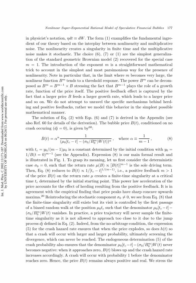
The solution of Eq. (2) with Eqs. (6) and (7) is derived in the Appendix (seealso Ref. 60 for details of the derivation). The bubble price B(t), conditioned on nocrash occuring (dj = 0), is given by60:

B(t) = αα1

(µ0[tc − t]− (σ0/Bm0 )W (t))α, where α ≡ 1

m− 1, (8)

with tc = y0/(m− 1)µ0 is a constant determined by the initial condition with y0 =1/B(t = 0)m−1 (see the Appendix). Expression (8) is our main formal result andis illustrated in Fig. 1. To grasp its meaning, let us first consider the deterministiccase σ0 = 0, such that the return rate µ(B) ∝ [B(t)]m−1 is the sole driving term.Then, Eq. (8) reduces to B(t) ∝ 1/[tc − t]1/(m−1), i.e., a positive feedback m > 1of the price B(t) on the return rate µ creates a finite-time singularity at a criticaltime tc determined by the initial starting point. This power law acceleration of theprice accounts for the effect of herding resulting from the positive feedback. It is inagreement with the empirical finding that price peaks have sharp concave upwardsmaxima.20 Reintroducing the stochastic component σ0 6= 0, we see from Eq. (8) thatthe finite-time singularity still exists but its visit is controlled by the first passageof a biased random walk at the position µ0tc such that the denominator µ0[tc− t]−(σ0/B

m0 )W (t) vanishes. In practice, a price trajectory will never sample the finite-

time singularity as it is not allowed to approach too close to it due to the jumpprocess dj defined in Eq. (2). Indeed, from the no-arbitrage condition, the expression(5) for the crash hazard rate ensures that when the price explodes, so does h(t) sothat a crash will occur with larger and larger probability, ultimately screening thedivergence, which can never be reached. The endogeneous determination (5) of thecrash probability also ensures that the denominator µ0[tc− t]−(σ0/B

m0 )W (t) never

becomes negative: when it approaches zero,B(t) blows up and the crash hazard rateincreases accordingly. A crash will occur with probability 1 before the denominatorreaches zero. Hence, the price B(t) remains always positive and real. We stress the

Int.

J. M

od. P

hys.

C 2

002.

13:1

71-1

87. D

ownl

oade

d fr

om w

ww

.wor

ldsc

ient

ific

.com

by U

NIV

ER

SIT

Y O

F M

ICH

IGA

N o

n 06

/24/

13. F

or p

erso

nal u

se o

nly.

March 12, 2002 14:38 WSPC/141-IJMPC 00308

178 D. Sornette & J. V. Andersen

0 500 1000 1500 2000 25000

2

4B

(t)

0 500 1000 1500 2000 2500

0

0.5

1

W(t

)

0 500 1000 1500 2000 2500−0.2

0

0.2

dB(t

)

0 500 1000 1500 2000 2500−0.1

0

0.1

t

dW(t

)

Fig. 1. Typical realization of a bubble (top panel) for the parameters m = 3, y0 = 1, σ0 =√0.0003, δt = 3 · 10−3 (such that one time step corresponds typically to one day of trading on

the Nasdaq composite index, calibrated by comparing the daily volatilities), tc = 1 and B0 = 1.The underlying random walk W (t) (second panel), the bubble daily increments dB (third panel)and random walk increments dW (bottom panel) are also shown. Notice the intermittent burstsof strong volatility in the bubble compared to the featureless constant level of fluctuations of therandom walk. A numerical simulation of this process requires a discretization of the time in stepson size δt. Then, knowing the value of the randow walk W (t− δt) and the bubble price B(t− δt)at the previous time t − δt, we construct W (t) by adding an increment taken from the centeredGaussian distribution with variance δt. From this, we construct B(t) using Eq. (8). We then readoff from Eq. (5) what is the probability h(t)δt for a crash to occur during the next time step.We compare this probability to a random number ran uniformly drawn in the interval [0, 1] and

trigger a crash if ran ≤ h(t)δt. In this case, the price B(t) is changed into B(t)(1 − κ), where κis drawn from a pre-chosen distribution. In the simulations presented below, the drop κ is fixedat 20%. It is straightforward to generalize to an arbitrary distribution of jumps. After the crash,the dynamics proceeds incrementally as before, starting from this new value. If ran > h(t)δt, nocrash occurs and the dynamics can be iterated another time step. In the time series shown here,there are no crashes, except for the end point. We show just one bubble that finally crashes at theend. The highly nonlinear formula (8) transforms a featureless random walk (second and fourthpanels) into a structured time series with intermittent volatility bursts (first and third panels).

remarkably simple and elegant constraint on the dynamics provided by the rationalexpectation condition that ensures the existence and stationarity of the dynamicsat all times, notwithstanding the locally nonlinear stochastic explosive dynamics.When µ0 > 0, the random walk has a positive drift attracting the denominator inEq. (8) to zero (i.e., attracting the bubble to infinity). However, by the mechanism

Int.

J. M

od. P

hys.

C 2

002.

13:1

71-1

87. D

ownl

oade

d fr

om w

ww

.wor

ldsc

ient

ific

.com

by U

NIV

ER

SIT

Y O

F M

ICH

IGA

N o

n 06

/24/

13. F

or p

erso

nal u

se o

nly.

March 12, 2002 14:38 WSPC/141-IJMPC 00308

Nonlinear Super-Exponential Rational Model of Speculative Financial Bubbles 179

explained above, as B(t) increases, so does the crash hazard rate by the relation(5). Eventually, a crash occurs that reset the bubble to a lower price. The randomwalk with drift goes on, eventually B(t) increases again and reaches “dangerouswaters”, a crash occurs again, and so on. Note that a crash is not a certain event:an inflated bubble price can also deflate spontaneously by the random realizationof the random walk W (t), which brings back the denominator far from zero.

4. Properties of the Positive Feedback Model withMultiplicative Noise

From a mathematical point of view, the process (2) with (5, 6, 7) exists only for afinite time, whose duration is a random variable: as can be seen from the solution(8), the denominator D ≡ µ0[tc − t] − (σ0/B

m0 )W (t) is positive at the initial time

t = 0 (with W (t = 0) = 0) and drifts towards zero with average velocity µ0

decorated by the random walk W (t). It is well-known that the denominator D goesto zero with probability 1 and the probability that D remains strictly positive up totime t decays exponentially fast as t increases, with an algebraic power law prefactor1/t3/2 characteristic of the distribution of first returns to the origin of a randomwalk. The leading exponential decay is itself due to the nonzero drift µ0 and woulddisappear in the absence of bias. Thus, the process (2) with (5, 6, 7) exists overfinite lifetimes, which are exponentially distributed. The explicit analytical solution(8) shows that it is unique. From a finance mathematical point of view, we stressthat this model is free of arbitrage, a property resulting from the introduction of thecrash-jump process with hazard rate h(t) defined by Eq. (5). However, it is clearthat the market is “incomplete” in the technical sense of option/derivative theoryin Finance, as it is not possible to replicate in continuous time an arbitrary option48

by a portfolio made of the stock obeying the process (2) and of a risk-free asset.This is due to the existence of the jump/crash process: this feature is well-knownfor jump processes.48

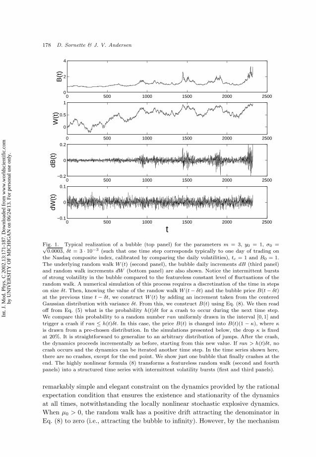
In agreement with empirical observations, returns ln[B(t + τ)/B(t)] are un-correlated by definition of the RE dynamics (2) with (5). The absolute values ofthe returns exhibit long-range correlations in good agreement with empirical data.Figure 2 shows, as a function of time-lag, the correlation function of the absolutevalues of the returns constructed from the process (9) taking into account that theobserved price is the sum of a fundamental price F and of the bubble component.The correlation function decays extremely slowly as a function of time-lag with adecay approximately linear in the logarithm of time (which is also compatible witha power law decay with a small exponent).19 This behavior is associated with clus-tering of volatility driven by the nonlinear hyperbolic structure of the dynamics (8).This result is obtained by averaging over many bubbles. Conditioned on a singlebubble and provided no crash has yet occurred, the correlation function can actuallybe nonstationary and grow with time as the bubble approaches stochastically thecritical time tc. This prediction of our model is actually born out by measurements

Int.

J. M

od. P

hys.

C 2

002.

13:1

71-1

87. D

ownl

oade

d fr

om w

ww

.wor

ldsc

ient

ific

.com

by U

NIV

ER

SIT

Y O

F M

ICH

IGA

N o

n 06

/24/

13. F

or p

erso

nal u

se o

nly.

March 12, 2002 14:38 WSPC/141-IJMPC 00308

180 D. Sornette & J. V. Andersen

100

101

102

−0.02

0

0.02

0.04

0.06

0.08

0.1

0.12

0.14

time t

F = 0.3 (o), 0.5 (*), 1 (x), 2 (.), 4 (+), and 8 (square)

Tw

o po

int c

orre

latio

n fu

nctio

n of

abs

olut

e re

turn

s

Fig. 2. Two point correlation function of the absolute value of the return of the price P (t)defined by Eq. (9) as a function of time lag in logarithmic scale (one time step correspondsapproximately to one trading day). The correlation function is calculated as a statistical averageover 300 independent bubbles B(t), where each bubble was run for 1000 time steps. Differentpoints correspond to different values of the fundamental price F . The parameters of the bubblesB(t) are m = 3, V = 0.0003, µ0 = 0.01, κ = 0.2, σ0 =

√0.0003 and B0 = 1.0. The interest rate r

is 4% annualized.

of price dynamics prior to the major crashes, which will be reported in full detailselsewhere.60

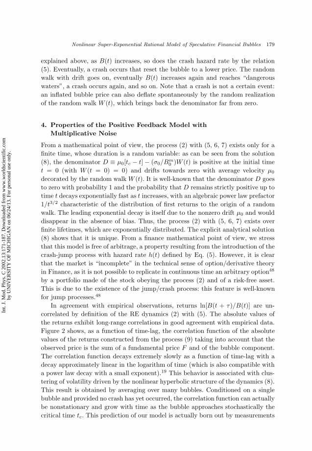
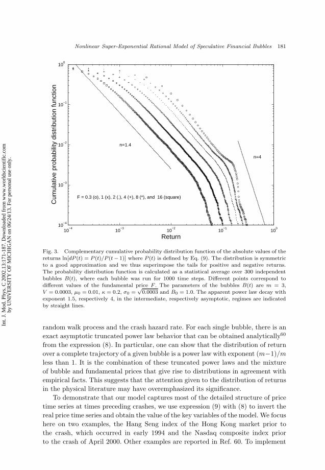
Figure 3 shows that the empirical distribution of returns is also recovered with noadjustment of parameters. To construct a meaningful distribution, we have addeda constant fundamental price F to the bubble price B(t) as only their sum isobservable in real life:

P (t) = ert[F +B(t)] . (9)

We can also include the possibility for a interest rate r or growth of the economywith rate r. Different curves for various values of F demonstrate the remarkable ro-bustness of the distributions with respect to the choice of the unknown fundamentalvalue. We observe an approximate power law decay with exponent close to 1.5 inan intermediate regime, followed by a faster decay with exponent approximately 4,in agreement with previously reported values.17,62 These apparent power law resultfrom the superposition of the contribution of many bubbles approaching towardstheir finite-time singularity within varying distances constrained by the underlying

Int.

J. M

od. P

hys.

C 2

002.

13:1

71-1

87. D

ownl

oade

d fr

om w

ww

.wor

ldsc

ient

ific

.com

by U

NIV

ER

SIT

Y O

F M

ICH

IGA

N o

n 06

/24/

13. F

or p

erso

nal u

se o

nly.

March 12, 2002 14:38 WSPC/141-IJMPC 00308

Nonlinear Super-Exponential Rational Model of Speculative Financial Bubbles 181

10−4

10−3

10−2

10−1

100

10−4

10−3

10−2

10−1

100

Return

F = 0.3 (o), 1 (x), 2 (.), 4 (+), 8 (*), and 16 (square)

Cum

ulat

ive

prob

abili

ty d

istr

ibut

ion

func

tion

n=1.4

n=4

Fig. 3. Complementary cumulative probability distribution function of the absolute values of thereturns ln[dP (t) = P (t)/P (t− 1)] where P (t) is defined by Eq. (9). The distribution is symmetricto a good approximation and we thus superimpose the tails for positive and negative returns.The probability distribution function is calculated as a statistical average over 300 independentbubbles B(t), where each bubble was run for 1000 time steps. Different points correspond todifferent values of the fundamental price F . The parameters of the bubbles B(t) are m = 3,V = 0.0003, µ0 = 0.01, κ = 0.2, σ0 =

√0.0003 and B0 = 1.0. The apparent power law decay with

exponent 1.5, respectively 4, in the intermediate, respectively asymptotic, regimes are indicatedby straight lines.

random walk process and the crash hazard rate. For each single bubble, there is anexact asymptotic truncated power law behavior that can be obtained analytically60

from the expression (8). In particular, one can show that the distribution of returnover a complete trajectory of a given bubble is a power law with exponent (m−1)/mless than 1. It is the combination of these truncated power laws and the mixtureof bubble and fundamental prices that give rise to distributions in agreement withempirical facts. This suggests that the attention given to the distribution of returnsin the physical literature may have overemphasized its significance.

To demonstrate that our model captures most of the detailed structure of pricetime series at times preceding crashes, we use expression (9) with (8) to invert thereal price time series and obtain the value of the key variables of the model. We focushere on two examples, the Hang Seng index of the Hong Kong market prior tothe crash, which occurred in early 1994 and the Nasdaq composite index priorto the crash of April 2000. Other examples are reported in Ref. 60. To implement

Int.

J. M

od. P

hys.

C 2

002.

13:1

71-1

87. D

ownl

oade

d fr

om w

ww

.wor

ldsc

ient

ific

.com

by U

NIV

ER

SIT

Y O

F M

ICH

IGA

N o

n 06

/24/

13. F

or p

erso

nal u

se o

nly.

March 12, 2002 14:38 WSPC/141-IJMPC 00308

182 D. Sornette & J. V. Andersen

the inversion of Eq. (9) with Eq. (8), we note that if these equations represent themarket behavior faithfully, then starting from a real price time series P (t), the timesseries

W (t) ≡ [P (t)e−rt − F ]−(m−1) (10)

should be a bias random walk, characterized by a constant drift M = µ0/α andvolatility

√V = σ0/αB

m0 . In other words, the inversion (10) should whiten and

Gaussianize the empirical price series. This inversion has the important advantageof not requiring the determination of the critical time tc, which appears as a constantterm in W (t).

−2 −1 0 1 2

x 10−3

0.2

0.4

0.6

0.8

1HSI: best model fit of dW to a Gaussian

dW

Cum

ulat

ive

prob

abili

ty

−300 −200 −100 0 100 200 300

0.2

0.4

0.6

0.8

1HSI: best direct fit of dP to a Gaussian

dP

Cum

ulat

ive

prob

abili

ty

−2 −1 0 1 2

x 10−3

0.2

0.4

0.6

0.8

1

dW

Cum

ulat

ive

prob

abili

ty

NAS: best model fit of dW to a Gaussian

−300 −200 −100 0 100 200 300

0.2

0.4

0.6

0.8

1

dP

Cum

ulat

ive

prob

abili

ty

NAS: best direct fit of dP to a Gaussian

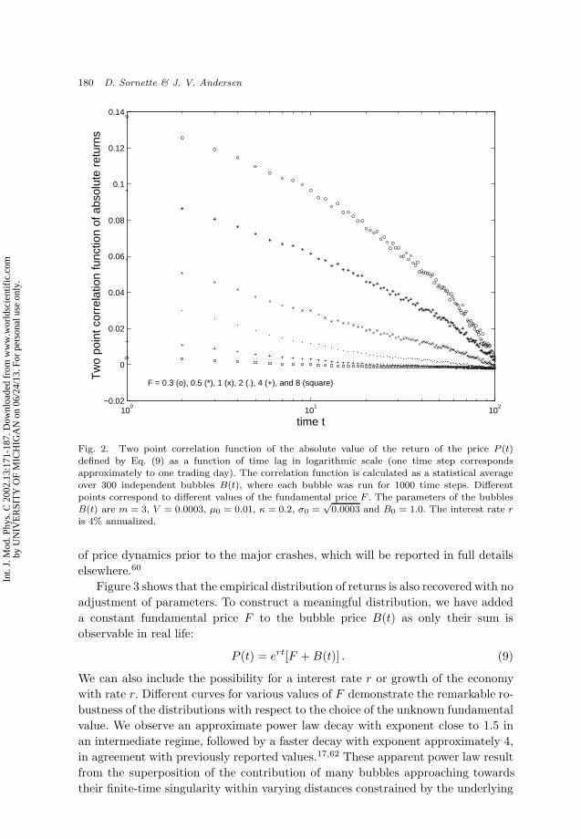
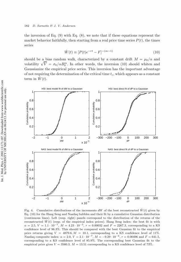
Fig. 4. Cumulative distributions of the increments dW of the best reconstructed W (t) given byEq. (10) for the Hang Seng and Nasdaq bubbles and their fit by a cumulative Gaussian distribution(continuous lines). Left (resp. right) panels correspond to the distribution of the returns of thereconstructed W (t) (resp. of the empirical index prices). Hang Seng index: the best fit is withα = 2.5, V = 1.1 · 10−7, M = 4.23 · 10−5, r = 0.00032 and F = 2267.3, corresponding to a KSconfidence level of 96.3%. This should be compared with the best Gaussian fit to the empiricalprice returns giving V = 4879.6,M = 10.1, corresponding to a KS confidence level of 11%.Nasdaq composite index: α = 2.0, V = 2.1 · 10−7, M = −9.29 · 10−6, r = 0.00496 and F = 641.5,corresponding to a KS confidence level of 85.9%. The corresponding best Gaussian fit to theempirical price gives V = 3560.3, M = 13.51 corresponding to a KS confidence level of 73%.

Int.

J. M

od. P

hys.

C 2

002.

13:1

71-1

87. D

ownl

oade

d fr

om w

ww

.wor

ldsc

ient

ific

.com

by U

NIV

ER

SIT

Y O

F M

ICH

IGA

N o

n 06

/24/

13. F

or p

erso

nal u

se o

nly.

March 12, 2002 14:38 WSPC/141-IJMPC 00308

Nonlinear Super-Exponential Rational Model of Speculative Financial Bubbles 183

To test this hypothesis, we start from an arbitrary set of the five parameters m,V , M , r, F of the model and construct W (t) using Eq. (10). We then analyze W (t)to check whether it is indeed a pure random walk. For this, we use a battery oftests. First, we check that the correlation function of the increments dW of W (t) iszero up to the statistical noise. As a second test, we investigate the distance of thedistribution of W (t) from a Gaussian distribution. We have used the Kolmogorov–Smirnov (KS) test and Anderson–Darling test to qualify the quality of the Gaussiandescription of W (t). We use the KS distance as a cost function to minimize to getthe optimal set of parameters m, V , M , r, F . We have organized hierarchically thesearch and find60 that the two leading parameters explaining most of the data arethe exponent m and the variance V of the random walk as it should. The qualityof the inversion is weakly sensitive to M , even less to r and almost insensitive tothe fundamental value F , suggesting that observed prices at times of acceleratedbubbles are mostly determined by the bubble component. Figure 4 shows the cumu-lative distributions of the increments dW of the best reconstructed W (t) and of theempirical price variations and their fit by a cumulative Gaussian distribution, forthe Hang Seng 1994 and Nasdaq 2000 bubbles. The inversion procedure is almostperfect for the Hang Seng index and of good quality but not perfect for the Nasdaqindex. For the Hang Seng bubble, the KS confidence level that the distribution isGaussian goes from 11% to 96% when going from the empirical price to the trans-formed variable W (t) defined by Eq. (10). In other words, the whitening inversionis such that it is not possible to reject the hypothesis that W (t) is a genuine randomwalk, while the corresponding hypothesis for the empirical price is rejected. For theNasdaq bubble, the gain in statistical significance is less striking, from 73% to 86%but the visual appearance of the fits is significantly better.

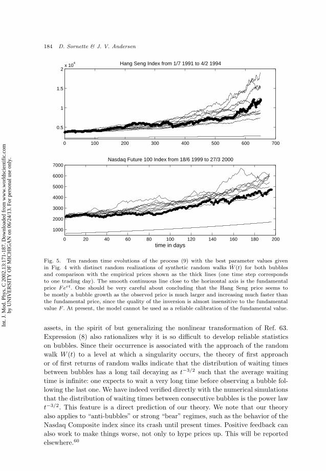
Figure 5 shows ten random time evolutions of the process (9) with the abovebest parameter values with distinct random realizations of synthetic random walksW (t) for both bubbles and compare them with the empirical prices. This figureillustrates the fact that the empirical prices can be seen as specific realizationsamong an ensemble of possible scenarios. Our model is able to capture remarkablywell the visual acceleration of these indices as a function of time. We stress thatstandard models of exponential growth would not give such a good fit.

Our nonlinear model with positive feedback together with the inversion pro-cedure (10) provides a new direct tool for detecting bubbles, for identifying theirstarting times and the plausible ends. Changing the initial time of the time series,the KS probability of the resulting Gaussian fit of the transformed series W (t) al-lows us to determine the starting date beyond which the model becomes inadequateat a given statistical level. Furthermore, the exponent m (or equivalently α) pro-vides a direct measure of the speculative mood. m = 1 is the normal regime, whilem > 1 quantifies a positive self-reinforcing feedback. This opens the possibility tocontinuously monitor it via the inversion formula (10) and use it as a “thermome-ter” of speculation, as will be reported elsewhere.60 Furthermore, the variance V ofthe multiplicative noise is a robust measure of volatility. Its continuous monitoringvia the inversion formula (10) suggests new ways at looking at dependence between

Int.

J. M

od. P

hys.

C 2

002.

13:1

71-1

87. D

ownl

oade

d fr

om w

ww

.wor

ldsc

ient

ific

.com

by U

NIV

ER

SIT

Y O

F M

ICH

IGA

N o

n 06

/24/

13. F

or p

erso

nal u

se o

nly.

March 12, 2002 14:38 WSPC/141-IJMPC 00308

184 D. Sornette & J. V. Andersen

0 100 200 300 400 500 600 700

0.5

1

1.5

2x 10

4 Hang Seng Index from 1/7 1991 to 4/2 1994

0 20 40 60 80 100 120 140 160 180 200

1000

2000

3000

4000

5000

6000

7000

time in days

Nasdaq Future 100 Index from 18/6 1999 to 27/3 2000

Fig. 5. Ten random time evolutions of the process (9) with the best parameter values givenin Fig. 4 with distinct random realizations of synthetic random walks W (t) for both bubblesand comparison with the empirical prices shown as the thick lines (one time step correspondsto one trading day). The smooth continuous line close to the horizontal axis is the fundamentalprice Fert. One should be very careful about concluding that the Hang Seng price seems tobe mostly a bubble growth as the observed price is much larger and increasing much faster thanthe fundamental price, since the quality of the inversion is almost insensitive to the fundamentalvalue F . At present, the model cannot be used as a reliable calibration of the fundamental value.

assets, in the spirit of but generalizing the nonlinear transformation of Ref. 63.Expression (8) also rationalizes why it is so difficult to develop reliable statisticson bubbles. Since their occurrence is associated with the approach of the randomwalk W (t) to a level at which a singularity occurs, the theory of first approachor of first returns of random walks indicate that the distribution of waiting timesbetween bubbles has a long tail decaying as t−3/2 such that the average waitingtime is infinite: one expects to wait a very long time before observing a bubble fol-lowing the last one. We have indeed verified directly with the numerical simulationsthat the distribution of waiting times between consecutive bubbles is the power lawt−3/2. This feature is a direct prediction of our theory. We note that our theoryalso applies to “anti-bubbles” or strong “bear” regimes, such as the behavior of theNasdaq Composite index since its crash until present times. Positive feedback canalso work to make things worse, not only to hype prices up. This will be reportedelsewhere.60

Int.

J. M

od. P

hys.

C 2

002.

13:1

71-1

87. D

ownl

oade

d fr

om w

ww

.wor

ldsc

ient

ific

.com

by U

NIV

ER

SIT

Y O

F M

ICH

IGA

N o

n 06

/24/

13. F

or p

erso

nal u

se o

nly.

March 12, 2002 14:38 WSPC/141-IJMPC 00308

Nonlinear Super-Exponential Rational Model of Speculative Financial Bubbles 185

5. Conclusion

In summary, we have presented a nonlinear model with positive feedback and mul-tiplicative noise, which explains in a parsimonious and economically intuitive wayessentially all the characteristics of empirical financial time series, including thespontaneous emergence of speculative bubbles. It could provide a simple startingpoint for multivariate modeling of financial and economic variables. We shall reportelsewhere the results of our tests using this model to identify periods of nonlinearbubbles from periods of “normal” times and how our model allows us to distinguishthese two regimes quantitatively.

Acknowledgments

We thank T. Lux for discussions. J. V. Andersen acknowledges support from CNRS,France. D. Sornette gratefully acknowledges support from the James S. McDonnellFoundation 21st Century Scientist award/studying complex systems.

Appendix. Derivation of the Bubble Solution

In this Appendix, we derive the solution (8). Changing variable from B to y =φ(B) = 1/Bm−1, Ito calculus tells us that the coefficients µ(B)B and σ(B)B of anequation of the form dB = µ(B)Bdt+ σ(B)BdW are changed into:

µ(y) = µ(B)Bdφ

dB+

12

[σ(B)B]2d2φ

dB2

= −µ(B)Bm− 1Bm

+12

[σ(B)B]2m(m− 1)Bm+1

, (A.1)

σ(y) = σ(B)Bdφ

dB= −σ(B)B

m− 1Bm

, (A.2)

where dy = µ(y)dt+ σ(y)dW .With the parameterization (6), (7), the equation on y becomes:

dy = −(m− 1)µ0 dt−1

Bm−11

dW , (A.3)

where

B1 =(

Bm0(m− 1)σ0

)1/(m−1)

. (A.4)

By the nonlinear change of variable y = 1/Bm−1, we thus recover a simple Brownianmotion with constant drift and constant volatility in the variable y. The solutionof Eq. (A.3) is:

y(t) = y0 − (m− 1)µ0t−1

Bm−11

W (t) . (A.5)

y0 is the initial value y(0) = y0 = 1/B(t = 0)m−1.

Int.

J. M

od. P

hys.

C 2

002.

13:1

71-1

87. D

ownl

oade

d fr

om w

ww

.wor

ldsc

ient

ific

.com

by U

NIV

ER

SIT

Y O

F M

ICH

IGA

N o

n 06

/24/

13. F

or p

erso

nal u

se o

nly.

March 12, 2002 14:38 WSPC/141-IJMPC 00308

186 D. Sornette & J. V. Andersen

In terms of the price B(t), we get Eq. (8) by inverting y = 1/Bm−1 wheretc = y0/(m−1)µ0 is a constant determined by the initial condition. It is importantto stress that a finite-time singularity occurs when the denominator of the right-hand-side of Eq. (8) goes to zero. In absence of noise (σ0 = 0), tc is the criticaltime. However, in the general case with σ0 > 0, the finite-time singularity occursat a random time no more equal to tc, which depends on the specific realization ofthe random walk W (t).

References

1. P. W. Anderson, K. J. Arrow, and D. Pines (eds.), The Economy as an EvolvingComplex System (Addison-Wesley, New York, 1988).

2. D. Sornette, “Predictability of catastrophic events: Material rupture, earthquakes,turbulence, financial crashes and human birth,” Proc. Nat. Acad. Sci. USA, in press(2001); http://arXiv.org/abs/cond-mat/0107173.

3. D. Sornette, F. Ferre, and E. Papiernik, Int. J. Bifurcation and Chaos 4, 693 (1994).4. S. C. Jaume and L. R. Sykes, Pure Appl. Geophys. 155, 279 (1999).5. S. G. Sammis and D. Sornette, Proc. Nat. Acad. Sci. USA, in press (2001);

http://arXiv.org/abs/cond-mat/0107143.6. W. B. Arthur, Center for Economic Policy Res. 111, 1 (1987).7. A. Johansen, D. Sornette, and O. Ledoit, J. Risk 1, 5 (1999).8. R. B. Pandey and D. Stauffer, Int. J. Theor. Appl. Fin. 3, 479 (2000).9. K. Ide and D. Sornette, “Oscillatory finite-time singularities in finance, population

and rupture,” accepted in Physica A; http://arXiv.org/abs/cond-mat/0106047.10. D. Sornette and K. Ide, “Theory of self-similar oscillatory finite-time singularities in

finance, population and rupture,” http://arXiv.org/abs/cond-mat/0106054.11. A. Proykova, L. Russenova, and D. Stauffer, “Nucleation of market shocks in Sornette–

Ide model,” http://xxx.lanl.gov/abs/cond-mat/0110124.12. D. Sornette and A. Johansen, Quantitative Finance 1(4), 452 (2001).13. J. Y. Campbell, A. W. Lo, and A. C. MacKinlay, The Econometrics of Financial

Markets (Princeton University Press, Princeton, NJ, 1997).14. Z. Ding, C. W. J. Granger, and R. Engle, J. Empirical Finance 1, 83 (1993).15. B. B. Mandelbrot, J. Business 36, 392 (1963).16. C. G. de Vries, in The Handbook of International Macroeconomics, ed. F. van der

Ploeg (Blackwell, Oxford, 1994).17. R. N. Mantegna and H. E. Stanley, Nature 376, 46 (1995).18. B. B. Mandelbrot, Fractals and Scaling in Finance: Discontinuity, Concentration, Risk

(Springer, New York, 1997).19. J.-F. Muzy, D. Sornette, J. Delour, and A. Arneodo, Quantitative Finance 1, 131

(2001).20. B. M. Roehner and D. Sornette, Eur. Phys. J. B 4, 387 (1998).21. B. LeBaron, W. B. Arthur, and R. Palmer, J. Economic Dyn. Control 23, 1487 (1999).22. J. D. Farmer, “Market force, ecology and evolution,” (1998); preprint available at

adap-org/9812005.23. B. Rachlevsky-Reich et al., Information Syst. 24, 495 (1999).24. C. H. Hommes, Quantitative Finance 1, 149 (2001).25. B. LeBaron, J. Economic Dyn. Control 24(5–7), 679 (2000).26. D. Challet and Y.-C. Zhang, Physica A 246, 407 (1997).27. A. Kirman, in Money and Financial Markets, ed. M. Taylor (Macmillan, 1991).

Int.

J. M

od. P

hys.

C 2

002.

13:1

71-1

87. D

ownl

oade

d fr

om w

ww

.wor

ldsc

ient

ific

.com

by U

NIV

ER

SIT

Y O

F M

ICH

IGA

N o

n 06

/24/

13. F

or p

erso

nal u

se o

nly.

March 12, 2002 14:38 WSPC/141-IJMPC 00308

Nonlinear Super-Exponential Rational Model of Speculative Financial Bubbles 187

28. T. Lux, Economic J. 105, 881 (1995).29. T. Lux and M. Marchesi, Nature 397, 498 (1999).30. M. Youssefmir, B. A. Huberman, and T. Hogg, Comput. Economics 12, 97 (1998).31. A. H. Sato and H. Takayasu, Physica A 250, 231 (1998).32. S. M. de Oliveira, P. M. C de Oliveira, and D. Stauffer, Evolution, Money, War and

Computers (Teubner, Stuttgart-Leipzig, 1999).33. M. Levy, H. Levy, and S. Solomon, The Microscopic Simulation of Financial Markets:

From Investor Behavior to Market Phenomena (Academic Press, San Diego, 2000).34. A. Gaunersdorfer, J. Economic Dyn. Control 24, 799 (2000).35. D. Gillette and R. DelMas, Newsletter published by Department of Economics,

Management and Accounting, Marietta College, Fall 1992, 1, pp. 1–5.36. V. L. Smith, J. Economic Literature 34, 1950 (1996).37. D. Davis and C. Holt, Experimental Economics (Princeton University Press, Prince-

ton, NJ, 1993).38. J. Kagel and A. Roth (eds.), Handbook of Experimental Economics (Princeton Uni-

versity Press, Princeton, NJ, 1995).39. C. R. Plott and S. Sunder, Econometrica 56, 1085 (1988).40. R. Forsythe, T. R. Palfrey, and C. R. Plott, Econometrica 50, 537 (1982).41. O. J. Blanchard, Economics Lett. 3, 387 (1979).42. O. J. Blanchard and M. W. Watson, in Crisis in Economic and Financial Structure:

Bubbles, Bursts, and Shocks, ed. P. Wachtel (Lexington Books, Lexington, 1982).43. C. Camerer, J. Economic Surveys 3, 3 (1989).44. M. C. Adam and A. Szafarz, Oxford Economic Papers 44, 626 (1992).45. G. W. Evans, American Economic Rev. 81, 922 (1991).46. W. T. Woo, J. Money, Credit and Banking 19, 499 (1987).47. T. Lux and D. Sornette, “On rational bubbles and fat tails,” in press in the J. Money,

Credit and Banking; e-print at cond-mat/9910141.48. R. C. Merton, Continuous-Time Finance (Blackwell, Cambridge, 1990).49. J. C. Cox, S. A. Ross, and M. Rubinstein, J. Financial Economics 7, 229 (1979).50. R. C. Merton, J. Financial Economics 3, 125 (1976).51. A. Johansen, O. Ledoit, and D. Sornette, Int. J. Theor. Appl. Fin. 3, 219 (2000).52. G.-R. Kim and H. M. Markowitz, J. Portfolio Management 16, 45 (1989).53. R. J. Shiller, Irrational Exuberance (Princeton University Press, Princeton, NJ, 2000).54. D. S. Scharfstein and J. C. Stein, American Economic Rev. 80, 465 (1990).55. M. Grinblatt, S. Titman, and R. Wermers, American Economic Rev. 85, 1088 (1995).56. B. Trueman, Rev. Financial Studies 7, 97 (1991).57. S. Bikhchandani, D. Hirshleifer, and I. Welch, J. Economic Perspectives 12, 151

(1998).58. D. A. Hsieh, Financial Analysts J. 55 (1995).59. R. Sircar and G. Papanicolaou, Appl. Math. Finance 5, 45 (1998).60. J. Andersen and D. Sornette, “Rational models of nonlinear bubbles and crashes,”

working paper (2001).61. D. Sornette, Critical Phenomena in Natural Sciences, Springer Series in Synergetics

(Springer, Heidelberg, 2000).62. P. Gopikrishnan, M. Meyer, L. A. N. Amaral, and H. E. Stanley, Eur. Phys. J. B 3,

139 (1998).63. D. Sornette, P. Simonetti, and J. V. Andersen, Phys. Rep. 335, 19 (2000).

Int.

J. M

od. P

hys.

C 2

002.

13:1

71-1

87. D

ownl

oade

d fr

om w

ww

.wor

ldsc

ient

ific

.com

by U

NIV

ER

SIT

Y O

F M

ICH

IGA

N o

n 06

/24/

13. F

or p

erso

nal u

se o

nly.

This article has been cited by:

1. L. Lin, D. Sornette. 2013. Diagnostics of rational expectation financial bubbles with stochasticmean-reverting termination times. The European Journal of Finance 19:5, 344-365. [CrossRef]

2. Young-Mee Kwon, In-Tae Jeon, Hye-Jeong Kang. 2010. ENDOGENOUS DOWNWARDJUMP DIFFUSION AND BLOW UP PHENOMENA BEFORE CRASH. Bulletin of theKorean Mathematical Society 47:6, 1105-1119. [CrossRef]

3. Wanfeng Yan, Ryan Woodard, Didier Sornette. 2010. Diagnosis and prediction of tipping pointsin financial markets: Crashes and rebounds. Physics Procedia 3:5, 1641-1657. [CrossRef]

4. Taisei Kaizoji, Didier SornetteBubbles and Crashes . [CrossRef]5. Kota Watanabe, Hideki Takayasu, Misako Takayasu. 2009. Random walker in temporally

deforming higher-order potential forces observed in a financial crisis. Physical Review E 80:5. .[CrossRef]

6. V.I. Yukalov, D. Sornette, E.P. Yukalova. 2009. Nonlinear dynamical model of regime switchingbetween conventions and business cycles. Journal of Economic Behavior & Organization 70:1-2,206-230. [CrossRef]

7. D. Sornette. 2008. Nurturing breakthroughs: lessons from complexity theory. Journal ofEconomic Interaction and Coordination 3:2, 165-181. [CrossRef]

8. Weigang Wan, Giovanni Lapenta. 2008. Electron Self-Reinforcing Process of MagneticReconnection. Physical Review Letters 101:1. . [CrossRef]

9. Kota Watanabe, Hideki Takayasu, Misako Takayasu. 2007. A mathematical definition of thefinancial bubbles and crashes. Physica A: Statistical Mechanics and its Applications 383:1, 120-124.[CrossRef]

10. Kota Watanabe, Hideki Takayasu, Misako Takayasu. 2007. Extracting the exponential behaviorsin the market data. Physica A: Statistical Mechanics and its Applications 382:1, 336-339.[CrossRef]

11. A. KRAWIECKI. 2005. MICROSCOPIC SPIN MODEL FOR THE STOCK MARKETWITH ATTRACTOR BUBBLING AND HETEROGENEOUS AGENTS. InternationalJournal of Modern Physics C 16:04, 549-559. [Abstract] [References] [PDF] [PDF Plus]

12. Gerrit Broekstra, Didier Sornette, Wei-Xing Zhou. 2005. Bubble, critical zone and the crash ofRoyal Ahold. Physica A: Statistical Mechanics and its Applications 346:3-4, 529-560. [CrossRef]

13. Wei-Xing Zhou, Didier Sornette. 2003. Evidence of a worldwide stock market log-periodic anti-bubble since mid-2000. Physica A: Statistical Mechanics and its Applications 330:3-4, 543-583.[CrossRef]

14. Hans Fogedby. 2003. Damped finite-time singularity driven by noise. Physical Review E 68:5. .[CrossRef]

15. Wei-Xing Zhou, Didier Sornette. 2003. 2000–2003 real estate bubble in the UK but not in theUSA. Physica A: Statistical Mechanics and its Applications 329:1-2, 249-263. [CrossRef]

16. WEI-XING ZHOU, DIDIER SORNETTE. 2003. NONPARAMETRIC ANALYSES OFLOG-PERIODIC PRECURSORS TO FINANCIAL CRASHES. International Journal ofModern Physics C 14:08, 1107-1125. [Abstract] [References] [PDF] [PDF Plus]

17. D Sornette. 2003. Critical market crashes. Physics Reports 378:1, 1-98. [CrossRef]

Int.

J. M

od. P

hys.

C 2

002.

13:1

71-1

87. D

ownl

oade

d fr

om w

ww

.wor

ldsc

ient

ific

.com

by U

NIV

ER

SIT

Y O

F M

ICH

IGA

N o

n 06

/24/

13. F

or p

erso

nal u

se o

nly.

18. Didier Sornette, Wei-Xing Zhou. 2002. The US 2000-2002 market descent: how much longerand deeper?. Quantitative Finance 2:6, 468-481. [CrossRef]

19. Hans Fogedby, Vakhtang Poutkaradze. 2002. Power laws and stretched exponentials in a noisyfinite-time-singularity model. Physical Review E 66:2. . [CrossRef]

20. D. Sornette. 2002. “Slimming” of power-law tails by increasing market returns. Physica A:Statistical Mechanics and its Applications 309:3-4, 403-418. [CrossRef]

Int.

J. M

od. P

hys.

C 2

002.

13:1

71-1

87. D

ownl

oade

d fr

om w

ww

.wor

ldsc

ient

ific

.com

by U

NIV

ER

SIT

Y O

F M

ICH

IGA

N o

n 06

/24/

13. F

or p

erso

nal u

se o

nly.