Embed Size (px)
Citation preview
A Nonlinear Neural Network-Based Model Predictive Controlfor Industrial Gas Turbine
by
Ibrahem Mohamed Atia IBRAHEM
THESIS PRESENTED TO ÉCOLE DE TECHNOLOGIE SUPÉRIEURE
IN PARTIAL FULFILLMENT FOR THE DEGREE OF
DOCTOR OF PHILOSOPHY
Ph.D.
MONTREAL, OCTOBER 22, 2020
ÉCOLE DE TECHNOLOGIE SUPÉRIEUREUNIVERSITÉ DU QUÉBEC
Ibrahem Mohamed Atia Ibrahem, 2020

This Creative Commons license allows readers to download this work and share it with others as long as the
author is credited. The content of this work cannot be modified in any way or used commercially.

BOARD OF EXAMINERS
THIS THESIS HAS BEEN EVALUATED
BY THE FOLLOWING BOARD OF EXAMINERS
Mrs. Ouassima Akhrif, Thesis Supervisor
Department of Electrical Engineering, École de technologie supérieure
M. Hany Moustapha, Co-supervisor
Department of Mechanical Engineering, École de technologie supérieure
M. Pierre Bélanger, President of the Board of Examiners
Department of Mechanical Engineering, École de technologie supérieure
Mrs. Lyne Woodward, Member of the jury
Department of Electrical Engineering, École de technologie supérieure
M. David May, External Independent Examiner
Siemens Energy Canada Limited
M. Guchuan Zhu, External Examiner
Department of Electrical Engineering, Ecole Polytechnique de Montreal
THIS THESIS WAS PRESENTED AND DEFENDED
IN THE PRESENCE OF A BOARD OF EXAMINERS AND THE PUBLIC
ON OCTOBER 15, 2020
AT ÉCOLE DE TECHNOLOGIE SUPÉRIEURE

IV

ACKNOWLEDGEMENTS
The present document, resulting of three years of research, would not have been possible with-
out the help, encouragements and support of many persons. I thank all of them and I present
them all my gratitude.
Firstly, I would like to acknowledge my direct supervisors Professor Ouassima Akhrif and
Professor Hany Moustapha for their enthusiasm, inspiration, and huge efforts to explain things
clearly and simply. I would have never finished this thesis without their constant support,
encouragement, and stimulating advice. All of these helped me a lot in maintaining my
confidence to continue my research. I would also like to thank the project leader Mr. Mar-
tin.Staniszewski at Siemens Energy Canada Limited for helping and supporting me. He gener-
ously gave much time and effort to help me.
I would like to thank the Egyptian Ministry of defense for funding me and École de technologie
supérieure for accepting me in its graduate program and motivating me to do this work. Also,
I thank Siemens Energy Canada Limited R & D center for providing me the opportunity to use
their products to perform my simulations and helping me to fill out the gap between academia
and industry. I cannot end without thanking my engineering friends for sharing their knowledge
regarding the electric department.
Finally, My deepest thanks to who enlighten my life with happiness, my lovely wife Reham
and my son Asser for their love, patience, encouragement, and support. I am indebted to my
mother, my father, and my sisters for their support that they offered me over my studying years.
And here in, I wish my sister Ghada to be proud of me.


Commande prédictive non linéairebasée sur un réseau neuronal pour une turbine à gaz
industrielle
Ibrahem Mohamed Atia IBRAHEM
RÉSUMÉ
Les turbines à gaz sont largement utilisées actuellement dans l’aviation, les applications pétrol-
ières et gazières et la production d’électricité. Avec cette utilisation croissante dans une large
gamme d’applications, les turbines à gaz sont conçues pour fonctionner dans une large plage
de fonctionnement. Typiquement, la température ambiante peut varier considérablement d’une
chaude journée d’été à une froide nuit d’hiver. Aussi, différents types de carburant peuvent
être utilisés. De plus, les performances d’un turbomoteur se détériorent à l’usage en raison
de la dégradation des composants provoquée par l’érosion et la corrosion. Ces exigences pour
garantir des niveaux de performance élevés tout en maintenant la stabilité et un fonctionnement
sûr avec un coût global minimal imposent de grands défis à la conception du système de com-
mande. Dans cette thèse, de nouvelles approches pour la modélisation de turbines à gaz et
la conception de contrôleurs avancés multivariables sont étudiées. Une approche de contrôle
prédictif non linéaire (NMPC) basée sur un ensemble de réseaux neuronaux récurrents (NN)
est utilisée pour atteindre les objectifs de contrôle d’un moteur à turbine à gaz aérodérivé à
trois bobines Siemens SGT-A65 utilisé pour la production d’électricité. Une nouvelle méthode
d’ensemble est proposée, qui aboutit à un modèle NN adaptatif. Les résultats de la simula-
tion montrent une amélioration de la précision et de la robustesse en utilisant l’approche de
modélisation proposée. En outre, un autre gain important est le temps d’exécution très faible
(40,5 μs), qui peut permettre de nombreuses applications en temps réel qui nécessitent une
conception de contrôle basée sur un modèle.
Pour la commande en boucle fermée, un contrôleur prédictif non linéaire (NMPC) à entrées
multiples et sorties multiples (MIMO) et avec contraintes est développé sur la base de l’algori-
thme de contrôle prédictif généralisé (GPC) en raison de sa capacité à gérer les problèmes
MIMO dans un même algorithme. Dans ce contrôleur, une nouvelle approche de compromis
entre l’utilisation d’un modèle non linéaire et des approches de linéarisation successives est
utilisée afin de réduire l’effort de calcul et en même temps d’augmenter la robustesse du con-
trôleur. L’estimation des réponses libres et forcées du GPC est réalisée sur la base du modèle
NN de la turbine à chaque instant d’échantillonnage. En outre, la procédure de programmation
quadratique (QP) de Hildreth est utilisée pour résoudre le problème d’optimisation quadratique
du contrôleur NNGPC, qui offre simplicité et fiabilité dans la mise en œuvre en temps réel. Une
comparaison entre les performances du contrôleur proposé (NNGPC) et du contrôleur actuel du
moteur SGT-A65 (le contrôleur min-max) est effectuée. Les résultats de la simulation montrent
que le NNGPC donne des réponses de sortie supérieures avec moins de comportement oscilla-
toire et des actions de contrôle plus douces aux variations soudaines de la charge électrique que
celles observées pour le contrôleur min-max existant. De plus, le contrôleur NNGPC nécessite
moins d’effort de contrôle que le contrôleur min-max pour atteindre les objectifs souhaités.
La minimisation de l’effort de commande a des répercussions pratiques importantes car elle

VIII
réduit l’intensité de l’usure mécanique des actionneurs, ce qui conduit à une augmentation de
la sécurité fonctionnelle, de la durée de vie et de l’économie du processus contrôlé. De plus,
le temps de calcul nécessaire pour résoudre le problème d’optimisation était suffisamment plus
rapide que la fréquence d’échantillonnage, ce qui rend possible une implémentation en temps
réel du contrôleur NNGPC.
Mots-clés: Modèle NARX, Turbine à gaz, Modélisation, Réseaux de neurones, Ensemble,
GPC, NMPC, NNGPC.
A Nonlinear Neural Network-Based Model Predictive Control for Industrial Gas Turbine
Ibrahem Mohamed Atia IBRAHEM
ABSTRACT
Gas turbines are now extensively used in aviation, oil and gas applications and power gen-
eration. With this increasing use in a diverse range of applications, gas turbine engines are
designed to operate in a wide operating envelope. Typically, the ambient temperature can vary
substantially from a hot summer day to a cold winter night. In addition, different fuel types
may be used. Furthermore, the performance of a turbine engine deteriorates with use because
of component degradation caused by erosion and corrosion. These requirements for guaran-
teed high performance levels while maintaining stability and safe operation with minimum
overall cost impose severe challenges on control system design. In this dissertation, new ap-
proaches for gas turbine engine modelling and multivariable advanced controller design are
investigated. A nonlinear model predictive control (NMPC) approach based on an ensemble
of recurrent neural networks (NN) is utilized to achieve the control objectives for a Siemens
SGT-A65 three spool aeroderivative gas turbine engine used for power generation. A novel
ensemble method is proposed, which results in an adaptive NN model. The simulation results
show improvement in accuracy and robustness by using the proposed modelling approach.
Also, another important gain is the very rapid execution time (40,5 μs), which can support
many real time applications that require model-based control design.
For the closed-loop control, a constrained multi-input multi-output (MIMO) nonlinear model
predictive controller (NMPC) is developed based on the generalized predictive control (GPC)
algorithm because of its ability to handle MIMO problems in one algorithm. In this controller,
a novel trade-off approach between the usage of a non-linear model and successive lineariza-
tion approaches is used in order to reduce the computation effort and at the same time increase
the robustness of the controller. Estimation of the free and forced responses of the GPC are per-
formed based on the NN model of the plant at each sampling time. In addition, the Hildreth’s
Quadratic Programming (QP) procedure is utilized to solve the quadratic optimization problem
of the NNGPC controller, which offers simplicity and reliability in real-time implementation.
A comparison between the performance of the proposed controller (NNGPC) and the current
controller of the SGT-A65 engine (min-max controller) is performed. The simulation results
show that the NNGPC has demonstrated superior output responses with less oscillatory behav-
ior and smoother control actions to sudden variations in the electric load than those observed
in the existing min-max controller. Furthermore, the NNGPC controller requires less con-
trol effort than the min-max controller to achieve the desired objectives. The minimization
of control effort has significant practical repercussions because it reduces the intensity of me-
chanical wear of the actuators, which leads to an increase in the functional safety, lifetime, and
economics of the controlled process. In addition, the computation time required to solve an op-
timization problem was sufficiently shorter than the sampling period which makes a real-time
implementation of the NNGPC controller possible.

X
Keywords: NARX model, Gas turbine, Modelling, Neural Networks, Ensemble, GPC, NMPC,
NNGPC.
TABLE OF CONTENTS
Page
INTRODUCTION . . . . . . . . . . . . . . . . . . . . . . . . . . . . . . . . . . . . . . . . . . . . . . . . . . . . . . . . . . . . . . . . . . . . . . . . . . . . . . . . 1
CHAPTER 1 GAS TURBINE - OVERVIEW .. . . . . . . . . . . . . . . . . . . . . . . . . . . . . . . . . . . . . . . . . . . . 13
1.1 Introduction . . . . . . . . . . . . . . . . . . . . . . . . . . . . . . . . . . . . . . . . . . . . . . . . . . . . . . . . . . . . . . . . . . . . . . . . . . . . . . 13
1.2 Gas turbine principle of operation . . . . . . . . . . . . . . . . . . . . . . . . . . . . . . . . . . . . . . . . . . . . . . . . . . . . . . 13
1.3 Aero-derivative gas turbine engine . . . . . . . . . . . . . . . . . . . . . . . . . . . . . . . . . . . . . . . . . . . . . . . . . . . . . 16
1.3.1 Siemens SGT-A65 ADGTE - Overview . . . . . . . . . . . . . . . . . . . . . . . . . . . . . . . . . . . . . 20
1.3.1.1 Engine configuration . . . . . . . . . . . . . . . . . . . . . . . . . . . . . . . . . . . . . . . . . . . . . . 20
1.3.1.2 Engine control system . . . . . . . . . . . . . . . . . . . . . . . . . . . . . . . . . . . . . . . . . . . . 23
1.3.2 SGT-A65 ADGTE mathematical model . . . . . . . . . . . . . . . . . . . . . . . . . . . . . . . . . . . . . 26
1.3.2.1 Inlet . . . . . . . . . . . . . . . . . . . . . . . . . . . . . . . . . . . . . . . . . . . . . . . . . . . . . . . . . . . . . . . . 26
1.3.2.2 Compressor . . . . . . . . . . . . . . . . . . . . . . . . . . . . . . . . . . . . . . . . . . . . . . . . . . . . . . . . 27
1.3.2.3 Combustor . . . . . . . . . . . . . . . . . . . . . . . . . . . . . . . . . . . . . . . . . . . . . . . . . . . . . . . . . 30
1.3.2.4 Gas generator turbine . . . . . . . . . . . . . . . . . . . . . . . . . . . . . . . . . . . . . . . . . . . . . 30
1.3.2.5 Power turbine . . . . . . . . . . . . . . . . . . . . . . . . . . . . . . . . . . . . . . . . . . . . . . . . . . . . . . 31
1.3.2.6 Exhaust nozzle . . . . . . . . . . . . . . . . . . . . . . . . . . . . . . . . . . . . . . . . . . . . . . . . . . . . 31
1.3.2.7 Load . . . . . . . . . . . . . . . . . . . . . . . . . . . . . . . . . . . . . . . . . . . . . . . . . . . . . . . . . . . . . . . 32
1.3.2.8 Engine dynamics . . . . . . . . . . . . . . . . . . . . . . . . . . . . . . . . . . . . . . . . . . . . . . . . . . 32
1.4 Summary . . . . . . . . . . . . . . . . . . . . . . . . . . . . . . . . . . . . . . . . . . . . . . . . . . . . . . . . . . . . . . . . . . . . . . . . . . . . . . . . 35
CHAPTER 2 LITERATURE REVIEW .. . . . . . . . . . . . . . . . . . . . . . . . . . . . . . . . . . . . . . . . . . . . . . . . . . . 37
2.1 Introduction . . . . . . . . . . . . . . . . . . . . . . . . . . . . . . . . . . . . . . . . . . . . . . . . . . . . . . . . . . . . . . . . . . . . . . . . . . . . . . 37
2.2 Modelling and simulation of gas turbine engines . . . . . . . . . . . . . . . . . . . . . . . . . . . . . . . . . . . . . . 37
2.2.1 Physics based modelling of GTEs . . . . . . . . . . . . . . . . . . . . . . . . . . . . . . . . . . . . . . . . . . . 38
2.2.2 Data driven based modelling of GTEs . . . . . . . . . . . . . . . . . . . . . . . . . . . . . . . . . . . . . . . 44
2.3 Advanced control of gas turbine engine . . . . . . . . . . . . . . . . . . . . . . . . . . . . . . . . . . . . . . . . . . . . . . . . 48
2.4 Conclusion of literature . . . . . . . . . . . . . . . . . . . . . . . . . . . . . . . . . . . . . . . . . . . . . . . . . . . . . . . . . . . . . . . . . 54
CHAPTER 3 NEURAL NETWORKS MODELLING APPROACH . . . . . . . . . . . . . . . . . . . . . 61
3.1 Introduction . . . . . . . . . . . . . . . . . . . . . . . . . . . . . . . . . . . . . . . . . . . . . . . . . . . . . . . . . . . . . . . . . . . . . . . . . . . . . . 61
3.2 Neural network basics . . . . . . . . . . . . . . . . . . . . . . . . . . . . . . . . . . . . . . . . . . . . . . . . . . . . . . . . . . . . . . . . . . 61
3.3 ANN modelling approach . . . . . . . . . . . . . . . . . . . . . . . . . . . . . . . . . . . . . . . . . . . . . . . . . . . . . . . . . . . . . . 61
3.3.1 Data acquisition and preprocessing . . . . . . . . . . . . . . . . . . . . . . . . . . . . . . . . . . . . . . . . . . 62
3.3.2 System order and delay estimation . . . . . . . . . . . . . . . . . . . . . . . . . . . . . . . . . . . . . . . . . . . 65
3.3.3 NARX model configuration . . . . . . . . . . . . . . . . . . . . . . . . . . . . . . . . . . . . . . . . . . . . . . . . . . 67
3.3.4 The best model selection process . . . . . . . . . . . . . . . . . . . . . . . . . . . . . . . . . . . . . . . . . . . . 71
3.3.4.1 MISO-NARX model of NH . . . . . . . . . . . . . . . . . . . . . . . . . . . . . . . . . . . . . . . 73
3.3.4.2 MISO-NARX model of NI . . . . . . . . . . . . . . . . . . . . . . . . . . . . . . . . . . . . . . . 74
3.3.4.3 MISO-NARX model of NL . . . . . . . . . . . . . . . . . . . . . . . . . . . . . . . . . . . . . . . 75
3.3.4.4 MISO-NARX model of PW . . . . . . . . . . . . . . . . . . . . . . . . . . . . . . . . . . . . . . 76
XII
3.3.4.5 MISO-NARX model of T GT . . . . . . . . . . . . . . . . . . . . . . . . . . . . . . . . . . . . 77
3.3.4.6 MISO-NARX model of T30 . . . . . . . . . . . . . . . . . . . . . . . . . . . . . . . . . . . . . . . 78
3.3.4.7 MISO-NARX model of P30 . . . . . . . . . . . . . . . . . . . . . . . . . . . . . . . . . . . . . . . 80
3.3.5 Ensemble generation . . . . . . . . . . . . . . . . . . . . . . . . . . . . . . . . . . . . . . . . . . . . . . . . . . . . . . . . . . 81
3.3.6 Ensemble integration . . . . . . . . . . . . . . . . . . . . . . . . . . . . . . . . . . . . . . . . . . . . . . . . . . . . . . . . . 86
3.4 Comparison between single MISO-NARX model and ensemble of MISO-
NARX models . . . . . . . . . . . . . . . . . . . . . . . . . . . . . . . . . . . . . . . . . . . . . . . . . . . . . . . . . . . . . . . . . . . . . . . . . . . 93
3.4.1 Ensemble model of PW . . . . . . . . . . . . . . . . . . . . . . . . . . . . . . . . . . . . . . . . . . . . . . . . . . . . . . . 93
3.4.2 Ensemble model of NH . . . . . . . . . . . . . . . . . . . . . . . . . . . . . . . . . . . . . . . . . . . . . . . . . . . . . . . 95
3.4.3 Ensemble model of NI . . . . . . . . . . . . . . . . . . . . . . . . . . . . . . . . . . . . . . . . . . . . . . . . . . . . . . . . 97
3.4.4 Ensemble model of NL . . . . . . . . . . . . . . . . . . . . . . . . . . . . . . . . . . . . . . . . . . . . . . . . . . . . . . . . 99
3.4.5 Ensemble model of T GT . . . . . . . . . . . . . . . . . . . . . . . . . . . . . . . . . . . . . . . . . . . . . . . . . . . .101
3.4.6 Ensemble model of T30 . . . . . . . . . . . . . . . . . . . . . . . . . . . . . . . . . . . . . . . . . . . . . . . . . . . . . .103
3.4.7 Ensemble model of P30 . . . . . . . . . . . . . . . . . . . . . . . . . . . . . . . . . . . . . . . . . . . . . . . . . . . . . .105
3.5 Summary . . . . . . . . . . . . . . . . . . . . . . . . . . . . . . . . . . . . . . . . . . . . . . . . . . . . . . . . . . . . . . . . . . . . . . . . . . . . . . .107
CHAPTER 4 NON-LINEAR MODEL PREDICTIVE CONTROLLER . . . . . . . . . . . . . . . .111
4.1 Introduction . . . . . . . . . . . . . . . . . . . . . . . . . . . . . . . . . . . . . . . . . . . . . . . . . . . . . . . . . . . . . . . . . . . . . . . . . . . . .111
4.2 The Concept of the MPC . . . . . . . . . . . . . . . . . . . . . . . . . . . . . . . . . . . . . . . . . . . . . . . . . . . . . . . . . . . . . .111
4.3 Generalized Predictive Control . . . . . . . . . . . . . . . . . . . . . . . . . . . . . . . . . . . . . . . . . . . . . . . . . . . . . . . .113
4.4 Constrained GPC . . . . . . . . . . . . . . . . . . . . . . . . . . . . . . . . . . . . . . . . . . . . . . . . . . . . . . . . . . . . . . . . . . . . . . .119
4.5 Non-linear model predictive control algorithm (NMPC) . . . . . . . . . . . . . . . . . . . . . . . . . . . . .124
4.5.1 The neural network generalized predictive controller (NNGPC) . . . . . . . . . .125
4.5.2 Numerical solutions using quadratic programming . . . . . . . . . . . . . . . . . . . . . . . .128
4.6 Summary . . . . . . . . . . . . . . . . . . . . . . . . . . . . . . . . . . . . . . . . . . . . . . . . . . . . . . . . . . . . . . . . . . . . . . . . . . . . . . .132
CHAPTER 5 SGT-A65 ENGINE ADVANCED CONTROLLER DESIGN . . . . . . . . . . . .133
5.1 Introduction . . . . . . . . . . . . . . . . . . . . . . . . . . . . . . . . . . . . . . . . . . . . . . . . . . . . . . . . . . . . . . . . . . . . . . . . . . . . .133
5.2 SGT-A65 engine current min-max control system architecture . . . . . . . . . . . . . . . . . . . . . .133
5.3 NNGPC design for SGT-A65 engine . . . . . . . . . . . . . . . . . . . . . . . . . . . . . . . . . . . . . . . . . . . . . . . . . .135
5.4 The NNGPC tuning . . . . . . . . . . . . . . . . . . . . . . . . . . . . . . . . . . . . . . . . . . . . . . . . . . . . . . . . . . . . . . . . . . . .147
5.5 Results . . . . . . . . . . . . . . . . . . . . . . . . . . . . . . . . . . . . . . . . . . . . . . . . . . . . . . . . . . . . . . . . . . . . . . . . . . . . . . . . . .151
5.6 Summary . . . . . . . . . . . . . . . . . . . . . . . . . . . . . . . . . . . . . . . . . . . . . . . . . . . . . . . . . . . . . . . . . . . . . . . . . . . . . . .165
CONCLUSIONS AND RECOMMENDATIONS . . . . . . . . . . . . . . . . . . . . . . . . . . . . . . . . . . . . . . . . . . . .167
6.1 Conclusions . . . . . . . . . . . . . . . . . . . . . . . . . . . . . . . . . . . . . . . . . . . . . . . . . . . . . . . . . . . . . . . . . . . . . . . . . . . . .167
6.2 Recommendations . . . . . . . . . . . . . . . . . . . . . . . . . . . . . . . . . . . . . . . . . . . . . . . . . . . . . . . . . . . . . . . . . . . . . .169
LIST OF PUBLICATIONS . . . . . . . . . . . . . . . . . . . . . . . . . . . . . . . . . . . . . . . . . . . . . . . . . . . . . . . . . . . . . . . . . . . .171
BIBLIOGRAPHY . . . . . . . . . . . . . . . . . . . . . . . . . . . . . . . . . . . . . . . . . . . . . . . . . . . . . . . . . . . . . . . . . . . . . . . . . . . . . .173
LIST OF TABLES
Page
Table 1.1 Gas turbine technical data . . . . . . . . . . . . . . . . . . . . . . . . . . . . . . . . . . . . . . . . . . . . . . . . . . . . . . . 21
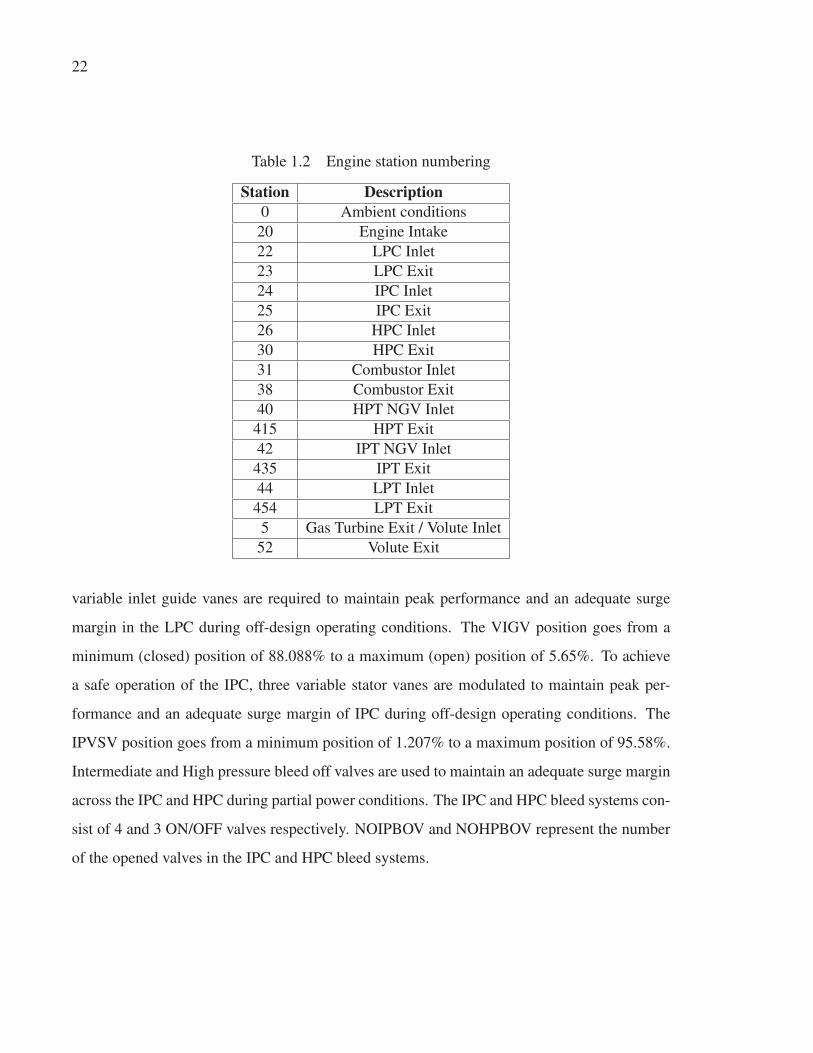
Table 1.2 Engine station numbering . . . . . . . . . . . . . . . . . . . . . . . . . . . . . . . . . . . . . . . . . . . . . . . . . . . . . . . 22
Table 3.1 Time series datasets . . . . . . . . . . . . . . . . . . . . . . . . . . . . . . . . . . . . . . . . . . . . . . . . . . . . . . . . . . . . . . 64
Table 3.2 System order and delay estimation results . . . . . . . . . . . . . . . . . . . . . . . . . . . . . . . . . . . . . . 67
Table 3.3 Summary of construction of MISO-NARX models for NH . . . . . . . . . . . . . . . . . . . 70
Table 3.4 The best MISO NARX models configuration . . . . . . . . . . . . . . . . . . . . . . . . . . . . . . . . . . 71
Table 3.5 The best MISO NARX models configuration for NH . . . . . . . . . . . . . . . . . . . . . . . . . . 74
Table 3.6 The best MISO NARX models configuration for NI . . . . . . . . . . . . . . . . . . . . . . . . . . . 75
Table 3.7 The best MISO NARX models configuration for NL . . . . . . . . . . . . . . . . . . . . . . . . . . . 76
Table 3.8 The best MISO NARX models configuration for PW . . . . . . . . . . . . . . . . . . . . . . . . . . 77
Table 3.9 The best MISO NARX models configuration for T GT . . . . . . . . . . . . . . . . . . . . . . . . 78
Table 3.10 The best MISO NARX models configuration for T30 . . . . . . . . . . . . . . . . . . . . . . . . . . 79
Table 3.11 The best MISO NARX models configuration for P30 . . . . . . . . . . . . . . . . . . . . . . . . . . 80
Table 3.12 RMSE of ensemble of MISO NARX models with different
integration methods - T S1exp . . . . . . . . . . . . . . . . . . . . . . . . . . . . . . . . . . . . . . . . . . . . . . . . . . . . 88
Table 3.13 Regression performance [RMSE] of single MISO NARX model and
ensemble of eight MISO NARX models - PW . . . . . . . . . . . . . . . . . . . . . . . . . . . . . . . . . 94
Table 3.14 Regression performance [RMSE] of single MISO NARX model and
ensemble of eight MISO NARX models - NH . . . . . . . . . . . . . . . . . . . . . . . . . . . . . . . . . . 96
Table 3.15 Regression performance [RMSE] of single MISO NARX model and
ensemble of eight MISO NARX models - NI . . . . . . . . . . . . . . . . . . . . . . . . . . . . . . . . . . 98
Table 3.16 Regression performance [RMSE] of single MISO NARX model and
ensemble of eight MISO NARX models - NL . . . . . . . . . . . . . . . . . . . . . . . . . . . . . . . . .100
Table 3.17 Regression performance [RMSE] of single MISO NARX model and
ensemble of eight MISO NARX models - T GT . . . . . . . . . . . . . . . . . . . . . . . . . . . . . .102
XIV
Table 3.18 Regression performance [RMSE] of single MISO NARX model and
ensemble of eight MISO NARX models - T30 . . . . . . . . . . . . . . . . . . . . . . . . . . . . . . . . .104
Table 3.19 Regression performance [RMSE] of single MISO NARX model and
ensemble of eight MISO NARX models - P30 . . . . . . . . . . . . . . . . . . . . . . . . . . . . . . . . .106
Table 5.1 Input and output parameters cross correlation . . . . . . . . . . . . . . . . . . . . . . . . . . . . . . . .136
Table 5.2 Input and output parameters constraints . . . . . . . . . . . . . . . . . . . . . . . . . . . . . . . . . . . . . . .137
Table 5.3 The control performance comparison with various N2 values . . . . . . . . . . . . . . . .148
Table 5.4 The controller performance comparison under load rejection test . . . . . . . . . . . .158
LIST OF FIGURES
Page
Figure 0.1 Gas turbine engine operation envelope . . . . . . . . . . . . . . . . . . . . . . . . . . . . . . . . . . . . . . . . . 2
Figure 0.2 New competitive area of gas turbine engine control system . . . . . . . . . . . . . . . . . . . 5
Figure 1.1 Gas turbine cycle and T − s and p−V diagram for Brayton cycle . . . . . . . . . . . 13
Figure 1.2 Gas turbine engine components . . . . . . . . . . . . . . . . . . . . . . . . . . . . . . . . . . . . . . . . . . . . . . . . 14
Figure 1.3 A Whittle-type turbo-jet engine . . . . . . . . . . . . . . . . . . . . . . . . . . . . . . . . . . . . . . . . . . . . . . . . 15
Figure 1.4 Types of gas turbine engines . . . . . . . . . . . . . . . . . . . . . . . . . . . . . . . . . . . . . . . . . . . . . . . . . . . 15
Figure 1.5 Turbofan engine and its aero derivative engine . . . . . . . . . . . . . . . . . . . . . . . . . . . . . . . . 17
Figure 1.6 Isochronous mode. . . . . . . . . . . . . . . . . . . . . . . . . . . . . . . . . . . . . . . . . . . . . . . . . . . . . . . . . . . . . . . 18
Figure 1.7 Droop mode . . . . . . . . . . . . . . . . . . . . . . . . . . . . . . . . . . . . . . . . . . . . . . . . . . . . . . . . . . . . . . . . . . . . . 19
Figure 1.8 Physical analogy to ADGTE with a droop mode. . . . . . . . . . . . . . . . . . . . . . . . . . . . . . 20
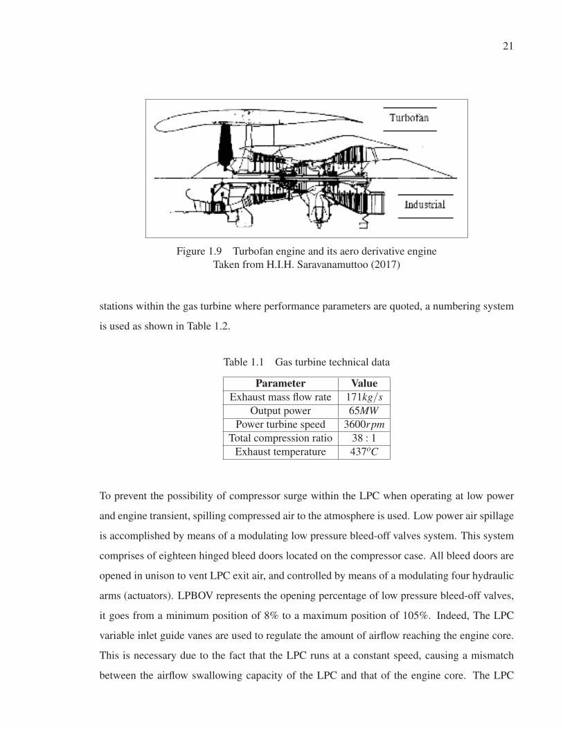
Figure 1.9 Turbofan engine and its aero derivative engine . . . . . . . . . . . . . . . . . . . . . . . . . . . . . . . . 21
Figure 1.10 Siemens SGT-A65 DLE ADGTE . . . . . . . . . . . . . . . . . . . . . . . . . . . . . . . . . . . . . . . . . . . . . . 23
Figure 1.11 Sketch of three spool aero derivative gas turbine engine (SGT-A65) . . . . . . . . 23
Figure 1.12 The SGT-A65 engine control system . . . . . . . . . . . . . . . . . . . . . . . . . . . . . . . . . . . . . . . . . . 24
Figure 1.13 The SGT-A65 engine start sequences . . . . . . . . . . . . . . . . . . . . . . . . . . . . . . . . . . . . . . . . . . 25
Figure 1.14 The axial compressor map. . . . . . . . . . . . . . . . . . . . . . . . . . . . . . . . . . . . . . . . . . . . . . . . . . . . . . 28
Figure 1.15 The compressor map and beta lines . . . . . . . . . . . . . . . . . . . . . . . . . . . . . . . . . . . . . . . . . . . . 29
Figure 1.16 An air/gas control volume . . . . . . . . . . . . . . . . . . . . . . . . . . . . . . . . . . . . . . . . . . . . . . . . . . . . . . 34
Figure 1.17 Computational flow diagram of a three spool ADGTE . . . . . . . . . . . . . . . . . . . . . . . 35
Figure 2.1 Neural network types . . . . . . . . . . . . . . . . . . . . . . . . . . . . . . . . . . . . . . . . . . . . . . . . . . . . . . . . . . . 45
Figure 2.2 History of engine control technology . . . . . . . . . . . . . . . . . . . . . . . . . . . . . . . . . . . . . . . . . . 49
Figure 2.3 Gas turbine modelling approaches . . . . . . . . . . . . . . . . . . . . . . . . . . . . . . . . . . . . . . . . . . . . . 55
XVI
Figure 2.4 Functions of the human brain . . . . . . . . . . . . . . . . . . . . . . . . . . . . . . . . . . . . . . . . . . . . . . . . . . 58
Figure 2.5 Basic neuron types . . . . . . . . . . . . . . . . . . . . . . . . . . . . . . . . . . . . . . . . . . . . . . . . . . . . . . . . . . . . . . 59
Figure 3.1 A simple structure of an ANN with input, hidden and output layers . . . . . . . . . 62
Figure 3.2 The flow diagram of the modelling approach . . . . . . . . . . . . . . . . . . . . . . . . . . . . . . . . . 63
Figure 3.3 Impulse response from WF to NH used to estimate the input-output
delay. . . . . . . . . . . . . . . . . . . . . . . . . . . . . . . . . . . . . . . . . . . . . . . . . . . . . . . . . . . . . . . . . . . . . . . . . . . . . 66
Figure 3.4 Flow diagram of the generated computer code for NARX model of
the ADGTE . . . . . . . . . . . . . . . . . . . . . . . . . . . . . . . . . . . . . . . . . . . . . . . . . . . . . . . . . . . . . . . . . . . . . 69
Figure 3.5 MISO-NARX models of SGT-A65 engine . . . . . . . . . . . . . . . . . . . . . . . . . . . . . . . . . . . . 72
Figure 3.6 MISO-NARX models of SGT-A65 engine . . . . . . . . . . . . . . . . . . . . . . . . . . . . . . . . . . . . 73
Figure 3.7 MISO-NARX model prediction and the actual engine output for
NH : (a) Training , (b) Testing . . . . . . . . . . . . . . . . . . . . . . . . . . . . . . . . . . . . . . . . . . . . . . . . . 74
Figure 3.8 MISO-NARX model prediction and the actual engine output for NI: (a) Training , (b) Testing. . . . . . . . . . . . . . . . . . . . . . . . . . . . . . . . . . . . . . . . . . . . . . . . . . . . . . 75
Figure 3.9 MISO-NARX model prediction and the actual engine output for
NL : (a) Training , (b) Testing . . . . . . . . . . . . . . . . . . . . . . . . . . . . . . . . . . . . . . . . . . . . . . . . . . 76
Figure 3.10 MISO-NARX model prediction and the actual engine output for
PW : (a) Training , (b) Testing . . . . . . . . . . . . . . . . . . . . . . . . . . . . . . . . . . . . . . . . . . . . . . . . . 77
Figure 3.11 MISO-NARX model prediction and the actual engine output for
T GT : (a) Training , (b) Testing . . . . . . . . . . . . . . . . . . . . . . . . . . . . . . . . . . . . . . . . . . . . . . . 78
Figure 3.12 MISO-NARX model prediction and the actual engine output for
T30 : (a) Training , (b) Testing . . . . . . . . . . . . . . . . . . . . . . . . . . . . . . . . . . . . . . . . . . . . . . . . . 79
Figure 3.13 MISO-NARX model prediction and the actual engine output for
P30 : (a) Training , (b) Testing . . . . . . . . . . . . . . . . . . . . . . . . . . . . . . . . . . . . . . . . . . . . . . . . . 81
Figure 3.14 Ensemble generation steps . . . . . . . . . . . . . . . . . . . . . . . . . . . . . . . . . . . . . . . . . . . . . . . . . . . . . 81
Figure 3.15 Inside of an ensemble model . . . . . . . . . . . . . . . . . . . . . . . . . . . . . . . . . . . . . . . . . . . . . . . . . . . 82
Figure 3.16 NH ensemble models prediction - T S1exp . . . . . . . . . . . . . . . . . . . . . . . . . . . . . . . . . . . . . . 83
Figure 3.17 NI ensemble models prediction - T S1exp . . . . . . . . . . . . . . . . . . . . . . . . . . . . . . . . . . . . . . 83
XVII
Figure 3.18 NL ensemble models prediction - T S1exp . . . . . . . . . . . . . . . . . . . . . . . . . . . . . . . . . . . . . . 84
Figure 3.19 PW ensemble models prediction - T S1exp . . . . . . . . . . . . . . . . . . . . . . . . . . . . . . . . . . . . . 84
Figure 3.20 T GT ensemble models prediction - T S1exp . . . . . . . . . . . . . . . . . . . . . . . . . . . . . . . . . . . 85
Figure 3.21 T30 ensemble models prediction - T S1exp . . . . . . . . . . . . . . . . . . . . . . . . . . . . . . . . . . . . . . 85
Figure 3.22 P30 ensemble models prediction - T S1exp . . . . . . . . . . . . . . . . . . . . . . . . . . . . . . . . . . . . . . 86
Figure 3.23 NHensemble regression with different integration methods - T S1exp . . . . . . . . 89
Figure 3.24 NI ensemble regression with different integration methods - T S1exp . . . . . . . . 89
Figure 3.25 NL ensemble regression with different integration methods - T S1exp . . . . . . . . 90
Figure 3.26 PW ensemble regression with different integration methods -
T S1exp . . . . . . . . . . . . . . . . . . . . . . . . . . . . . . . . . . . . . . . . . . . . . . . . . . . . . . . . . . . . . . . . . . . . . . . . . . . 90
Figure 3.27 T GT ensemble regression with different integration methods -
T S1exp . . . . . . . . . . . . . . . . . . . . . . . . . . . . . . . . . . . . . . . . . . . . . . . . . . . . . . . . . . . . . . . . . . . . . . . . . . . 91
Figure 3.28 T30 ensemble regression with different integration methods -
T S1exp . . . . . . . . . . . . . . . . . . . . . . . . . . . . . . . . . . . . . . . . . . . . . . . . . . . . . . . . . . . . . . . . . . . . . . . . . . . 91
Figure 3.29 P30 ensemble regression with different integration methods -
T S1exp . . . . . . . . . . . . . . . . . . . . . . . . . . . . . . . . . . . . . . . . . . . . . . . . . . . . . . . . . . . . . . . . . . . . . . . . . . . 92
Figure 3.30 Ensemble model of SGT-A65 engine . . . . . . . . . . . . . . . . . . . . . . . . . . . . . . . . . . . . . . . . . . 92
Figure 3.31 The comparison between the performance of ensemble of MISO
NARX models and single MISO NARX model using T S1exp to
T S4sim datasets - PW . . . . . . . . . . . . . . . . . . . . . . . . . . . . . . . . . . . . . . . . . . . . . . . . . . . . . . . . . . . 94
Figure 3.32 The comparison between the performance of ensemble of MISO
NARX models and single MISO NARX model using T S5sim to
T S8sim datasets - PW . . . . . . . . . . . . . . . . . . . . . . . . . . . . . . . . . . . . . . . . . . . . . . . . . . . . . . . . . . . 95
Figure 3.33 The comparison between the performance of ensemble of MISO
NARX models and single MISO NARX model using T S1exp to
T S4sim datasets - NH . . . . . . . . . . . . . . . . . . . . . . . . . . . . . . . . . . . . . . . . . . . . . . . . . . . . . . . . . . . . 96
Figure 3.34 The comparison between the performance of ensemble of MISO
NARX models and single MISO NARX model using T S5sim to
T S8sim datasets - NH . . . . . . . . . . . . . . . . . . . . . . . . . . . . . . . . . . . . . . . . . . . . . . . . . . . . . . . . . . . . 97
XVIII
Figure 3.35 The comparison between the performance of ensemble of MISO
NARX models and single MISO NARX model using T S1exp to
T S4sim datasets - NI . . . . . . . . . . . . . . . . . . . . . . . . . . . . . . . . . . . . . . . . . . . . . . . . . . . . . . . . . . . . 98
Figure 3.36 The comparison between the performance of ensemble of MISO
NARX models and single MISO NARX model using T S5sim to
T S8sim datasets - NI . . . . . . . . . . . . . . . . . . . . . . . . . . . . . . . . . . . . . . . . . . . . . . . . . . . . . . . . . . . . 99
Figure 3.37 The comparison between the performance of ensemble of MISO
NARX models and single MISO NARX model using T S1exp to
T S4sim datasets - NL . . . . . . . . . . . . . . . . . . . . . . . . . . . . . . . . . . . . . . . . . . . . . . . . . . . . . . . . . . .100
Figure 3.38 The comparison between the performance of ensemble of MISO
NARX models and single MISO NARX model using T S5sim to
T S8sim datasets - NL . . . . . . . . . . . . . . . . . . . . . . . . . . . . . . . . . . . . . . . . . . . . . . . . . . . . . . . . . . .101
Figure 3.39 The comparison between the performance of ensemble of MISO
NARX models and single MISO NARX model using T S1exp to
T S4sim datasets - T GT . . . . . . . . . . . . . . . . . . . . . . . . . . . . . . . . . . . . . . . . . . . . . . . . . . . . . . . .102
Figure 3.40 The comparison between the performance of ensemble of MISO
NARX models and single MISO NARX model using T S5sim to
T S8sim datasets - T GT . . . . . . . . . . . . . . . . . . . . . . . . . . . . . . . . . . . . . . . . . . . . . . . . . . . . . . . .103
Figure 3.41 The comparison between the performance of ensemble of MISO
NARX models and single MISO NARX model using T S1exp to
T S4sim datasets - T30 . . . . . . . . . . . . . . . . . . . . . . . . . . . . . . . . . . . . . . . . . . . . . . . . . . . . . . . . . . .104
Figure 3.42 The comparison between the performance of ensemble of MISO
NARX models and single MISO NARX model using T S5sim to
T S8sim datasets - T30 . . . . . . . . . . . . . . . . . . . . . . . . . . . . . . . . . . . . . . . . . . . . . . . . . . . . . . . . . . .105
Figure 3.43 The comparison between the performance of ensemble of MISO
NARX models and single MISO NARX model using T S1exp to
T S4sim datasets - P30 . . . . . . . . . . . . . . . . . . . . . . . . . . . . . . . . . . . . . . . . . . . . . . . . . . . . . . . . . . .106
Figure 3.44 The comparison between the performance of ensemble of MISO
NARX models and single MISO NARX model using T S5sim to
T S8sim datasets - P30 . . . . . . . . . . . . . . . . . . . . . . . . . . . . . . . . . . . . . . . . . . . . . . . . . . . . . . . . . . .107
Figure 4.1 The MPC Strategy . . . . . . . . . . . . . . . . . . . . . . . . . . . . . . . . . . . . . . . . . . . . . . . . . . . . . . . . . . . . .112
Figure 4.2 Block diagram of a model predictive controller . . . . . . . . . . . . . . . . . . . . . . . . . . . . . .113
Figure 4.3 Block diagram of NMPC system. . . . . . . . . . . . . . . . . . . . . . . . . . . . . . . . . . . . . . . . . . . . . .126
XIX
Figure 5.1 Engine fuel control system using min-max controller . . . . . . . . . . . . . . . . . . . . . . .134
Figure 5.2 The NNGPC for SGT-A65 . . . . . . . . . . . . . . . . . . . . . . . . . . . . . . . . . . . . . . . . . . . . . . . . . . . .136
Figure 5.3 The NNGPC SIMULINK block . . . . . . . . . . . . . . . . . . . . . . . . . . . . . . . . . . . . . . . . . . . . . .141
Figure 5.4 The Predictor block . . . . . . . . . . . . . . . . . . . . . . . . . . . . . . . . . . . . . . . . . . . . . . . . . . . . . . . . . . . .142
Figure 5.5 The free response block . . . . . . . . . . . . . . . . . . . . . . . . . . . . . . . . . . . . . . . . . . . . . . . . . . . . . . .142
Figure 5.6 The NL ensemble block . . . . . . . . . . . . . . . . . . . . . . . . . . . . . . . . . . . . . . . . . . . . . . . . . . . . . . . .143
Figure 5.7 The step response block . . . . . . . . . . . . . . . . . . . . . . . . . . . . . . . . . . . . . . . . . . . . . . . . . . . . . . .143
Figure 5.8 Integration of onboard model and actual engine model . . . . . . . . . . . . . . . . . . . . . .144
Figure 5.9 The actual engine model testing results: NH . . . . . . . . . . . . . . . . . . . . . . . . . . . . . . . . .144
Figure 5.10 The actual engine model testing results: NI . . . . . . . . . . . . . . . . . . . . . . . . . . . . . . . . . .145
Figure 5.11 The actual engine model testing results: NL . . . . . . . . . . . . . . . . . . . . . . . . . . . . . . . . . .145
Figure 5.12 The actual engine model testing results: PW . . . . . . . . . . . . . . . . . . . . . . . . . . . . . . . . .145
Figure 5.13 The actual engine model testing results: T30 . . . . . . . . . . . . . . . . . . . . . . . . . . . . . . . . .146
Figure 5.14 The actual engine model testing results: P30 . . . . . . . . . . . . . . . . . . . . . . . . . . . . . . . . .146
Figure 5.15 The actual engine model testing results: T GT . . . . . . . . . . . . . . . . . . . . . . . . . . . . . . .146
Figure 5.16 Effect of prediction horizon on PW . . . . . . . . . . . . . . . . . . . . . . . . . . . . . . . . . . . . . . . . . . .148
Figure 5.17 Effect of prediction horizon on NL . . . . . . . . . . . . . . . . . . . . . . . . . . . . . . . . . . . . . . . . . . . .149
Figure 5.18 Effect of prediction horizon on WF . . . . . . . . . . . . . . . . . . . . . . . . . . . . . . . . . . . . . . . . . . .149
Figure 5.19 Effect of prediction horizon on IPV SV . . . . . . . . . . . . . . . . . . . . . . . . . . . . . . . . . . . . . . .150
Figure 5.20 Effect of prediction horizon on LPBOV . . . . . . . . . . . . . . . . . . . . . . . . . . . . . . . . . . . . . .150
Figure 5.21 The generator load profile . . . . . . . . . . . . . . . . . . . . . . . . . . . . . . . . . . . . . . . . . . . . . . . . . . . . .151
Figure 5.22 The PW response during load change . . . . . . . . . . . . . . . . . . . . . . . . . . . . . . . . . . . . . . . .153
Figure 5.23 The NL response during load change. . . . . . . . . . . . . . . . . . . . . . . . . . . . . . . . . . . . . . . . . .153
Figure 5.24 The NH response during load change . . . . . . . . . . . . . . . . . . . . . . . . . . . . . . . . . . . . . . . . .154
XX
Figure 5.25 The NI response during load change . . . . . . . . . . . . . . . . . . . . . . . . . . . . . . . . . . . . . . . . . .154
Figure 5.26 The T GT response during load change . . . . . . . . . . . . . . . . . . . . . . . . . . . . . . . . . . . . . . .155
Figure 5.27 The P30 response during load change . . . . . . . . . . . . . . . . . . . . . . . . . . . . . . . . . . . . . . . . .155
Figure 5.28 The T30 response during load change . . . . . . . . . . . . . . . . . . . . . . . . . . . . . . . . . . . . . . . . .156
Figure 5.29 The WF response during load change . . . . . . . . . . . . . . . . . . . . . . . . . . . . . . . . . . . . . . . .156
Figure 5.30 The IPV SV response during load change . . . . . . . . . . . . . . . . . . . . . . . . . . . . . . . . . . . . .157
Figure 5.31 The LPBOV response during load change . . . . . . . . . . . . . . . . . . . . . . . . . . . . . . . . . . . .157
Figure 5.32 Comparison between NNGPC controller and min-max controller
performance during load disturbance - PW . . . . . . . . . . . . . . . . . . . . . . . . . . . . . . . . . .160
Figure 5.33 Comparison between NNGPC controller and min-max controller
performance during load disturbance - NL . . . . . . . . . . . . . . . . . . . . . . . . . . . . . . . . . . .160
Figure 5.34 Comparison between NNGPC controller and min-max controller
performance during load disturbance - NH . . . . . . . . . . . . . . . . . . . . . . . . . . . . . . . . . . .161
Figure 5.35 Comparison between NNGPC controller and min-max controller
performance during load disturbance - NI . . . . . . . . . . . . . . . . . . . . . . . . . . . . . . . . . . . .161
Figure 5.36 Comparison between NNGPC controller and min-max controller
performance during load disturbance - T GT . . . . . . . . . . . . . . . . . . . . . . . . . . . . . . . . .162
Figure 5.37 Comparison between NNGPC controller and min-max controller
performance during load disturbance - P30 . . . . . . . . . . . . . . . . . . . . . . . . . . . . . . . . . . .162
Figure 5.38 Comparison between NNGPC controller and min-max controller
performance during load disturbance - T30 . . . . . . . . . . . . . . . . . . . . . . . . . . . . . . . . . . .163
Figure 5.39 Comparison between NNGPC controller and min-max controller
performance during load disturbance - WF . . . . . . . . . . . . . . . . . . . . . . . . . . . . . . . . . .163
Figure 5.40 Comparison between NNGPC controller and min-max controller
performance during load disturbance - IPV SV . . . . . . . . . . . . . . . . . . . . . . . . . . . . . .164
Figure 5.41 Comparison between NNGPC controller and min-max controller
performance during load disturbance - LPBOV . . . . . . . . . . . . . . . . . . . . . . . . . . . . . .164
LIST OF ABREVIATIONS
ADGTE Aero-derivative gas turbine engine
GTE Gas turbine engine
DLE Dry low emission
LPC Low pressure compressor
IPC Intermediate pressure compressor
HPC High pressure compressor
LPT Low pressure turbine
IPT Intermediate pressure turbine
HPT High pressure turbine
LP Low pressure
IP Intermediate pressure
HP High pressure
PT Power turbine
CC Combustion chamber
ECS Engine control system
NGV Nozzle guide vanes
OGV outlet guide vane
CMF Constant mass flow iterative method
ICV Inter-component volume method
XXII
NN Neural network
ANN Artificial neural network
ARX Autoregressive with exogenous inputs
NARX Non-linear autoregressive with exogenous inputs
trainbr Bayesian regularization training algorithm
trainlm Levenberg-Marquardt training algorithm
trainscg Scaled conjugate gradient training algorithm
RUL Remaining useful life
MPC Model predictive control
LMPC Linear model predictive control
NMPC Non-linear model predictive control
NLP Non-linear programming
GPC Generalized predictive control
NNGPC Neural network generalized predictive control
SISO Single-input single-output
MIMO Multiple-input multiple-output
MISO Multiple-input single-output
SQP Sequential quadratic programming
HDWM Hybrid dynamic weighting method
BEM Basic ensemble method

XXIII
DWM Dynamic weighting method
QP Quadratic programming
PI Proportional plus integral
CPU Central processing unit

LISTE OF SYMBOLS AND UNITS OF MEASUREMENTS
WF Fuel flow in ppm
LPBOV Low pressure bleed-off valves position %
VIGV Variable inlet guide vanes position %
IPVSV Variable stator vanes position %
IPBOV Number of opened intermediate pressure bleed off valves
HPBOV Number of opened High pressure bleed off valves
NOx Nitrogen oxide
M Mach number
B Bleed fraction
LHV Fuel heating value
N Relative spool speed
T Stagnation temperature
P Stagnation pressure
W Work
WT Work of turbine
WC Work of compressor
PWdem Power demand
U Internal energy
f Frequency
XXVI
H Altitude
J Polar moment of inertia
cpa Specific heat at constant pressure of air
cpg Specific heat at constant pressure of gas
cv Specific heat at constant volume
ΔPRin Inlet pressure losses
ΔPRCC Combustor pressure losses
ΔPRex Exhaust nozzle pressure losses
γa Specific heat ratio of air
γg Specific heat ratio of combustion gas
R Universal gas constant
β Beta value
ηth Thermal efficiency
θ Corrected temperature
δ Corrected pressure
π Pressure ratio
m• Mass flow rate
d Droop percentage of the engine generator
y The predicted output
w The reference output

XXVII
u The Manipulated input
N2 The maximum prediction horizon
N1 The minimum predictive horizon
Nu The control horizon
Ts The sampling time
Λ The control-weighting factor
λ The Lagrangian multiplier
yyyconstr The constraint output vector
ycontr The controlled output vector
kg Kilogram
s Second
ms Milliseconds
K Kelvin
MW Mega watt
ppm Parts per million
pph Pounds per hour
rpm Revolution per minute
Hz Hertz
T • The rate of change of temperature
P• The rate of change of pressure
U• The rate of change of internal energy

INTRODUCTION
Gas Turbine is a complex system with highly nonlinear dynamics and a large operating range.
Gas turbine engines and their related technologies represent one of the most efficient forms
of propulsion and power generation, with applications in various areas: as prime movers in
planes, in power plants for electricity generation, ground-based vehicle and marine ships for
propulsion. Increasing demands for gas turbine engines usage in many fields have caused
different design requirements such as, improving performance, more efficiency, reliability, and
the reduction of development costs and time. As a result, the cost of research, development and
implementation of new technology in gas turbine systems is becoming prohibitively expensive.
Moreover, one of the main reasons of this high development cost is the need to perform many
hardware tests of the physical engine. Therefore, the needs for exploring the performance
of gas turbine engines to reduce the initial cost of designing new engines and improve the
performance has led to the raise of research on modelling and simulation of gas turbine engines.
Effective simulation models can be developed without any prototypes being needed at the very
early stages of the design. In addition, modelling of gas turbine engines can be used in the
design of engine’s controller. Based on the fact that gas turbine engines are highly non-linear
and operate very close to their thermal and mechanical limits, many layers of complexity are
added to the controller design operation which emphasizes the need for sophisticated control
systems. Also, modifications to the control system become the desired path in the development
field of gas turbines because it is easier to change the control logic and the corresponding code
rather than to redesign, re-manufacture, and reinstall new engine components. The objective of
the control system is to achieve good thrust or shaft power response qualities while maintaining
critical engine outputs within safety limits. The design of controllers capable of delivering this
objective represents a challenging problem (Richter, 2011).
2
Problem Statement
Gas turbine engine, as mentioned above, is a highly non-linear plant due to the large range
of operation conditions and the power levels experienced during a typical mission. Also gas
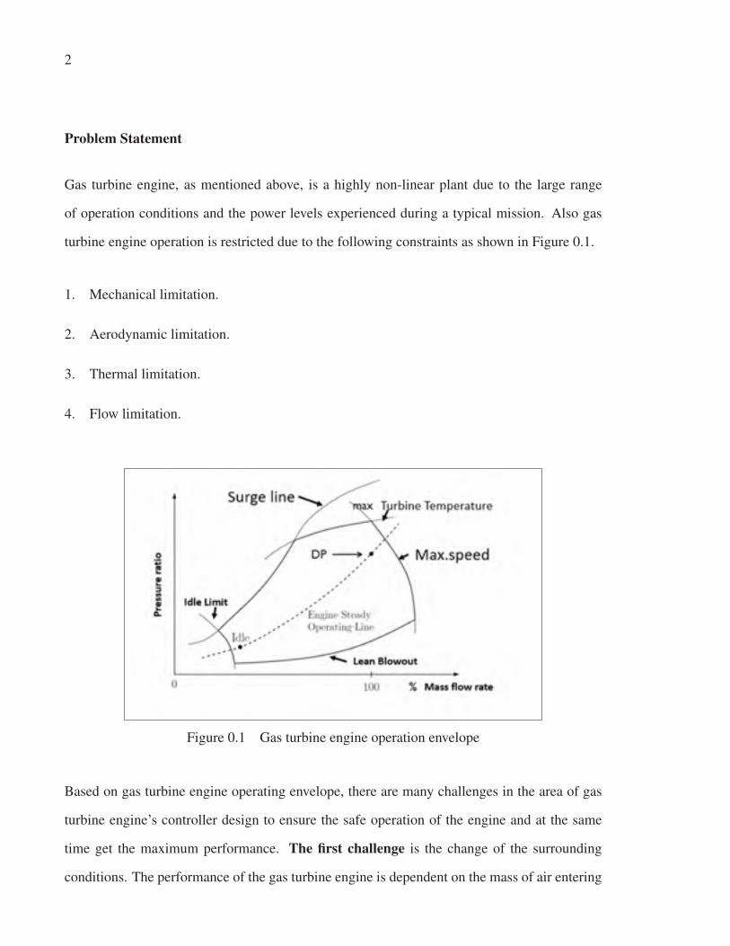
turbine engine operation is restricted due to the following constraints as shown in Figure 0.1.
1. Mechanical limitation.
2. Aerodynamic limitation.
3. Thermal limitation.
4. Flow limitation.
Figure 0.1 Gas turbine engine operation envelope
Based on gas turbine engine operating envelope, there are many challenges in the area of gas
turbine engine’s controller design to ensure the safe operation of the engine and at the same
time get the maximum performance. The first challenge is the change of the surrounding
conditions. The performance of the gas turbine engine is dependent on the mass of air entering

3
the engine. At a constant speed, the compressor pumps a constant volume of air into the engine
with no regard for air mass or density. If the density of the air decreases, the same volume of
air will contain less mass, so less power is produced. If air density increases, power output also
increases as the air mass flow increases for the same volume of air. Atmospheric conditions
affect the performance of the engine since the density of the air will be different under different
conditions [−60oC to 40oC air temperature]. On a cold day, the air density is high, so the mass
of the air entering the compressor is increased. As a result, higher horsepower is produced. In
contrast, on a hot day, or at high altitude, air density is decreased, resulting in a decrease of
output shaft power.
The second challenge is quick engine start. Quick engine starts and rapid accelerations are
also desirable. To provide higher power with low specific fuel consumption and acceptable
starting and acceleration characteristics, it is necessary to operate as close to the surge region
as possible. To prevent compressor stall or surge, fuel flow must be properly metered during
the start and acceleration cycle of any gas turbine engine. To accomplish this, we need a very
accurate engine controller.
The third challenge: On the emissions side, the challenge is to increase turbine inlet temper-
atures while at the same time reduce peak flame temperature in order to achieve lower NOx
emissions and meet the latest emission regulations. In addition, reliable fuel switching capa-
bilities in industrial gas turbine engines should be taken in consideration.
The fourth challenge: With respect to components lifetime, and performance degradation,
there are big challenges in this area because customers need to increase components lifetime in
order to decrease the cost but at the same time ensure the safe, reliable and high performance
of the engine operation. Therefore, these requirements put more complexity on the design
operation of the gas turbine engine controller. In addition, every gas turbine engine has its
own signature even for the same engine’s configuration over time. The gas turbine engine

4
controller should take into consideration the effect of performance degradation due to repair
and maintenance of the engine.The controller must therefore be re-tuned after any maintenance
operation to recover the engine performance. Customers needs this tuning operation of the
engine controller to be automated to save time and money and have high engine performance
at the same time.
The fifth challenge: The engine control system must handle some engine monitoring func-
tions. Traditionally, engine monitoring functions have been a part of the modern control system
functionality. To monitor engine health state and maintain high engine availability, an engine
monitoring system must be able to detect incipient failures and predict how much longer the
engine can operate with the "known" degradation before the failure becomes so severe that the
engine performance becomes unacceptable (Jaw & Mattingly, 2009).
The concept of a more intelligent gas turbine engine aims at actively controlling engine opera-
tion to increase efficiency, durability and safety, while maintaining the high level of reliability
required for aeronautic and industrial applications. Today engine manufacturers are investigat-
ing the potential of intelligent technologies for the next engine generation to meet the previous
challenges. The design of controllers capable of satisfying the previous requirements represents
a challenging problem (Figure 0.2) ; classical feedback is no longer suitable as a paradigm for
the development of advanced propulsion control concepts.
Research objectives
The research project is based on Siemens requirements, which include:
1. Real-time model based control.
5
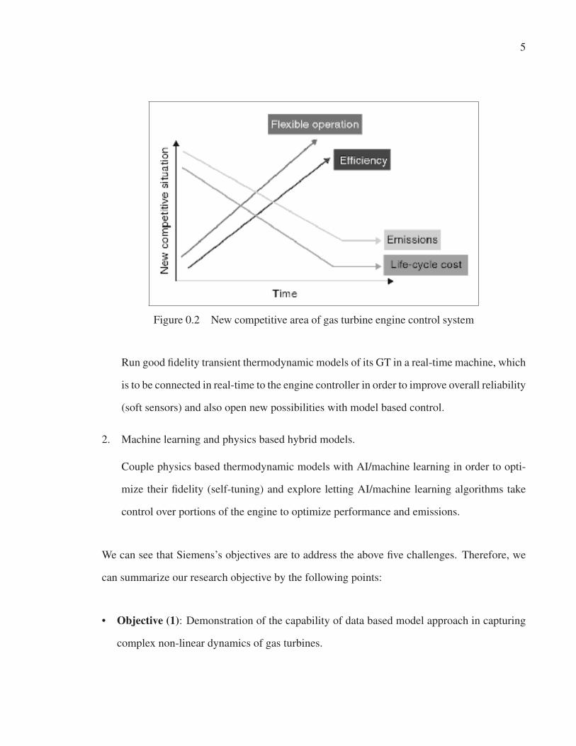
Figure 0.2 New competitive area of gas turbine engine control system
Run good fidelity transient thermodynamic models of its GT in a real-time machine, which
is to be connected in real-time to the engine controller in order to improve overall reliability
(soft sensors) and also open new possibilities with model based control.
2. Machine learning and physics based hybrid models.
Couple physics based thermodynamic models with AI/machine learning in order to opti-
mize their fidelity (self-tuning) and explore letting AI/machine learning algorithms take
control over portions of the engine to optimize performance and emissions.
We can see that Siemens’s objectives are to address the above five challenges. Therefore, we
can summarize our research objective by the following points:
• Objective (1): Demonstration of the capability of data based model approach in capturing
complex non-linear dynamics of gas turbines.

6
• Objective (2): Development of advanced controller based on good fidelity transient models
of Gas Turbines (GT) in order to improve the performance and overall reliability of the
machine.
• Objective (3): Implementation of these benefits in real time using working prototypes of
Siemens GT and their edge-computing platform.
Methodology
Different approaches are used and proposed throughout this thesis. In the following, the main
methodologies are categorized:
1. To address objective 1, Chapter 3 presents a novel data-driven neural networks based
model approach, which is used for modelling of a three-spool aero-derivative gas turbine
engine (ADGTE) used for power generation during its loading and unloading conditions.
An ensemble of MISO NARX models is used to develop this model in MATLAB environ-
ment using operational closed-loop data collected from Siemens (SGT-A65) ADGTE. The
following procedure is used during the modelling operation:
a. Data preprocessing and estimation of the order of these MISO models were per-
formed.
b. A computer program code was developed to perform a comparative study and to
select the best NARX model configuration, which can represent the system dynamics.
c. The most accurate MISO-NARX model with minimum RMSE during testing opera-
tion is selected.
d. A homogeneous ensemble for each output parameter of the engine is generated based
on the best selected structure of the MISO-NARX model from the last step, and diver-

7
sity among them is ensured by altering the training datasets which represent different
operation conditions.
e. The major challenge of the ensemble generation is to decide how to combine re-
sults produced by the ensemble’s components. In this study, a novel hybrid dynamic
weighting method (HDWM) is proposed. The verification of this method was per-
formed by comparing its performance with three of the most popular basic methods
for ensemble integration: basic ensemble method (BEM), median rule, and dynamic
weighting method (DWM).
f. Finally, the generated ensembles of MISO NARX models for each output parameter
were evaluated using unseen data (testing data).
2. To address objective 2, Chapter 4 presents a novel approach to implement the constrained
MIMO NMPC based on neural network model. The implementation of NMPC of ADGTE
in real time has two challenges: Firstly, the design of an accurate non-linear model which
can run many times faster than real time. Secondly, the usage of a rapid and reliable
optimization algorithm to solve the optimization problem in real time. To solve these
issues, the following approaches are proposed:
a. The NN model of the engine obtained using methodology 1 presented above was
used as a base model of the NMPC to predict the process output. As shown in the
results from Step 1-f of methodology 1, the ensemble of MISO-NARX models can
represent the ADGTE during the full operating range with good accuracy even with
different input scenarios from different operation conditions. This proves the high
generalization characteristic of the ensemble. Also, another important gain was the
very low execution time, which can support many real time applications like model
based controller design.

8
b. A constrained MIMO NMPC is developed based on the generalized predictive control
(GPC) algorithm because of its simplicity, ease of use, and ability to handle problems
in one algorithm. The usage of a non-linear model within GPC changes the optimiza-
tion problem from a convex quadratic problem to a nonconvex non-linear one. As
a consequence of that, there is no guarantee that the global optimum can be found
especially in real-time control when the optimum solution has to be obtained in a
prescribed time. To overcome this issue, a novel trade-off approach between the us-
age of a non-linear model and successive linearization approaches is used in order to
reduce the computation effort and at the same time increase the robustness of the con-
troller. Estimation of the free and forced responses of the GPC are performed based
on the NN model of the plant each sampling time. It reduces the neural network gen-
eralized predictive control (NNGPC) optimization problem to a linear optimization
problem at each sampling step. Therefore, the optimization problem can be solved us-
ing quadratic programming which will improve the computation time and reliability
of the solution.
c. The Hildreth’s Quadratic Programming (QP) procedure is utilized to solve the quadratic
optimization problem of the NNGPC controller, which offers simplicity and relia-
bility in real-time implementation. The maximum number of iterations within this
algorithm is calculated by trial and error and is limited to 100 iterations to avoid in-
creasing of computation time. This implies that in some cases the optimum solution
may not be reached and the algorithm will use a suboptimal solution.
d. The NNGPC tuning parameters have a great effect on the performance and computa-
tion effort of the controller. The computation effort decreases with the decrease in the
prediction horizon. However, the response speed and the computation effort increase
with increasing prediction horizon. Consequently, a trade-off is required to find the
9
effective values of the tuning parameters. In this study, a trial and error method is
employed to find the best values of the tuning parameters.
3. To address objective 3, Chapter 5 presents a comparison between the performance of the
NNGPC controller developed in this study and the existing min-max controller of the
engine and is performed to demonstrate the effectiveness of this advanced controller. This
test is performed in MATLAB/Simulink environment. As a result of the current epidemic
(Covid-19) situation, implementation of the NNGPC controller in real time using working
prototypes of Siemens GT and their edge-computing platform is replaced by validation in
MATLAB/Simulink environment using experimental data.
Thesis Contribution
Guided by the research objectives and using the methodologies proposed above, this thesis
presents the following important and novel contributions:
1. Proposing a novel methodology for the development of data driven based model of ADGTE,
in order to simulate the dynamic performance of the ADGTE during the full operating
range in real time. Inspired by the way biological neural networks process information
and by their structure which changes depending on their function, MISO NARX models
with different configurations were used to represent each of the ADGTE output parameters
with the same input parameters.
2. Proposing a novel approach for the real time performance prediction of ADGTE through
system identification using ensemble methods.
3. Proposing a novel hybrid dynamic weighting method (HDWM) to combine results pro-
duced by the ensemble’s components.

10
4. Proposing a novel approach to implement the constrained MIMO NMPC based on en-
semble of neural network models, in order to control an ADGTE during its loading and
unloading conditions.
5. Proposing a novel method to estimate the free and forced responses of the GPC based on
the NN model of the plant each sampling time. It reduces the NNGPC optimization prob-
lem to a linear optimization problem at each sampling step and improves the computation
time and reliability of the solution.
6. Using Hildreth’s quadratic programming algorithm to solve the quadratic optimization
problem within the NNGPC controller, which offers simplicity and reliability in real-time
implementation. Furthermore, Hildreth’s method may be useful to implement on non-PC
platforms like programmable logic controllers or embedded machine which do not support
linear algebra libraries.
Outline of the thesis
This thesis consists of five Chapters. Chapter 1 presents the basic aero-thermodynamic princi-
ples of gas turbines in general, and of ADGTEs in particular. It also includes the mathematical
model of a three spool SGT-A65 Siemens ADGTE used for power generation. Chapter 2
presents a comprehensive overview of the most significant researches in the field of modelling,
simulation and control of ADGTEs. It covers both physics based and data driven based models
of ADGTEs. In addition, it presents a survey of the historical development of GTE control and
the most significant publications in the field of advanced controller design for industrial GTEs.
In Chapter 3, a novel data-driven neural networks based model approach is used for mod-
elling of a three-spool aero-derivative gas turbine engine (ADGTE) used for power generation
during its loading and unloading conditions. An ensemble of MISO NARX models is used
to develop this model in MATLAB environment using operational closed-loop data collected

11
from Siemens (SGT-A65) ADGTE. Chapter 4 provides a novel approach for the design of a
constrained MIMO NMPC based on neural networks. Chapter 5 presents the development of
NNGPC controller for the three spool SGT-A65 ADGTE based on ensembles of MISO NARX
models of that engine. Finally, the conclusion and suggestions for future work are presented at
the end of the thesis.

CHAPTER 1
GAS TURBINE - OVERVIEW
1.1 Introduction
This chapter provides an overview of gas turbine engine technology and principle of oper-
ation with reference to several research publications in this field. Firstly, the basic aero-
thermodynamic principles of gas turbines in general and in particular that of ADGTEs are
introduced. This includes the mathematical model of Siemens SGT-A65 three spool ADGTE
used for power generation.
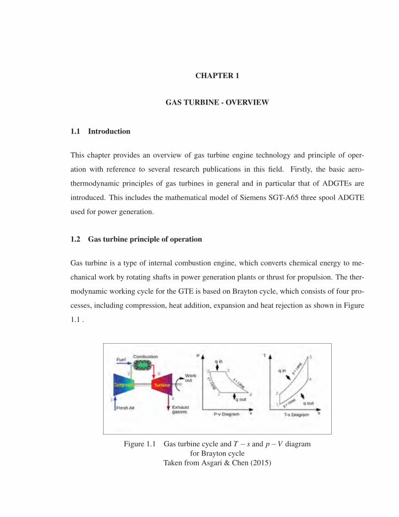
1.2 Gas turbine principle of operation
Gas turbine is a type of internal combustion engine, which converts chemical energy to me-
chanical work by rotating shafts in power generation plants or thrust for propulsion. The ther-
modynamic working cycle for the GTE is based on Brayton cycle, which consists of four pro-
cesses, including compression, heat addition, expansion and heat rejection as shown in Figure
1.1 .
Figure 1.1 Gas turbine cycle and T − s and p−V diagram
for Brayton cycle
Taken from Asgari & Chen (2015)
14
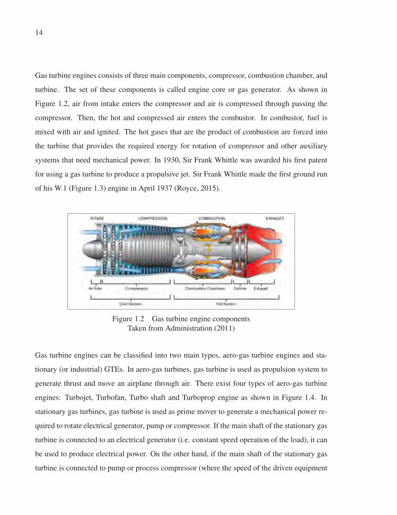
Gas turbine engines consists of three main components, compressor, combustion chamber, and
turbine. The set of these components is called engine core or gas generator. As shown in
Figure 1.2, air from intake enters the compressor and air is compressed through passing the
compressor. Then, the hot and compressed air enters the combustor. In combustor, fuel is
mixed with air and ignited. The hot gases that are the product of combustion are forced into
the turbine that provides the required energy for rotation of compressor and other auxiliary
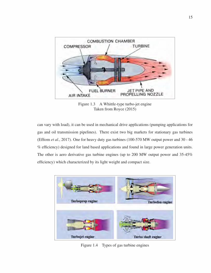
systems that need mechanical power. In 1930, Sir Frank Whittle was awarded his first patent
for using a gas turbine to produce a propulsive jet. Sir Frank Whittle made the first ground run
of his W.1 (Figure 1.3) engine in April 1937 (Royce, 2015).
Figure 1.2 Gas turbine engine components
Taken from Administration (2011)
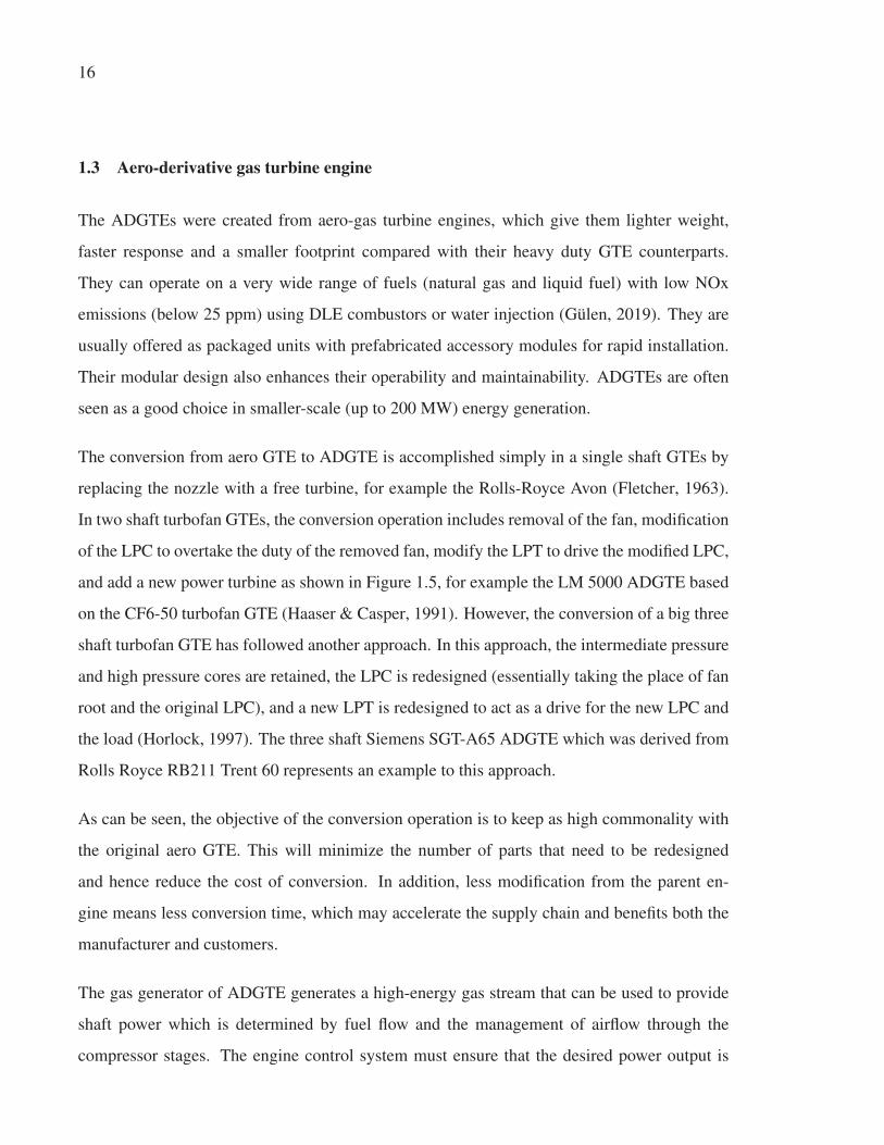
Gas turbine engines can be classified into two main types, aero-gas turbine engines and sta-
tionary (or industrial) GTEs. In aero-gas turbines, gas turbine is used as propulsion system to
generate thrust and move an airplane through air. There exist four types of aero-gas turbine
engines: Turbojet, Turbofan, Turbo shaft and Turboprop engine as shown in Figure 1.4. In
stationary gas turbines, gas turbine is used as prime mover to generate a mechanical power re-
quired to rotate electrical generator, pump or compressor. If the main shaft of the stationary gas
turbine is connected to an electrical generator (i.e. constant speed operation of the load), it can
be used to produce electrical power. On the other hand, if the main shaft of the stationary gas
turbine is connected to pump or process compressor (where the speed of the driven equipment
15
Figure 1.3 A Whittle-type turbo-jet engine
Taken from Royce (2015)
can vary with load), it can be used in mechanical drive applications (pumping applications for
gas and oil transmission pipelines). There exist two big markets for stationary gas turbines
(Effiom et al., 2017). One for heavy duty gas turbines (100-570 MW output power and 30 - 46
% efficiency) designed for land based applications and found in large power generation units.
The other is aero derivative gas turbine engines (up to 200 MW output power and 35-45%
efficiency) which characterized by its light weight and compact size.
Figure 1.4 Types of gas turbine engines
16
1.3 Aero-derivative gas turbine engine
The ADGTEs were created from aero-gas turbine engines, which give them lighter weight,
faster response and a smaller footprint compared with their heavy duty GTE counterparts.
They can operate on a very wide range of fuels (natural gas and liquid fuel) with low NOx
emissions (below 25 ppm) using DLE combustors or water injection (Gülen, 2019). They are
usually offered as packaged units with prefabricated accessory modules for rapid installation.
Their modular design also enhances their operability and maintainability. ADGTEs are often
seen as a good choice in smaller-scale (up to 200 MW) energy generation.
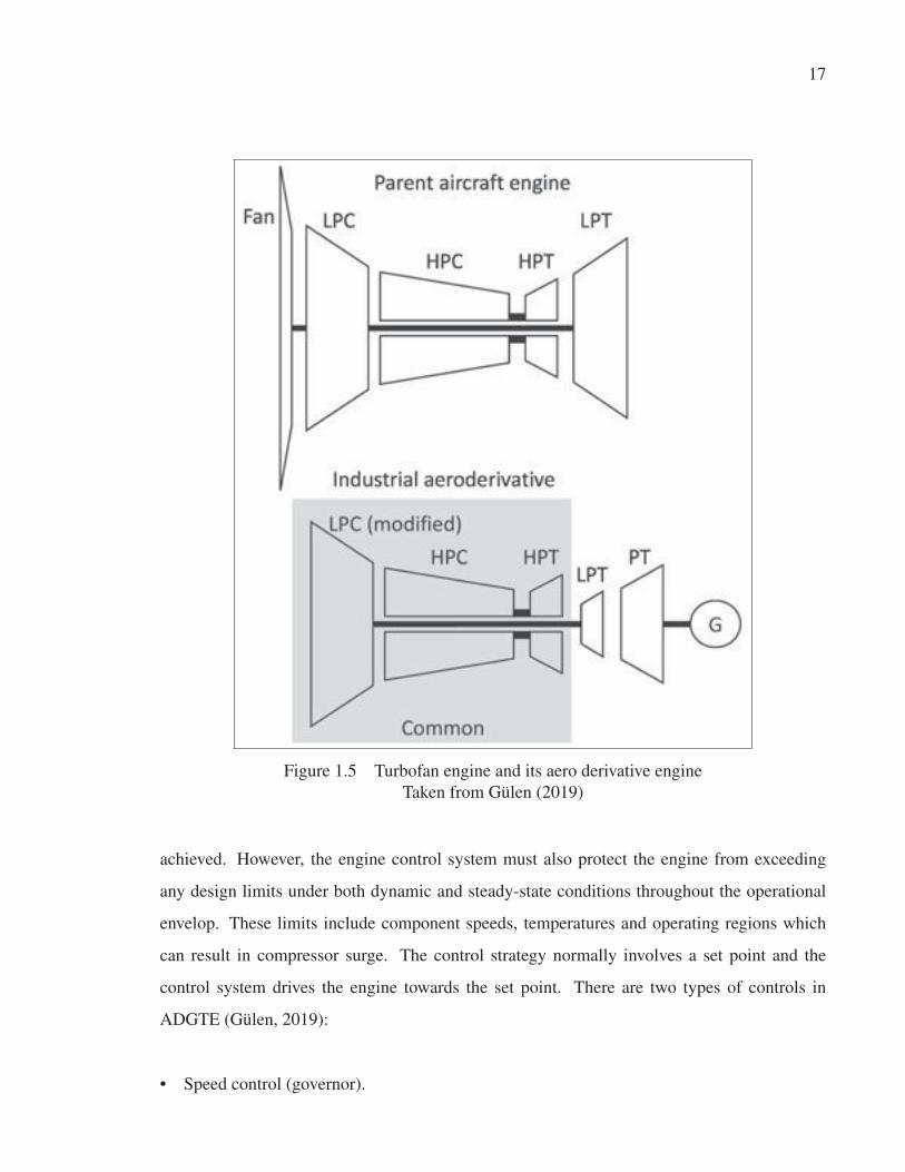
The conversion from aero GTE to ADGTE is accomplished simply in a single shaft GTEs by
replacing the nozzle with a free turbine, for example the Rolls-Royce Avon (Fletcher, 1963).
In two shaft turbofan GTEs, the conversion operation includes removal of the fan, modification
of the LPC to overtake the duty of the removed fan, modify the LPT to drive the modified LPC,
and add a new power turbine as shown in Figure 1.5, for example the LM 5000 ADGTE based
on the CF6-50 turbofan GTE (Haaser & Casper, 1991). However, the conversion of a big three
shaft turbofan GTE has followed another approach. In this approach, the intermediate pressure
and high pressure cores are retained, the LPC is redesigned (essentially taking the place of fan
root and the original LPC), and a new LPT is redesigned to act as a drive for the new LPC and
the load (Horlock, 1997). The three shaft Siemens SGT-A65 ADGTE which was derived from
Rolls Royce RB211 Trent 60 represents an example to this approach.
As can be seen, the objective of the conversion operation is to keep as high commonality with
the original aero GTE. This will minimize the number of parts that need to be redesigned
and hence reduce the cost of conversion. In addition, less modification from the parent en-
gine means less conversion time, which may accelerate the supply chain and benefits both the
manufacturer and customers.
The gas generator of ADGTE generates a high-energy gas stream that can be used to provide
shaft power which is determined by fuel flow and the management of airflow through the
compressor stages. The engine control system must ensure that the desired power output is
17
Figure 1.5 Turbofan engine and its aero derivative engine
Taken from Gülen (2019)
achieved. However, the engine control system must also protect the engine from exceeding
any design limits under both dynamic and steady-state conditions throughout the operational
envelop. These limits include component speeds, temperatures and operating regions which
can result in compressor surge. The control strategy normally involves a set point and the
control system drives the engine towards the set point. There are two types of controls in
ADGTE (Gülen, 2019):
• Speed control (governor).
18
• Temperature control.
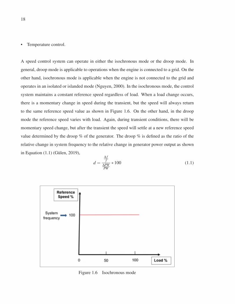
A speed control system can operate in either the isochronous mode or the droop mode. In
general, droop mode is applicable to operations when the engine is connected to a grid. On the
other hand, isochronous mode is applicable when the engine is not connected to the grid and
operates in an isolated or islanded mode (Nguyen, 2000). In the isochronous mode, the control
system maintains a constant reference speed regardless of load. When a load change occurs,
there is a momentary change in speed during the transient, but the speed will always return
to the same reference speed value as shown in Figure 1.6. On the other hand, in the droop
mode the reference speed varies with load. Again, during transient conditions, there will be
momentary speed change, but after the transient the speed will settle at a new reference speed
value determined by the droop % of the generator. The droop % is defined as the ratio of the
relative change in system frequency to the relative change in generator power output as shown
in Equation (1.1) (Gülen, 2019),
d =
Δ ff
ΔPWPW
∗100 (1.1)
Figure 1.6 Isochronous mode
19
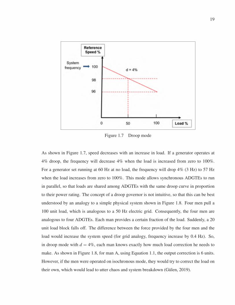
Figure 1.7 Droop mode
As shown in Figure 1.7, speed decreases with an increase in load. If a generator operates at
4% droop, the frequency will decrease 4% when the load is increased from zero to 100%.
For a generator set running at 60 Hz at no load, the frequency will drop 4% (3 Hz) to 57 Hz
when the load increases from zero to 100%. This mode allows synchronous ADGTEs to run
in parallel, so that loads are shared among ADGTEs with the same droop curve in proportion
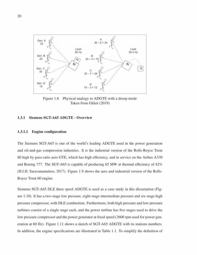
to their power rating. The concept of a droop governor is not intuitive, so that this can be best
understood by an analogy to a simple physical system shown in Figure 1.8. Four men pull a
100 unit load, which is analogous to a 50 Hz electric grid. Consequently, the four men are
analogous to four ADGTEs. Each man provides a certain fraction of the load. Suddenly, a 20
unit load block falls off. The difference between the force provided by the four men and the
load would increase the system speed (for grid analogy, frequency increase by 0.4 Hz). So,
in droop mode with d = 4%, each man knows exactly how much load correction he needs to
make. As shown in Figure 1.8, for man A, using Equation 1.1, the output correction is 6 units.
However, if the men were operated on isochronous mode, they would try to correct the load on
their own, which would lead to utter chaos and system breakdown (Gülen, 2019).
20
Figure 1.8 Physical analogy to ADGTE with a droop mode
Taken from Gülen (2019)
1.3.1 Siemens SGT-A65 ADGTE - Overview
1.3.1.1 Engine configuration
The Siemens SGT-A65 is one of the world’s leading ADGTE used in the power generation
and oil-and-gas compression industries. It is the industrial version of the Rolls-Royce Trent
60 high by-pass-ratio aero GTE, which has high efficiency, and in service on the Airbus A330
and Boeing 777. The SGT-A65 is capable of producing 65 MW at thermal efficiency of 42%
(H.I.H. Saravanamuttoo, 2017). Figure 1.9 shows the aero and industrial version of the Rolls-
Royce Trent 60 engine.
Siemens SGT-A65 DLE three spool ADGTE is used as a case study in this dissertation (Fig-
ure 1.10). It has a two-stage low pressure, eight-stage intermediate pressure and six-stage high
pressure compressor, with DLE combustion. Furthermore, both high pressure and low pressure
turbines consist of a single stage each, and the power turbine has five stages used to drive the
low pressure compressor and the power generator at fixed speed (3600 rpm used for power gen-
eration at 60 Hz). Figure 1.11 shows a sketch of SGT-A65 ADGTE with its stations numbers.
In addition, the engine specifications are illustrated in Table 1.1. To simplify the definition of
21
Figure 1.9 Turbofan engine and its aero derivative engine
Taken from H.I.H. Saravanamuttoo (2017)
stations within the gas turbine where performance parameters are quoted, a numbering system
is used as shown in Table 1.2.
Table 1.1 Gas turbine technical data
Parameter ValueExhaust mass flow rate 171kg/s
Output power 65MWPower turbine speed 3600rpm
Total compression ratio 38 : 1
Exhaust temperature 437oC
To prevent the possibility of compressor surge within the LPC when operating at low power
and engine transient, spilling compressed air to the atmosphere is used. Low power air spillage
is accomplished by means of a modulating low pressure bleed-off valves system. This system
comprises of eighteen hinged bleed doors located on the compressor case. All bleed doors are
opened in unison to vent LPC exit air, and controlled by means of a modulating four hydraulic
arms (actuators). LPBOV represents the opening percentage of low pressure bleed-off valves,
it goes from a minimum position of 8% to a maximum position of 105%. Indeed, The LPC
variable inlet guide vanes are used to regulate the amount of airflow reaching the engine core.
This is necessary due to the fact that the LPC runs at a constant speed, causing a mismatch
between the airflow swallowing capacity of the LPC and that of the engine core. The LPC
22
Table 1.2 Engine station numbering
Station Description0 Ambient conditions
20 Engine Intake
22 LPC Inlet
23 LPC Exit
24 IPC Inlet
25 IPC Exit
26 HPC Inlet
30 HPC Exit
31 Combustor Inlet
38 Combustor Exit
40 HPT NGV Inlet
415 HPT Exit
42 IPT NGV Inlet
435 IPT Exit
44 LPT Inlet
454 LPT Exit
5 Gas Turbine Exit / Volute Inlet
52 Volute Exit
variable inlet guide vanes are required to maintain peak performance and an adequate surge
margin in the LPC during off-design operating conditions. The VIGV position goes from a
minimum (closed) position of 88.088% to a maximum (open) position of 5.65%. To achieve
a safe operation of the IPC, three variable stator vanes are modulated to maintain peak per-
formance and an adequate surge margin of IPC during off-design operating conditions. The
IPVSV position goes from a minimum position of 1.207% to a maximum position of 95.58%.
Intermediate and High pressure bleed off valves are used to maintain an adequate surge margin
across the IPC and HPC during partial power conditions. The IPC and HPC bleed systems con-
sist of 4 and 3 ON/OFF valves respectively. NOIPBOV and NOHPBOV represent the number
of the opened valves in the IPC and HPC bleed systems.
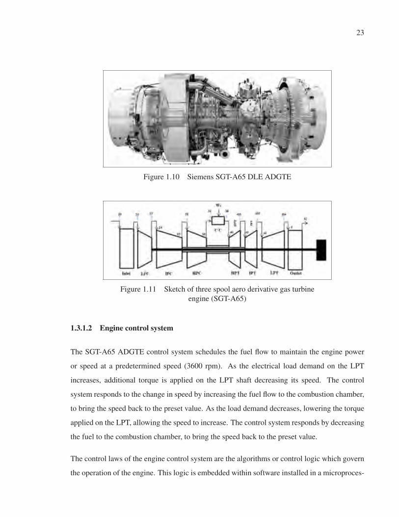
23
Figure 1.10 Siemens SGT-A65 DLE ADGTE
Figure 1.11 Sketch of three spool aero derivative gas turbine
engine (SGT-A65)
1.3.1.2 Engine control system
The SGT-A65 ADGTE control system schedules the fuel flow to maintain the engine power
or speed at a predetermined speed (3600 rpm). As the electrical load demand on the LPT
increases, additional torque is applied on the LPT shaft decreasing its speed. The control
system responds to the change in speed by increasing the fuel flow to the combustion chamber,
to bring the speed back to the preset value. As the load demand decreases, lowering the torque
applied on the LPT, allowing the speed to increase. The control system responds by decreasing
the fuel to the combustion chamber, to bring the speed back to the preset value.
The control laws of the engine control system are the algorithms or control logic which govern
the operation of the engine. This logic is embedded within software installed in a microproces-
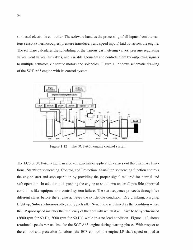
24
sor based electronic controller. The software handles the processing of all inputs from the var-
ious sensors (thermocouples, pressure transducers and speed inputs) laid out across the engine.
The software calculates the scheduling of the various gas metering valves, pressure regulating
valves, vent valves, air valves, and variable geometry and controls them by outputting signals
to multiple actuators via torque motors and solenoids. Figure 1.12 shows schematic drawing
of the SGT-A65 engine with its control system.
Figure 1.12 The SGT-A65 engine control system
The ECS of SGT-A65 engine in a power generation application carries out three primary func-
tions: Start/stop sequencing, Control, and Protection. Start/Stop sequencing function controls
the engine start and stop operation by providing the proper signal required for normal and
safe operation. In addition, it is pushing the engine to shut down under all possible abnormal
conditions like equipment or control system failure. The start sequence proceeds through five
different states before the engine achieves the synch-idle condition: Dry cranking, Purging,
Light up, Sub-synchronous idle, and Synch idle. Synch idle is defined as the condition where
the LP spool speed matches the frequency of the grid with which it will have to be synchronised
(3600 rpm for 60 Hz, 3000 rpm for 50 Hz) while in a no load condition. Figure 1.13 shows
rotational speeds versus time for the SGT-A65 engine during starting phase. With respect to
the control and protection functions, the ECS controls the engine LP shaft speed or load at
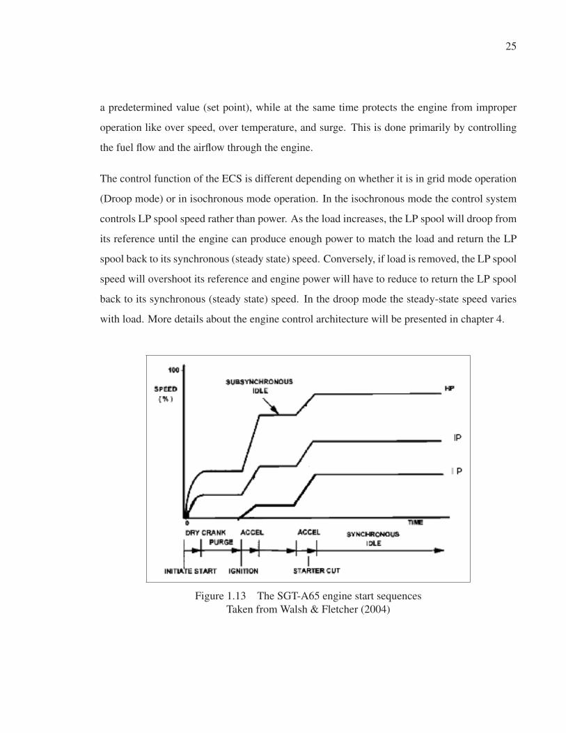
25
a predetermined value (set point), while at the same time protects the engine from improper
operation like over speed, over temperature, and surge. This is done primarily by controlling
the fuel flow and the airflow through the engine.
The control function of the ECS is different depending on whether it is in grid mode operation
(Droop mode) or in isochronous mode operation. In the isochronous mode the control system
controls LP spool speed rather than power. As the load increases, the LP spool will droop from
its reference until the engine can produce enough power to match the load and return the LP
spool back to its synchronous (steady state) speed. Conversely, if load is removed, the LP spool
speed will overshoot its reference and engine power will have to reduce to return the LP spool
back to its synchronous (steady state) speed. In the droop mode the steady-state speed varies
with load. More details about the engine control architecture will be presented in chapter 4.
Figure 1.13 The SGT-A65 engine start sequences
Taken from Walsh & Fletcher (2004)

26
1.3.2 SGT-A65 ADGTE mathematical model
This section presents the mathematical model of Siemens SGT-A65 three spool ADGTE. Al-
though this research is based on the data-driven approaches, part of the data used for the pur-
pose of simulations is generated by Siemens high fidelity thermodynamic simulation program.
Thus, it is necessary to review the engine mathematical model.
The ADGTE consists of several key components such as:
• Inlet.
• Compressor.
• Combustor.
• Gas generator turbine.
• Power turbine.
• Exhaust nozzle.
A detailed description of each of these components and ways to model them will be covered in
the following parts. In addition, the steady state and transient model will be included.
1.3.2.1 Inlet
The purpose of the engine intake is to transform the inlet free stream flow conditions into
the required air conditions at the entrance to the engine compressor. The inlet component is
assumed to be a duct and no work was done on the flow through this duct. In addition, the
performance of the inlet is defined by the pressure recovery from the free stream to the engine
(inlet pressure losses). For a given input parameters to the inlet component P0 , T0, and ΔPRin,
the total temperature and pressure at the inlet component exit are calculated as shown in the
following equations,
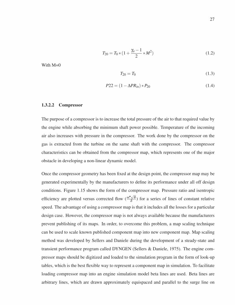
27
T20 = T0 ∗ (1+ γa −1
2∗M2) (1.2)
With M=0
T20 = T0 (1.3)
P22 = (1−ΔPRin)∗P20 (1.4)
1.3.2.2 Compressor
The purpose of a compressor is to increase the total pressure of the air to that required value by
the engine while absorbing the minimum shaft power possible. Temperature of the incoming
air also increases with pressure in the compressor. The work done by the compressor on the
gas is extracted from the turbine on the same shaft with the compressor. The compressor
characteristics can be obtained from the compressor map, which represents one of the major
obstacle in developing a non-linear dynamic model.
Once the compressor geometry has been fixed at the design point, the compressor map may be
generated experimentally by the manufacturers to define its performance under all off design
conditions. Figure 1.15 shows the form of the compressor map. Pressure ratio and isentropic
efficiency are plotted versus corrected flow (m•√θδ ) for a series of lines of constant relative
speed. The advantage of using a compressor map is that it includes all the losses for a particular
design case. However, the compressor map is not always available because the manufacturers
prevent publishing of its maps. In order, to overcome this problem, a map scaling technique
can be used to scale known published component map into new component map. Map scaling
method was developed by Sellers and Daniele during the development of a steady-state and
transient performance program called DYNGEN (Sellers & Daniele, 1975). The engine com-
pressor maps should be digitized and loaded to the simulation program in the form of look-up
tables, which is the best flexible way to represent a component map in simulation. To facilitate
loading compressor map into an engine simulation model beta lines are used. Beta lines are
arbitrary lines, which are drawn approximately equispaced and parallel to the surge line on
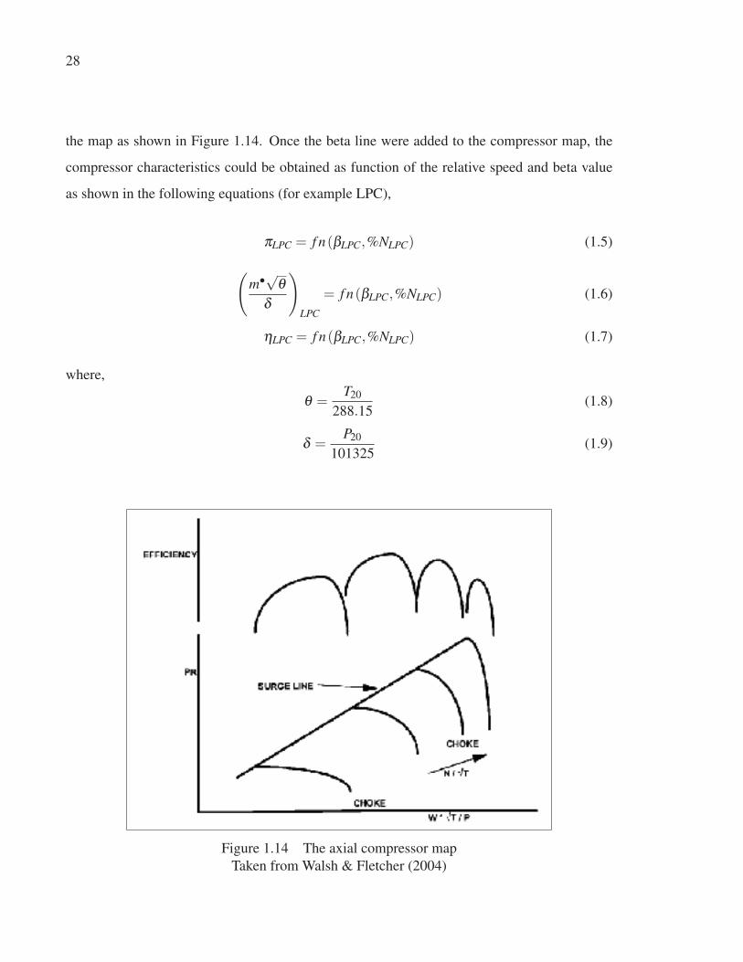
28
the map as shown in Figure 1.14. Once the beta line were added to the compressor map, the
compressor characteristics could be obtained as function of the relative speed and beta value
as shown in the following equations (for example LPC),
πLPC = f n(βLPC,%NLPC) (1.5)
(m•√θ
δ
)LPC
= f n(βLPC,%NLPC) (1.6)
ηLPC = f n(βLPC,%NLPC) (1.7)
where,
θ =T20
288.15(1.8)
δ =P20
101325(1.9)
Figure 1.14 The axial compressor map
Taken from Walsh & Fletcher (2004)
29
Figure 1.15 The compressor map and beta lines
Taken from Walsh & Fletcher (2004)
Once the compressor characteristics are available, all of the compressor exit conditions can be
calculated as follows:
The LPC mathematical model,
P23 = πLPC ∗P22 (1.10)
T23 = T22 ∗⎡⎣1+
πLPC( γa−1
γa )−1
ηLPC
⎤⎦ (1.11)
m•22 =
(m•√θ
δ
)LPC
∗ δ√θ
(1.12)
m•32 = m•
22(1−BLPC) (1.13)
WLPC = m•22 ∗ cpa ∗ (T32 −T22) (1.14)
These equations can be repeated to IPC and HPC.
30
1.3.2.3 Combustor
The purpose of the combustor is to further increase the potential energy content of the working
fluid through combustion of a gaseous fuel and air mixture. The combustor exit parameters
can be calculated based on the combustor inlet conditions, the combustion efficiency, and the
combustor total pressure loss as follows:
m•38 = m•
31 +WF (1.15)
T38 =m•
31 ∗ cpa ∗T31 +WF ∗LHV ∗ηCC
m•38 ∗ cpg
(1.16)
P38 = P31 ∗ (1−ΔPRCC) (1.17)
1.3.2.4 Gas generator turbine
Turbine is used to extract sufficient energy from the hot gases of the combustor to drive the
compressor and other auxiliary power equipment. As with compressors, to calculate the gas
generator turbine exit conditions, it is required to know the turbine inlet conditions and the
turbine characteristics (mass flow rate, pressure ratio, and isentropic efficiency) for a given
spool speed and beta line value (Turbine map). Once the turbine characteristics are available,
all of the turbine exit conditions can be calculated as follows:
The HPT mathematical model,
P415 =P40
πHPT(1.18)
T415 = T40 ∗[
1−ηHPT (1−πHPT
(γg−1
γg
))
](1.19)
m•415 = m•
40 +(1−BHPC)m•26 (1.20)
WHPT = m•40 ∗ cpg ∗ (T40 −T415) (1.21)
These equations can be repeated to IPT.
31
1.3.2.5 Power turbine
Power turbine is used to extract sufficient energy from the hot gases of the combustor to drive
the LPC and external load (generator for power generation application). All of the power
turbine exit conditions can be calculated as follows:
P454 =P44
πLPT(1.22)
T454 = T44 ∗[
1−ηLPT (1−πLPT
(γg−1
γg
))
](1.23)
m•454 = m•
44 +(1−BHPC to PT )m•26 +(1−BIPC to PT )m•
24 (1.24)
WPT = m•44 ∗ cpg ∗ (T44 −T454) (1.25)
1.3.2.6 Exhaust nozzle
The purpose of the exhaust duct in the aero derivative gas turbine engines is typically to direct
the exhaust gases into the atmosphere, which is different from exhaust nozzles in aero gas
turbine engines. There is no work done of the flow through the exhaust duct. In addition,
the performance of the exhaust nozzle is defined by the pressure recovery from the engine to
the free stream (exhaust nozzle pressure loses). The exhaust nozzle output parameters can be
calculated as shown in the following equations,
T5 = T52 (1.26)
P52 = (1−ΔPRex)∗P5 (1.27)
32
1.3.2.7 Load
The load characteristic is an important piece of the dynamic modelling because the load applied
to the power turbine affects on steady state and transient performance parameters such as surge
margins, spool speeds, and turbine inlet temperature.
1.3.2.8 Engine dynamics
The engine is said to be in a steady-state, when the internal state of the GTE (P, T, N) reaches
a thermodynamic equilibrium. That means, there is no change in their values and the work
generated by the turbine equal to the required work for the engine compressor and external
load on the same shaft. However, if there is an imbalance of power on the same engine shaft
required to acceleration or deceleration operation, the engine is said to be in a transient state.
There are three main phenomena particular to the transient performance of the turbine engine:
shaft dynamics caused by the inertial effect, pressure dynamics caused by the mass storage
effect, and temperature dynamics caused by the energy storage. Shaft dynamics represents
the simplest and the most important dynamic behavior of the GTE. Based on the principle of
Newtonian mechanics, the shaft dynamic equations for the three spool ADGTE (SGT-A650)
are represented by the following equations,
dNLPC
dt=
3600
4∗π2 ∗NLPC ∗ JLPC[WLPT −WLPC −Load] (1.28)
dNIPC
dt=
3600
4∗π2 ∗NIPC ∗ JIPC[WIPT −WIPC] (1.29)
dNHPC
dt=
3600
4∗π2 ∗NHPC ∗ JHPC[WHPT −WHPC] (1.30)
To capture the pressure and thermal dynamics, a control volume is inserted between each pair
of engine modules to allow for the mass and energy storage, which gives rise in pressure
and temperature dynamics. Figure 1.16 shows a control volume with temperature, pressure,
and density are assumed to be constant throughout the control volume and equal to the outlet
33
values. In addition, m is the mass of air/gas trapped inside the volume, and V is the volume
of the element. To derive the pressure dynamic equation, assuming that the air/gas within the
control volume behaves like a perfect gas (equation (1.31)). So, the rate of change of mass
inside the volume is proportional to rate of change of pressure and temperature as shown in
equation (1.32).
PV = mRT (1.31)
P•2 =
mRV
∗T •2 +
RT2
V∗m• (1.32)
In equation (1.32), the temperature derivative can be neglected in comparison to the mass
derivative term (Jaw & Mattingly, 2009). So that, equation (1.32) can be written as,
P•2 =
RT2
V∗m• (1.33)
From the law of conservation of mass, the rate of change of mass m trapped inside the control
volume is determined by the difference between the amount of mass flow rate entering and
leaving the element as shown in equation (1.34),
m• = m•1 −m•
2 (1.34)
Substituting by equation (1.34) into equation (1.33). Then, the rate of change of pressure within
the control volume is given by,
P•2 =
RT2
V∗ [m•
1 −m•2] (1.35)
With respect to the temperature dynamics, based on the conservation of energy law, the rate of
change of the internal energy of the control volume can be given by,
U• = m•1cpT1 −m•
2cpT1 +Enet (1.36)
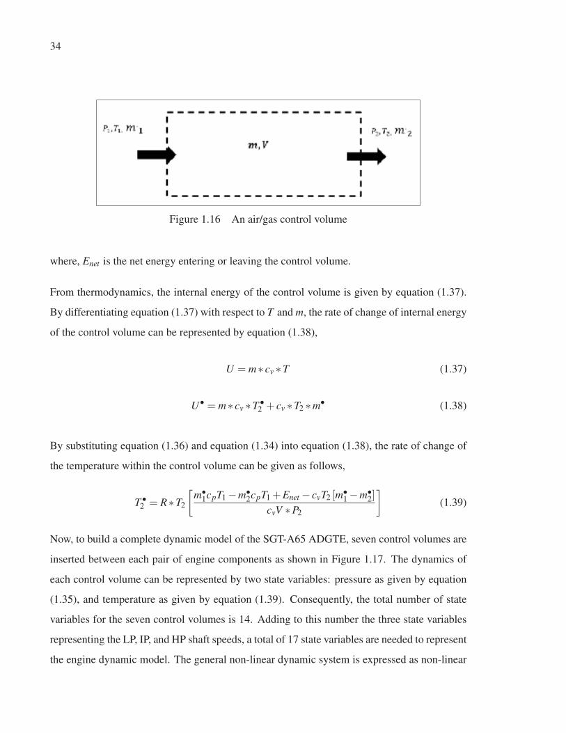
34
Figure 1.16 An air/gas control volume
where, Enet is the net energy entering or leaving the control volume.
From thermodynamics, the internal energy of the control volume is given by equation (1.37).
By differentiating equation (1.37) with respect to T and m, the rate of change of internal energy
of the control volume can be represented by equation (1.38),
U = m∗ cv ∗T (1.37)
U• = m∗ cv ∗T •2 + cv ∗T2 ∗m• (1.38)
By substituting equation (1.36) and equation (1.34) into equation (1.38), the rate of change of
the temperature within the control volume can be given as follows,
T •2 = R∗T2
[m•
1cpT1 −m•2cpT1 +Enet − cvT2 [m•
1 −m•2]
cvV ∗P2
](1.39)
Now, to build a complete dynamic model of the SGT-A65 ADGTE, seven control volumes are
inserted between each pair of engine components as shown in Figure 1.17. The dynamics of
each control volume can be represented by two state variables: pressure as given by equation
(1.35), and temperature as given by equation (1.39). Consequently, the total number of state
variables for the seven control volumes is 14. Adding to this number the three state variables
representing the LP, IP, and HP shaft speeds, a total of 17 state variables are needed to represent
the engine dynamic model. The general non-linear dynamic system is expressed as non-linear
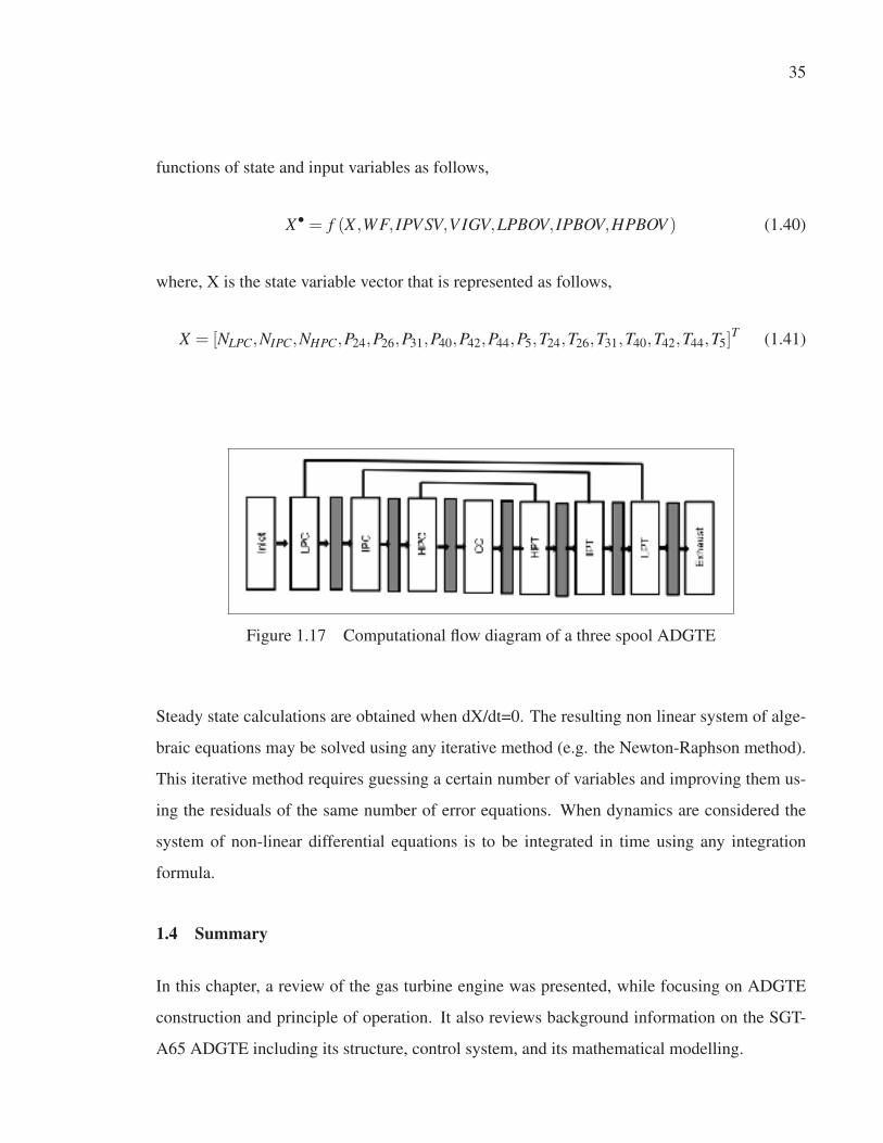
35
functions of state and input variables as follows,
X• = f (X ,WF, IPV SV,V IGV,LPBOV, IPBOV,HPBOV ) (1.40)
where, X is the state variable vector that is represented as follows,
X = [NLPC,NIPC,NHPC,P24,P26,P31,P40,P42,P44,P5,T24,T26,T31,T40,T42,T44,T5]T (1.41)
Figure 1.17 Computational flow diagram of a three spool ADGTE
Steady state calculations are obtained when dX/dt=0. The resulting non linear system of alge-
braic equations may be solved using any iterative method (e.g. the Newton-Raphson method).
This iterative method requires guessing a certain number of variables and improving them us-
ing the residuals of the same number of error equations. When dynamics are considered the
system of non-linear differential equations is to be integrated in time using any integration
formula.
1.4 Summary
In this chapter, a review of the gas turbine engine was presented, while focusing on ADGTE
construction and principle of operation. It also reviews background information on the SGT-
A65 ADGTE including its structure, control system, and its mathematical modelling.

36
As can be seen, the complete thermodynamic dynamic model of the SGT-A65 ADGTE is very
complicated and requires an iterative solution that occurs at the expense of computation time.
The purpose of this chapter was to foster a basic understanding of a gas turbine as relevant
to this project, and highlight the reason why it is imperative to use a data-driven model of
the SGT-A65 three spool engine for real-time model-based applications instead of the highly
complicated thermodynamic model.
CHAPTER 2
LITERATURE REVIEW
2.1 Introduction
Modelling and simulation of gas turbines plays a key role in manufacturing and improving
performance of gas turbine engines. In recent years, the importance of ADGTEs in the energy
industry has sparked a great interest among manufacturers to improve the performance and
increase the reliability of the engine, which in turn requires an accurate and real time model
to simulate the engine dynamics during the full operating range. This chapter presents a com-
prehensive overview of the most significant studies in the field of modelling, simulation and
control of ADGTEs. It covers both physics based and data driven based models of ADGTEs.
This chapter also presents a survey of the historical development of GTE control systems. Be-
sides, it emphasizes on the most significant publications in the field of advanced controller
design for industrial GTEs . The concluding remarks from the literature review are presented
at the end of this chapter.
2.2 Modelling and simulation of gas turbine engines
Before making a gas turbine engine model, some basic factors should be carefully considered
such as modelling objectives, GTE type, GTE configuration, and modelling methods. These
factors are considered among the most important criteria at the beginning of the modelling
process. There are different objectives for making a GTE model. A GTE can be modelled
for condition monitoring, fault detection and diagnosis, sensor validation, system identifica-
tion, design optimization and improvement of control systems. Thus, a clear statement of the
modelling objectives is necessary to make a successful GTE model (Asgari & Chen, 2015). A
real-time simulation can be used as a powerful tool in developing, testing and tuning control
devices of GTEs (Camporeale et al., 2006). In addition, it can be used to simulate critical
transients scenarios that should be avoided on the actual plant due to risk of damage.
38
The first step of modelling a GTE is defining the type and configuration of the engine which
is to be modelled. It is necessary to get enough information about the input/output param-
eters, engine specifications, and engine configuration. GTEs can be classified according to
their applications to aero GTEs and stationary GTEs. More details about the GTEs types and
configuration will be mentioned in the next chapter.
Throughout the years many methods were developed to simulate GTE dynamic response. In-
vestigating GTE dynamic response began around the early 1950s, and ranged from a simple
linear models (Otto & Taylor III, 1951; Rowen, 1983) to a real time high fidelity non-linear
models (Camporeale et al., 2006; Gazzetta Junior et al., 2017; Montazeri-Gh et al., 2018;
Petkovic et al., 2019).
GTE modelling methods can be categorized into two main groups including physics based
modelling methods (white-box models) and data driven based modelling methods (black-box
models). In some cases, the expression of gray-box model may also be used as a combination
of the last two methods (Asgari et al., 2014). The next subsections present a comprehensive
overview of the most significant studies in white and black box modelling, including their
characteristics, benefits, and limitations.
2.2.1 Physics based modelling of GTEs
Physics based models are based on first principles such as the law of physics, chemistry, etc
(Nguyen, 2000). This approach has been widely used over many years in order to model gas
turbine engines (Ballin, 1988; Duyar et al., 1995; Bettocchi et al., 1996; Saleh, 2017; Tahan
et al., 2017; Petkovic et al., 2019). However, this approach can only be used when there
is enough information about the physics of the system. In addition, a white box model has
traditionally a high number of non linear equations requiring iterative solutions which occur at
the expense of computation time. The computation time challenge of the physics based model
is a big problem for real time modelling, especially when the system to model consists of a
high number of subsystems as in case of three spool GTEs.
39
Gas turbine physics model consists of both an off-design steady-state model and an off-design
dynamic model. Both types of models are derived based on the first principles of physics
(Jaw & Mattingly, 2009). When the internal state of an engine reaches a thermodynamic
equilibrium, that is, there is no change in the values of state variables, the engine is said to be
in a steady state. However, dynamic or transient model determines the time history of engine
state and path followed by the engine from its existing steady state to the new steady-state
condition because of a disturbance in load demand and/or ambient conditions (Sanghi et al.,
2000). Off-design conditions refer to the state where the GTE is operated in conditions which
are beyond the standard designed condition.
All off-design steady-state calculations depend on satisfying the essential conditions of match-
ing of mass flow across two adjacent stations, rotational speed and power balance between the
compressor, turbine, and load on the same shaft. These are often referred to as component
matching calculations (H.I.H. Saravanamuttoo, 2017). To generate an off-design steady-state
model of the GTE, a set of non-linear thermodynamic algebraic equations are solved iteratively
to ensure that there is a match between each engine components. This iteration can be achieved
either via serial nested loops method, or via a matrix method. For both iteration methods, there
are several matching guesses, and an equal number of matching constraints (matching of mass
flow and work). During iteration the matching guesses are continually updated until the match-
ing constraints are satisfied. For serial nested loops method, the matching guesses parameters
and matching constraints are paired and solved in a nested sequence. Whereby for each pass
through higher loop, each loop within it is repeated until convergence. This technique is often
easier to understand physically, and to implement via personal computer programs. However,
this technique becomes computationally inefficient for more than five nested loops (Muir et al.,
1989; Kyprianidis & Kalfas, 2008; H.I.H. Saravanamuttoo, 2017; Yazar et al., 2017). On the
other hand, in the matrix iteration method, the overall interaction is recognized and the con-
straint equations are set and solved simultaneously. This requires a numerical method, such
as Newton-Raphson, which is utilizing partial derivatives. These partial derivatives represent
the effect of changing each matching guess individually on the errors in all the matching con-
40
straints (Walsh & Fletcher, 2004). The matrix iteration method is now more common and a
powerful method for simulation of advanced GTEs (Gaudet, 2008; Gu et al., 2016; Zhou et al.,
2020). However, this numerical solver has shown some limits when applied to real time sim-
ulation due to the need of calculation of the Jacobian matrix in every iteration. To save some
time, the Broyden method may be used to replace the Newton method derivative by a finite dif-
ference. So, the Jacobian matrix will be calculated only at the first iteration and to do rank-one
updates at other iterations. Even though, the total number of system evaluations is generally
much lower and the total computation speed faster than for the Newton-Raphson, the rate of
convergence is smaller than for the Newton–Raphson method with a Jacobian determined by
difference quotients (Krummrein et al., 2018).
As stated above, steady-state response relied on the fact that compatibility of flow and compat-
ibility of work must be satisfied at all time. However, during transient operations, a mismatch
of work between the compressor, turbine, and load is required to allow the engine to accelerate
or decelerate. Therefore the assumption of compatibility of work and flow is no longer valid
during transient operations (Fawke & Saravanamuttoo, 1971). GTEs have three main types of
dynamics which should be considered during dynamics modelling: shaft dynamics, pressure
dynamics, and temperature dynamics. To model these dynamics phenomenons, there are two
methods for treating flow and work imbalance during dynamic modelling: Constant mass flow
iterative (CMF) method (Kong et al., 1999; Thirunavukarasu, 2013; Forhad & Bloomberg,
2015), and Inter-component volume (ICV) method (Camporeale et al., 2006; Petkovic et al.,
2019). In the CMF method, shaft dynamics can be modelled only. The CMF approach assumed
that the mass flow of the air (or gas) entering an engine component must equal the mass flow
leaving the same component (Zhu & Saravanamuttoo, 1992). As stated, the basic assumption
in the CMF approach is that flow compatibility is maintained at all times. So that, to predict
the engine behavior during a transient, the calculation proceeds as follows: An initial guess is
made for certain engine parameters. After that, a single run through the engine calculations
is made. The error in mass flows are then noted and progressively minimized by improving
the initial guess through a numerical method such as the Newton–Raphson method. So, many
41
iterations are performed until the error value reached to the required degree of accuracy. Once
flow compatibility was achieved, the work imbalance on the engine shaft may be used to rep-
resent the shaft dynamics as shown in equation (2.1), and an integration method may be used
to predict the shaft speed. On the other hand, to represent the pressure and thermal dynamics
of the GTE, the ICV method can be used. The ICV method always assumes flow mismatch
and work mismatch between engine components during transient performance. This is done by
inserting a control volume between engine components and applying the conservation of mass
and energy laws as shown in equations (2.2) and (2.3). A comprehensive expatiation of these
equations were presented in the previous chapter. Moreover, the ICV method is considered as a
popular and accurate choice for transient performance prediction. In (Tsoutsanis et al., 2013),
hybrid CMF-ICV approaches were used to model the dynamic performance of an industrial
GTE. The employment of both the ICV and CMF methods improves the computational time
and the prediction accuracy of the engine model.
The differential equations that define the engine dynamics ( equations (2.1) to 2.3)) may be
solved by employing integration methods such as the Euler method (Gaudet, 2008; Wang,
2016), Runge-Kutta method (Kim et al., 2001; Petkovic et al., 2019), etc. However, these
integration methods have shown some limits when applied to real time simulation due to con-
straints on step time. The step time should be no greater than one-tenth the magnitude of the
smallest time constant the user wants to observe. Stamatis et al. (2001) stated that, the fre-
quency range over which the GTE model is representative can vary between 1 Hz for models
with only shaft dynamics to 30-50 Hz with pressure dynamics included, and so integration time
step can vary between 50 ms for the lower order models to 1 ms for high order models. There-
fore, a larger step time can be used in the CMF method, which decreases the computation time.
On the other hand, in the ICV method, a shorter step time is necessary for correct prediction
of the transient, which increases the computation time. In order to obtain a real time execution
of the model, the integration of this set of differential equations, at each step time, must be
completed by the computer within a time shorter than the assumed step time.
dNdt
=3600
4∗π2 ∗N ∗ J[WT −WC −Load] (2.1)
42
dPdt
=R∗T
V∗ [m•
in −m•out ] (2.2)
dTout
dt= R∗Tout
[m•
incpT1 −m•outcpTin +Enet − cvTout [m•
in −m•out ]
cvV ∗Pout
](2.3)
As can be seen, the physics based model of the GTE consists of a mixed set of non-linear al-
gebraic equations and ordinary differential equations. In order to obtain a real time execution
of this model, all the calculations of the iterative procedure and solution of differential equa-
tions must be completed by the computer within a time shorter than the assumed time step.
Real-time simulation can be used as a powerful tool in developing, testing and tuning con-
trol devices of gas turbines. Moreover, it can be possible to simulate critical manoeuvres that
should be avoided on the actual engine due to risk of damage. However, a problem that arises
when using physical performance model for real time simulation is that the computational time
varies at each time step due to the necessary iterations. Furthermore, the iterative method
produces noise on the output parameters due to solutions at each time step are falling at ran-
dom places within the permitted tolerance band. This noise may prevent assessment of system
stability, due to the perturbations produced (Walsh & Fletcher, 2004). The fastest achievable
sampling rate depends on the complexity of the engine, the degree of detail of the modelling,
and on the available computing power. Therefore, to enable calculation in real time, software
and hardware approaches have been proposed by many researchers.
For software approaches, in order to reduce the computational time, techniques based on the
simplification of the detailed thermal model (physics based model), the utilization of more
efficient iteration techniques, and the utilization of more efficient integration techniques may
be used. The simplification of the physics model includes the usage of the reduced-order
thermal model (Crainic et al., 1997; Rosini et al., 2019). However, this leads to a decreasing of
model accuracy. It is also possible to simplify the detailed engine model by linearizing the non-
linear model around selected operating points (Rowen, 1983; Montazeri-Gh & Abyaneh, 2017;
Chen et al., 2019). However, the linearized models should be used only in the neighbourhood
of the working point about which the linearization has been carried out. If simplifications to
the non-linear model can’t be made easily then one may have to resort to efficient iteration
43
and numerical methods. The most effective way to keep optimizing the execution time of a
simulation is to limit the maximum number of iterations the solver takes through the simulation
logic (Lietzau & Kreiner, 2001; Fuksman & Sirica, 2012). Another extremely powerful feature
of the iteration method which improves both convergence success rate and time until reach the
solution is the selection of the starting point close to the final solution (Gazzetta Junior et al.,
2017). Also, the usage of the Broyden method to update the Jacobian matrix in the Newton-
Raphson method may reduce the model computation time (Krummrein et al., 2018). With
respect to the integration methods, Stamatis et al. (2001) developed a real time engine model
of two spool GTE. They carried out a comparison between explicit and implicit integration
methods in order to study its impact on the execution time. They concluded that no obvious
advantage is noticed between explicit and implicit integration. However, for smaller number
of fixed iterations implicit integration seems to be faster than explicit integration, while the
opposite is valid when increasing the number of fixed iterations. Moreover, one iteration of the
code costs about 0.25-0.3 ms using implicit or explicit Euler integration method in Pentium
450 MHz and 2-3 ms in a Pentium 90 MHz. In another effort, Lin et al. (1999) presented a
hybrid integration method for real time simulation of single spool GTE. The hybrid integration
method allowed to enlarge the time step to 20 ms and the integration still remains stable. In
some cases, the most desirable approach to achieve real-time simulation is speeding up the
calculations though expensive and faster hardware (Sanjawadmath & Suresh, 2017) or parallel
processing. Finally, the implementation of real-time models must also balance the constraints
of cost and execution time.
As can be seen, the computation time challenge is a big problem for real time modelling of
the physics based model, especially when the system to model consists of a high number of
subsystems as in our case: (SGT-A65) is a three spool ADGTE, the execution time study for
Siemens’s high fidelity thermodynamic model resulted in exceeding the sampling time (10
ms) in real time simulation for ramp and step load change using Speedgoat performance real
time target machine with Intel Quad-Core i7 3770K @ 3.5 GHz CPU, 4096 MB of RAM. An
alternative to white box models is given by data-driven based models.
44
2.2.2 Data driven based modelling of GTEs
Data-driven based model (or black box model) is one of the modelling approaches which can
be used when no or little information is available about the physics of the system. In this case,
a data driven model can disclose the relations between system variables using the obtained
operational input and output data from the system. Artificial neural network is one of the
most significant methods in data-driven based modelling (Asgari et al., 2013). It presents
high computation speed, which allows for real time applications. It is a fast-growing method,
which has been used in different fields of industry in recent years. It is also being heavily
used in machine learning and artificial intelligence applications. The main idea behind ANN
is to create a model based on a human brain in order to solve complex scientific and industrial
problems in a variety of areas.
Linear NN were first proposed by Widrow and Hoff in the 1960s with the name ADALINE
(Widrow & Hoff, 1960), and have been used as the typical NN architecture until the cre-
ation of the back propagation algorithm (BP), which provides a tool for training non-linear
multi-layer perceptron neural networks (MLP) in the late 1980s Rumelhart et al. (1985). Cy-
benko(Cybenko, 1989) proved that a neural network with one hidden layer of sigmoid or hy-
perbolic tangent units and an output layer of linear units is capable of approximating any con-
tinuous function. The network is described by the magnitude of the weights and biases and
is determined by training the network with the operational or simulated data. In the area of
modelling and simulation of industrial gas turbine engines, there are many sources in the liter-
ature. Asgari et al. (Asgari et al., 2013) presented a general overview of essential basic criteria
that need to be considered for making a satisfactory model and control system of a gas turbine
engine. It covers both white-box and black box modelling approaches.
Neural networks can be classified into two main categories: static and dynamic neural net-
works(Ibrahem et al., 2019). Static neural networks are the simplest neural networks, and are
characterized by memoryless non linear equations, which means that there are no feedback
elements and no delays in the network input. Therefore, the output parameters from the static
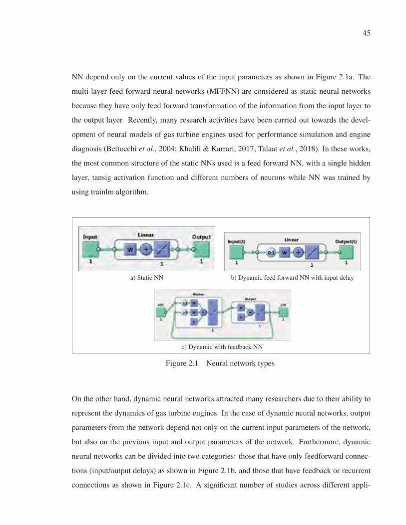
45
NN depend only on the current values of the input parameters as shown in Figure 2.1a. The
multi layer feed forward neural networks (MFFNN) are considered as static neural networks
because they have only feed forward transformation of the information from the input layer to
the output layer. Recently, many research activities have been carried out towards the devel-
opment of neural models of gas turbine engines used for performance simulation and engine
diagnosis (Bettocchi et al., 2004; Khalili & Karrari, 2017; Talaat et al., 2018). In these works,
the most common structure of the static NNs used is a feed forward NN, with a single hidden
layer, tansig activation function and different numbers of neurons while NN was trained by
using trainlm algorithm.
a) Static NN b) Dynamic feed forward NN with input delay
c) Dynamic with feedback NN
Figure 2.1 Neural network types
On the other hand, dynamic neural networks attracted many researchers due to their ability to
represent the dynamics of gas turbine engines. In the case of dynamic neural networks, output
parameters from the network depend not only on the current input parameters of the network,
but also on the previous input and output parameters of the network. Furthermore, dynamic
neural networks can be divided into two categories: those that have only feedforward connec-
tions (input/output delays) as shown in Figure 2.1b, and those that have feedback or recurrent
connections as shown in Figure 2.1c. A significant number of studies across different appli-
46
cations have stated the advantages of dynamic NNs by introducing different methodologies
(Tayarani-Bathaie et al., 2014; Yu & Shu, 2017). Among the existing dynamic NN modelling
methods, the non-linear autoregressive network with exogenous inputs (NARX) modelling ap-
proach is considered one of the most popular. It has been used in the modelling of gas turbine
engines by several researchers Mehrpanahi et al. (2018); Salehi & Montazeri-Gh (2018); Tarik
et al. (2017); Bahlawan et al. (2017).
NARX is a recurrent dynamic network with feedback connections enclosing several layers of
the network. Note that static neural networks (feed forward) have no feedback elements and
contain no delays; the output depends only on the current value of the input to the network.
However, in dynamic neural networks, the output depends on the current and previous inputs
and outputs of the network. In addition, dynamic networks can be divided into two categories,
those that only have a tapped delay line on the input but no feedback connections and those
that have feedback or recurrent connections and tapped delay line on the input (such as NARX
networks) (Ibrahem et al., 2019). NARX model is based on the linear ARX model, which
is commonly used in time-series modelling, and is used in many applications such as multi
step ahead prediction and modelling of non-linear dynamic systems. Equation(2.4) defines a
NARX model and represents the relation between the model output and its input parameters
(Beale et al., 2015),
y(t) = f (y(t −1), · · · ,y(t −ny),u(t −nk), · · · ,u(t −nk −nu +1)) (2.4)
where, ny and nu are the lags of the output and input of the system respectively. nk is the system
input-output delay and f is a non-linear function.
As can be seen, the major challenge to the application of ANNs is to find the best structure
of the network which can represent the system. In this regard, usage of single neural model
may not be able to provide accurate prediction when it operates outside the field in which it
was trained. Besides, gas turbine engines operate in non-stationary operation conditions which
may cause unseen scenarios in the observed data. As a result, this increases the complexity of
47
the modelling operation since the NN needs to be trained with a data as large enough to cover
the entire operation conditions. This in turn increases the training time and the possibility of
network over-fitting. To address this problem, we consider to train multiple ANNs in parallel
to fit the data instead of a single model. This leads to an ensemble of neural network models.
Ensemble learning approach refers to a set of models working in parallel on tasks such as
classification or regression, and they are combined together in some way to obtain the final
output (de Sousa et al., 2012). The ensemble development process can be divided into three
main steps. The first step is ensemble generation, which refers to generation of ensemble base
models. The second step is ensemble pruning, which consists of selecting a subset of the best
models from the original set of models based on generalization error. Finally, ensemble inte-
gration, a strategy to combine the base models is defined. For regression problems, ensemble
integration is done using a linear combination of the base models outputs (de Sousa et al.,
2012),
fen(x) =K
∑i=1
[wi(x)∗ fi(x)] (2.5)
where, wi(x) denotes the weight for the ith model, K is the number of models in the ensemble,
fi(x) denotes the output of the ith model corresponding to input x and fen(x) represents the
ensemble output. Diversity is a very important key in the ensemble generation. If all ensem-
ble members provide the same output, there is nothing to be gained from their combination
(Zhang & Ma, 2012). Therefore, the ensemble members should be different from each other
while each must maintain acceptable accuracy level (Amozegar & Khorasani, 2016). Two dif-
ferent methodologies can be considered for creating diversity among ensemble members. The
first method is heterogeneous ensemble in which ensemble members have different architec-
tures( such as number of neurons, training algorithm ). The second method is homogeneous
ensemble in which ensemble members have the same architectures but trained with different
data sets (Brown et al., 2005). The integration of a set of learned models to improve accuracy
and generalization is another important step in the ensemble generation. Ensemble integration
approaches can be divided into two categories,constant and non-constant weighting functions
(Merz & Pazzani, 1999). Examples of the constant weight approach are basic ensemble method
48
(BEM), generalized ensemble method (GEM), linear regression (LR) and median method. For
the second category, the weights vary according to performance of each ensemble member
such as dynamic weighting (DW), dynamic weight with selection (DWS)(Rooney & Patterson,
2007) and dynamic and on-line ensemble regression (DOER)(Soares & Araújo, 2015).
In recent years, the ensemble approach attracted many researchers and good results have been
reported (de Sousa et al., 2012; Amozegar & Khorasani, 2016). The advantage of ensembles as
compared to single models has been presented in terms of increase of robustness and general-
ization (Zhang & Ma, 2012). In the area of gas turbine engines, (Wang et al., 2014; Wen et al.,
2019; Lu et al., 2019; Behera et al., 2019; Li et al., 2019) used ensemble learning for tack-
ling the fault detection identification (FDI) problem and prediction of the RUL of gas turbine
engine. (Amozegar & Khorasani, 2016; Xu et al., 2017) developed ensemble of multiple learn-
ers to identify the gas turbine engine dynamics. In this thesis, we will focus on the ensemble
generation for regression.
2.3 Advanced control of gas turbine engine
Control technology has a key role in development and progressing the performance, reliability,
operating life, and safety of modern GTEs. The power output from a GTE is determined by fuel
flow, and the control system must ensure that the desired power output is achieved. However,
the control system must also protect the engine from exceeding any design limits. These limits
include component speeds, temperatures and operating regions which can result in compressor
surge (Razak, 2007). So that, the control system for a typical gas turbine in a power generation
application carries out three primary functions: Engine staring and shut-down sequencing,
Control, and Protection.
The implementation of GTE control systems has changed dramatically over the past half-
century. Since 1950s, the computing section and the fuel metering section of the control system
were incorporated into a hydro-mechanical system in which fuel passing through the unit pro-
vided the necessary hydraulic actuation of a variety of pistons, bellows and levers which me-
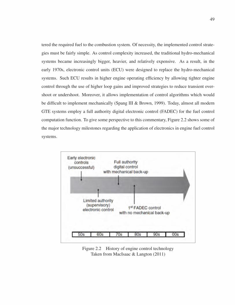
49
tered the required fuel to the combustion system. Of necessity, the implemented control strate-
gies must be fairly simple. As control complexity increased, the traditional hydro-mechanical
systems became increasingly bigger, heavier, and relatively expensive. As a result, in the
early 1970s, electronic control units (ECU) were designed to replace the hydro-mechanical
systems. Such ECU results in higher engine operating efficiency by allowing tighter engine
control through the use of higher loop gains and improved strategies to reduce transient over-
shoot or undershoot. Moreover, it allows implementation of control algorithms which would
be difficult to implement mechanically (Spang III & Brown, 1999). Today, almost all modern
GTE systems employ a full authority digital electronic control (FADEC) for the fuel control
computation function. To give some perspective to this commentary, Figure 2.2 shows some of
the major technology milestones regarding the application of electronics in engine fuel control
systems.
Figure 2.2 History of engine control technology
Taken from MacIsaac & Langton (2011)
50
New designs and operations of modern GTEs are increasingly complex, where several con-
straints and control modes should be satisfied simultaneously to achieve a safe and optimal
performance for the engine. There are several control strategies proposed to deal with these
requirements dating back to 1952. A comprehensive review and analysis on the history of
GTEs control strategies could be found in (Jaw & Mattingly, 2009). The Min–Max control
strategy is commonly used as the control architecture for GTEs to provide desired power, and
prevent the engine from exceeding any safety or operational limits. This strategy is known as
a practical algorithm to satisfy all engine control modes simultaneously without any error and
malfunction. A min-max controller composed of several control loops (steady state loop, max
acceleration loop, max shaft loop speed, max temperature loop, and min deceleration loop),
each of which takes the task of observing a different engine controlling mode. These loops
are in parallel and at any moment, according to a predefined fuel control strategy, one of them
is selected and undertakes the observation (Spang III & Brown, 1999; Montazeri-Gh et al.,
2016; Salehi & Montazeri-GH, 2020). Many studies have done for performance improvement
of the min-max strategy (Chipperfield & Fleming, 1996; Montazeri-Gh & Jafari, 2011; Esfa-
hani & Montazeri, 2016; Jafari & Nikolaidis, 2018). However, in all these studies the final
selection strategy between the transient control loops are kept fixed. Moreover, limit violation
may occur for some variables during transient operation. Recent studies have shown that, there
is no guarantee for min-max algorithm with linear compensator to protect engine limits during
transient state(Imani & Montazeri-Gh, 2017; Montazeri-Gh & Rasti, 2019).
With the desire to have more robustness and flexibility of the next generation of the GTE
control systems to achieve ambitious targets and severe limitations set by governments and or-
ganizations such as reduction of NOx emission, reduction of fuel consumption, and increase of
engine life time, the industry is interested in developing another advanced control strategy that
will satisfy the mentioned requirements. MPC is an advanced model-based controller which
has attracted the attention of researchers in recent years. The application of MPC to control
GTE is introduced by Vroemen and Essen (Vroemen et al., 1999; Van Essen & De Lange,
2001). The philosophy behind the construction of MPC laws is radically different from tra-
51
ditional error-feedback control approaches. Instead of producing a control action in response
to the current and past errors, MPC makes a prediction of future system behavior based on its
open loop model, the current system state, the input trajectory, or a disturbance entering the
system. Then, it selects the best possible input action according to a cost function. To do this it
has to solve an optimization problem, subject to possible constraints. Finally, it applies the first
element of the optimal selected input sequence to the plant. At each time step, this procedure is
repeated, which introduces the so-called receding horizon principle (Richter, 2011). MPC used
in a wide variety of application areas including power plants, chemical industries and etc. The
main reason for this is its constraint handling capacity. Unlike most other traditional control
strategies, constraints on inputs and outputs can be incorporated into the MPC optimization.
Another benefit of MPC is its ability to predict future events as soon as they enter the prediction
horizon. Finally, MPC is an essentially multi-variable control strategy, implying that control
loops do not need to be decoupled, because all interactions between multiple inputs and outputs
are accounted for by the model (Camacho & Alba, 2013).
There are various MPC algorithms only differ among themselves in the onboard model used
to represent the controlled process. If a linear model is used for prediction, The MPC ap-
proaches which use for prediction linear models are usually named linear MPC algorithm
(LMPC) (Mu & Rees, 2004; Ghorbani et al., 2008a; Pandey et al., 2018). However, If a non-
linear model is used for prediction, The MPC approaches which use for prediction non-linear
models are usually named non-linear MPC algorithm (NMPC) (Brunell et al., 2002; Kim et al.,
2013; Pires et al., 2018b). In recent years, there have been extensive interests in the general-
ized predictive control (GPC) algorithm, which is one of the most popular predictive control
algorithms and has been successfully applied in industry, particularly in chemical processes,
power, and gas turbines (Mu & Rees, 2004; Aly & Atia, 2012; Ye et al., 2017). The basic idea
of GPC is to calculate a sequence of future control signals in such a way that it minimizes a
cost function defined over a prediction horizon. The index to be optimized is the expectation
of a quadratic function measuring the distance between the predicted system output and some
predicted reference sequence over the prediction horizon plus a quadratic function measuring
52
the control effort (Camacho & Alba, 2013). Moreover, the GPC is applicable to the systems
with non-minimal phase, unstable systems in open loop, systems with unknown or varying
dead time and systems with unknown order (Pivonka & Nepevny, 2005).
Ghorbani et al. (2008b) used a linear ARX model in a multi-variable MPC strategy for a gas
turbine power plant, and the same authors used the same model type in a constrained MPC
strategy for a heavy-duty gas turbine power plant (Ghorbani et al., 2008a). Mohamed et al.
(2016) presented a strategy for implementing LMPC to a large gas turbine power plant. A
generalized state space model for that engine was used as an onboard model within the LMPC.
Also, Pandey et al. (2018) designed a MIMO linear state-space model to simulate the response
of 5 MW industrial GTE at certain operating condition, then be used to design a LMPC for
this engine. Based on the fact that GTE is inherently non-linear. The inherent non-linearity
together with higher product quality specifications, increasing productivity demands, tighter
environmental regulations, and demanding economical considerations require to operate sys-
tems over a wide range of operating conditions and often near the boundary of the safe region.
Under these conditions linear models are often not sufficient to describe the process dynamics
adequately and non-linear models must be used. This inadequacy of linear models is one of
the motivations for the increasing interest in NMPC.
Pires et al. (2018a) designed a NMPC to reduce the NOx emissions of a single-shaft industrial
GTE. The non-linear dynamic behavior of the engine is modelled using the academic DESTUR
program, a comprehensive first principle computational modelling tool. Four optimization al-
gorithms are used to minimize the objective function, and their performances are compared:
differential evolution, particle swarm, genetic algorithm, and pattern search method. The au-
thors concluded that, the computational effort is higher for the MIMO system. However, The
four algorithms perform well and are viable for the SISO system implementation.
Kim et al. (2013) proposed a NMPC to control the speed and temperature of a 166 MW a
single-shaft heavy-duty gas turbine power plant. A reduced order model with 1 sec sampling
rate is used to simplify calculations. As can be seen, the usage of a non-linear physics based
53
model within the NMPC changes the control problem from a convex quadratic program to
a nonconvex non-linear problem. Furthermore, in this situation, there is no guarantee that
the global optimum can be found especially in real-time control when the optimum has to be
obtained in a prescribed time. Besides, the physics based model should be run many times
faster than real time to allow usage of this model as model based inside the MPC algorithm.
Therefore, a set of efficient approaches that try to avoid the problems associated to nonconvex
optimization has appeared in recent years. One of the simplest ways of dealing with process
non-linearities is to perform successive linearization about a nominal operating point. Every
sampling period an updated linear model is derived from an underlying non-linear model. In
recent years, the successive linearization approach attracted many researchers and good re-
sults have been reported (Van Essen & De Lange, 2001; Mu & Rees, 2004; Niu & Liu, 2008;
Theoklis et al., 2019; Montazeri-Gh & Rasti, 2019). The advantage of using this method over
conventional non-linear design is the avoidance of the problem of local minimums. However,
this could result in a large computational load for MIMO systems. Furthermore, the lineraized
model is only an approximation of the original non-linear one. Therefore, the obtained control
quality may be unsatisfactory for non-linear systems, in particular when the operating point is
changed significantly and fast.
As can be seen, the generation of accurate model which can run many times faster than real
time, is a big challenge in NMPC design. The use of the ANN in NMPC has been recognized as
a effective tool for handling some difficult control process problems, and has recently attracted
a great deal of attention (Rusnak et al., 1996; Sørensen et al., 1999), primarily because ANN
appear to provide a convenient means for modelling complex non-linear processes with good
accuracy and less computational complexity. Two main approaches were used to utilise non-
linear neural model in a predictive control scheme (Aly & Atia, 2012). The first idea is to use
the non-linear optimization to get the optimum control (Lazar & Pastravanu, 2002). The other
is to linearize the non-linear neural model every time step to get the discrete linearized model
(Mu & Rees, 2004; Mu et al., 2005). Pivonka & Nepevny (2005) designed a constrained GPC
based on NN model. Authors stated that the designed controller is adaptive, as it based on NN
54
model which can observe system changes and adapt itself. Rusnak et al. (1996) presented the
GPC algorithm based on ANN plant model. To obtain the step and the free process responses
which are needed in the GPC, the feed-forward ANN model was used to estimate the free
and forced responses. The system free response is obtained instantaneously from ANN model
while forced response is obtained from instantaneous linearization of the ANN model. This
method considered as a trade-off between NMPC and successive linearization approach.
In contrast to LMPC, where convex quadratic programs are mostly solved exactly at each sam-
pling time, NMPC faces an issue: either the non-linear iteration procedure is performed until a
pre-specified convergence criterion is met, or the procedure is stopped prematurely with only
an approximate solution, so that a pre-specified computation time limit can be met. In (Diehl
et al., 2009), the authors gave an overview of Newton type methods for online solution of non-
linear optimal control problems. The two big families of Newton type optimization methods,
SQP and Interior-point methods were presented. The authors concluded that, NMPC results in
improved control performance and allows the direct use of physics based models. However,
the consideration of non-linear models also poses challenging theoretical, computational, and
implementational problems especially for real time applications. Pires et al. (2018b) stated
that, computation of the gradient may not be feasible or cost-effective when using a non-linear
model within NMPC. Therefore, search methods or heuristic methods become attractive. The
maximum number of iteration is an important parameter for theses methods. The control per-
formance could be improved with the increase in the maximum iteration number. However, it
will be computationally expensive.
2.4 Conclusion of literature
This chapter presented a comprehensive overview of the literature in the field of modelling,
simulation, and control of gas turbines. As it can be seen from the literature, there is a great
gain from the research in this field like gas turbine performance evolution and optimization
before and after design and manufacture processes. Therefore, the most relevant scientific
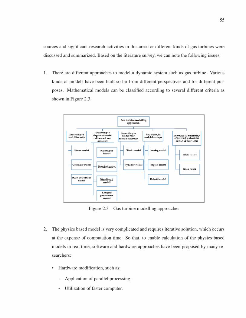
55
sources and significant research activities in this area for different kinds of gas turbines were
discussed and summarized. Based on the literature survey, we can note the following issues:
1. There are different approaches to model a dynamic system such as gas turbine. Various
kinds of models have been built so far from different perspectives and for different pur-
poses. Mathematical models can be classified according to several different criteria as
shown in Figure 2.3.
Figure 2.3 Gas turbine modelling approaches
2. The physics based model is very complicated and requires iterative solution, which occurs
at the expense of computation time. So that, to enable calculation of the physics based
models in real time, software and hardware approaches have been proposed by many re-
searchers:
• Hardware modification, such as:
- Application of parallel processing.
- Utilization of faster computer.
56
• Software modification, such as:
- Utilization of more efficient iteration techniques.
- Utilization of simple models (neglecting the secondary effect parameters).
- Permitting increased off-line calculation, and thus reducing the required on-line
calculations.
3. The computation time challenge is not a big problem for the performance applications.
However, this is not the case for the model-based applications. In the case of model based
application, the physics based model should be accurate. Besides that, it must run many
times faster than real time. An alternative to physics based models is given by data-driven
based models, which can represent dynamics of non-linear systems with good accuracy
and very low computation effort. So that, the data-driven based models are recommended
by many researchers for using in model based applications.
4. Most of static and dynamic ANN research activities on gas turbine engines used a certain
structure of neural networks namely, a feed forward neural network, one hidden layer
with a number of neurons in this layer ranging from nine to twelve, a tansig activation
function in the hidden layer and purelin activation function in the output layer. Finally,
Levenberg-Marquardt algorithm is used as a training algorithm. It is important therefore to
test other combinations, and to perform an extensive performance comparative study using
a combination of different network architectures, training algorithms, activation functions,
system order and different number of neurons. This will be done in this study.
5. In the area of MIMO ANN model of gas turbine engines, the research activities used
mostly one of the following two methods to generate a nonlinear model for the MIMO
engine: Either, by building a neural network model for each output parameter (MISO)
with the same structure for each one of them and trained with the same training algorithm
(Bahlawan et al., 2017), or by building one block neural model to represent the MIMO
system (Tarik et al., 2017; Mehrpanahi et al., 2018; Salehi & Montazeri-Gh, 2018). How-
ever, it is more powerful, as will be shown in this study, to use a different neural network’s
57
structure for each output (MISO). The idea of using different NN structures for different
outputs comes from analysis of the structure of the human brain based on its function.
Human brain consists of many complex biological neural networks; each has to perform a
certain function [talk, walk, breath and so on] as shown in Figure 2.4. The main compo-
nent of these neural networks are neurons. The shape and number of the neurons in each
network depend upon the function of the network. For example, a single sensory neuron
from your fingertip has an axon that extends the length of your arm, while neurons within
the brain may extend only a few millimetres. They also have different shapes depending
on their functions (Khan, 2018). Motor neurons that control muscle contractions have a
cell body on one end, a long axon in the middle and dendrites on the other end. Sensory
neurons have dendrites on both ends, connected by a long axon with a cell body in the
middle. Inter-neurons, or associative neurons, carry information between motor and sen-
sory neurons as shown in Figure 2.5. Based on these facts, to generate a neural network
model for an ADGTE, we propose to build MISO neural network model for each output.
Moreover, the structure of each neural model is different according to the function of the
model (output type).
6. As can be seen, the usage of single neural model may not be able to provide accurate
prediction when it operates outside the field in which it was trained. Besides, gas turbine
engines operate in non-stationary operation conditions, which may cause unseen scenarios
in the observed data. This increases the complexity of the modelling operation since the
NN needs to be trained with a data as large enough to cover the entire operation conditions.
This in turn increases the training time and the possibility of network over-fitting. To
address this problem, we consider to train multiple ANNs in parallel to fit the data instead
of a single model. This leads to an ensemble of neural network models.
7. According to the literature, most works on ensemble approach focus on classification ap-
plications for tackling the FDI problem in gas turbine engines (Wang et al., 2014; Wen
et al., 2019; Lu et al., 2019; Behera et al., 2019; Li et al., 2019). However, little research
has been done on the use of ensemble approach for gas turbine engine real time perfor-
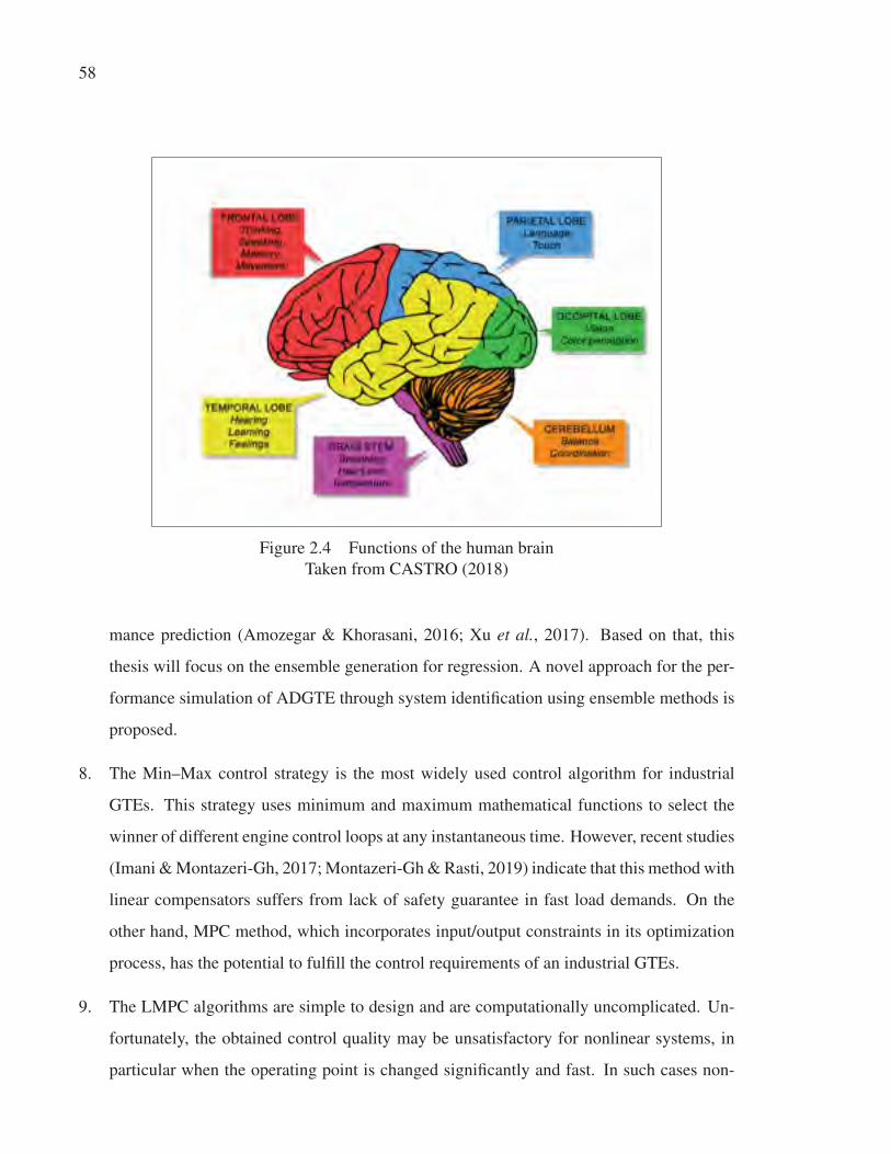
58
Figure 2.4 Functions of the human brain
Taken from CASTRO (2018)
mance prediction (Amozegar & Khorasani, 2016; Xu et al., 2017). Based on that, this
thesis will focus on the ensemble generation for regression. A novel approach for the per-
formance simulation of ADGTE through system identification using ensemble methods is
proposed.
8. The Min–Max control strategy is the most widely used control algorithm for industrial
GTEs. This strategy uses minimum and maximum mathematical functions to select the
winner of different engine control loops at any instantaneous time. However, recent studies
(Imani & Montazeri-Gh, 2017; Montazeri-Gh & Rasti, 2019) indicate that this method with
linear compensators suffers from lack of safety guarantee in fast load demands. On the
other hand, MPC method, which incorporates input/output constraints in its optimization
process, has the potential to fulfill the control requirements of an industrial GTEs.
9. The LMPC algorithms are simple to design and are computationally uncomplicated. Un-
fortunately, the obtained control quality may be unsatisfactory for nonlinear systems, in
particular when the operating point is changed significantly and fast. In such cases non-
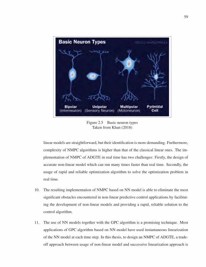
59
Figure 2.5 Basic neuron types
Taken from Khan (2018)
linear models are straightforward, but their identification is more demanding. Furthermore,
complexity of NMPC algorithms is higher than that of the classical linear ones. The im-
plementation of NMPC of ADGTE in real time has two challenges: Firstly, the design of
accurate non-linear model which can run many times faster than real time. Secondly, the
usage of rapid and reliable optimization algorithm to solve the optimization problem in
real time.
10. The resulting implementation of NMPC based on NN model is able to eliminate the most
significant obstacles encountered in non-linear predictive control applications by facilitat-
ing the development of non-linear models and providing a rapid, reliable solution to the
control algorithm.
11. The use of NN models together with the GPC algorithm is a promising technique. Most
applications of GPC algorithm based on NN model have used instantaneous linearization
of the NN model at each time step. In this thesis, to design an NMPC of ADGTE, a trade-
off approach between usage of non-linear model and successive linearization approach is

60
used in order to reduce the computation effort. In addition, in order to solve this prob-
lem, Hildreth’s quadratic programming procedure is utilized which offers simplicity and
reliability in real-time implementation.

CHAPTER 3
NEURAL NETWORKS MODELLING APPROACH
3.1 Introduction
This chapter embodies the real core of this work, which makes it the most extensive chapter
of the thesis. At the next step, ANN model building process including system analysis, data
acquisition and preparation, network architecture, as well as network training and validation
are explained. The last part of the chapter is focused on the generation of ensembles of NN
models.
3.2 Neural network basics
ANN is a non-linear statistical data modelling tool mimicking the neural structure of the human
brain. NNs are composed of simple elements operating in parallel. These elements are inspired
by biological nervous systems. As in nature, the network function is determined largely by the
connections between elements. ANN is trained to perform a particular function by adjusting
the values of the connections (weights) between elements. Each such single element is called
a neuron. Neurons are arranged in different layers including input layer, hidden layer(s) and
output layer. The number of neurons and layers in an ANN model determine the degree of
complexity of the network. Figure 3.1 shows a simple structure of a simple NN with four
inputs, one output and four neurons in two hidden layers.
3.3 ANN modelling approach
There are many challenges in the building operation of neural networks model, which can be
summarized as follows:
• Finding the best neural network type.
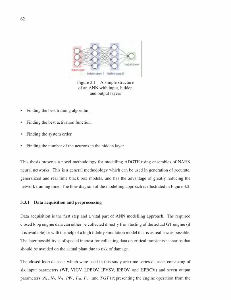
62
Figure 3.1 A simple structure
of an ANN with input, hidden
and output layers
• Finding the best training algorithm.
• Finding the best activation function.
• Finding the system order.
• Finding the number of the neurons in the hidden layer.
This thesis presents a novel methodology for modelling ADGTE using ensembles of NARX
neural networks. This is a general methodology which can be used in generation of accurate,
generalized and real time black box models, and has the advantage of greatly reducing the
network training time. The flow diagram of the modelling approach is illustrated in Figure 3.2.
3.3.1 Data acquisition and preprocessing
Data acquisition is the first step and a vital part of ANN modelling approach. The required
closed loop engine data can either be collected directly from testing of the actual GT engine (if
it is available) or with the help of a high fidelity simulation model that is as realistic as possible.
The later possibility is of special interest for collecting data on critical transients scenarios that
should be avoided on the actual plant due to risk of damage.
The closed loop datasets which were used in this study are time series datasets consisting of
six input parameters (WF, VIGV, LPBOV, IPVSV, IPBOV, and HPBOV) and seven output
parameters (NL, NI , NH , PW , T30, P30, and T GT ) representing the engine operation from the
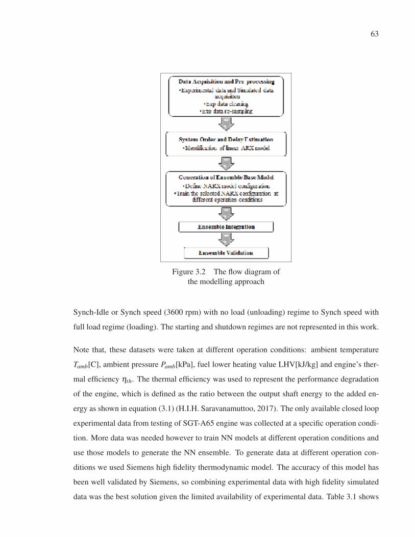
63
Figure 3.2 The flow diagram of
the modelling approach
Synch-Idle or Synch speed (3600 rpm) with no load (unloading) regime to Synch speed with
full load regime (loading). The starting and shutdown regimes are not represented in this work.
Note that, these datasets were taken at different operation conditions: ambient temperature
Tamb[C], ambient pressure Pamb[kPa], fuel lower heating value LHV[kJ/kg] and engine’s ther-
mal efficiency ηth. The thermal efficiency was used to represent the performance degradation
of the engine, which is defined as the ratio between the output shaft energy to the added en-
ergy as shown in equation (3.1) (H.I.H. Saravanamuttoo, 2017). The only available closed loop
experimental data from testing of SGT-A65 engine was collected at a specific operation condi-
tion. More data was needed however to train NN models at different operation conditions and
use those models to generate the NN ensemble. To generate data at different operation con-
ditions we used Siemens high fidelity thermodynamic model. The accuracy of this model has
been well validated by Siemens, so combining experimental data with high fidelity simulated
data was the best solution given the limited availability of experimental data. Table 3.1 shows
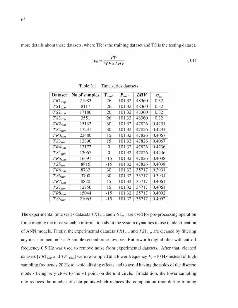
64
more details about these datasets, where TR is the training dataset and TS is the testing dataset.
ηth =PW
WF ∗LHV(3.1)
Table 3.1 Time series datasets
Dataset No of samples TTT amb PPPamb LLLHHHVVV ηηη thT R1exp 21983 26 101.32 48360 0.32
T S1exp 8117 26 101.32 48360 0.32
T S2exp 17186 26 101.32 48360 0.32
T S3exp 3551 26 101.32 48360 0.32
T R2sim 15132 30 101.32 47826 0.4231
T S2sim 17231 30 101.32 47826 0.4231
T R3sim 22480 15 101.32 47826 0.4067
T S3sim 12890 15 101.32 47826 0.4067
T R4sim 13172 0 101.32 47826 0.4236
T S4sim 12067 0 101.32 47826 0.4236
T R5sim 16691 -15 101.32 47826 0.4038
T S5sim 8816 -15 101.32 47826 0.4038
T R6sim 8732 30 101.32 35717 0.3931
T S6sim 3700 30 101.32 35717 0.3931
T R7sim 8820 15 101.32 35717 0.4061
T S7sim 12750 15 101.32 35717 0.4061
T R8sim 15044 -15 101.32 35717 0.4092
T S8sim 21065 -15 101.32 35717 0.4092
The experimental time series datasets T R1exp and T S1exp are used for pre-processing operation
for extracting the most valuable information about the system dynamics to use in identification
of ANN models. Firstly, the experimental datasets T R1exp and T S1exp are cleaned by filtering
any measurement noise. A simple second order low pass Butterworth digital filter with cut-off
frequency 0.5 Hz was used to remove noise from experimental datasets. After that, cleaned
datasets [T R1exp and T S1exp] were re-sampled at a lower frequency Fs =10 Hz instead of high
sampling frequency 20 Hz to avoid aliasing effects and to avoid having the poles of the discrete
models being very close to the +1 point on the unit circle. In addition, the lower sampling
rate reduces the number of data points which reduces the computation time during training
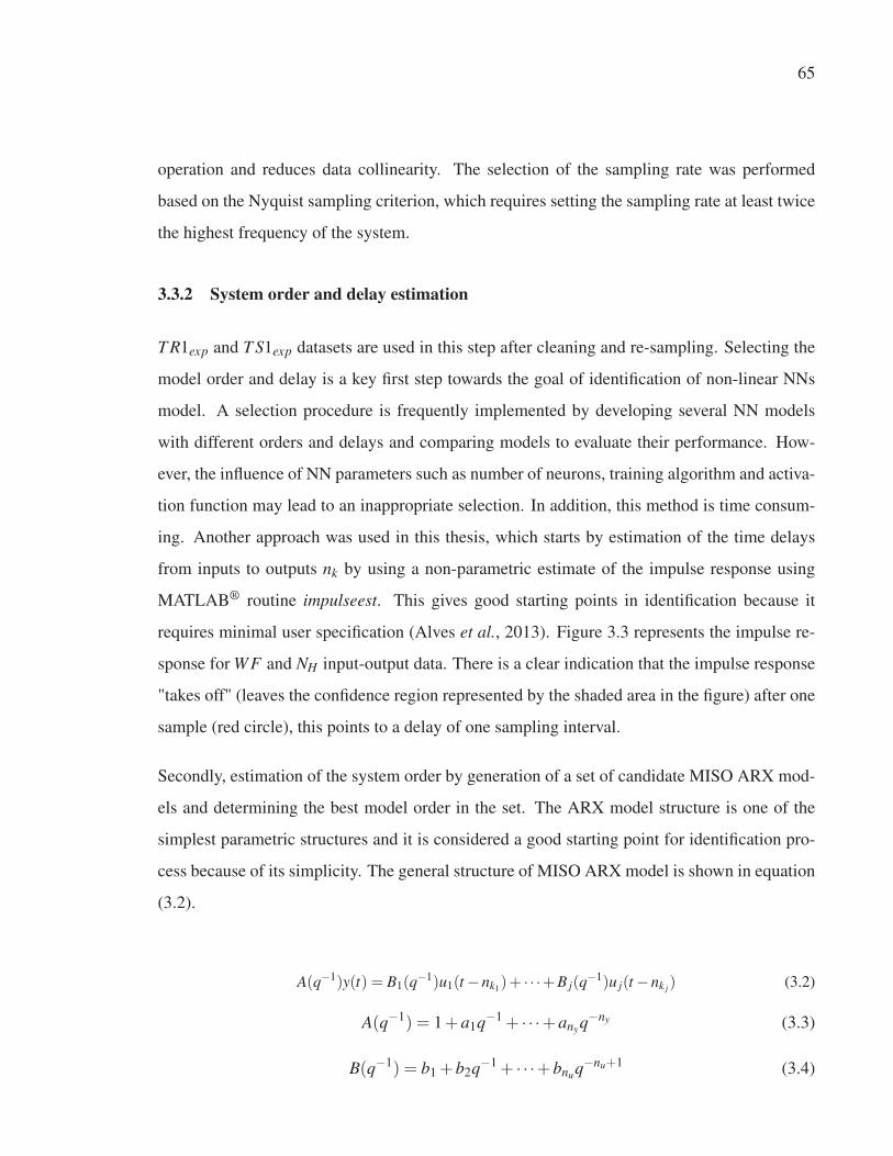
65
operation and reduces data collinearity. The selection of the sampling rate was performed
based on the Nyquist sampling criterion, which requires setting the sampling rate at least twice
the highest frequency of the system.
3.3.2 System order and delay estimation
T R1exp and T S1exp datasets are used in this step after cleaning and re-sampling. Selecting the
model order and delay is a key first step towards the goal of identification of non-linear NNs
model. A selection procedure is frequently implemented by developing several NN models
with different orders and delays and comparing models to evaluate their performance. How-
ever, the influence of NN parameters such as number of neurons, training algorithm and activa-
tion function may lead to an inappropriate selection. In addition, this method is time consum-
ing. Another approach was used in this thesis, which starts by estimation of the time delays
from inputs to outputs nk by using a non-parametric estimate of the impulse response using
MATLAB® routine impulseest. This gives good starting points in identification because it
requires minimal user specification (Alves et al., 2013). Figure 3.3 represents the impulse re-
sponse for WF and NH input-output data. There is a clear indication that the impulse response
"takes off" (leaves the confidence region represented by the shaded area in the figure) after one
sample (red circle), this points to a delay of one sampling interval.
Secondly, estimation of the system order by generation of a set of candidate MISO ARX mod-
els and determining the best model order in the set. The ARX model structure is one of the
simplest parametric structures and it is considered a good starting point for identification pro-
cess because of its simplicity. The general structure of MISO ARX model is shown in equation
(3.2).
A(q−1)y(t) = B1(q−1)u1(t −nk1)+ · · ·+B j(q−1)u j(t −nk j) (3.2)
A(q−1) = 1+a1q−1 + · · ·+anyq−ny (3.3)
B(q−1) = b1 +b2q−1 + · · ·+bnuq−nu+1 (3.4)
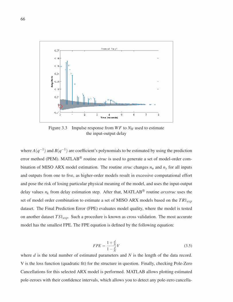
66
Figure 3.3 Impulse response from WF to NH used to estimate
the input-output delay
where A(q−1) and B(q−1) are coefficient’s polynomials to be estimated by using the prediction
error method (PEM). MATLAB® routine struc is used to generate a set of model-order com-
bination of MISO ARX model estimation. The routine struc changes nu and ny for all inputs
and outputs from one to five, as higher-order models result in excessive computational effort
and pose the risk of losing particular physical meaning of the model, and uses the input-output
delay values nk from delay estimation step. After that, MATLAB® routine arxstruc uses the
set of model order combination to estimate a set of MISO ARX models based on the T R1exp
dataset. The Final Prediction Error (FPE) evaluates model quality, where the model is tested
on another dataset T S1exp. Such a procedure is known as cross validation. The most accurate
model has the smallest FPE. The FPE equation is defined by the following equation:
FPE =1+ d
N
1− dN
V (3.5)
where d is the total number of estimated parameters and N is the length of the data record.
V is the loss function (quadratic fit) for the structure in question. Finally, checking Pole-Zero
Cancellations for this selected ARX model is performed. MATLAB allows plotting estimated
pole-zeroes with their confidence intervals, which allows you to detect any pole-zero cancella-
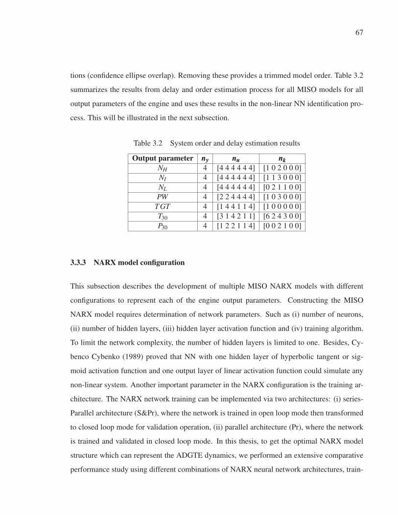
67
tions (confidence ellipse overlap). Removing these provides a trimmed model order. Table 3.2
summarizes the results from delay and order estimation process for all MISO models for all
output parameters of the engine and uses these results in the non-linear NN identification pro-
cess. This will be illustrated in the next subsection.
Table 3.2 System order and delay estimation results
Output parameter nnnyyy nnnuuu nnnkkkNH 4 [4 4 4 4 4 4] [1 0 2 0 0 0]
NI 4 [4 4 4 4 4 4] [1 1 3 0 0 0]
NL 4 [4 4 4 4 4 4] [0 2 1 1 0 0]
PW 4 [2 2 4 4 4 4] [1 0 3 0 0 0]
T GT 4 [1 4 4 1 1 4] [1 0 0 0 0 0]
T30 4 [3 1 4 2 1 1] [6 2 4 3 0 0]
P30 4 [1 2 2 1 1 4] [0 0 2 1 0 0]
3.3.3 NARX model configuration
This subsection describes the development of multiple MISO NARX models with different
configurations to represent each of the engine output parameters. Constructing the MISO
NARX model requires determination of network parameters. Such as (i) number of neurons,
(ii) number of hidden layers, (iii) hidden layer activation function and (iv) training algorithm.
To limit the network complexity, the number of hidden layers is limited to one. Besides, Cy-
benco Cybenko (1989) proved that NN with one hidden layer of hyperbolic tangent or sig-
moid activation function and one output layer of linear activation function could simulate any
non-linear system. Another important parameter in the NARX configuration is the training ar-
chitecture. The NARX network training can be implemented via two architectures: (i) series-
Parallel architecture (S&Pr), where the network is trained in open loop mode then transformed
to closed loop mode for validation operation, (ii) parallel architecture (Pr), where the network
is trained and validated in closed loop mode. In this thesis, to get the optimal NARX model
structure which can represent the ADGTE dynamics, we performed an extensive comparative
performance study using different combinations of NARX neural network architectures, train-
68
ing algorithms and activation functions while using different numbers of neurons. As a result,
a comprehensive computer program was developed in the MATLAB environment. Figure 3.4
shows the flow diagram of the comprehensive computer program for the MISO NARX model
of the ADGTE. This program generates 240 NARX models with different structures by per-
forming the following:
1. Changing of the number of neurons from 1 to 20.
2. Usage of two activation functions logsig and tansig.
3. Usage of three training algorithms trainlm, trainscg and trainbr.
4. Training the network with series-parallel architecture and parallel architecture.
One of the problems that occur during NN training is network over-fitting. The early stopping
and cross validation are the default methods for improving network generalization and reduce
occurrence of over-fitting during the training operation. When the network begins to over-fit
the data, the validation error begins to increase, and after a certain number of iterations, the
training is stopped, and the weights and biases at the minimum validation error is fixed.
In this thesis, the network training parameters are defined as: (i) the mean square error (mse)
performance function which is minimized until it reaches a sufficiently low cut-off value of
(0.01), (ii) the maximum number of training epochs (1000) which represents the number of
times that all the training patterns are presented to the NN and (iii) the maximum number
of validation increase (100) which represents the number of successive epochs in which the
performance function fails to decrease. Training operation was repeated three times for the
same neural network with the same input data set to increase the accuracy of the network.
The T R1exp dataset is partitioned into 80% used for training the network and 20% used for
cross validation. After finishing the network training operation, the T S1exp dataset is used for
testing the network and evaluating its generalization performance. (RMSE) was used for the
evaluation of the network performance in the training and testing operation. It was calculated
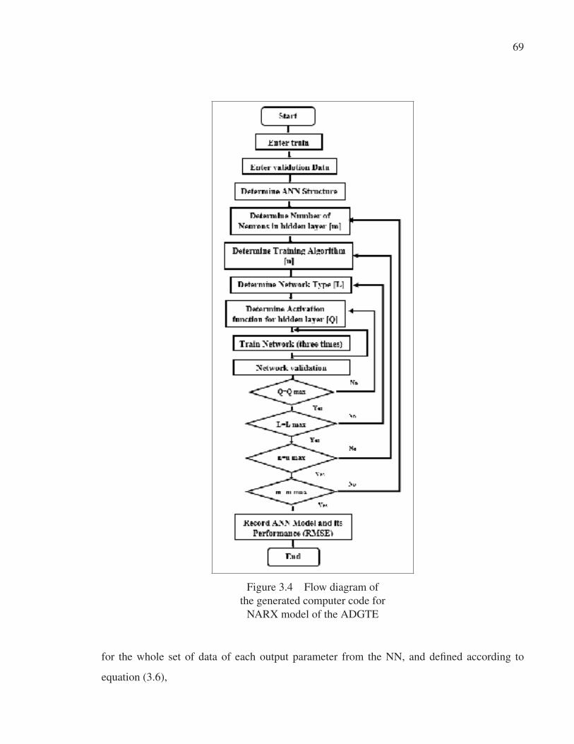
69
Figure 3.4 Flow diagram of
the generated computer code for
NARX model of the ADGTE
for the whole set of data of each output parameter from the NN, and defined according to
equation (3.6),
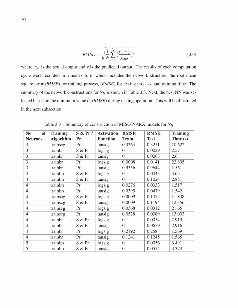
70
RMSE =
√1
N
N
∑i=1
(ym − yymax
)2 (3.6)
where, ym is the actual output and y is the predicted output. The results of each computation
cycle were recorded in a matrix form which includes the network structure, the root mean
square error (RMSE) for training process, (RMSE) for testing process, and training time. The
summary of the network constructions for NH is shown in Table 3.3. Next, the best NN was se-
lected based on the minimum value of (RMSE) during testing operation. This will be illustrated
in the next subsection.
Table 3.3 Summary of construction of MISO-NARX models for NH
No ofNeurons
TrainingAlgorithm
S & Pr /Pr
ActivationFunction
RMSETrain
RMSETest
TrainingTime (s)
3 trainscg Pr tansig 0.3264 0.3251 10.622
3 trainbr S & Pr logsig 0 0.0029 2.57
3 trainbr S & Pr tansig 0 0.0063 2.6
3 trainbr Pr logsig 0.0008 0.0141 22.895
3 trainbr Pr tansig 0.9356 0.9644 1.561
4 trainlm S & Pr logsig 0 0.0043 3.65
4 trainlm S & Pr tansig 0 0.1024 2.851
4 trainlm Pr logsig 0.0276 0.0333 1.517
4 trainlm Pr tansig 0.0395 0.0479 1.542
4 trainscg S & Pr logsig 0.0009 0.1072 11.838
4 trainscg S & Pr tansig 0.0009 0.1194 12.356
4 trainscg Pr logsig 0.0368 0.0312 21.65
4 trainscg Pr tansig 0.0528 0.0389 13.003
4 trainbr S & Pr logsig 0 0.0054 2.919
4 trainbr S & Pr tansig 0 0.0659 2.916
4 trainbr Pr logsig 0.2192 0.258 1.569
4 trainbr Pr tansig 0.1241 0.1245 1.565
5 trainlm S & Pr logsig 0 0.0056 3.491
5 trainlm S & Pr tansig 0 0.0554 3.373
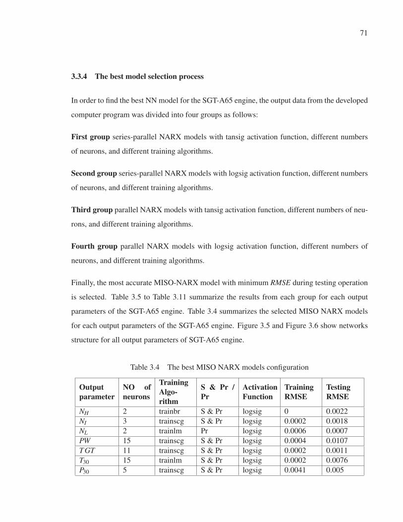
71
3.3.4 The best model selection process
In order to find the best NN model for the SGT-A65 engine, the output data from the developed
computer program was divided into four groups as follows:
First group series-parallel NARX models with tansig activation function, different numbers
of neurons, and different training algorithms.
Second group series-parallel NARX models with logsig activation function, different numbers
of neurons, and different training algorithms.
Third group parallel NARX models with tansig activation function, different numbers of neu-
rons, and different training algorithms.
Fourth group parallel NARX models with logsig activation function, different numbers of
neurons, and different training algorithms.
Finally, the most accurate MISO-NARX model with minimum RMSE during testing operation
is selected. Table 3.5 to Table 3.11 summarize the results from each group for each output
parameters of the SGT-A65 engine. Table 3.4 summarizes the selected MISO NARX models
for each output parameters of the SGT-A65 engine. Figure 3.5 and Figure 3.6 show networks
structure for all output parameters of SGT-A65 engine.
Table 3.4 The best MISO NARX models configuration
Outputparameter
NO ofneurons
TrainingAlgo-rithm
S & Pr /Pr
ActivationFunction
TrainingRMSE
TestingRMSE
NH 2 trainbr S & Pr logsig 0 0.0022
NI 3 trainscg S & Pr logsig 0.0002 0.0018
NL 2 trainlm Pr logsig 0.0006 0.0007
PW 15 trainscg S & Pr logsig 0.0004 0.0107
T GT 11 trainscg S & Pr logsig 0.0002 0.0011
T30 15 trainlm S & Pr logsig 0.0002 0.0076
P30 5 trainscg S & Pr logsig 0.0041 0.005
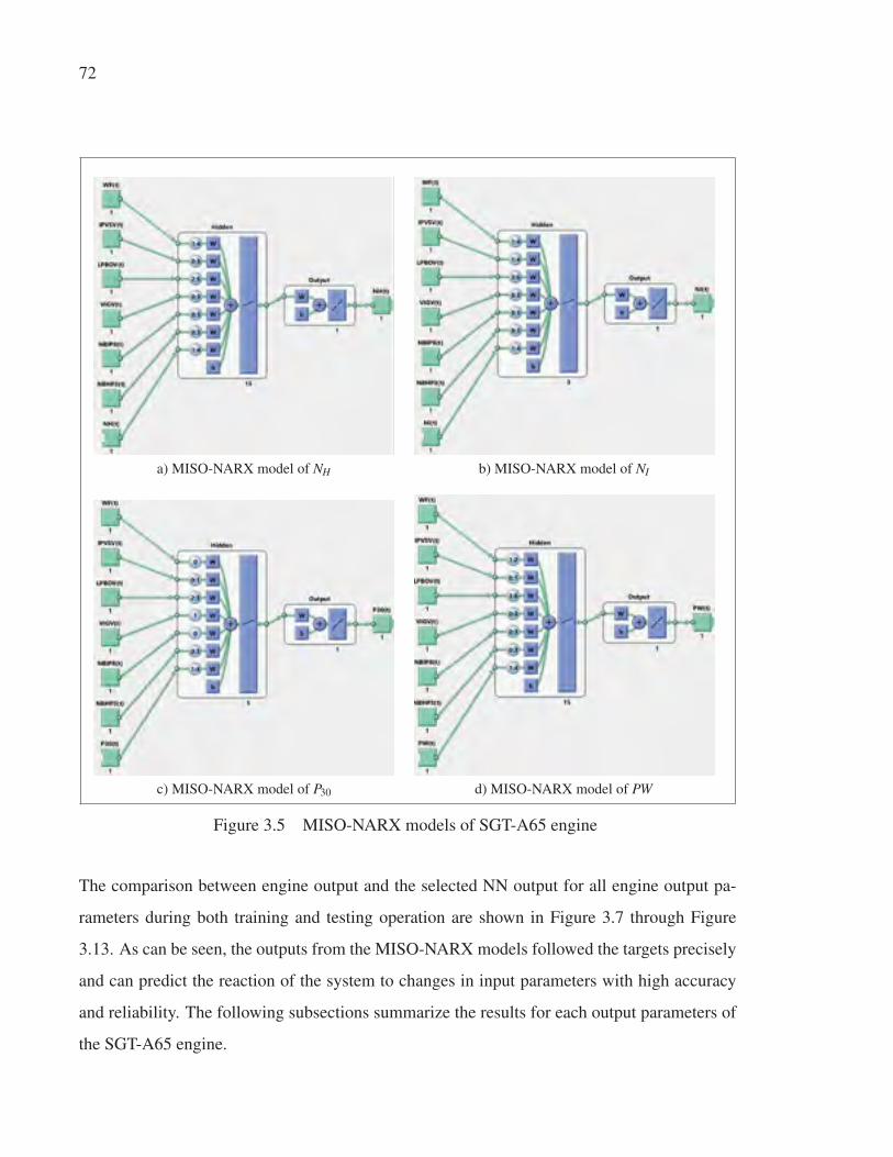
72
a) MISO-NARX model of NH b) MISO-NARX model of NI
c) MISO-NARX model of P30 d) MISO-NARX model of PW
Figure 3.5 MISO-NARX models of SGT-A65 engine
The comparison between engine output and the selected NN output for all engine output pa-
rameters during both training and testing operation are shown in Figure 3.7 through Figure
3.13. As can be seen, the outputs from the MISO-NARX models followed the targets precisely
and can predict the reaction of the system to changes in input parameters with high accuracy
and reliability. The following subsections summarize the results for each output parameters of
the SGT-A65 engine.
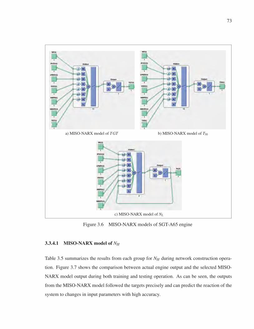
73
a) MISO-NARX model of T GT b) MISO-NARX model of T30
c) MISO-NARX model of NL
Figure 3.6 MISO-NARX models of SGT-A65 engine
3.3.4.1 MISO-NARX model of NH
Table 3.5 summarizes the results from each group for NH during network construction opera-
tion. Figure 3.7 shows the comparison between actual engine output and the selected MISO-
NARX model output during both training and testing operation. As can be seen, the outputs
from the MISO-NARX model followed the targets precisely and can predict the reaction of the
system to changes in input parameters with high accuracy.
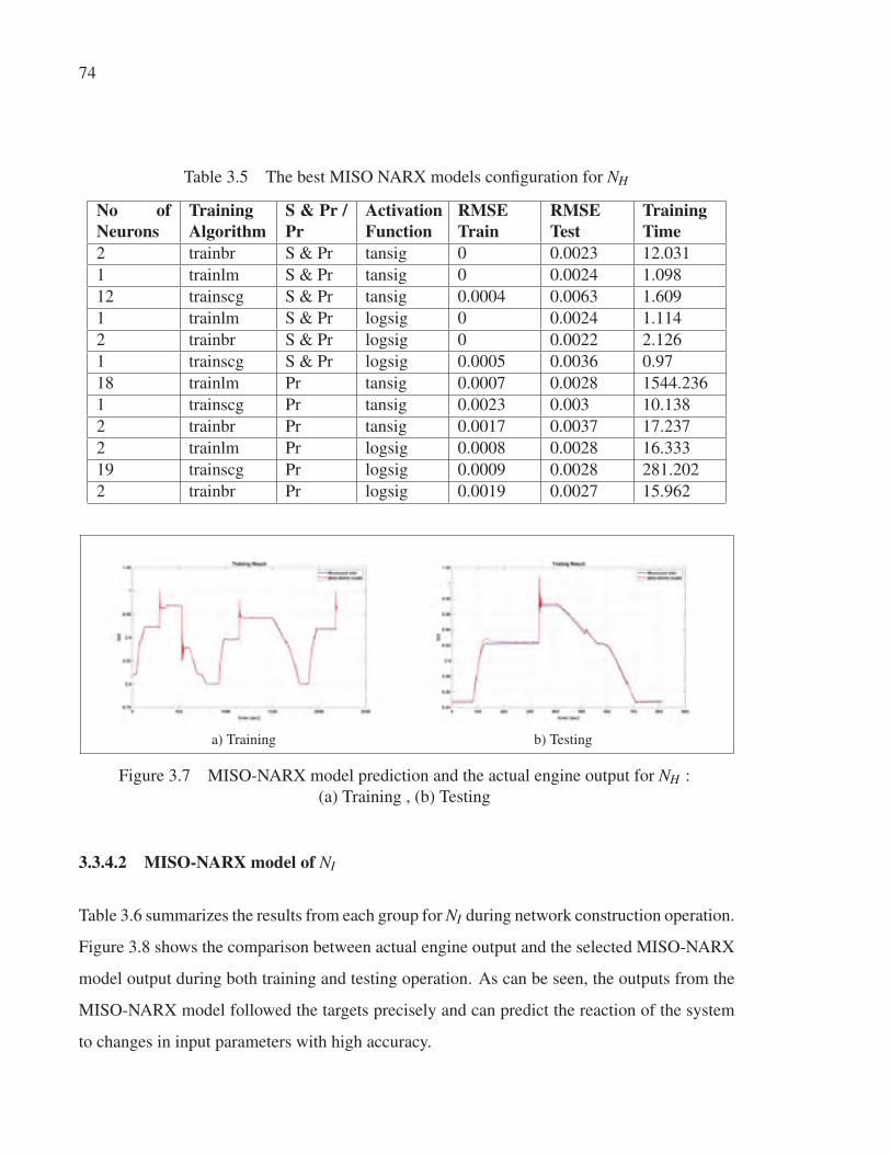
74
Table 3.5 The best MISO NARX models configuration for NH
No ofNeurons
TrainingAlgorithm
S & Pr /Pr
ActivationFunction
RMSETrain
RMSETest
TrainingTime
2 trainbr S & Pr tansig 0 0.0023 12.031
1 trainlm S & Pr tansig 0 0.0024 1.098
12 trainscg S & Pr tansig 0.0004 0.0063 1.609
1 trainlm S & Pr logsig 0 0.0024 1.114
2 trainbr S & Pr logsig 0 0.0022 2.126
1 trainscg S & Pr logsig 0.0005 0.0036 0.97
18 trainlm Pr tansig 0.0007 0.0028 1544.236
1 trainscg Pr tansig 0.0023 0.003 10.138
2 trainbr Pr tansig 0.0017 0.0037 17.237
2 trainlm Pr logsig 0.0008 0.0028 16.333
19 trainscg Pr logsig 0.0009 0.0028 281.202
2 trainbr Pr logsig 0.0019 0.0027 15.962
a) Training b) Testing
Figure 3.7 MISO-NARX model prediction and the actual engine output for NH :
(a) Training , (b) Testing
3.3.4.2 MISO-NARX model of NI
Table 3.6 summarizes the results from each group for NI during network construction operation.
Figure 3.8 shows the comparison between actual engine output and the selected MISO-NARX
model output during both training and testing operation. As can be seen, the outputs from the
MISO-NARX model followed the targets precisely and can predict the reaction of the system
to changes in input parameters with high accuracy.
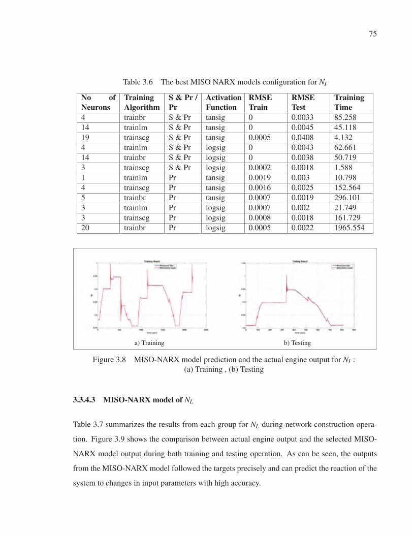
75
Table 3.6 The best MISO NARX models configuration for NI
No ofNeurons
TrainingAlgorithm
S & Pr /Pr
ActivationFunction
RMSETrain
RMSETest
TrainingTime
4 trainbr S & Pr tansig 0 0.0033 85.258
14 trainlm S & Pr tansig 0 0.0045 45.118
19 trainscg S & Pr tansig 0.0005 0.0408 4.132
4 trainlm S & Pr logsig 0 0.0043 62.661
14 trainbr S & Pr logsig 0 0.0038 50.719
3 trainscg S & Pr logsig 0.0002 0.0018 1.588
1 trainlm Pr tansig 0.0019 0.003 10.798
4 trainscg Pr tansig 0.0016 0.0025 152.564
5 trainbr Pr tansig 0.0007 0.0019 296.101
3 trainlm Pr logsig 0.0007 0.002 21.749
3 trainscg Pr logsig 0.0008 0.0018 161.729
20 trainbr Pr logsig 0.0005 0.0022 1965.554
a) Training b) Testing
Figure 3.8 MISO-NARX model prediction and the actual engine output for NI :
(a) Training , (b) Testing
3.3.4.3 MISO-NARX model of NL
Table 3.7 summarizes the results from each group for NL during network construction opera-
tion. Figure 3.9 shows the comparison between actual engine output and the selected MISO-
NARX model output during both training and testing operation. As can be seen, the outputs
from the MISO-NARX model followed the targets precisely and can predict the reaction of the
system to changes in input parameters with high accuracy.
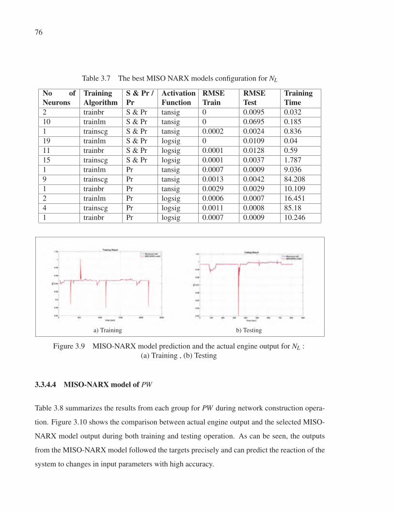
76
Table 3.7 The best MISO NARX models configuration for NL
No ofNeurons
TrainingAlgorithm
S & Pr /Pr
ActivationFunction
RMSETrain
RMSETest
TrainingTime
2 trainbr S & Pr tansig 0 0.0095 0.032
10 trainlm S & Pr tansig 0 0.0695 0.185
1 trainscg S & Pr tansig 0.0002 0.0024 0.836
19 trainlm S & Pr logsig 0 0.0109 0.04
11 trainbr S & Pr logsig 0.0001 0.0128 0.59
15 trainscg S & Pr logsig 0.0001 0.0037 1.787
1 trainlm Pr tansig 0.0007 0.0009 9.036
9 trainscg Pr tansig 0.0013 0.0042 84.208
1 trainbr Pr tansig 0.0029 0.0029 10.109
2 trainlm Pr logsig 0.0006 0.0007 16.451
4 trainscg Pr logsig 0.0011 0.0008 85.18
1 trainbr Pr logsig 0.0007 0.0009 10.246
a) Training b) Testing
Figure 3.9 MISO-NARX model prediction and the actual engine output for NL :
(a) Training , (b) Testing
3.3.4.4 MISO-NARX model of PW
Table 3.8 summarizes the results from each group for PW during network construction opera-
tion. Figure 3.10 shows the comparison between actual engine output and the selected MISO-
NARX model output during both training and testing operation. As can be seen, the outputs
from the MISO-NARX model followed the targets precisely and can predict the reaction of the
system to changes in input parameters with high accuracy.
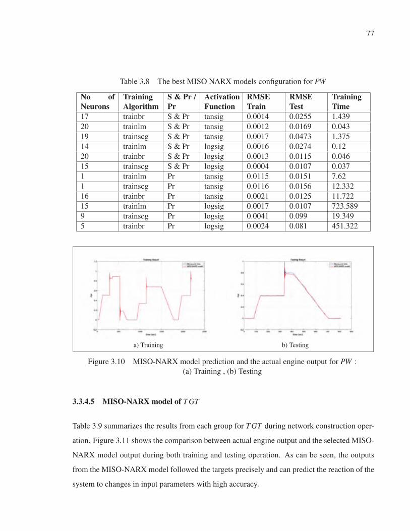
77
Table 3.8 The best MISO NARX models configuration for PW
No ofNeurons
TrainingAlgorithm
S & Pr /Pr
ActivationFunction
RMSETrain
RMSETest
TrainingTime
17 trainbr S & Pr tansig 0.0014 0.0255 1.439
20 trainlm S & Pr tansig 0.0012 0.0169 0.043
19 trainscg S & Pr tansig 0.0017 0.0473 1.375
14 trainlm S & Pr logsig 0.0016 0.0274 0.12
20 trainbr S & Pr logsig 0.0013 0.0115 0.046
15 trainscg S & Pr logsig 0.0004 0.0107 0.037
1 trainlm Pr tansig 0.0115 0.0151 7.62
1 trainscg Pr tansig 0.0116 0.0156 12.332
16 trainbr Pr tansig 0.0021 0.0125 11.722
15 trainlm Pr logsig 0.0017 0.0107 723.589
9 trainscg Pr logsig 0.0041 0.099 19.349
5 trainbr Pr logsig 0.0024 0.081 451.322
a) Training b) Testing
Figure 3.10 MISO-NARX model prediction and the actual engine output for PW :
(a) Training , (b) Testing
3.3.4.5 MISO-NARX model of T GT
Table 3.9 summarizes the results from each group for T GT during network construction oper-
ation. Figure 3.11 shows the comparison between actual engine output and the selected MISO-
NARX model output during both training and testing operation. As can be seen, the outputs
from the MISO-NARX model followed the targets precisely and can predict the reaction of the
system to changes in input parameters with high accuracy.
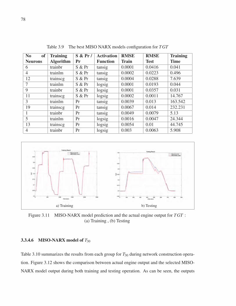
78
Table 3.9 The best MISO NARX models configuration for T GT
No ofNeurons
TrainingAlgorithm
S & Pr /Pr
ActivationFunction
RMSETrain
RMSETest
TrainingTime
6 trainbr S & Pr tansig 0.0001 0.0416 0.041
4 trainlm S & Pr tansig 0.0002 0.0223 0.496
12 trainscg S & Pr tansig 0.0004 0.0288 7.639
7 trainlm S & Pr logsig 0.0001 0.0193 0.044
9 trainbr S & Pr logsig 0.0001 0.0357 0.031
11 trainscg S & Pr logsig 0.0002 0.0011 14.767
3 trainlm Pr tansig 0.0039 0.013 163.542
19 trainscg Pr tansig 0.0067 0.014 232.231
1 trainbr Pr tansig 0.0049 0.0079 5.13
5 trainlm Pr logsig 0.0016 0.0047 24.344
13 trainscg Pr logsig 0.0054 0.01 44.745
4 trainbr Pr logsig 0.003 0.0063 5.908
a) Training b) Testing
Figure 3.11 MISO-NARX model prediction and the actual engine output for T GT :
(a) Training , (b) Testing
3.3.4.6 MISO-NARX model of T30
Table 3.10 summarizes the results from each group for T30 during network construction opera-
tion. Figure 3.12 shows the comparison between actual engine output and the selected MISO-
NARX model output during both training and testing operation. As can be seen, the outputs
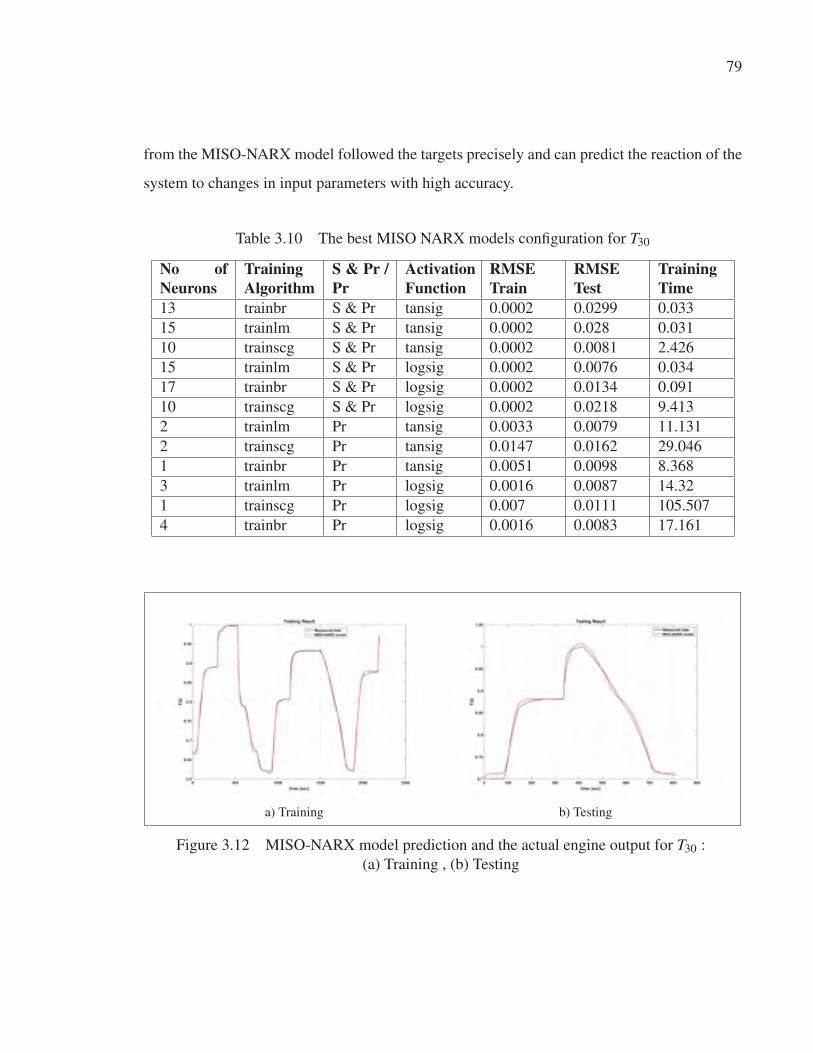
79
from the MISO-NARX model followed the targets precisely and can predict the reaction of the
system to changes in input parameters with high accuracy.
Table 3.10 The best MISO NARX models configuration for T30
No ofNeurons
TrainingAlgorithm
S & Pr /Pr
ActivationFunction
RMSETrain
RMSETest
TrainingTime
13 trainbr S & Pr tansig 0.0002 0.0299 0.033
15 trainlm S & Pr tansig 0.0002 0.028 0.031
10 trainscg S & Pr tansig 0.0002 0.0081 2.426
15 trainlm S & Pr logsig 0.0002 0.0076 0.034
17 trainbr S & Pr logsig 0.0002 0.0134 0.091
10 trainscg S & Pr logsig 0.0002 0.0218 9.413
2 trainlm Pr tansig 0.0033 0.0079 11.131
2 trainscg Pr tansig 0.0147 0.0162 29.046
1 trainbr Pr tansig 0.0051 0.0098 8.368
3 trainlm Pr logsig 0.0016 0.0087 14.32
1 trainscg Pr logsig 0.007 0.0111 105.507
4 trainbr Pr logsig 0.0016 0.0083 17.161
a) Training b) Testing
Figure 3.12 MISO-NARX model prediction and the actual engine output for T30 :
(a) Training , (b) Testing
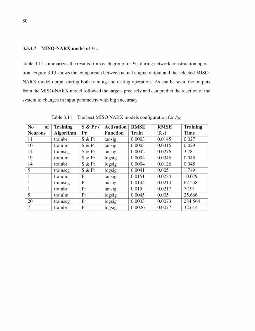
80
3.3.4.7 MISO-NARX model of P30
Table 3.11 summarizes the results from each group for P30 during network construction opera-
tion. Figure 3.13 shows the comparison between actual engine output and the selected MISO-
NARX model output during both training and testing operation. As can be seen, the outputs
from the MISO-NARX model followed the targets precisely and can predict the reaction of the
system to changes in input parameters with high accuracy.
Table 3.11 The best MISO NARX models configuration for P30
No ofNeurons
TrainingAlgorithm
S & Pr /Pr
ActivationFunction
RMSETrain
RMSETest
TrainingTime
11 trainbr S & Pr tansig 0.0003 0.0145 0.027
10 trainlm S & Pr tansig 0.0003 0.0316 0.029
14 trainscg S & Pr tansig 0.0042 0.0276 3.78
19 trainlm S & Pr logsig 0.0004 0.0346 0.045
14 trainbr S & Pr logsig 0.0004 0.0126 0.045
5 trainscg S & Pr logsig 0.0041 0.005 1.749
1 trainlm Pr tansig 0.0151 0.0224 10.079
1 trainscg Pr tansig 0.0144 0.0214 67.258
1 trainbr Pr tansig 0.015 0.0217 7.191
5 trainlm Pr logsig 0.0045 0.005 25.666
20 trainscg Pr logsig 0.0033 0.0073 284.564
7 trainbr Pr logsig 0.0026 0.0077 32.614
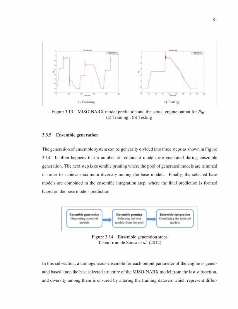
81
a) Training b) Testing
Figure 3.13 MISO-NARX model prediction and the actual engine output for P30 :
(a) Training , (b) Testing
3.3.5 Ensemble generation
The generation of ensemble system can be generally divided into three steps as shown in Figure
3.14. It often happens that a number of redundant models are generated during ensemble
generation. The next step is ensemble pruning where the pool of generated models are trimmed
in order to achieve maximum diversity among the base models. Finally, the selected base
models are combined in the ensemble integration step, where the final prediction is formed
based on the base models prediction.
Figure 3.14 Ensemble generation steps
Taken from de Sousa et al. (2012)
In this subsection, a homogeneous ensemble for each output parameter of the engine is gener-
ated based upon the best selected structure of the MISO-NARX model from the last subsection,
and diversity among them is ensured by altering the training datasets which represent differ-
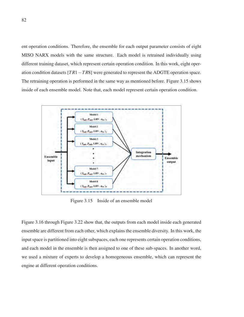
82
ent operation conditions. Therefore, the ensemble for each output parameter consists of eight
MISO NARX models with the same structure. Each model is retrained individually using
different training dataset, which represent certain operation condition. In this work, eight oper-
ation condition datasets [T R1−T R8] were generated to represent the ADGTE operation space.
The retraining operation is performed in the same way as mentioned before. Figure 3.15 shows
inside of each ensemble model. Note that, each model represent certain operation condition.
Figure 3.15 Inside of an ensemble model
Figure 3.16 through Figure 3.22 show that, the outputs from each model inside each generated
ensemble are different from each other, which explains the ensemble diversity. In this work, the
input space is partitioned into eight subspaces, each one represents certain operation conditions,
and each model in the ensemble is then assigned to one of these sub-spaces. In another word,
we used a mixture of experts to develop a homogeneous ensemble, which can represent the
engine at different operation conditions.
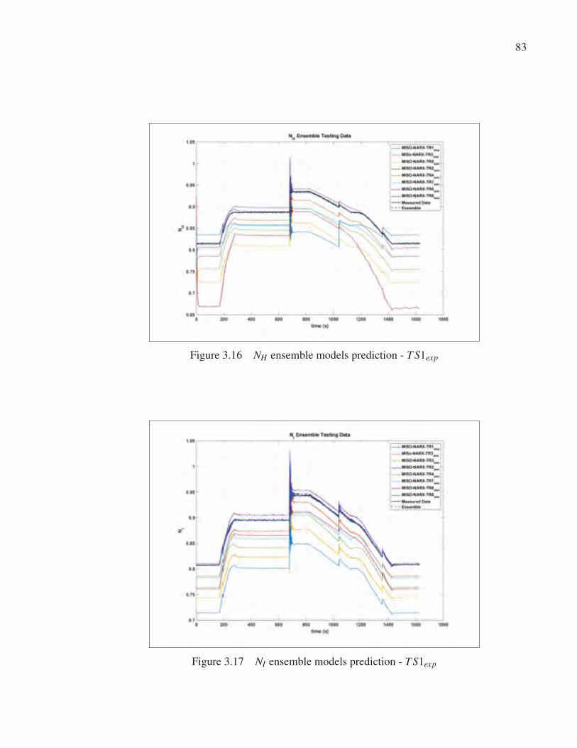
83
Figure 3.16 NH ensemble models prediction - T S1exp
Figure 3.17 NI ensemble models prediction - T S1exp
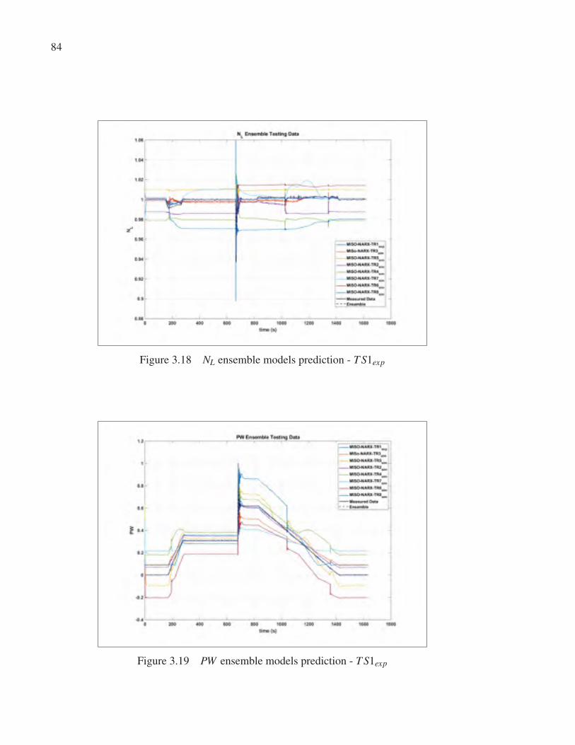
84
Figure 3.18 NL ensemble models prediction - T S1exp
Figure 3.19 PW ensemble models prediction - T S1exp
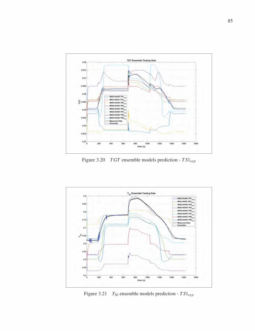
85
Figure 3.20 T GT ensemble models prediction - T S1exp
Figure 3.21 T30 ensemble models prediction - T S1exp
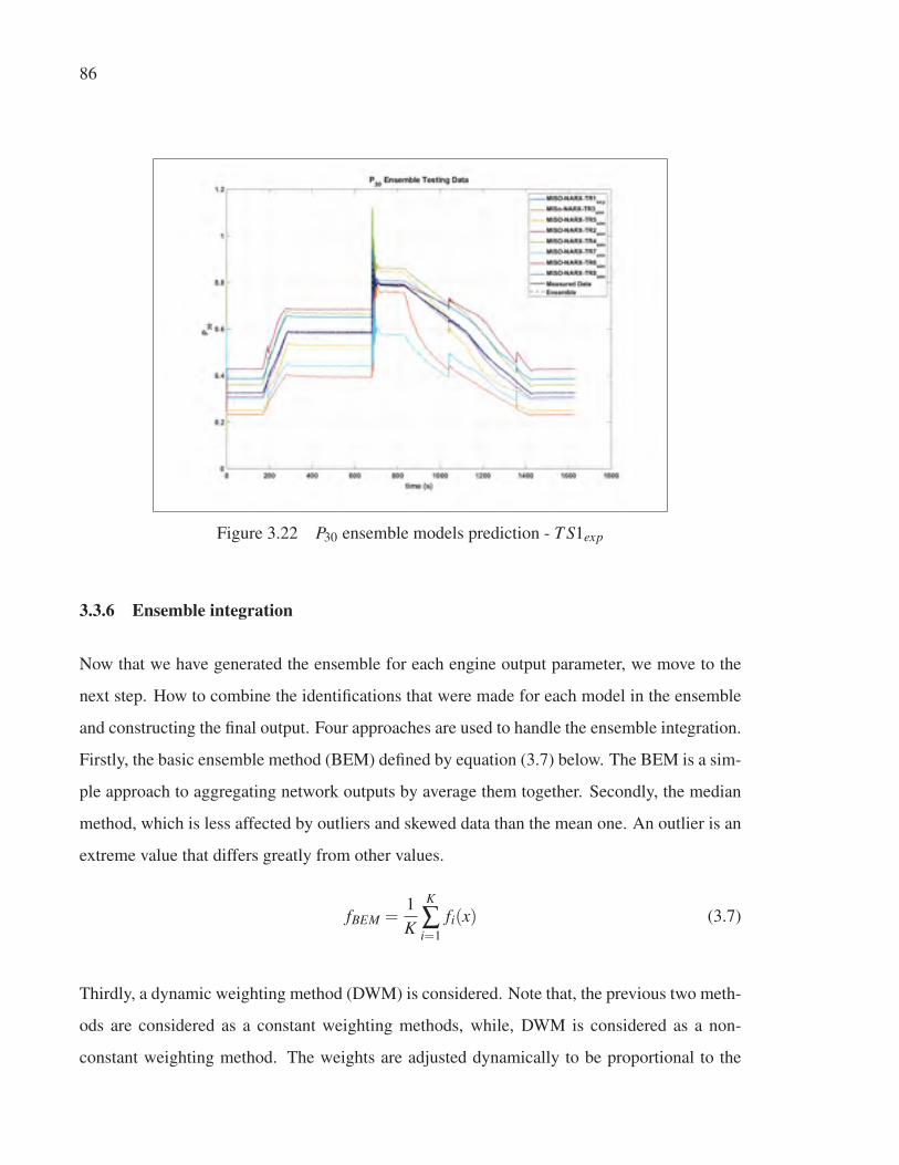
86
Figure 3.22 P30 ensemble models prediction - T S1exp
3.3.6 Ensemble integration
Now that we have generated the ensemble for each engine output parameter, we move to the
next step. How to combine the identifications that were made for each model in the ensemble
and constructing the final output. Four approaches are used to handle the ensemble integration.
Firstly, the basic ensemble method (BEM) defined by equation (3.7) below. The BEM is a sim-
ple approach to aggregating network outputs by average them together. Secondly, the median
method, which is less affected by outliers and skewed data than the mean one. An outlier is an
extreme value that differs greatly from other values.
fBEM =1
K
K
∑i=1
fi(x) (3.7)
Thirdly, a dynamic weighting method (DWM) is considered. Note that, the previous two meth-
ods are considered as a constant weighting methods, while, DWM is considered as a non-
constant weighting method. The weights are adjusted dynamically to be proportional to the
87
performance of ensemble members (MISO NARX models), a greater weight will be assigned
to the ensemble member with better performance. Finally, the proposed HDWM is performed
as follows:
1. Calculation of the performance of each ensemble member as described in equation (3.8),
ei = (ym − yi
ymax)2 (3.8)
2. Calculation of the median value of the models’ errors
MED = median(e1e2 · · ·eK) (3.9)
3. The weight of each model fi is calculated according to its error as described in Eqn. (3.10),
which calculate the weights in such a way: the model i with error ei around the median
value MED receives a weight close to 1. While, models with ei lower than MED have their
weights exponentially increased, and models with ei larger than MED have their weights
exponentially decreased.
wi = exp(−ei −MEDMED
) (3.10)
4. The ensemble output fen is obtained as,
fen =∑K
i=1[wi(x)∗ fi(x)]
∑Ki=1 wi(x)
(3.11)
5. Calculation of the error of the ensemble output with respect to the real output, and com-
parison this error with the minimum error from the all ensemble members. If fen <
min(e1 · · ·eK), then the final output will be the ensemble output. Otherwise , the final
output will equal to the output from the ensemble member which has the minimum error
value.
88
As we can see, the HDWM is a hybrid method which combines two integration approaches,
the fusion approach and the selection approach. The former, combines the ensemble mem-
bers outputs in order to obtain the final output by weighting each model output based on its
performance. The latter, selects from the ensemble the most promising model only.
In order to verify the performance of the proposed ensemble integration method (HDWM), a
comparative study was performed between four integration algorithms to measure their impact
on the ensemble performance with respect to T S1exp data set. A summary of results of the
four integration algorithms presented in Table 3.12. Indeed, Figure 3.23 to Figure 3.29 show
estimation of all engine output parameters by ensemble for each output parameter with different
integration algorithms and tested with T S1exp data set. As we can see, the proposed HDWM
has demonstrated superior performance over the other integration methods.
Table 3.12 RMSE of ensemble of MISO NARX models with
different integration methods - T S1exp
Output parameter HDWM DWM BEM MedianNH 0.00005 0.00151 0.04283 0.02877
NI 0.00043 0.01319 0.03669 0.03482
NL 0.00004 0.00033 0.00534 0.00054
PW 0.00180 0.02960 0.44110 0.07860
T GT 0.00351 0.00926 0.02067 0.03183
T30 0.00389 0.02237 0.05820 0.05870
P30 0.00004 0.00262 0.00240 0.00931
Finally, the Black box model of the SGT-A65 engine is presented by eight homogeneous en-
sembles of MISO NARX models as shown in Figure 3.30.
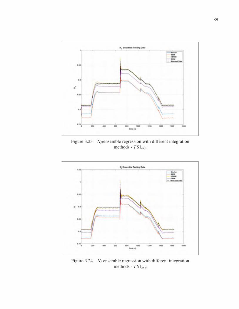
89
Figure 3.23 NHensemble regression with different integration
methods - T S1exp
Figure 3.24 NI ensemble regression with different integration
methods - T S1exp
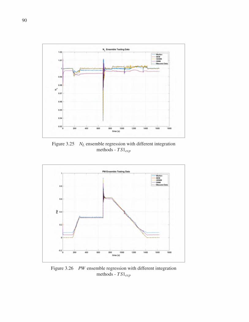
90
Figure 3.25 NL ensemble regression with different integration
methods - T S1exp
Figure 3.26 PW ensemble regression with different integration
methods - T S1exp
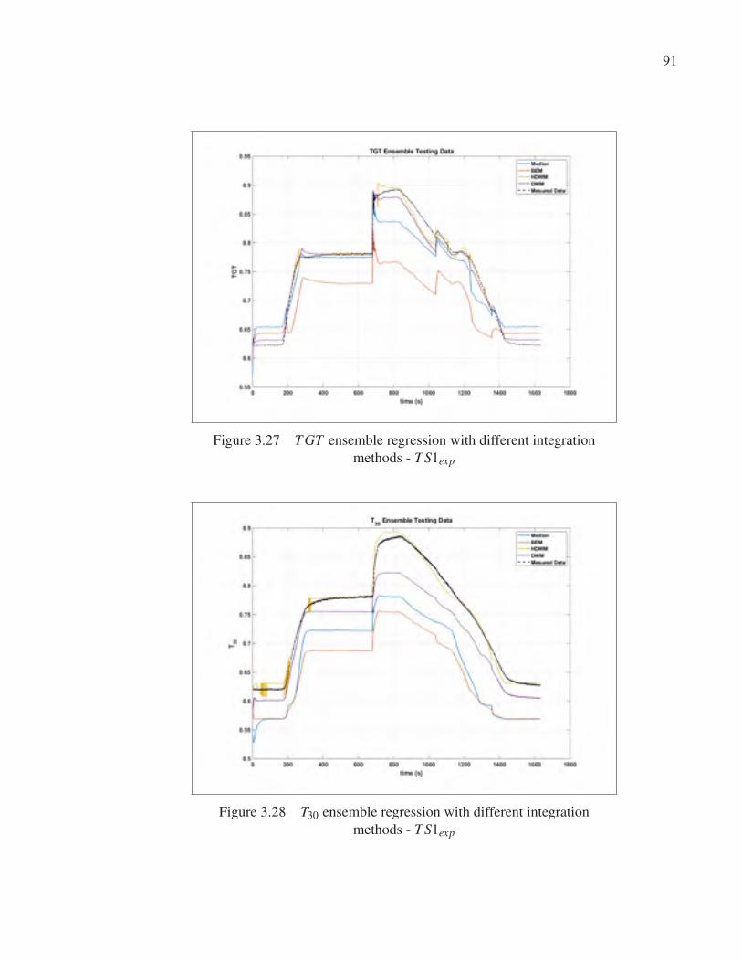
91
Figure 3.27 T GT ensemble regression with different integration
methods - T S1exp
Figure 3.28 T30 ensemble regression with different integration
methods - T S1exp
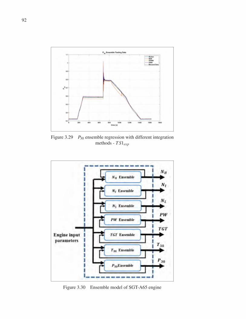
92
Figure 3.29 P30 ensemble regression with different integration
methods - T S1exp
Figure 3.30 Ensemble model of SGT-A65 engine
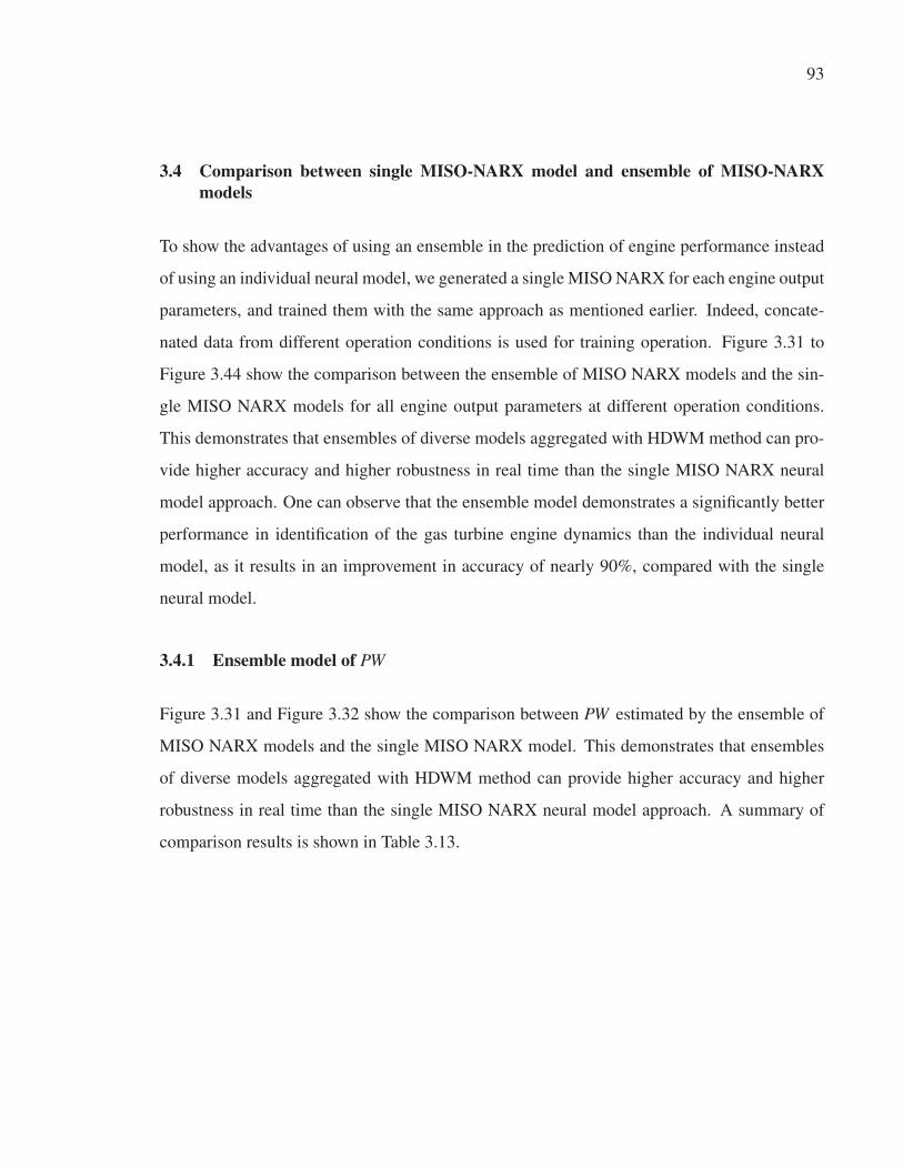
93
3.4 Comparison between single MISO-NARX model and ensemble of MISO-NARXmodels
To show the advantages of using an ensemble in the prediction of engine performance instead
of using an individual neural model, we generated a single MISO NARX for each engine output
parameters, and trained them with the same approach as mentioned earlier. Indeed, concate-
nated data from different operation conditions is used for training operation. Figure 3.31 to
Figure 3.44 show the comparison between the ensemble of MISO NARX models and the sin-
gle MISO NARX models for all engine output parameters at different operation conditions.
This demonstrates that ensembles of diverse models aggregated with HDWM method can pro-
vide higher accuracy and higher robustness in real time than the single MISO NARX neural
model approach. One can observe that the ensemble model demonstrates a significantly better
performance in identification of the gas turbine engine dynamics than the individual neural
model, as it results in an improvement in accuracy of nearly 90%, compared with the single
neural model.
3.4.1 Ensemble model of PW
Figure 3.31 and Figure 3.32 show the comparison between PW estimated by the ensemble of
MISO NARX models and the single MISO NARX model. This demonstrates that ensembles
of diverse models aggregated with HDWM method can provide higher accuracy and higher
robustness in real time than the single MISO NARX neural model approach. A summary of
comparison results is shown in Table 3.13.
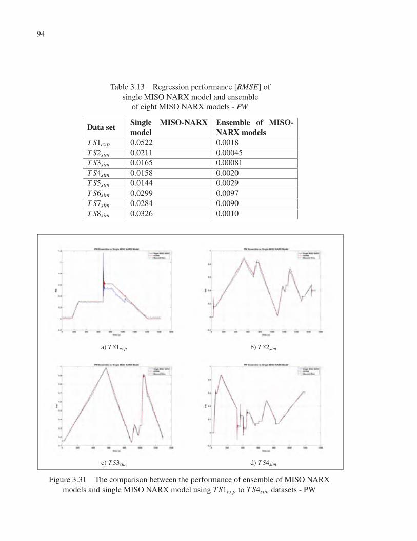
94
Table 3.13 Regression performance [RMSE] of
single MISO NARX model and ensemble
of eight MISO NARX models - PW
Data set Single MISO-NARXmodel
Ensemble of MISO-NARX models
T S1exp 0.0522 0.0018
T S2sim 0.0211 0.00045
T S3sim 0.0165 0.00081
T S4sim 0.0158 0.0020
T S5sim 0.0144 0.0029
T S6sim 0.0299 0.0097
T S7sim 0.0284 0.0090
T S8sim 0.0326 0.0010
a) T S1exp b) T S2sim
c) T S3sim d) T S4sim
Figure 3.31 The comparison between the performance of ensemble of MISO NARX
models and single MISO NARX model using T S1exp to T S4sim datasets - PW
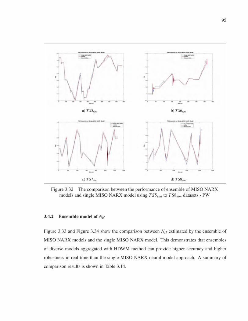
95
a) T S5sim b) T S6sim
c) T S7sim d) T S8sim
Figure 3.32 The comparison between the performance of ensemble of MISO NARX
models and single MISO NARX model using T S5sim to T S8sim datasets - PW
3.4.2 Ensemble model of NH
Figure 3.33 and Figure 3.34 show the comparison between NH estimated by the ensemble of
MISO NARX models and the single MISO NARX model. This demonstrates that ensembles
of diverse models aggregated with HDWM method can provide higher accuracy and higher
robustness in real time than the single MISO NARX neural model approach. A summary of
comparison results is shown in Table 3.14.
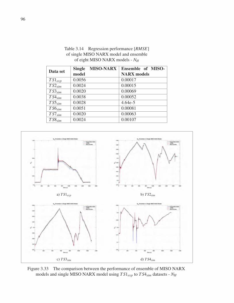
96
Table 3.14 Regression performance [RMSE]
of single MISO NARX model and ensemble
of eight MISO NARX models - NH
Data set Single MISO-NARXmodel
Ensemble of MISO-NARX models
T S1exp 0.0056 0.00017
T S2sim 0.0024 0.00015
T S3sim 0.0020 0.00069
T S4sim 0.0038 0.00052
T S5sim 0.0028 4.64e-5
T S6sim 0.0051 0.00081
T S7sim 0.0020 0.00063
T S8sim 0.0024 0.00107
a) T S1exp b) T S2sim
c) T S3sim d) T S4sim
Figure 3.33 The comparison between the performance of ensemble of MISO NARX
models and single MISO NARX model using T S1exp to T S4sim datasets - NH
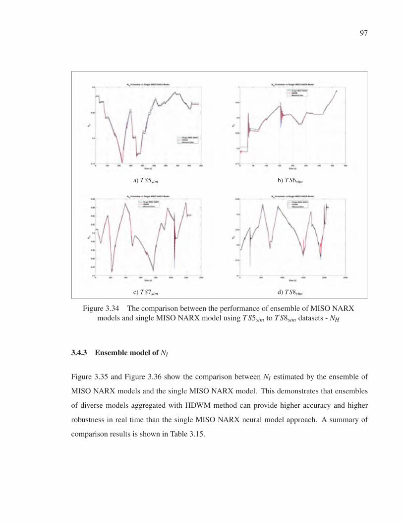
97
a) T S5sim b) T S6sim
c) T S7sim d) T S8sim
Figure 3.34 The comparison between the performance of ensemble of MISO NARX
models and single MISO NARX model using T S5sim to T S8sim datasets - NH
3.4.3 Ensemble model of NI
Figure 3.35 and Figure 3.36 show the comparison between NI estimated by the ensemble of
MISO NARX models and the single MISO NARX model. This demonstrates that ensembles
of diverse models aggregated with HDWM method can provide higher accuracy and higher
robustness in real time than the single MISO NARX neural model approach. A summary of
comparison results is shown in Table 3.15.
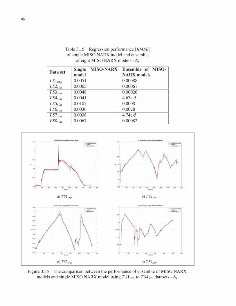
98
Table 3.15 Regression performance [RMSE]
of single MISO NARX model and ensemble
of eight MISO NARX models - NI
Data set Single MISO-NARXmodel
Ensemble of MISO-NARX models
T S1exp 0.0051 0.00088
T S2sim 0.0065 0.00061
T S3sim 0.0048 0.00026
T S4sim 0.0041 4.67e-5
T S5sim 0.0107 0.0008
T S6sim 0.0036 0.0028
T S7sim 0.0038 4.74e-5
T S8sim 0.0067 0.00082
a) T S1exp b) T S2sim
c) T S3sim d) T S4sim
Figure 3.35 The comparison between the performance of ensemble of MISO NARX
models and single MISO NARX model using T S1exp to T S4sim datasets - NI
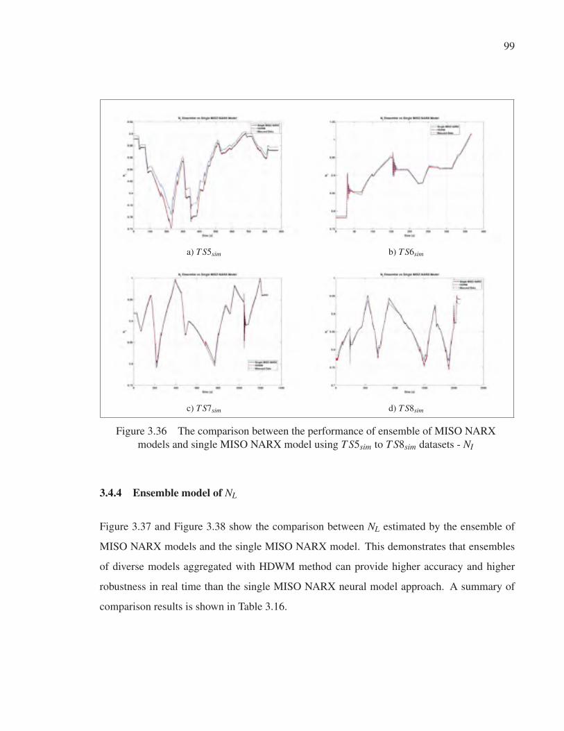
99
a) T S5sim b) T S6sim
c) T S7sim d) T S8sim
Figure 3.36 The comparison between the performance of ensemble of MISO NARX
models and single MISO NARX model using T S5sim to T S8sim datasets - NI
3.4.4 Ensemble model of NL
Figure 3.37 and Figure 3.38 show the comparison between NL estimated by the ensemble of
MISO NARX models and the single MISO NARX model. This demonstrates that ensembles
of diverse models aggregated with HDWM method can provide higher accuracy and higher
robustness in real time than the single MISO NARX neural model approach. A summary of
comparison results is shown in Table 3.16.
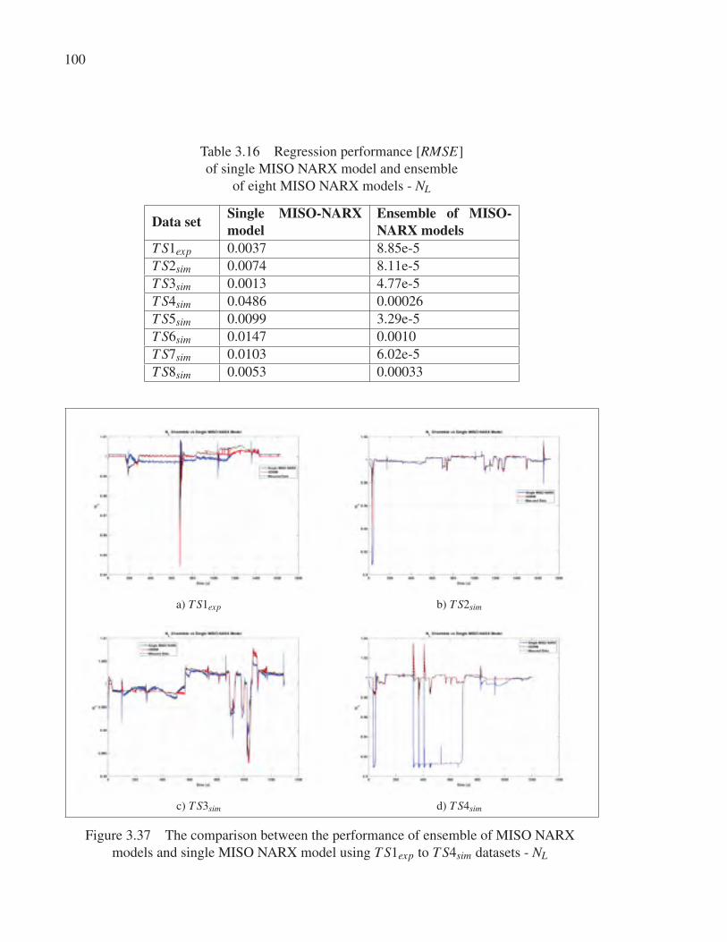
100
Table 3.16 Regression performance [RMSE]
of single MISO NARX model and ensemble
of eight MISO NARX models - NL
Data set Single MISO-NARXmodel
Ensemble of MISO-NARX models
T S1exp 0.0037 8.85e-5
T S2sim 0.0074 8.11e-5
T S3sim 0.0013 4.77e-5
T S4sim 0.0486 0.00026
T S5sim 0.0099 3.29e-5
T S6sim 0.0147 0.0010
T S7sim 0.0103 6.02e-5
T S8sim 0.0053 0.00033
a) T S1exp b) T S2sim
c) T S3sim d) T S4sim
Figure 3.37 The comparison between the performance of ensemble of MISO NARX
models and single MISO NARX model using T S1exp to T S4sim datasets - NL
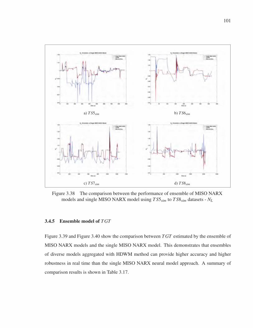
101
a) T S5sim b) T S6sim
c) T S7sim d) T S8sim
Figure 3.38 The comparison between the performance of ensemble of MISO NARX
models and single MISO NARX model using T S5sim to T S8sim datasets - NL
3.4.5 Ensemble model of T GT
Figure 3.39 and Figure 3.40 show the comparison between T GT estimated by the ensemble of
MISO NARX models and the single MISO NARX model. This demonstrates that ensembles
of diverse models aggregated with HDWM method can provide higher accuracy and higher
robustness in real time than the single MISO NARX neural model approach. A summary of
comparison results is shown in Table 3.17.
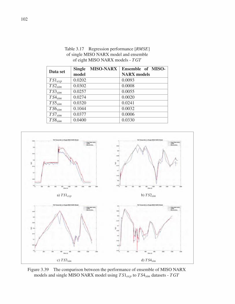
102
Table 3.17 Regression performance [RMSE]
of single MISO NARX model and ensemble
of eight MISO NARX models - T GT
Data set Single MISO-NARXmodel
Ensemble of MISO-NARX models
T S1exp 0.0202 0.0093
T S2sim 0.0302 0.0008
T S3sim 0.0257 0.0055
T S4sim 0.0274 0.0020
T S5sim 0.0320 0.0241
T S6sim 0.1044 0.0032
T S7sim 0.0377 0.0006
T S8sim 0.0400 0.0330
a) T S1exp b) T S2sim
c) T S3sim d) T S4sim
Figure 3.39 The comparison between the performance of ensemble of MISO NARX
models and single MISO NARX model using T S1exp to T S4sim datasets - T GT
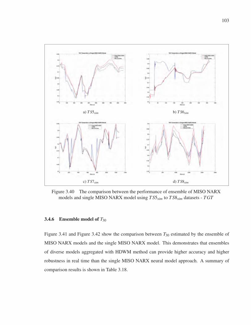
103
a) T S5sim b) T S6sim
c) T S7sim d) T S8sim
Figure 3.40 The comparison between the performance of ensemble of MISO NARX
models and single MISO NARX model using T S5sim to T S8sim datasets - T GT
3.4.6 Ensemble model of T30
Figure 3.41 and Figure 3.42 show the comparison between T30 estimated by the ensemble of
MISO NARX models and the single MISO NARX model. This demonstrates that ensembles
of diverse models aggregated with HDWM method can provide higher accuracy and higher
robustness in real time than the single MISO NARX neural model approach. A summary of
comparison results is shown in Table 3.18.
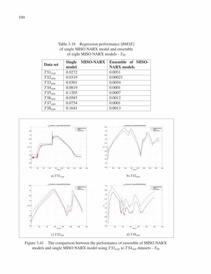
104
Table 3.18 Regression performance [RMSE]
of single MISO NARX model and ensemble
of eight MISO NARX models - T30
Data set Single MISO-NARXmodel
Ensemble of MISO-NARX models
T S1exp 0.0272 0.0031
T S2sim 0.0319 0.00021
T S3sim 0.0301 0.0054
T S4sim 0.0819 0.0001
T S5sim 0.1205 0.0007
T S6sim 0.0585 0.0012
T S7sim 0.0754 0.0001
T S8sim 0.1641 0.0013
a) T S1exp b) T S2sim
c) T S3sim d) T S4sim
Figure 3.41 The comparison between the performance of ensemble of MISO NARX
models and single MISO NARX model using T S1exp to T S4sim datasets - T30
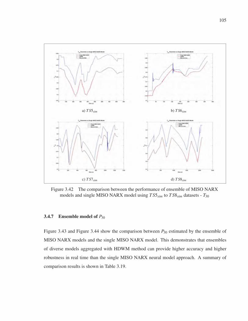
105
a) T S5sim b) T S6sim
c) T S7sim d) T S8sim
Figure 3.42 The comparison between the performance of ensemble of MISO NARX
models and single MISO NARX model using T S5sim to T S8sim datasets - T30
3.4.7 Ensemble model of P30
Figure 3.43 and Figure 3.44 show the comparison between P30 estimated by the ensemble of
MISO NARX models and the single MISO NARX model. This demonstrates that ensembles
of diverse models aggregated with HDWM method can provide higher accuracy and higher
robustness in real time than the single MISO NARX neural model approach. A summary of
comparison results is shown in Table 3.19.
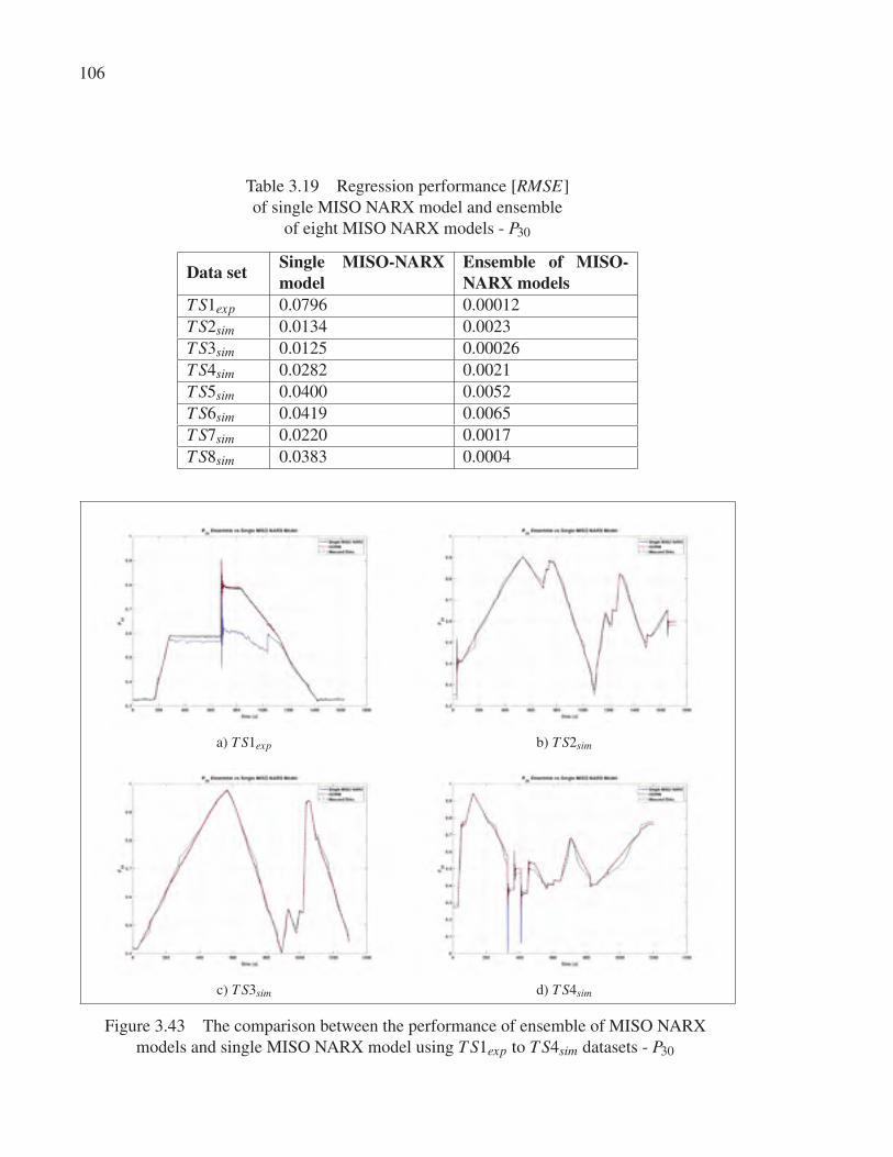
106
Table 3.19 Regression performance [RMSE]
of single MISO NARX model and ensemble
of eight MISO NARX models - P30
Data set Single MISO-NARXmodel
Ensemble of MISO-NARX models
T S1exp 0.0796 0.00012
T S2sim 0.0134 0.0023
T S3sim 0.0125 0.00026
T S4sim 0.0282 0.0021
T S5sim 0.0400 0.0052
T S6sim 0.0419 0.0065
T S7sim 0.0220 0.0017
T S8sim 0.0383 0.0004
a) T S1exp b) T S2sim
c) T S3sim d) T S4sim
Figure 3.43 The comparison between the performance of ensemble of MISO NARX
models and single MISO NARX model using T S1exp to T S4sim datasets - P30
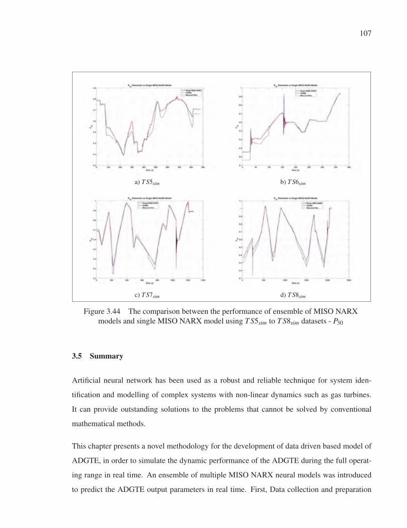
107
a) T S5sim b) T S6sim
c) T S7sim d) T S8sim
Figure 3.44 The comparison between the performance of ensemble of MISO NARX
models and single MISO NARX model using T S5sim to T S8sim datasets - P30
3.5 Summary
Artificial neural network has been used as a robust and reliable technique for system iden-
tification and modelling of complex systems with non-linear dynamics such as gas turbines.
It can provide outstanding solutions to the problems that cannot be solved by conventional
mathematical methods.
This chapter presents a novel methodology for the development of data driven based model of
ADGTE, in order to simulate the dynamic performance of the ADGTE during the full operat-
ing range in real time. An ensemble of multiple MISO NARX neural models was introduced
to predict the ADGTE output parameters in real time. First, Data collection and preparation
108
was performed, which includes collection of closed loop data from operational testing of the
SGT-A65 ADGTE and the high fidelity simulation program of Siemens at different operation
conditions. After that, data cleaning and re-sampling was performed to generate eight datasets
for system identification. Secondly, estimation of the system order and delay were done by
identification of linear ARX models based on the experimental datasets. This represents a key
step before identification of the non-linear neural model. Third, the NARX neural network
was chosen to be a base model of the ensemble of ADGTE due to its capability in the simu-
lation and prediction of the response of non-linear systems. Moreover, multiple MISO NARX
models for each output parameter from the ADGTE were generated. Each NARX model has a
configuration that is different from the other ones and is based on the function of this model.
A comprehensive computer program was used to select the best structure of MISO NARX
model for each output parameter. After that, retraining operation of the selected MISO-NARX
models was performed with training datasets from different operation conditions. As a result,
seven homogeneous ensembles each one consisting of eight MISO NARX models were devel-
oped to predict the seven output parameters from the ADGTE at different operation conditions.
The last and most important step in the ensemble generation is the combination of the outputs
from the eight diverse models in each ensemble. A novel hybrid dynamic weighting method
(HDWM) was proposed to perform this task, and verification of this method was performed
by comparing its outputs with the output from three common integration methods. The results
presented a superior performance of the new integration method. Finally, testing of the gener-
ated ensembles which use the HDWM method was performed at different operation conditions
to measure the prediction accuracy and generalization property of the ensembles.
As shown in the results, the ensemble of MISO-NARX models can represent the ADGTE dur-
ing the full operating range with a good accuracy even with different input scenarios from dif-
ferent operation conditions which prove the high generalization characteristic of the ensemble.
Also, another important gain was the very low execution time (40.5 μs as compared to more
than 10 ms using the same real time machine), which can support many real time applications
like model based controller design, sensor fault verification and engine health monitoring. In

109
this study, this model will be used to design a model based controller to improve the perfor-
mance of the ADGTE.
On the other hand, estimation of the NN model order by generating different ARX models
and estimation of the input/output delay, before generation of NN model, are very important
steps. These steps save more iterations required to find the best structure of the NN and con-
sequently save more time required for NN model generation. In addition, data cleaning and
resampling step significantly reduce training time. The lower sampling rate reduces the num-
ber of data points, which reduces the computation time during training operation and reduces
data co-linearity. In (Asgari, 2014), in order to find the best model for the gas turbine engine,
the generated code was run in MATLAB and 18720 different ANN structures were trained.
However, this number was reduced to 240 different ANN structures by using the proposed
approach.

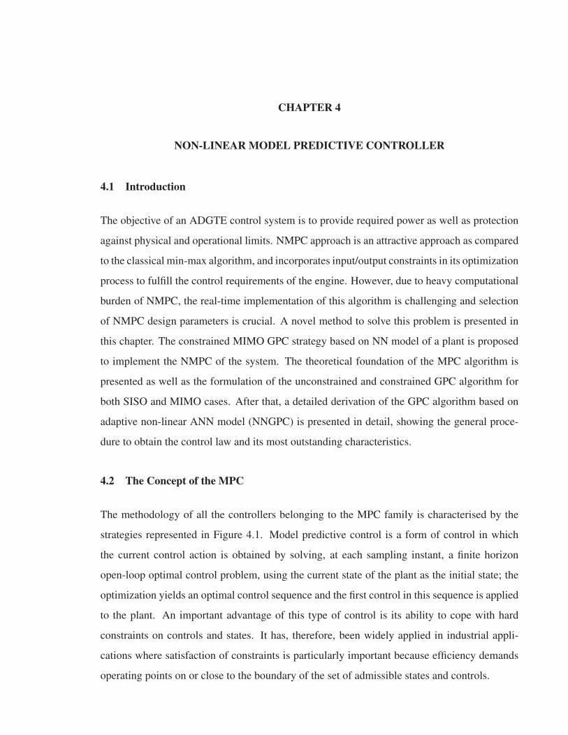
CHAPTER 4
NON-LINEAR MODEL PREDICTIVE CONTROLLER
4.1 Introduction
The objective of an ADGTE control system is to provide required power as well as protection
against physical and operational limits. NMPC approach is an attractive approach as compared
to the classical min-max algorithm, and incorporates input/output constraints in its optimization
process to fulfill the control requirements of the engine. However, due to heavy computational
burden of NMPC, the real-time implementation of this algorithm is challenging and selection
of NMPC design parameters is crucial. A novel method to solve this problem is presented in
this chapter. The constrained MIMO GPC strategy based on NN model of a plant is proposed
to implement the NMPC of the system. The theoretical foundation of the MPC algorithm is
presented as well as the formulation of the unconstrained and constrained GPC algorithm for
both SISO and MIMO cases. After that, a detailed derivation of the GPC algorithm based on
adaptive non-linear ANN model (NNGPC) is presented in detail, showing the general proce-
dure to obtain the control law and its most outstanding characteristics.
4.2 The Concept of the MPC
The methodology of all the controllers belonging to the MPC family is characterised by the
strategies represented in Figure 4.1. Model predictive control is a form of control in which
the current control action is obtained by solving, at each sampling instant, a finite horizon
open-loop optimal control problem, using the current state of the plant as the initial state; the
optimization yields an optimal control sequence and the first control in this sequence is applied
to the plant. An important advantage of this type of control is its ability to cope with hard
constraints on controls and states. It has, therefore, been widely applied in industrial appli-
cations where satisfaction of constraints is particularly important because efficiency demands
operating points on or close to the boundary of the set of admissible states and controls.
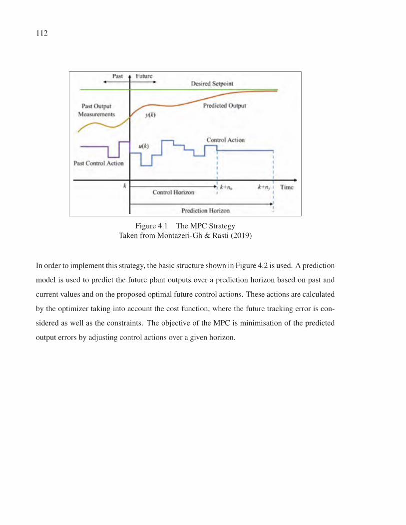
112
Figure 4.1 The MPC Strategy
Taken from Montazeri-Gh & Rasti (2019)
In order to implement this strategy, the basic structure shown in Figure 4.2 is used. A prediction
model is used to predict the future plant outputs over a prediction horizon based on past and
current values and on the proposed optimal future control actions. These actions are calculated
by the optimizer taking into account the cost function, where the future tracking error is con-
sidered as well as the constraints. The objective of the MPC is minimisation of the predicted
output errors by adjusting control actions over a given horizon.
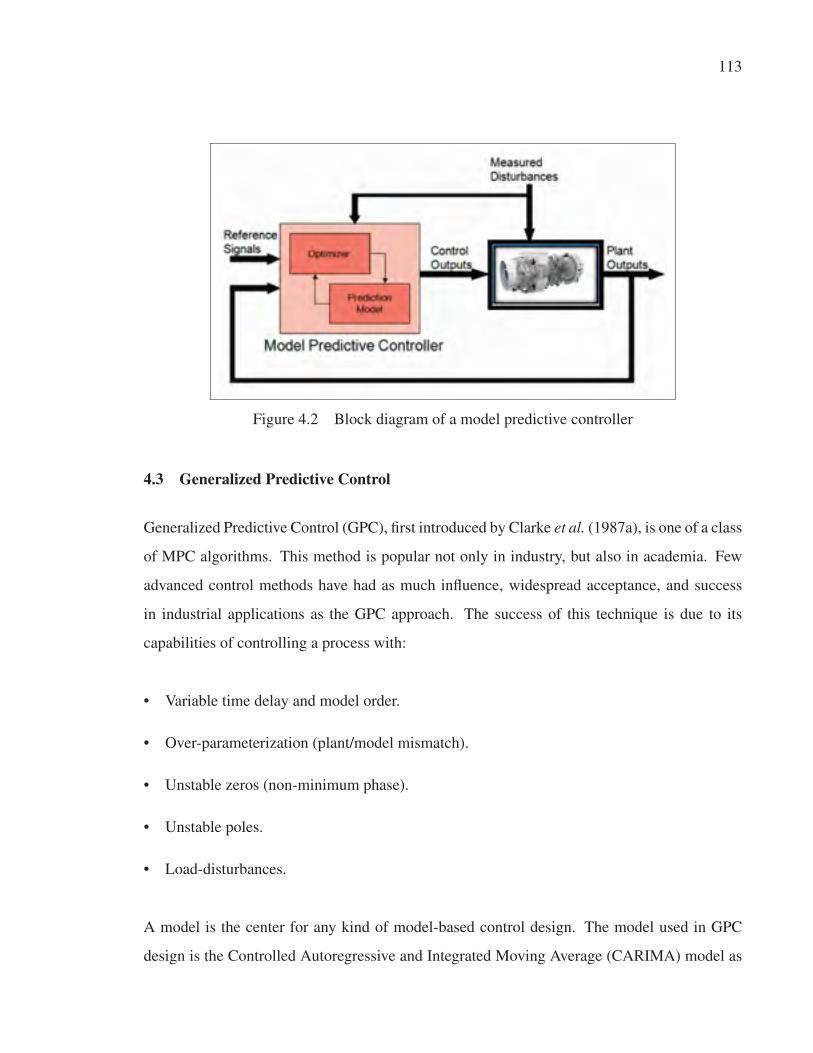
113
Figure 4.2 Block diagram of a model predictive controller
4.3 Generalized Predictive Control
Generalized Predictive Control (GPC), first introduced by Clarke et al. (1987a), is one of a class
of MPC algorithms. This method is popular not only in industry, but also in academia. Few
advanced control methods have had as much influence, widespread acceptance, and success
in industrial applications as the GPC approach. The success of this technique is due to its
capabilities of controlling a process with:
• Variable time delay and model order.
• Over-parameterization (plant/model mismatch).
• Unstable zeros (non-minimum phase).
• Unstable poles.
• Load-disturbances.
A model is the center for any kind of model-based control design. The model used in GPC
design is the Controlled Autoregressive and Integrated Moving Average (CARIMA) model as
114
shown in equation (4.1),
A(z−1)y(t) = B(z−1)u(t −1)+C(z−1)e(t)Δ
(4.1)
where y(t) is the process output, u(t) is the input , and e(t) is the white noise. The difference
operator Δ = 1− z−1 in the denominator of the noise term is widely assumed, as it forces an
integrator into the controller in order to eliminate offset between the measured output and its
set point. A(z−1), B(z−1) and C(z−1) are the polynomials in the backward-shift operator z−1
with the orders of ny, nu and nk respectively:
A(z−1) = 1+a1z−1 +a2z−2 + · · ·+anaz−ny
B(z−1) = b0 +b1z−1 +b2z−2 + · · ·+bnbz−nu
C(z−1) = 1+b1z−1 + c2z−2 + · · ·+ cncz−nk
(4.2)
The GPC strategy is based on applying a control sequence that minimizes a quadratic cost
function measuring the control effort and the distance between the predicted system output and
desired outputs over the prediction horizon, i.e.
J (N1,N2,Nu) =N2
∑j=N1
[y(t + j|t)−w(t + j)]2 +ΛNu
∑j=1
[Δu(t + j−1)]2 (4.3)
subjected to Δu(t + j) = 0 when j > Nu
where y is the predicted output from the system model, and w is the reference output. u(t + j−1) is the sequence of future control action that is to be determined. N1, N2 are the minimum,
maximum horizon, and Nu is the control horizon. Λ is a weighting factor penalizing changes in
the control inputs. The tuning parameters of the GPC are N1, N2, Nu, and Λ, which determine
the stability and performance of the GPC controller. Notice that, N1 ≥ 1, N2 ≥ N1, and N2 ≥Nu ≥ 1 . In addition, some guidelines for selecting those parameters exist in (Clarke et al.,
1987b; Clarke & Mohtadi, 1987).
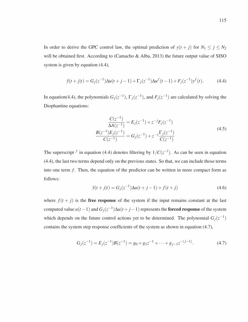
115
In order to derive the GPC control law, the optimal prediction of y(t + j) for N1 ≤ j ≤ N2
will be obtained first. According to (Camacho & Alba, 2013) the future output value of SISO
system is given by equation (4.4),
y(t + j|t) = G j(z−1)Δu(t + j−1)+Γ j(z−1)Δu f (t −1)+Fj(z−1)y f (t). (4.4)
In equation(4.4), the polynomials G j(z−1), Γ j(z−1), and Fj(z−1) are calculated by solving the
Diophantine equations:
C(z−1)
ΔA(z−1)= E j(z−1)+ z− jFj(z−1)
B(z−1)E j(z−1)
C(z−1)= G j(z−1)+ z− j Γ j(z−1)
C(z−1)
(4.5)
The superscript f in equation (4.4) denotes filtering by 1/C(z−l). As can be seen in equation
(4.4), the last two terms depend only on the previous states. So that, we can include those terms
into one term f . Then, the equation of the predictor can be written in more compact form as
follows:
y(t + j|t) = G j(z−1)Δu(t + j−1)+ f (t + j) (4.6)
where f (t + j) is the free response of the system if the input remains constant at the last
computed value u(t−1) and G j(z−1)Δu(t+ j−1) represents the forced response of the system
which depends on the future control actions yet to be determined. The polynomial G j(z−1)
contains the system step response coefficients of the system as shown in equation (4.7),
G j(z−1) = E j(z−1)B(z−1) = g0 +g1z−1 + · · ·+g j−1z−( j−1). (4.7)

116
To simplify the following derivation of the GPC control law, let N1 = 1. Now consider the
following set of j step ahead optimal predictions:
y(t +1|t) = G1(z−1)Δu(t)+ f (t +1)
y(t +2|t) = G2(z−1)Δu(t +1)+ f (t +2)
...
y(t +N2|t) = GN2(z−1)Δu(t +N2 −1)+ f (t +N2)
(4.8)
Hence, the predictor in vector notation can be written as:
y = GΔu+ f (4.9)
where
y =
⎡⎢⎢⎢⎢⎢⎢⎣
y(t +1|t)y(t +2|t)
...
y(t +N2|t)
⎤⎥⎥⎥⎥⎥⎥⎦[N2X1]
, Δ u =
⎡⎢⎢⎢⎢⎢⎢⎣
Δu(t)
Δu(t +1)...
Δu(t +Nu −1)
⎤⎥⎥⎥⎥⎥⎥⎦[NuX1]
,
f =
⎡⎢⎢⎢⎢⎢⎢⎣
f (t +1)
f (t +2)...
f (t +N2)
⎤⎥⎥⎥⎥⎥⎥⎦[N2X1]
& G =
⎡⎢⎢⎢⎢⎢⎢⎢⎢⎢⎢⎢⎢⎣
g0 0 · · · 0
g1 g0 · · · 0...
......
...
gNu−1 · · · g1 g0
......
......
gN2−1 gN2−2 · · · gN2−Nu
⎤⎥⎥⎥⎥⎥⎥⎥⎥⎥⎥⎥⎥⎦[N2XNu]
For SISO systems, the matrix G is a lower triangular matrix of dimension [N2XNu]. Besides,
the first column of G can be calculated as the step response of the system when a unit step is
applied to the manipulated variable.
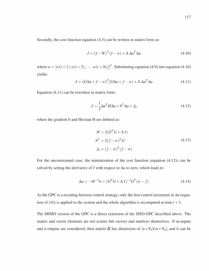
117
Secondly, the cost function equation (4.3) can be written in matrix form as:
J = (y−W )T (y−w)+Λ ΔuT Δu (4.10)
where w = [w(t+1),w(t+2), · · · ,w(t+N2)]T . Substituting equation (4.9) into equation (4.10)
yields:
J = (GΔu+ f −w)T (GΔu+ f −w)+Λ ΔuT Δu (4.11)
Equation (4.11) can be rewritten in matrix form:
J =1
2ΔuT HΔu+bT Δu+ f0 (4.12)
where the gradient b and Hessian H are defined as:
H = 2(GT G+Λ I)
bT = 2( f −w)T G
f0 = ( f −w)T ( f −w)
(4.13)
For the unconstrained case, the minimization of the cost function (equation (4.12)) can be
solved by setting the derivative of J with respect to Δu to zero, which leads to:
Δu =−H−1b = (GT G+Λ I)−1GT (w− f ) (4.14)
As the GPC is a receding-horizon control strategy, only the first control increment in Δu (equa-
tion (4.14)) is applied to the system and the whole algorithm is recomputed at time t +1.
The MIMO version of the GPC is a direct extension of the SISO GPC described above. The
matrix and vector elements are not scalars but vectors and matrices themselves. If m-inputs
and n-outputs are considered, then matrix GGG has dimension of [n ∗N2Xm ∗Nu], and it can be
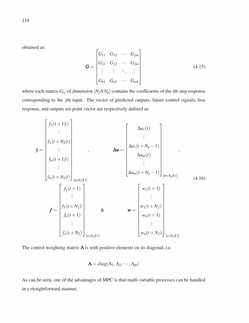
118
obtained as:
GGG =
⎡⎢⎢⎢⎢⎢⎢⎣
G11 G12 · · · G1m
G21 G22 · · · G2m...
.... . .
...
Gn1 Gn2 · · · Gnm
⎤⎥⎥⎥⎥⎥⎥⎦
(4.15)
where each matrix Gi j of dimension [N2XNu] contains the coefficients of the ith step response
corresponding to the jth input. The vector of predicted outputs, future control signals, free
response, and outputs set-point vector are respectively defined as:
yyy =
⎡⎢⎢⎢⎢⎢⎢⎢⎢⎢⎢⎢⎢⎢⎢⎢⎣
y1(t +1|t)...
y1(t +N2|t)...
yn(t +1|t)...
yn(t +N2|t)
⎤⎥⎥⎥⎥⎥⎥⎥⎥⎥⎥⎥⎥⎥⎥⎥⎦[n∗N2X1]
, ΔΔΔuuu =
⎡⎢⎢⎢⎢⎢⎢⎢⎢⎢⎢⎢⎢⎣
Δu1(t)...
Δu1(t +Nu −1)
Δum(t)...
Δum(t +Nu −1)
⎤⎥⎥⎥⎥⎥⎥⎥⎥⎥⎥⎥⎥⎦[m∗NuX1]
,
fff =
⎡⎢⎢⎢⎢⎢⎢⎢⎢⎢⎢⎢⎢⎣
f1(t +1)...
f1(t +N2)...
fn(t +1)...
fn(t +N2)
⎤⎥⎥⎥⎥⎥⎥⎥⎥⎥⎥⎥⎥⎦[n∗N2X1]
& www =
⎡⎢⎢⎢⎢⎢⎢⎢⎢⎢⎢⎢⎢⎣
w1(t +1)...
w1(t +N2)...
wn(t +1)...
wn(t +N2)
⎤⎥⎥⎥⎥⎥⎥⎥⎥⎥⎥⎥⎥⎦[n∗N2X1]
(4.16)
The control weighting matrix ΛΛΛ is with positive elements on its diagonal, i.e.
ΛΛΛ = diag(Λ1,Λ2, · · · ,Λm)
As can be seen, one of the advantages of MPC is that multi-variable processes can be handled
in a straightforward manner.
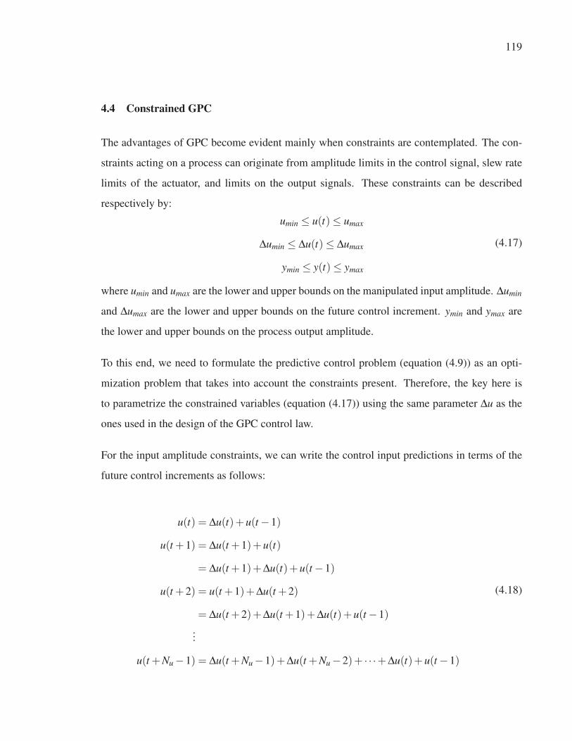
119
4.4 Constrained GPC
The advantages of GPC become evident mainly when constraints are contemplated. The con-
straints acting on a process can originate from amplitude limits in the control signal, slew rate
limits of the actuator, and limits on the output signals. These constraints can be described
respectively by:
umin ≤ u(t)≤ umax
Δumin ≤ Δu(t)≤ Δumax
ymin ≤ y(t)≤ ymax
(4.17)
where umin and umax are the lower and upper bounds on the manipulated input amplitude. Δumin
and Δumax are the lower and upper bounds on the future control increment. ymin and ymax are
the lower and upper bounds on the process output amplitude.
To this end, we need to formulate the predictive control problem (equation (4.9)) as an opti-
mization problem that takes into account the constraints present. Therefore, the key here is
to parametrize the constrained variables (equation (4.17)) using the same parameter Δu as the
ones used in the design of the GPC control law.
For the input amplitude constraints, we can write the control input predictions in terms of the
future control increments as follows:
u(t) = Δu(t)+u(t −1)
u(t +1) = Δu(t +1)+u(t)
= Δu(t +1)+Δu(t)+u(t −1)
u(t +2) = u(t +1)+Δu(t +2)
= Δu(t +2)+Δu(t +1)+Δu(t)+u(t −1)
...
u(t +Nu −1) = Δu(t +Nu −1)+Δu(t +Nu −2)+ · · ·+Δu(t)+u(t −1)
(4.18)

120
Now, the input amplitude constraints over the control horizon Nu can be rewritten as follows:
The input amplitude constraint at time t is:
umin ≤ u(t)≤ umax (4.19)
Replacing u(t) with Δu(t)+u(t −1) from equation (4.18)) and re-arranging the terms yields:
umin −u(t −1)≤ Δu(t)≤ umax −u(t −1) (4.20)
Advancing t by one step gives:
umin ≤ u(t +1)≤ umax
umin −u(t −1)≤ Δu(t +1)+Δu(t)≤ umax −u(t −1)(4.21)
Advancing t+1 by one step once more and performing the same substitution gives:
umin ≤ u(t +2)≤ umax
umin −u(t −1)≤ Δu(t +2)+Δu(t +1)+Δu(t)≤ umax −u(t −1)(4.22)
A clear pattern arises, allowing us to write the entire set of input constraints over the control
horizon Nu in matrix form as follows:
(umin −u(t −1))
⎡⎢⎢⎢⎢⎢⎢⎣
1
1...
1
⎤⎥⎥⎥⎥⎥⎥⎦≤
⎡⎢⎢⎢⎢⎢⎢⎣
1 0 0 · · ·1 1 0 · · ·...
......
...
1 1 1 · · ·
⎤⎥⎥⎥⎥⎥⎥⎦
⎡⎢⎢⎢⎢⎢⎢⎣
Δu(t)
Δu(t +1)...
Δu(t +Nu −1)
⎤⎥⎥⎥⎥⎥⎥⎦≤
⎡⎢⎢⎢⎢⎢⎢⎣
1
1...
1
⎤⎥⎥⎥⎥⎥⎥⎦(umax −u(t −1))
(4.23)
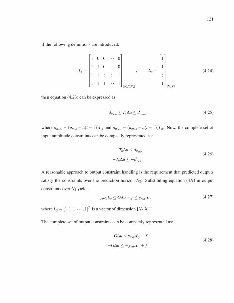
121
If the following definitions are introduced:
Tu =
⎡⎢⎢⎢⎢⎢⎢⎣
1 0 0 · · · 0
1 1 0 · · · 0...
......
......
1 1 1 · · · 1
⎤⎥⎥⎥⎥⎥⎥⎦[NuXNu]
, Lu =
⎡⎢⎢⎢⎢⎢⎢⎣
1
1...
1
⎤⎥⎥⎥⎥⎥⎥⎦[NuX1]
(4.24)
then equation (4.23) can be expressed as:
dumin ≤ TuΔu ≤ dumax (4.25)
where dumin = (umin − u(t − 1))Lu and dumax = (umax − u(t − 1))Lu. Now, the complete set of
input amplitude constraints can be compactly represented as:
TuΔu ≤ dumax
−TuΔu ≤−dumin
(4.26)
A reasonable approach to output constraint handling is the requirement that predicted outputs
satisfy the constraints over the prediction horizon N2. Substituting equation (4.9) in output
constraints over N2 yields:
yminLy ≤ GΔu+ f ≤ ymaxLy (4.27)
where Ly = [1,1,1, · · · ,1]T is a vector of dimension [N2 X 1].
The complete set of output constraints can be compactly represented as:
GΔu ≤ ymaxLy − f
−GΔu ≤−yminLy + f(4.28)
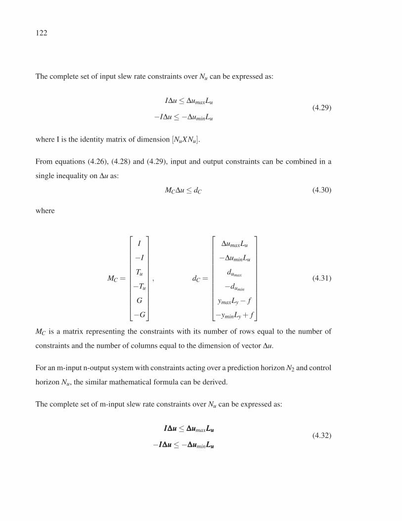
122
The complete set of input slew rate constraints over Nu can be expressed as:
IΔu ≤ ΔumaxLu
−IΔu ≤−ΔuminLu
(4.29)
where I is the identity matrix of dimension [NuXNu].
From equations (4.26), (4.28) and (4.29), input and output constraints can be combined in a
single inequality on Δu as:
MCΔu ≤ dC (4.30)
where
MC =
⎡⎢⎢⎢⎢⎢⎢⎢⎢⎢⎢⎢⎢⎣
I
−I
Tu
−Tu
G
−G
⎤⎥⎥⎥⎥⎥⎥⎥⎥⎥⎥⎥⎥⎦, dC =
⎡⎢⎢⎢⎢⎢⎢⎢⎢⎢⎢⎢⎢⎣
ΔumaxLu
−ΔuminLu
dumax
−dumin
ymaxLy − f
−yminLy + f
⎤⎥⎥⎥⎥⎥⎥⎥⎥⎥⎥⎥⎥⎦
(4.31)
MC is a matrix representing the constraints with its number of rows equal to the number of
constraints and the number of columns equal to the dimension of vector Δu.
For an m-input n-output system with constraints acting over a prediction horizon N2 and control
horizon Nu, the similar mathematical formula can be derived.
The complete set of m-input slew rate constraints over Nu can be expressed as:
IIIΔΔΔuuu ≤ ΔΔΔuuumaxLLLuuu
−IIIΔΔΔuuu ≤−ΔΔΔuuuminLLLuuu
(4.32)
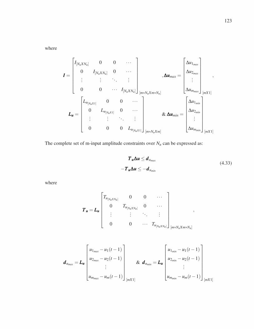
123
where
III =
⎡⎢⎢⎢⎢⎢⎢⎣
I[NuXNu] 0 0 · · ·0 I[NuXNu] 0 · · ·...
.... . .
...
0 0 · · · I[NuXNu]
⎤⎥⎥⎥⎥⎥⎥⎦[m∗NuXm∗Nu]
,ΔΔΔuuumax =
⎡⎢⎢⎢⎢⎢⎢⎣
Δu1max
Δu2max
...
Δummax
⎤⎥⎥⎥⎥⎥⎥⎦[mX1]
,
LLLuuu =
⎡⎢⎢⎢⎢⎢⎢⎣
Lu[NuX1]0 0 · · ·
0 Lu[NuX1]0 · · ·
......
. . ....
0 0 0 Lu[NuX1]
⎤⎥⎥⎥⎥⎥⎥⎦[m∗NuXm]
& ΔΔΔuuumin =
⎡⎢⎢⎢⎢⎢⎢⎣
Δu1min
Δu2min...
Δummin
⎤⎥⎥⎥⎥⎥⎥⎦[mX1]
The complete set of m-input amplitude constraints over Nu can be expressed as:
TTT uuuΔΔΔuuu ≤ dddumax
−TTT uuuΔΔΔuuu ≤−dddumin
(4.33)
where
TTT uuu = LLLuuu
⎡⎢⎢⎢⎢⎢⎢⎣
Tu[NuXNu]0 0 · · ·
0 Tu[NuXNu]0 · · ·
......
. . ....
0 0 · · · Tu[NuXNu]
⎤⎥⎥⎥⎥⎥⎥⎦[m∗NuXm∗Nu]
,
dddumax = LLLuuu
⎡⎢⎢⎢⎢⎢⎢⎣
u1max −u1(t −1)
u2max −u2(t −1)...
ummax −um(t −1)
⎤⎥⎥⎥⎥⎥⎥⎦[mX1]
& dddumin = LLLuuu
⎡⎢⎢⎢⎢⎢⎢⎣
u1min −u1(t −1)
u2min −u2(t −1)...
ummin −um(t −1)
⎤⎥⎥⎥⎥⎥⎥⎦[mX1]
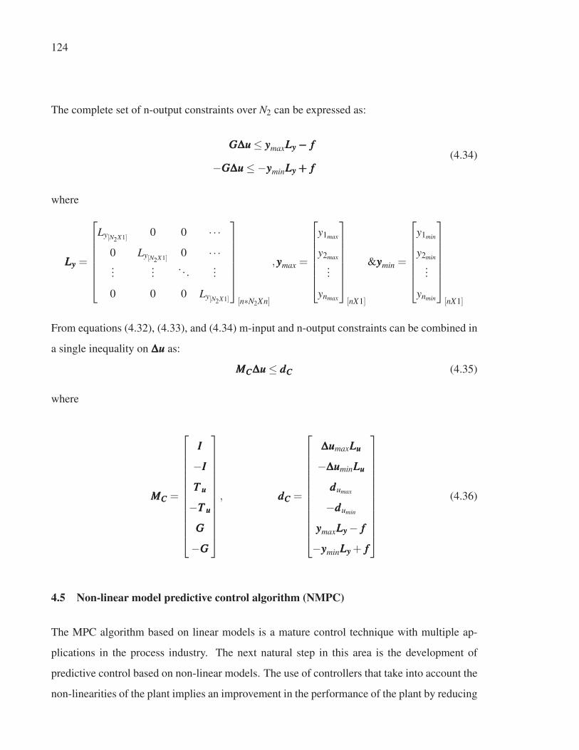
124
The complete set of n-output constraints over N2 can be expressed as:
GGGΔΔΔuuu ≤ yyymaxLLLyyy −−− fff
−GGGΔΔΔuuu ≤−yyyminLLLyyy +++ fff(4.34)
where
LLLyyy =
⎡⎢⎢⎢⎢⎢⎢⎣
Ly[N2X1]0 0 · · ·
0 Ly[N2X1]0 · · ·
......
. . ....
0 0 0 Ly[N2X1]
⎤⎥⎥⎥⎥⎥⎥⎦[n∗N2Xn]
,yyymax =
⎡⎢⎢⎢⎢⎢⎢⎣
y1max
y2max
...
ynmax
⎤⎥⎥⎥⎥⎥⎥⎦[nX1]
&yyymin =
⎡⎢⎢⎢⎢⎢⎢⎣
y1min
y2min...
ynmin
⎤⎥⎥⎥⎥⎥⎥⎦[nX1]
From equations (4.32), (4.33), and (4.34) m-input and n-output constraints can be combined in
a single inequality on ΔΔΔuuu as:
MMMCCCΔΔΔuuu ≤ dddCCC (4.35)
where
MMMCCC =
⎡⎢⎢⎢⎢⎢⎢⎢⎢⎢⎢⎢⎢⎣
III
−III
TTT uuu
−TTT uuu
GGG
−GGG
⎤⎥⎥⎥⎥⎥⎥⎥⎥⎥⎥⎥⎥⎦, dddCCC =
⎡⎢⎢⎢⎢⎢⎢⎢⎢⎢⎢⎢⎢⎣
ΔΔΔuuumaxLLLuuu
−ΔΔΔuuuminLLLuuu
dddumax
−dddumin
yyymaxLLLyyy − fff
−yyyminLLLyyy + fff
⎤⎥⎥⎥⎥⎥⎥⎥⎥⎥⎥⎥⎥⎦
(4.36)
4.5 Non-linear model predictive control algorithm (NMPC)
The MPC algorithm based on linear models is a mature control technique with multiple ap-
plications in the process industry. The next natural step in this area is the development of
predictive control based on non-linear models. The use of controllers that take into account the
non-linearities of the plant implies an improvement in the performance of the plant by reducing
125
the impact of the disturbances and by improving the tracking capabilities of the control system.
However, the usage of a non-linear model within the NMPC changes the control problem from
a convex quadratic problem to a nonconvex non-linear one. Furthermore, in this situation, there
is no guarantee that the global optimum can be found especially in real-time control when the
optimum solution has to be obtained in a prescribed time. Therefore, a novel method that tries
to avoid these problems has been presented in the following parts of this chapter.
4.5.1 The neural network generalized predictive controller (NNGPC)
An investigation of a novel approach to implement the NMPC based on neural network model
is reported in this study. A constrained MIMO NMPC is developed based on the GPC algorithm
because of its simplicity, ease of use, and ability to handle problems in one algorithm. Future
control actions are determined by minimizing the predicted errors without violating input and
output constraints. The NN model, which was generated in the previous chapter, is used as a
base model for the GPC controller to predict the future process outputs.
The design of the GPC demands the construction of a predictor (equation (4.9)). Hence, for the
calculation of the predicted future output y only two characteristics of the system are needed:
step (forced) and free responses. To obtain the step and the free process responses which are
needed in the generalized predictive control strategy we iteratively use an ensemble of MISO-
NARX models as a multi-step-ahead predictor.
The proposed control scheme in Figure 4.3 consists of a non-linear NN model of the system to
be controlled in the form of ensembles of MISO-NARX models and the GPC algorithm block.
The neural model is trained off-line as shown in the previous chapter. This model works as a
predictor which produces the free and forced responses, that are used as an input to the GPC
algorithm block. The GPC algorithm produces an output that is either used as an input to the
plant or the predictor. The double pole double throw switch, S, is set to the plant when the
GPC algorithm has solved for the best control input, u(k), that will minimize a specified cost
function. Between samples, the switch is set to the predictor where the GPC algorithm uses
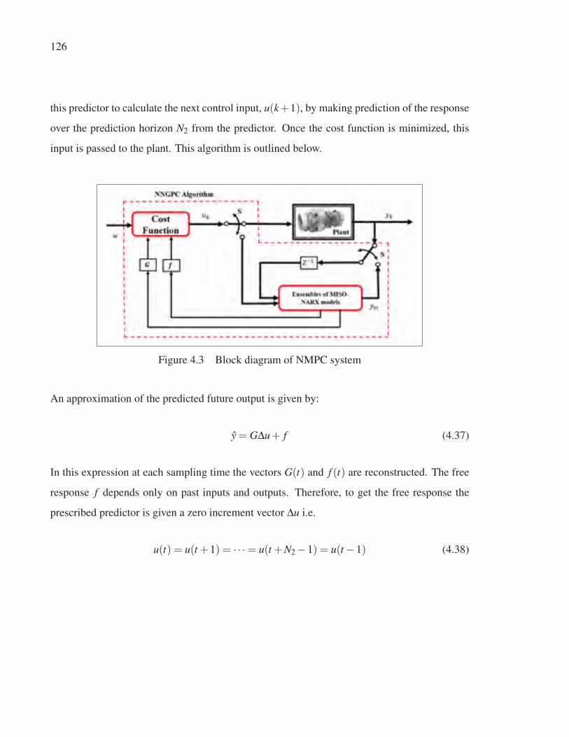
126
this predictor to calculate the next control input, u(k+1), by making prediction of the response
over the prediction horizon N2 from the predictor. Once the cost function is minimized, this
input is passed to the plant. This algorithm is outlined below.
Figure 4.3 Block diagram of NMPC system
An approximation of the predicted future output is given by:
y = GΔu+ f (4.37)
In this expression at each sampling time the vectors G(t) and f (t) are reconstructed. The free
response f depends only on past inputs and outputs. Therefore, to get the free response the
prescribed predictor is given a zero increment vector Δu i.e.
u(t) = u(t +1) = · · ·= u(t +N2 −1) = u(t −1) (4.38)
127
Hence, the predictor (ensembles of MISO-NARX models) output will be the system free re-
sponse.
y f ree(t + i|t) = F(y(t + i−1), · · · ,y(t + i−ny), · · · ,u(t + i−1), · · · ,u(t + i−nu))
with : u(k) =
⎧⎪⎨⎪⎩
u(t −1), if k > t −1
u(k), otherwise
(4.39)
where F(.) represents the NN response.
The estimation of the step response coefficients to construct G matrix is obtained as follows:
gk−1 =ystep(t + k|t)− y f ree(t + k|t)
δu(t)
For k = 1, · · · ,N2
(4.40)
where δu represents the step size, and ystep represents the predictor step response which can
be obtained by:
ystep(t + k|t) = f (y(t + k−1), · · · ,y(t + k−ny), · · · ,u(t + k−1), · · · ,u(t + k−nu))
with : u(k) =
⎧⎪⎨⎪⎩
u(k), if k ≤ t −1
u(t −1)+δu(t), if k > t −1
(4.41)
The main difficulty to obtain an accurate estimate of the step response around some operating
point is to select an appropriate value for the amplitude and the sign of the step δu(t), because
the step response of a non-linear system is determined by the operating point, the size and the
sign of the step signal (Oviedo et al., 2006). There are two important requirements that should
be taken into consideration during the selection of step δu:
• It is very important that the value u(t − 1) + δu(t) does not saturate the actuators in the
model. Even though the constraints are not taken into account for the optimization, the sat-
uration constraints on the actuators must be taken into account. Failing to consider these sat-
128
uration points can lead to an underestimated step response and this will generate a response
from the controller larger than needed, thereby possibly generating unstable behavior.
• The δu(t) should be selected close to the predicted Δu(t). Since this value is only known
after the optimization, a good choice is to select δu(t) equal to Δu(t − 1) obtained in the
previous optimization step (t −1). However, if Δu(t) = 0 as the system reaches the steady
state, equation (4.40) will be badly conditioned. For this reason, a δumin vector should be
defined with the minimum value of δu, so that the estimation of step response coefficients
is reliable.
Once f and G have been obtained from the response of the predictor (ensemble of MISO-
NARX models), the gradient b and Hessian H of the GPC quadratic cost function (equa-
tion(4.12)) can be calculated based on equation(4.13).
It is important to remark that, the implementation of constrained MIMO NMPC is achieved by
the usage of a NNGPC algorithm. In this algorithm, the estimation of free and forced response
of the GPC predictor was derived from the non-linear model instead of linear CARIMA model
or instantaneous linearization of the non-linear model. Therefore, by using this approach, the
optimization problem can be solved as a linear optimization problem instead of a nonconvex
and non-linear programming problem and this will improve the computation time and reliabil-
ity of the solution. In the next subsection , we will talk about the optimization algorithm used
in solving this quadratic optimization problem.
4.5.2 Numerical solutions using quadratic programming
A significantly important part of MPC with constraints are algorithms of numerical optimiza-
tion. Reduction of the computational complexity of the optimization methods has been widely
researched. The reason is that in certain cases of predictive control of fast dynamics processes,
an optimization algorithm may not be feasible within the sampling period time. This situation
occurs particularly when requirements on control are more complex, e.g. in the multivariable
control. The Active Set method, Primal-Dual Interior Point method, and Hildreth’s QP proce-
129
dure are some examples of QP methods that handle optimisation solutions involving constraints
(Wang, 2009; Luenberger & Ye, 2016).
In the Active Set method, the active constraints (constraints that meet the condition MCΔu =
dC) need to be identified along with optimal control decision variable Δu. The Active Set
method requires an iterative updating procedure to test the constraint conditions (active or
inactive) before solving for optimal decision variable. The main drawback of the Active Set
method is that it produces quite a high computation load if many constraints are imposed on
the optimisation problem.
A Primal-Dual method systematically identifies the constraints that are not active. They can
then be eliminated in the solution. The Hildreth’s method is based on numerical iterations,
in which particular subresults are gradually improving. This method can be categorized as a
dual optimization method, which manipulates with the Lagrangian multipliers. In this study,
Hildreth’s quadratic programming procedure is utilized which offers simplicity and reliability
in real-time implementation (Wang, 2009). Furthermore, Hildreth’s method may be useful to
implement on non-PC platforms like programmable logic controllers or embedded machine
which do not support linear algebra libraries.
From equations (4.13) and (4.30) the NNGPC optimization problem can be expressed as a
quadratic cost function with linear inequality constraints as:
J =1
2ΔuT HΔu+bT Δu+ f0
sub ject to
MCΔu ≤ dC
(4.42)
where H, b, f0, MC, and dC are defined in equations (4.12) and (4.31).
130
For the unconstrained case, the minimization of the cost function (equation (4.42)) can be
found by setting the derivative of J with respect to Δu to zero, which leads to:
Δu =−H−1b = (GT G+Λ I)−1GT (w− f ) (4.43)
In order to minimise the objective function (equation (4.43)) subject to inequality constraints,
the following Lagrange expression is considered::
J =1
2ΔuT HΔu+bT Δu+ f0 +λ T (MCΔu−dC) (4.44)
where λ is a column vector called Lagrange multiplier. The number of its components is
equal to the number of inequality equations. The Lagrange Multiplier λ indicates whether a
constraint is either active or inactive. Based on Karush-Kuhn-Tucker conditions (Gill et al.,
2019), if the element in the Lagrange Multiplier vector λi is strictly positive, the corresponding
ith constraint is active. In contrast, if the element is λi is zero then the ith constraint is inactive
(which indicates that a solution has satisfied the constraint condition MCΔu ≤ dC ).
A dual method can be used to identify the constraints that are not active as proposed in (Wang,
2009). Assuming feasibility (i.e. there is a Δu that satisfies MCΔu ≤ dC), the dual problem to
the original QP problem can be derived as follows:
maxλ≥0
minΔu
[1
2ΔuT HΔu+bT Δu+ f0 +λ T (MCΔu−dC)] (4.45)
The minimization over Δu is assumed unconstrained and the optimal solution is given by:
Δu =−H−1b−H−1MTC λ (4.46)
Substituting equation (4.46) into equation (4.45), the dual problem becomes:
maxλ≥0
[−1
2λ T Lλ −λ T Z − 1
2bT H−1b] (4.47)
131
where the matrices L and Z are given by:
L = MCH−1MTC (4.48)
Z = MCH−1b+dC (4.49)
Thus, equation (4.47) is also a QP problem with λ as the decision variable. So, equation (4.47)
is equivalent to:
minλ≥0
[1
2λ T Lλ +λ T Z +
1
2dT
C H−1dC] (4.50)
The set of optimal Lagrange multipliers that minimize the dual objective function equation
(4.50) are denoted as λ �. Using the value of λ �, the decision variable Δu is obtained for the
NNGPC control using equation (4.46) where λ is replaced by λ �.
In order to obtain λ �, the Hildreth’s quadratic programming procedure can be used to solve the
dual problem (equation (4.50)). The iteration expression of Hildreth’s Quadratic Programming
Procedure is given in the following equation:
λ k+1i = max(0,ωk+1
i ) (4.51)
where,
ωk+1i =
−1
Zii[Li +
i−1
∑j=1
Zi jλ k+1j +
n
∑j=i+1
Zi jλ kj ] (4.52)
and k is the kth iteration, the scalars Zi j and Zii are the i jth elements and the diagonal of the
matrix Z respectively, while the scalar Li is the ith element in the vector L.
Now, The Hildreth’s algorithm procedure used in this study can be summarized as follows:
1. The program finds the global optimal solution (equation (4.43)) and checks if all the con-
straints are satisfied. If so, the program returns the optimal solution. If not, the program
begins to calculate the dual variable (Go to step 2).
2. At k = 0 and λ ki = 0
132
3. k = k+1
4. Compute ωk+1i using equation (4.52)
5. λ k+1i = max(0,ωk+1
i ), (equation (4.51))
6. If ||λ k+1 −λ k|| ≥ ξ Go to step 2
else Δu =−H−1b−H−1MTC λ � , Stop
The iteration of Hildreth’s QP procedure converges monotonically to an optimal Lagrange mul-
tiplier λ � (contains either zero for inactive constraints or positive values for active constraints)
over a finite number of iterations. The requirements for the dual variables λ � to converge to
a set of fixed values are based on the conditions that the active constraints are linearly inde-
pendent and their number remains less than or equal to the number of decision variables Δu
(Wang, 2009). However, If these conditions are violated, the iteration will terminate when the
loop reaches its predefined maximum value.
4.6 Summary
In this chapter, the theoretical foundation of the NNGPC algorithm was presented. This algo-
rithm was proposed in order to overcome the computational limitation of the NMPC. Different
components of the NNGPC algorithm such as: the predictor, formulation of the free and forced
responses by using the onborad NN model, optimisation and constraints handling of the MPC
algorithm were discussed. The association of the GPC algorithm NN model is computation-
ally simple and suitable for control of nonlinear and complex processes. In the next chapter,
the simulation results of the proposed system NNGPC algorithm are presented to validate the
feasibility of the NNGPC algorithm in controlling an ADGTE used for power generation ap-
plication.
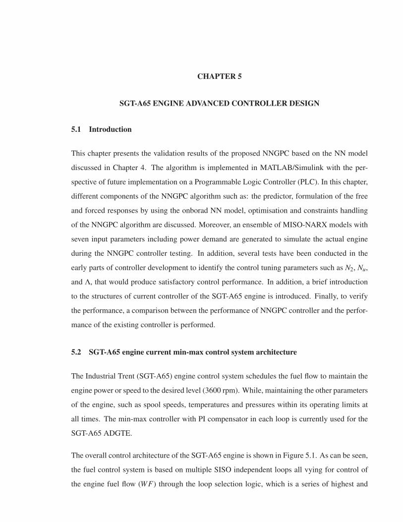
CHAPTER 5
SGT-A65 ENGINE ADVANCED CONTROLLER DESIGN
5.1 Introduction
This chapter presents the validation results of the proposed NNGPC based on the NN model
discussed in Chapter 4. The algorithm is implemented in MATLAB/Simulink with the per-
spective of future implementation on a Programmable Logic Controller (PLC). In this chapter,
different components of the NNGPC algorithm such as: the predictor, formulation of the free
and forced responses by using the onborad NN model, optimisation and constraints handling
of the NNGPC algorithm are discussed. Moreover, an ensemble of MISO-NARX models with
seven input parameters including power demand are generated to simulate the actual engine
during the NNGPC controller testing. In addition, several tests have been conducted in the
early parts of controller development to identify the control tuning parameters such as N2, Nu,
and Λ, that would produce satisfactory control performance. In addition, a brief introduction
to the structures of current controller of the SGT-A65 engine is introduced. Finally, to verify
the performance, a comparison between the performance of NNGPC controller and the perfor-
mance of the existing controller is performed.
5.2 SGT-A65 engine current min-max control system architecture
The Industrial Trent (SGT-A65) engine control system schedules the fuel flow to maintain the
engine power or speed to the desired level (3600 rpm). While, maintaining the other parameters
of the engine, such as spool speeds, temperatures and pressures within its operating limits at
all times. The min-max controller with PI compensator in each loop is currently used for the
SGT-A65 ADGTE.
The overall control architecture of the SGT-A65 engine is shown in Figure 5.1. As can be seen,
the fuel control system is based on multiple SISO independent loops all vying for control of
the engine fuel flow (WF) through the loop selection logic, which is a series of highest and
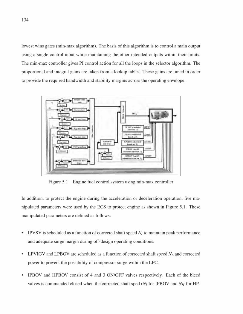
134
lowest wins gates (min-max algorithm). The basis of this algorithm is to control a main output
using a single control input while maintaining the other intended outputs within their limits.
The min-max controller gives PI control action for all the loops in the selector algorithm. The
proportional and integral gains are taken from a lookup tables. These gains are tuned in order
to provide the required bandwidth and stability margins across the operating envelope.
Figure 5.1 Engine fuel control system using min-max controller
In addition, to protect the engine during the acceleration or deceleration operation, five ma-
nipulated parameters were used by the ECS to protect engine as shown in Figure 5.1. These
manipulated parameters are defined as follows:
• IPVSV is scheduled as a function of corrected shaft speed NI to maintain peak performance
and adequate surge margin during off-design operating conditions.
• LPVIGV and LPBOV are scheduled as a function of corrected shaft speed NL and corrected
power to prevent the possibility of compressor surge within the LPC.
• IPBOV and HPBOV consist of 4 and 3 ON/OFF valves respectively. Each of the bleed
valves is commanded closed when the corrected shaft sped (NI for IPBOV and NH for HP-
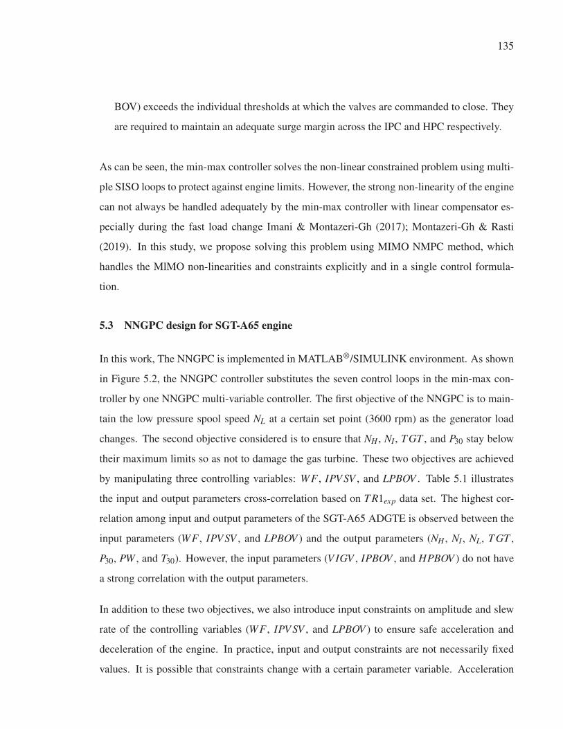
135
BOV) exceeds the individual thresholds at which the valves are commanded to close. They
are required to maintain an adequate surge margin across the IPC and HPC respectively.
As can be seen, the min-max controller solves the non-linear constrained problem using multi-
ple SISO loops to protect against engine limits. However, the strong non-linearity of the engine
can not always be handled adequately by the min-max controller with linear compensator es-
pecially during the fast load change Imani & Montazeri-Gh (2017); Montazeri-Gh & Rasti
(2019). In this study, we propose solving this problem using MIMO NMPC method, which
handles the MlMO non-linearities and constraints explicitly and in a single control formula-
tion.
5.3 NNGPC design for SGT-A65 engine
In this work, The NNGPC is implemented in MATLAB®/SIMULINK environment. As shown
in Figure 5.2, the NNGPC controller substitutes the seven control loops in the min-max con-
troller by one NNGPC multi-variable controller. The first objective of the NNGPC is to main-
tain the low pressure spool speed NL at a certain set point (3600 rpm) as the generator load
changes. The second objective considered is to ensure that NH , NI , T GT , and P30 stay below
their maximum limits so as not to damage the gas turbine. These two objectives are achieved
by manipulating three controlling variables: WF , IPV SV , and LPBOV . Table 5.1 illustrates
the input and output parameters cross-correlation based on T R1exp data set. The highest cor-
relation among input and output parameters of the SGT-A65 ADGTE is observed between the
input parameters (WF , IPV SV , and LPBOV ) and the output parameters (NH , NI , NL, T GT ,
P30, PW , and T30). However, the input parameters (V IGV , IPBOV , and HPBOV ) do not have
a strong correlation with the output parameters.
In addition to these two objectives, we also introduce input constraints on amplitude and slew
rate of the controlling variables (WF , IPV SV , and LPBOV ) to ensure safe acceleration and
deceleration of the engine. In practice, input and output constraints are not necessarily fixed
values. It is possible that constraints change with a certain parameter variable. Acceleration
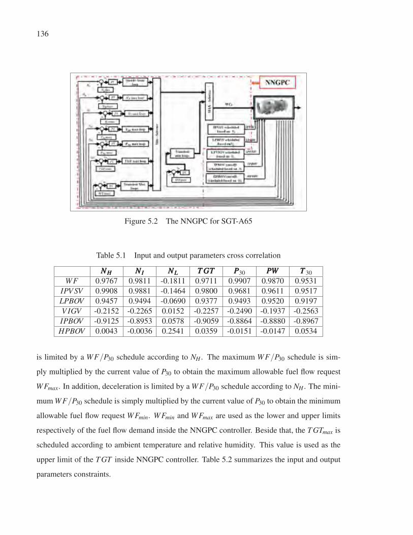
136
Figure 5.2 The NNGPC for SGT-A65
Table 5.1 Input and output parameters cross correlation
NNNHHH NNNIII NNNLLL TTT GGGTTT PPP30 PPPWWW TTT 30
WF 0.9767 0.9811 -0.1811 0.9711 0.9907 0.9870 0.9531
IPV SV 0.9908 0.9881 -0.1464 0.9800 0.9681 0.9611 0.9517
LPBOV 0.9457 0.9494 -0.0690 0.9377 0.9493 0.9520 0.9197
V IGV -0.2152 -0.2265 0.0152 -0.2257 -0.2490 -0.1937 -0.2563
IPBOV -0.9125 -0.8953 0.0578 -0.9059 -0.8864 -0.8880 -0.8967
HPBOV 0.0043 -0.0036 0.2541 0.0359 -0.0151 -0.0147 0.0534
is limited by a WF/P30 schedule according to NH . The maximum WF/P30 schedule is sim-
ply multiplied by the current value of P30 to obtain the maximum allowable fuel flow request
WFmax. In addition, deceleration is limited by a WF/P30 schedule according to NH . The mini-
mum WF/P30 schedule is simply multiplied by the current value of P30 to obtain the minimum
allowable fuel flow request WFmin. WFmin and WFmax are used as the lower and upper limits
respectively of the fuel flow demand inside the NNGPC controller. Beside that, the T GTmax is
scheduled according to ambient temperature and relative humidity. This value is used as the
upper limit of the T GT inside NNGPC controller. Table 5.2 summarizes the input and output
parameters constraints.
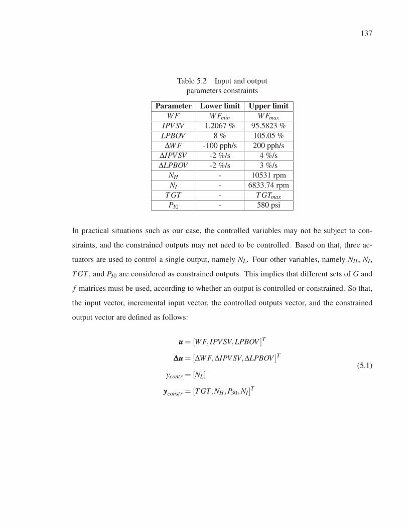
137
Table 5.2 Input and output
parameters constraints
Parameter Lower limit Upper limitWF WFmin WFmax
IPV SV 1.2067 % 95.5823 %
LPBOV 8 % 105.05 %
ΔWF -100 pph/s 200 pph/s
ΔIPV SV -2 %/s 4 %/s
ΔLPBOV -2 %/s 3 %/s
NH - 10531 rpm
NI - 6833.74 rpm
T GT - T GTmaxP30 - 580 psi
In practical situations such as our case, the controlled variables may not be subject to con-
straints, and the constrained outputs may not need to be controlled. Based on that, three ac-
tuators are used to control a single output, namely NL. Four other variables, namely NH , NI ,
T GT , and P30 are considered as constrained outputs. This implies that different sets of G and
f matrices must be used, according to whether an output is controlled or constrained. So that,
the input vector, incremental input vector, the controlled outputs vector, and the constrained
output vector are defined as follows:
uuu = [WF, IPV SV,LPBOV ]T
ΔΔΔuuu = [ΔWF,ΔIPV SV,ΔLPBOV ]T
ycontr = [NL]
yyyconstr = [T GT,NH ,P30,NI]T
(5.1)
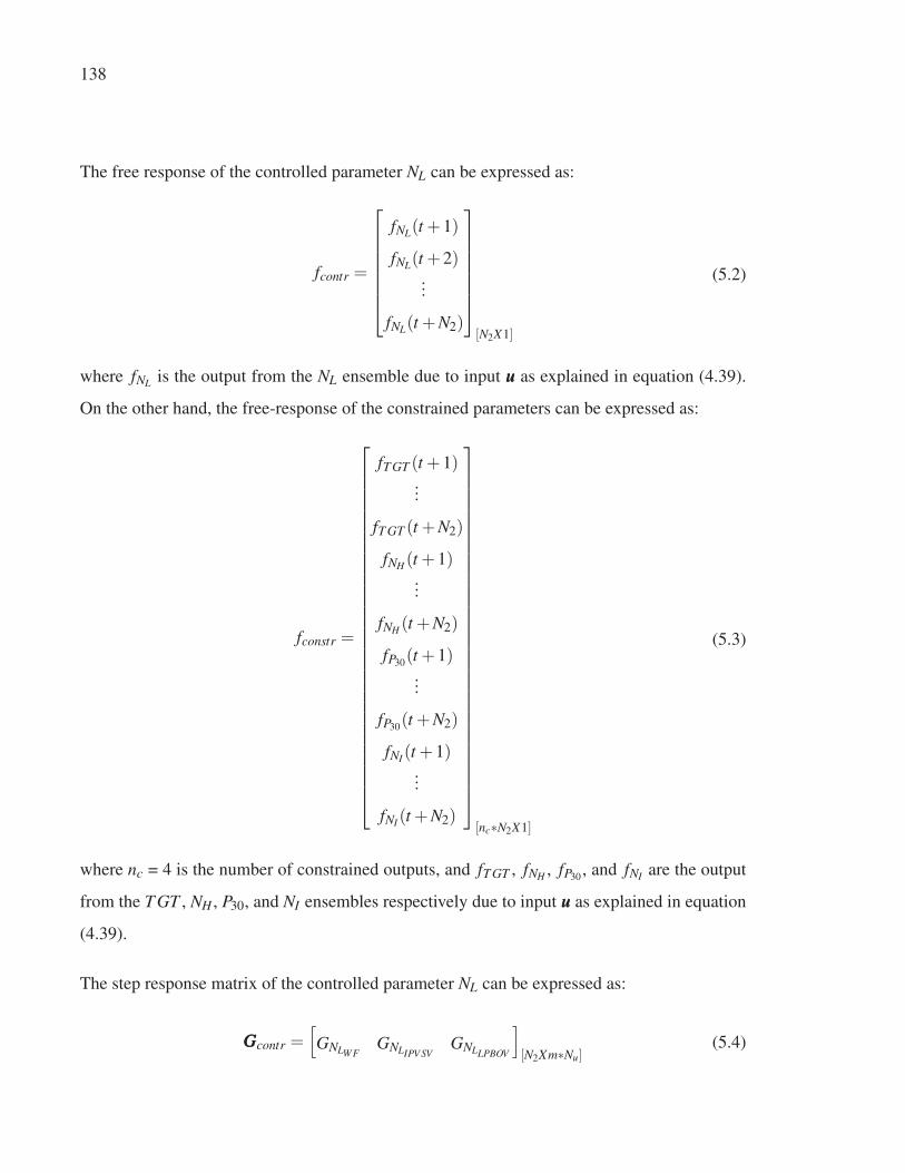
138
The free response of the controlled parameter NL can be expressed as:
fcontr =
⎡⎢⎢⎢⎢⎢⎢⎣
fNL(t +1)
fNL(t +2)...
fNL(t +N2)
⎤⎥⎥⎥⎥⎥⎥⎦[N2X1]
(5.2)
where fNL is the output from the NL ensemble due to input uuu as explained in equation (4.39).
On the other hand, the free-response of the constrained parameters can be expressed as:
fconstr =
⎡⎢⎢⎢⎢⎢⎢⎢⎢⎢⎢⎢⎢⎢⎢⎢⎢⎢⎢⎢⎢⎢⎢⎢⎢⎢⎢⎢⎢⎢⎢⎣
fT GT (t +1)...
fT GT (t +N2)
fNH (t +1)...
fNH (t +N2)
fP30(t +1)...
fP30(t +N2)
fNI(t +1)...
fNI(t +N2)
⎤⎥⎥⎥⎥⎥⎥⎥⎥⎥⎥⎥⎥⎥⎥⎥⎥⎥⎥⎥⎥⎥⎥⎥⎥⎥⎥⎥⎥⎥⎥⎦[nc∗N2X1]
(5.3)
where nc = 4 is the number of constrained outputs, and fT GT , fNH , fP30, and fNI are the output
from the T GT , NH , P30, and NI ensembles respectively due to input uuu as explained in equation
(4.39).
The step response matrix of the controlled parameter NL can be expressed as:
GGGcontr =[GNLWF
GNLIPV SVGNLLPBOV
][N2Xm∗Nu]
(5.4)
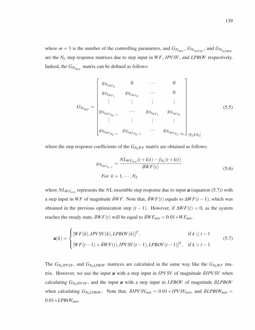
139
where m = 3 is the number of the controlling parameters, and GNLWF, GNLIPV SV
, and GNLLPBOV
are the NL step response matrices due to step input in WF , IPV SV , and LPBOV respectively.
Indeed, the GNLWFmatrix can be defined as follows:
GNLWF=
⎡⎢⎢⎢⎢⎢⎢⎢⎢⎢⎢⎢⎢⎢⎣
gNLWF00 · · · 0
gNLWF1gNLWF0
· · · 0
......
......
gNLWFNu−1· · · gNLWF1
gNLWF0
......
......
gNLWFN2−1gNLWFN2−2
· · · gNLWFN2−Nu
⎤⎥⎥⎥⎥⎥⎥⎥⎥⎥⎥⎥⎥⎥⎦[N2XNu]
(5.5)
where the step response coefficients of the GNLWF matrix are obtained as follows:
gNLWFk−1=
NLWFstep(t + k|t)− fNL(t + k|t)δWF(t)
For k = 1, · · · ,N2
(5.6)
where NLWFstep represents the NL ensemble step response due to input uuu (equation (5.7)) with
a step input in WF of magnitude δWF . Note that, δWF(t) equals to ΔWF(t −1), which was
obtained in the previous optimization step (t − 1). However, if ΔWF(t) = 0, as the system
reaches the steady state, δWF(t) will be equal to δWFmin = 0.01∗WFmin.
uuu(k) =
⎧⎪⎨⎪⎩[WF(k), IPV SV (k),LPBOV (k)]T , if k ≤ t −1
[WF(t −1)+δWF(t), IPV SV (t −1),LPBOV (t −1)]T , if k > t −1
(5.7)
The GNLIPV SV , and GNLLPBOV matrices are calculated in the same way like the GNLWF ma-
trix. However, we use the input uuu with a step input in IPV SV of magnitude δ IPV SV when
calculating GNLIPV SV , and the input uuu with a step input in LPBOV of magnitude δLPBOV
when calculating GNLLPBOV . Note that, δ IPV SVmin = 0.01 ∗ IPV SVmin, and δLPBOVmin =
0.01∗LPBOVmin.
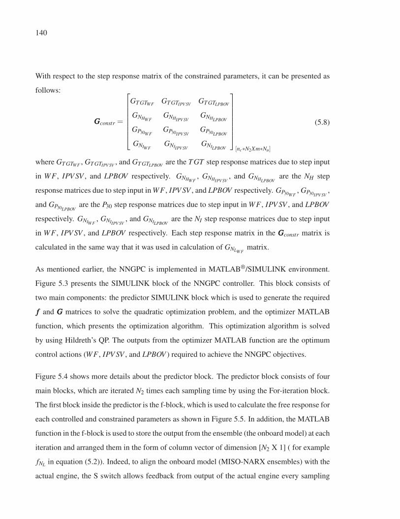
140
With respect to the step response matrix of the constrained parameters, it can be presented as
follows:
GGGconstr =
⎡⎢⎢⎢⎢⎢⎢⎣
GT GTWF GT GTIPV SV GT GTLPBOV
GNHWFGNHIPV SV
GNHLPBOV
GP30WFGP30IPV SV
GP30LPBOV
GNIWFGNIIPV SV
GNILPBOV
⎤⎥⎥⎥⎥⎥⎥⎦[nc∗N2Xm∗Nu]
(5.8)
where GT GTWF , GT GTIPV SV , and GT GTLPBOV are the T GT step response matrices due to step input
in WF , IPV SV , and LPBOV respectively. GNHWF, GNHIPV SV
, and GNHLPBOVare the NH step
response matrices due to step input in WF , IPV SV , and LPBOV respectively. GP30WF, GP30IPV SV
,
and GP30LPBOVare the P30 step response matrices due to step input in WF , IPV SV , and LPBOV
respectively. GNIWF, GNIIPV SV
, and GNILPBOVare the NI step response matrices due to step input
in WF , IPV SV , and LPBOV respectively. Each step response matrix in the GGGconstr matrix is
calculated in the same way that it was used in calculation of GNLWFmatrix.
As mentioned earlier, the NNGPC is implemented in MATLAB®/SIMULINK environment.
Figure 5.3 presents the SIMULINK block of the NNGPC controller. This block consists of
two main components: the predictor SIMULINK block which is used to generate the required
fff and GGG matrices to solve the quadratic optimization problem, and the optimizer MATLAB
function, which presents the optimization algorithm. This optimization algorithm is solved
by using Hildreth’s QP. The outputs from the optimizer MATLAB function are the optimum
control actions (WF , IPV SV , and LPBOV ) required to achieve the NNGPC objectives.
Figure 5.4 shows more details about the predictor block. The predictor block consists of four
main blocks, which are iterated N2 times each sampling time by using the For-iteration block.
The first block inside the predictor is the f-block, which is used to calculate the free response for
each controlled and constrained parameters as shown in Figure 5.5. In addition, the MATLAB
function in the f-block is used to store the output from the ensemble (the onboard model) at each
iteration and arranged them in the form of column vector of dimension [N2 X 1] ( for example
fNL in equation (5.2)). Indeed, to align the onboard model (MISO-NARX ensembles) with the
actual engine, the S switch allows feedback from output of the actual engine every sampling
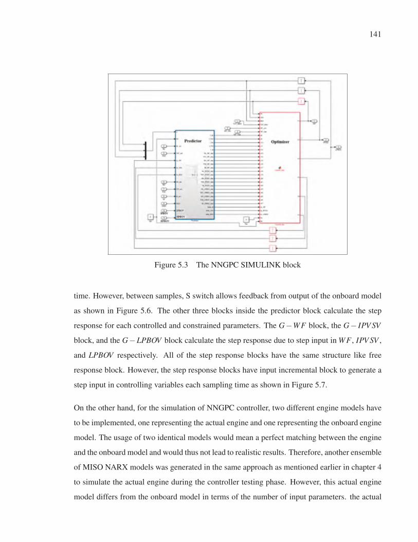
141
Figure 5.3 The NNGPC SIMULINK block
time. However, between samples, S switch allows feedback from output of the onboard model
as shown in Figure 5.6. The other three blocks inside the predictor block calculate the step
response for each controlled and constrained parameters. The G−WF block, the G− IPV SV
block, and the G−LPBOV block calculate the step response due to step input in WF , IPV SV ,
and LPBOV respectively. All of the step response blocks have the same structure like free
response block. However, the step response blocks have input incremental block to generate a
step input in controlling variables each sampling time as shown in Figure 5.7.
On the other hand, for the simulation of NNGPC controller, two different engine models have
to be implemented, one representing the actual engine and one representing the onboard engine
model. The usage of two identical models would mean a perfect matching between the engine
and the onboard model and would thus not lead to realistic results. Therefore, another ensemble
of MISO NARX models was generated in the same approach as mentioned earlier in chapter 4
to simulate the actual engine during the controller testing phase. However, this actual engine
model differs from the onboard model in terms of the number of input parameters. the actual
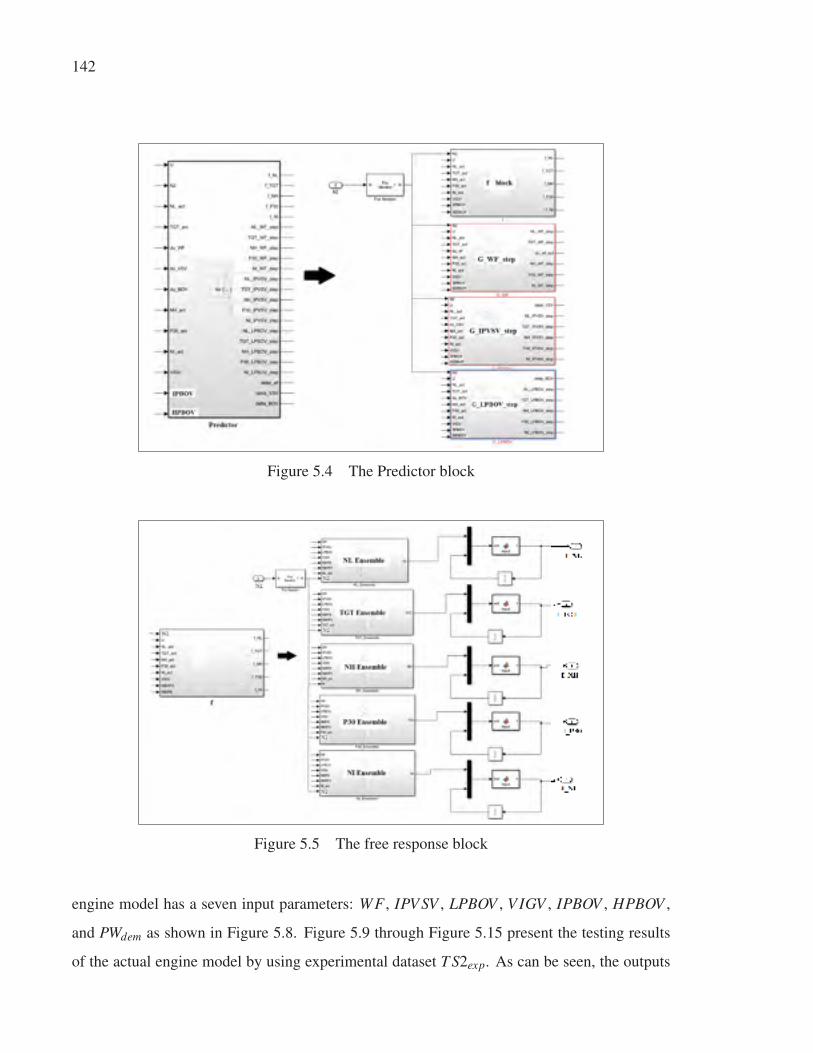
142
Figure 5.4 The Predictor block
Figure 5.5 The free response block
engine model has a seven input parameters: WF , IPV SV , LPBOV , V IGV , IPBOV , HPBOV ,
and PWdem as shown in Figure 5.8. Figure 5.9 through Figure 5.15 present the testing results
of the actual engine model by using experimental dataset T S2exp. As can be seen, the outputs
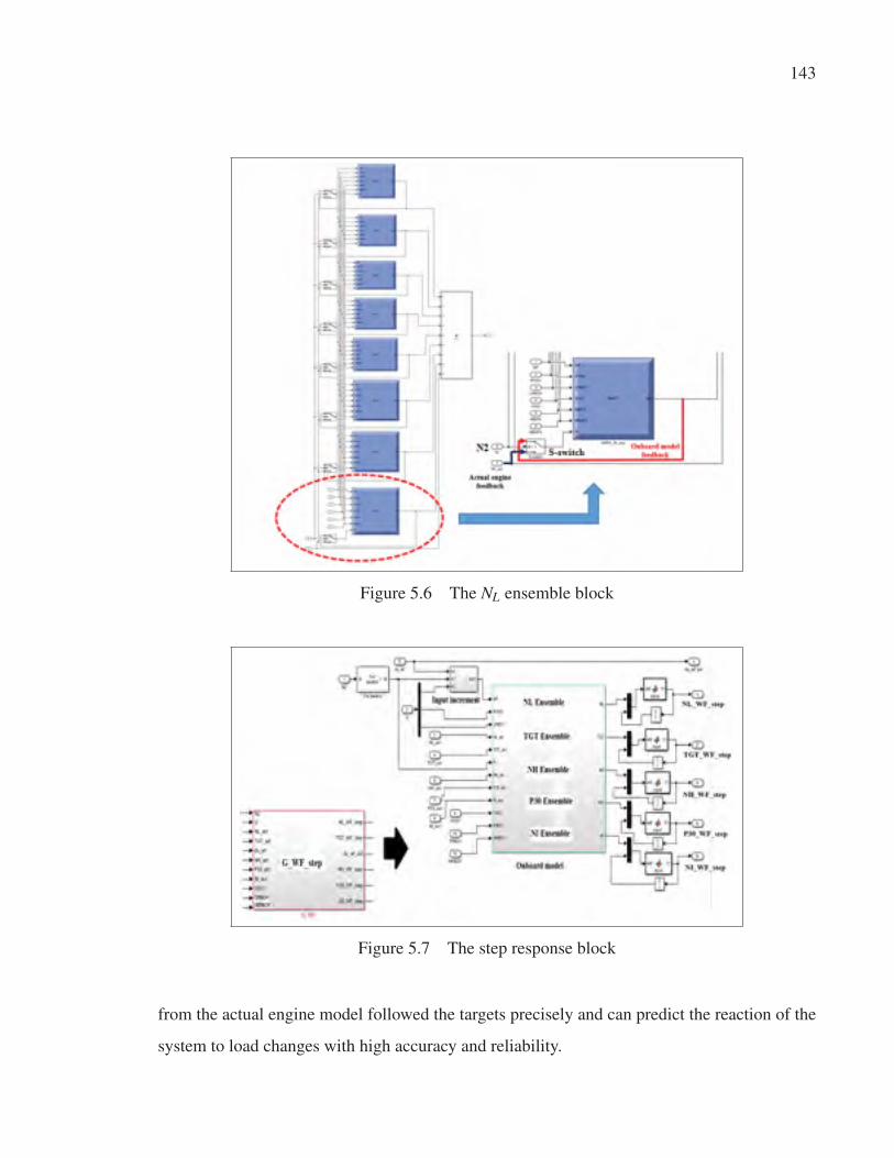
143
Figure 5.6 The NL ensemble block
Figure 5.7 The step response block
from the actual engine model followed the targets precisely and can predict the reaction of the
system to load changes with high accuracy and reliability.
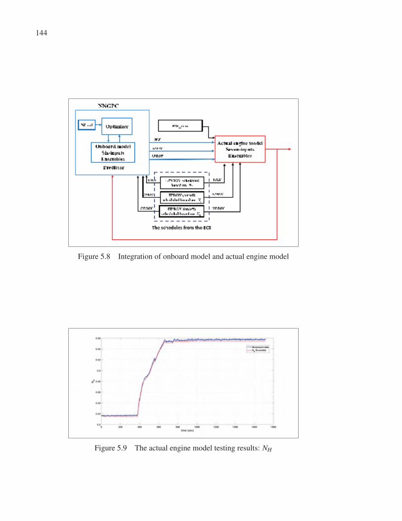
144
Figure 5.8 Integration of onboard model and actual engine model
Figure 5.9 The actual engine model testing results: NH
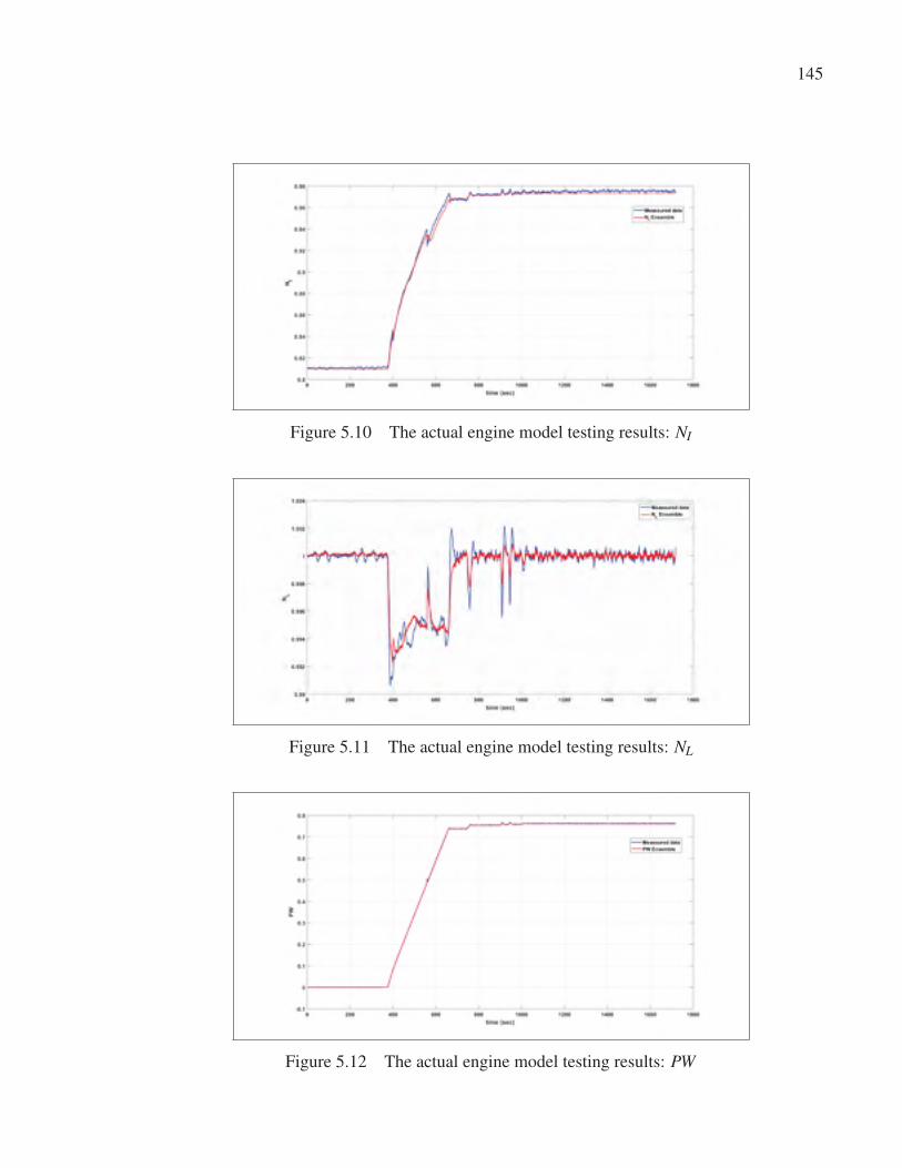
145
Figure 5.10 The actual engine model testing results: NI
Figure 5.11 The actual engine model testing results: NL
Figure 5.12 The actual engine model testing results: PW
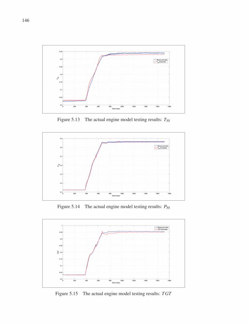
146
Figure 5.13 The actual engine model testing results: T30
Figure 5.14 The actual engine model testing results: P30
Figure 5.15 The actual engine model testing results: T GT
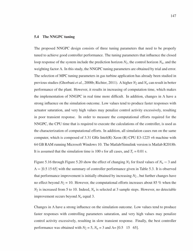
147
5.4 The NNGPC tuning
The proposed NNGPC design consists of three tuning parameters that need to be properly
tuned to achieve good controller performance. The tuning parameters that influence the closed
loop response of the system include the prediction horizon N2, the control horizon Nu, and the
weighting factor Λ. In this study, the NNGPC tuning parameters are obtained by trial and error.
The selection of MPC tuning parameters in gas turbine application has already been studied in
previous studies (Ghorbani et al., 2008b; Richter, 2011). A higher N2 and Nu can result in better
performance of the plant. However, it results in increasing of computation time, which makes
the implementation of NNGPC in real time more difficult. In addition, changes in Λ have a
strong influence on the simulation outcome. Low values tend to produce faster responses with
actuator saturation, and very high values may penalize control activity excessively, resulting
in poor transient response. In order to measure the computational efforts required for the
NNGPC, the CPU time that is required to execute the calculations of the controller, is used as
the characterization of computational efforts. In addition, all simulation cases run on the same
computer, which is composed of 3.31 GHz Intel(R) Xeon (R) CPU E3-1225 v6 machine with
64 GB RAM running Microsoft Windows 10. The Matlab/Simulink version is Matlab R2018b.
It is assumed that the simulation time is 100 s for all cases, and Ts = 0.01 s.
Figure 5.16 through Figure 5.20 show the effect of changing N2 for fixed values of Nu = 3 and
Λ = [0.5 15 65] with the summary of controller performance given in Table 5.3. It is observed
that performance improvement is initially obtained by increasing N2 , but further changes have
no effect beyond N2 = 10. However, the computational efforts increases about 85 % when the
N2 is increased from 5 to 10. Indeed, Nu is selected at 3 sample steps. However, no detectable
improvement occurs beyond Nu equal 3.
Changes in Λ have a strong influence on the simulation outcome. Low values tend to produce
faster responses with controlling parameters saturation, and very high values may penalize
control activity excessively, resulting in slow transient response. Finally, the best controller
performance was obtained with N2 = 5, Nu = 3 and Λ= [0.5 15 65].
148
Table 5.3 The control performance comparison with various N2 values
Output parameter NNN222 Settling time (s) Overshoot (%) Computation time (s)
PW3 18.63 4.1 15.39
5 7.6 4 35.34
10 7.5 15.7 245.68
NL
3 10.27 9.4 15.39
5 3.7 4 35.34
10 3.61 3.8 245.68
Figure 5.16 Effect of prediction horizon on PW
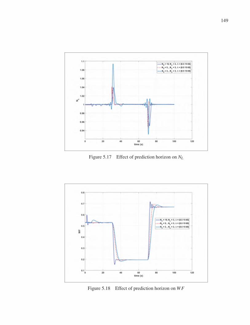
149
Figure 5.17 Effect of prediction horizon on NL
Figure 5.18 Effect of prediction horizon on WF
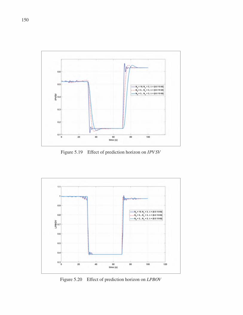
150
Figure 5.19 Effect of prediction horizon on IPV SV
Figure 5.20 Effect of prediction horizon on LPBOV
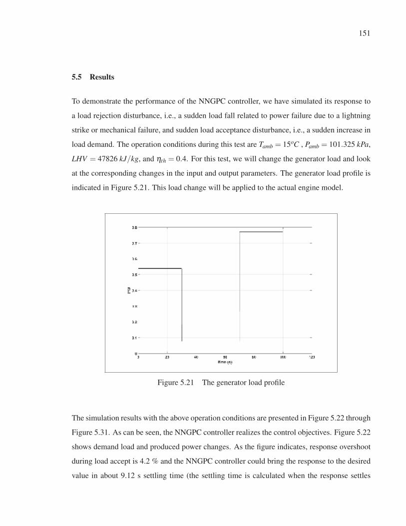
151
5.5 Results
To demonstrate the performance of the NNGPC controller, we have simulated its response to
a load rejection disturbance, i.e., a sudden load fall related to power failure due to a lightning
strike or mechanical failure, and sudden load acceptance disturbance, i.e., a sudden increase in
load demand. The operation conditions during this test are Tamb = 15oC , Pamb = 101.325 kPa,
LHV = 47826 kJ/kg, and ηth = 0.4. For this test, we will change the generator load and look
at the corresponding changes in the input and output parameters. The generator load profile is
indicated in Figure 5.21. This load change will be applied to the actual engine model.
Figure 5.21 The generator load profile
The simulation results with the above operation conditions are presented in Figure 5.22 through
Figure 5.31. As can be seen, the NNGPC controller realizes the control objectives. Figure 5.22
shows demand load and produced power changes. As the figure indicates, response overshoot
during load accept is 4.2 % and the NNGPC controller could bring the response to the desired
value in about 9.12 s settling time (the settling time is calculated when the response settles
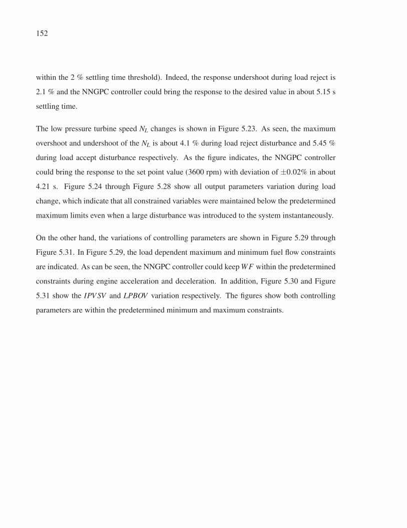
152
within the 2 % settling time threshold). Indeed, the response undershoot during load reject is
2.1 % and the NNGPC controller could bring the response to the desired value in about 5.15 s
settling time.
The low pressure turbine speed NL changes is shown in Figure 5.23. As seen, the maximum
overshoot and undershoot of the NL is about 4.1 % during load reject disturbance and 5.45 %
during load accept disturbance respectively. As the figure indicates, the NNGPC controller
could bring the response to the set point value (3600 rpm) with deviation of ±0.02% in about
4.21 s. Figure 5.24 through Figure 5.28 show all output parameters variation during load
change, which indicate that all constrained variables were maintained below the predetermined
maximum limits even when a large disturbance was introduced to the system instantaneously.
On the other hand, the variations of controlling parameters are shown in Figure 5.29 through
Figure 5.31. In Figure 5.29, the load dependent maximum and minimum fuel flow constraints
are indicated. As can be seen, the NNGPC controller could keep WF within the predetermined
constraints during engine acceleration and deceleration. In addition, Figure 5.30 and Figure
5.31 show the IPV SV and LPBOV variation respectively. The figures show both controlling
parameters are within the predetermined minimum and maximum constraints.
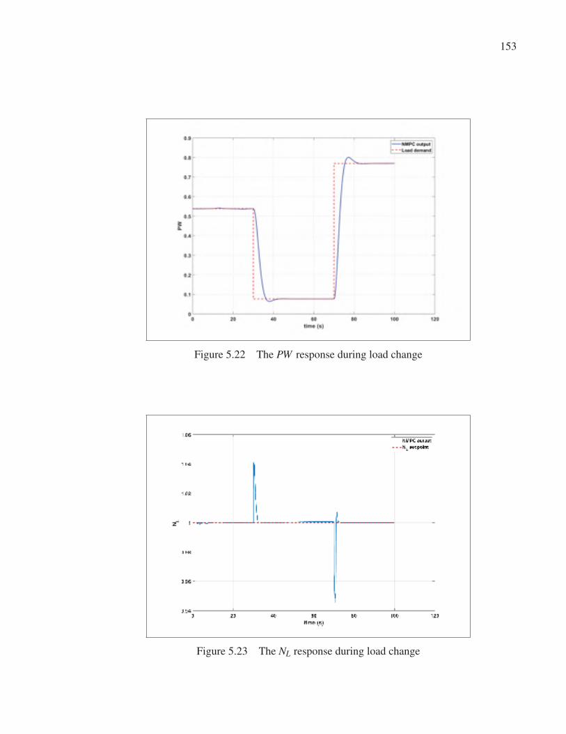
153
Figure 5.22 The PW response during load change
Figure 5.23 The NL response during load change
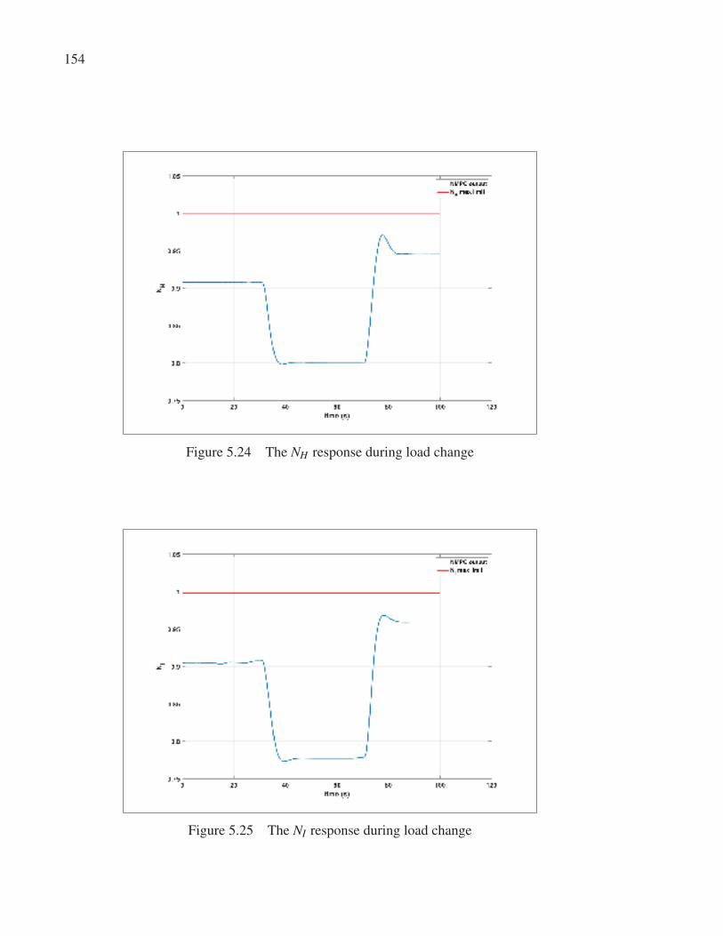
154
Figure 5.24 The NH response during load change
Figure 5.25 The NI response during load change
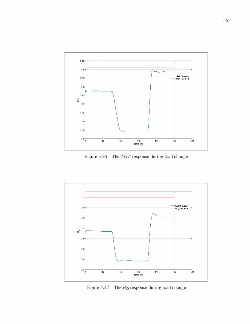
155
Figure 5.26 The T GT response during load change
Figure 5.27 The P30 response during load change
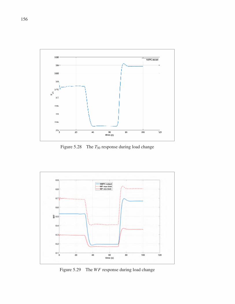
156
Figure 5.28 The T30 response during load change
Figure 5.29 The WF response during load change
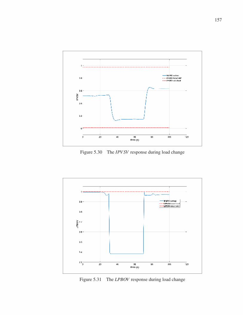
157
Figure 5.30 The IPV SV response during load change
Figure 5.31 The LPBOV response during load change
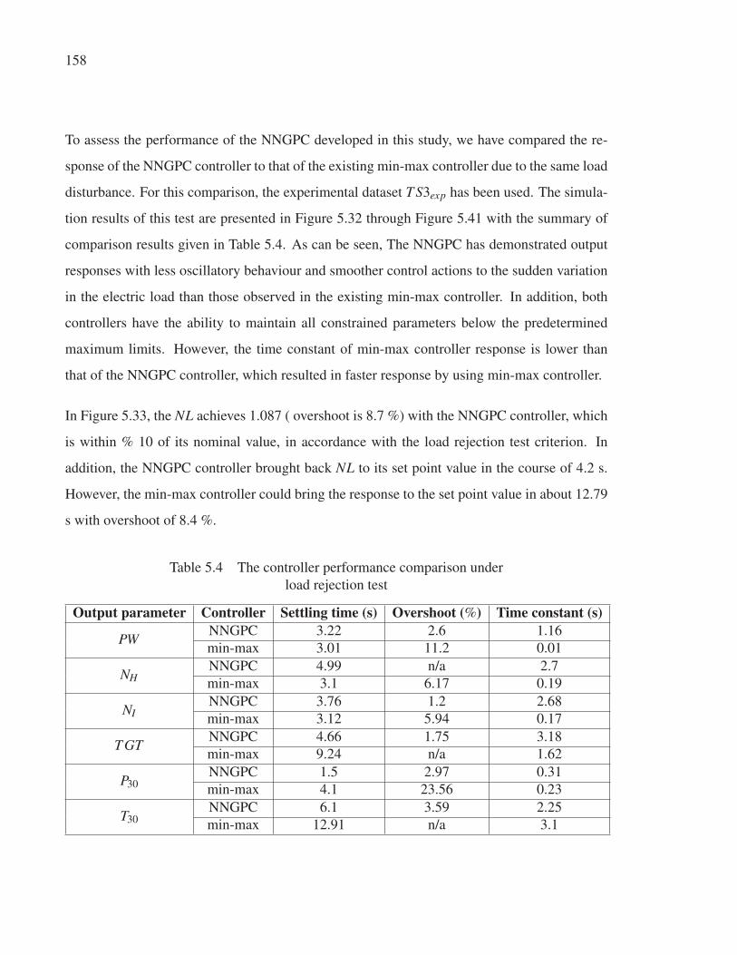
158
To assess the performance of the NNGPC developed in this study, we have compared the re-
sponse of the NNGPC controller to that of the existing min-max controller due to the same load
disturbance. For this comparison, the experimental dataset T S3exp has been used. The simula-
tion results of this test are presented in Figure 5.32 through Figure 5.41 with the summary of
comparison results given in Table 5.4. As can be seen, The NNGPC has demonstrated output
responses with less oscillatory behaviour and smoother control actions to the sudden variation
in the electric load than those observed in the existing min-max controller. In addition, both
controllers have the ability to maintain all constrained parameters below the predetermined
maximum limits. However, the time constant of min-max controller response is lower than
that of the NNGPC controller, which resulted in faster response by using min-max controller.
In Figure 5.33, the NL achieves 1.087 ( overshoot is 8.7 %) with the NNGPC controller, which
is within % 10 of its nominal value, in accordance with the load rejection test criterion. In
addition, the NNGPC controller brought back NL to its set point value in the course of 4.2 s.
However, the min-max controller could bring the response to the set point value in about 12.79
s with overshoot of 8.4 %.
Table 5.4 The controller performance comparison under
load rejection test
Output parameter Controller Settling time (s) Overshoot (%) Time constant (s)
PWNNGPC 3.22 2.6 1.16
min-max 3.01 11.2 0.01
NHNNGPC 4.99 n/a 2.7
min-max 3.1 6.17 0.19
NINNGPC 3.76 1.2 2.68
min-max 3.12 5.94 0.17
T GTNNGPC 4.66 1.75 3.18
min-max 9.24 n/a 1.62
P30NNGPC 1.5 2.97 0.31
min-max 4.1 23.56 0.23
T30NNGPC 6.1 3.59 2.25
min-max 12.91 n/a 3.1
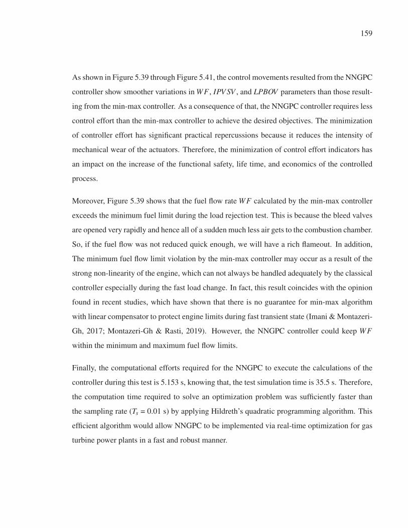
159
As shown in Figure 5.39 through Figure 5.41, the control movements resulted from the NNGPC
controller show smoother variations in WF , IPV SV , and LPBOV parameters than those result-
ing from the min-max controller. As a consequence of that, the NNGPC controller requires less
control effort than the min-max controller to achieve the desired objectives. The minimization
of controller effort has significant practical repercussions because it reduces the intensity of
mechanical wear of the actuators. Therefore, the minimization of control effort indicators has
an impact on the increase of the functional safety, life time, and economics of the controlled
process.
Moreover, Figure 5.39 shows that the fuel flow rate WF calculated by the min-max controller
exceeds the minimum fuel limit during the load rejection test. This is because the bleed valves
are opened very rapidly and hence all of a sudden much less air gets to the combustion chamber.
So, if the fuel flow was not reduced quick enough, we will have a rich flameout. In addition,
The minimum fuel flow limit violation by the min-max controller may occur as a result of the
strong non-linearity of the engine, which can not always be handled adequately by the classical
controller especially during the fast load change. In fact, this result coincides with the opinion
found in recent studies, which have shown that there is no guarantee for min-max algorithm
with linear compensator to protect engine limits during fast transient state (Imani & Montazeri-
Gh, 2017; Montazeri-Gh & Rasti, 2019). However, the NNGPC controller could keep WF
within the minimum and maximum fuel flow limits.
Finally, the computational efforts required for the NNGPC to execute the calculations of the
controller during this test is 5.153 s, knowing that, the test simulation time is 35.5 s. Therefore,
the computation time required to solve an optimization problem was sufficiently faster than
the sampling rate (Ts = 0.01 s) by applying Hildreth’s quadratic programming algorithm. This
efficient algorithm would allow NNGPC to be implemented via real-time optimization for gas
turbine power plants in a fast and robust manner.
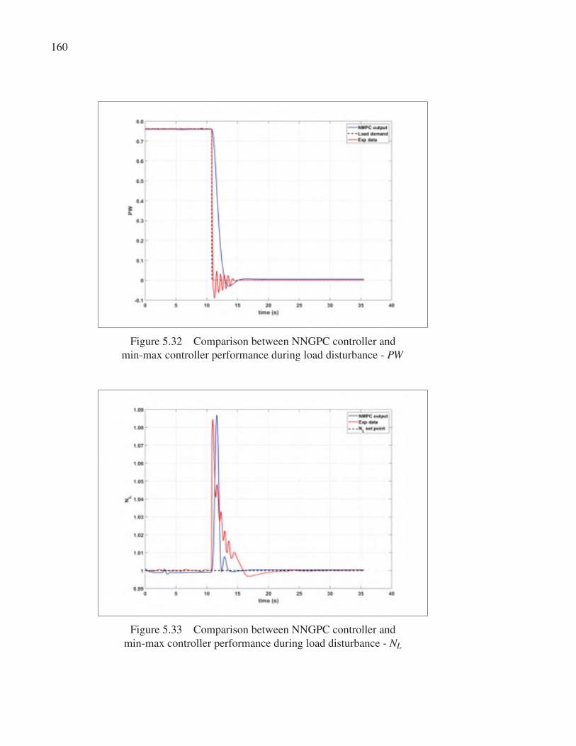
160
Figure 5.32 Comparison between NNGPC controller and
min-max controller performance during load disturbance - PW
Figure 5.33 Comparison between NNGPC controller and
min-max controller performance during load disturbance - NL
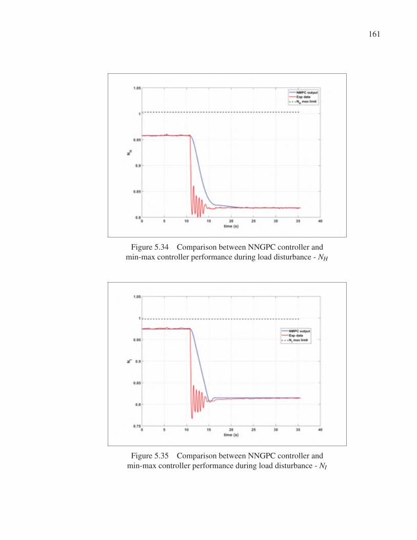
161
Figure 5.34 Comparison between NNGPC controller and
min-max controller performance during load disturbance - NH
Figure 5.35 Comparison between NNGPC controller and
min-max controller performance during load disturbance - NI
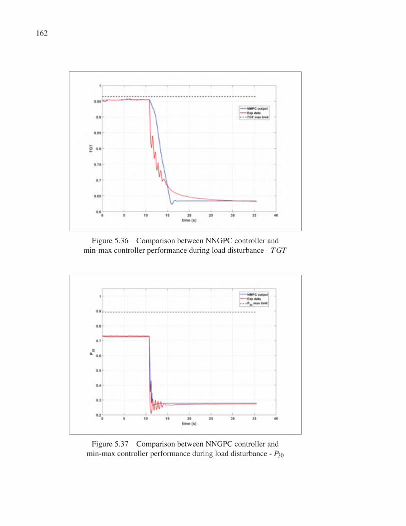
162
Figure 5.36 Comparison between NNGPC controller and
min-max controller performance during load disturbance - T GT
Figure 5.37 Comparison between NNGPC controller and
min-max controller performance during load disturbance - P30
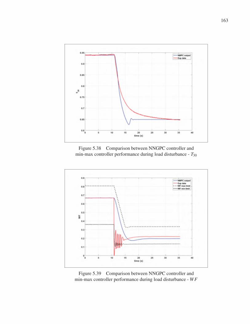
163
Figure 5.38 Comparison between NNGPC controller and
min-max controller performance during load disturbance - T30
Figure 5.39 Comparison between NNGPC controller and
min-max controller performance during load disturbance - WF
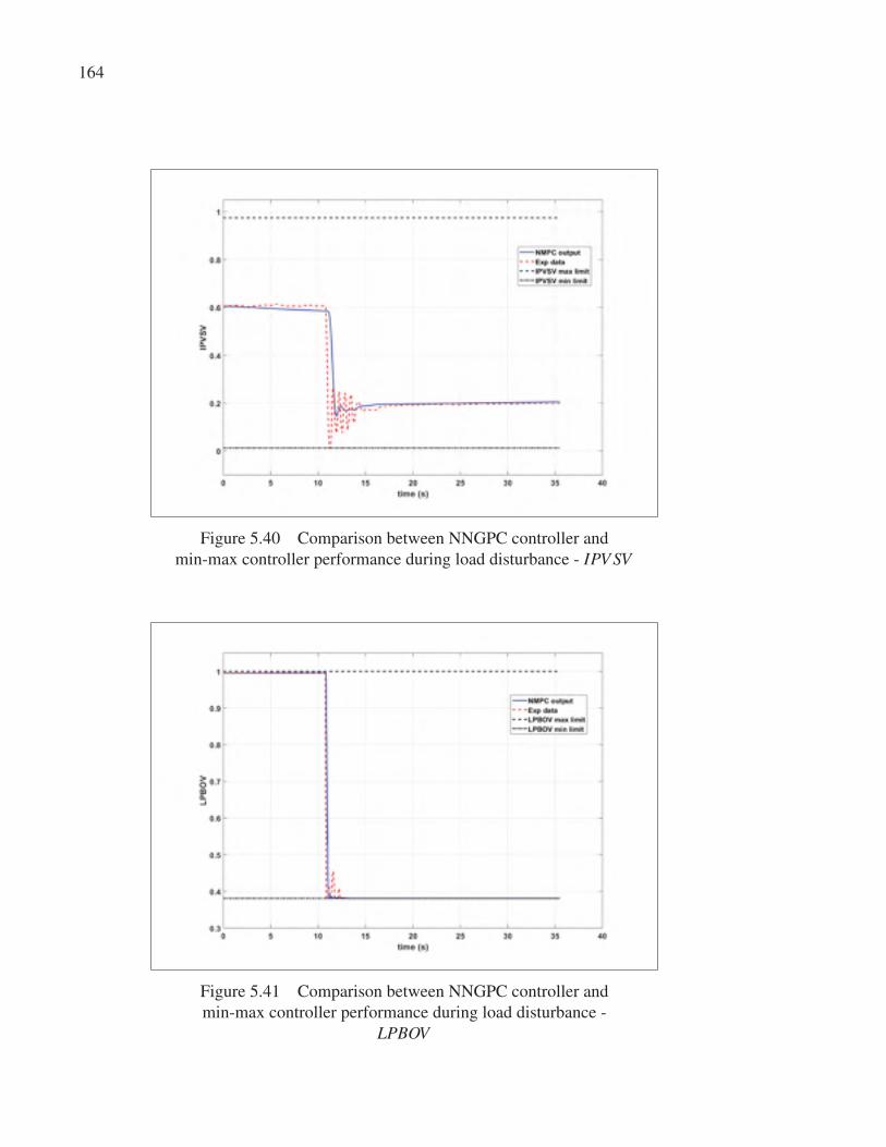
164
Figure 5.40 Comparison between NNGPC controller and
min-max controller performance during load disturbance - IPV SV
Figure 5.41 Comparison between NNGPC controller and
min-max controller performance during load disturbance -
LPBOV
165
5.6 Summary
The simulation results for the SGT-A65 engine controlled by the NNGPC controller was pre-
sented in this chapter. As can be seen, the simulation results show that although NNGPC can
not produce faster response, in terms of time constant, than min-max controller, it resulted in
less oscillatory behaviour and smoother control actions to the sudden variation in the electric
load than those observed in the existing min-max controller. In addition, computation time
required to solve an optimization problem was sufficiently faster than the sampling rate that al-
low a real time implementation of the NNGPC controller. Moreover, the use of controllers that
take into account the non-linearities of the plant implies an improvement in the performance of
the plant by reducing the impact of the disturbances and by improving the tracking capabilities
of the control system.
In addition, a larger prediction horizon can make a faster response and better control qual-
ity. However, it will also greatly increase the calculation and affect real time performance of
NNGPC controller. So that, as an indication of forthcoming research, it is intended to use an
optimization approach to perform NMPC tuning and find the best tuning parameters based on
the desired performance characteristics.

CONCLUSIONS AND RECOMMENDATIONS
6.1 Conclusions
This thesis focuses on solving important challenges in the area of gas turbine engine’s con-
troller design to ensure the safe operation of the engine and at the same time get the maxi-
mum performance. The system identification and advanced control algorithms based on NN
methodology were developed to control an ADGTE used in power generation application under
loading and unloading condition. The main results can be summarized as follows;
1. A novel methodology for the development of real time data driven based model of ADGTE
was presented in Chapter 3 to address the first objective. An ensemble of multiple MISO-
NARX neural models was introduced to predict the ADGTE output parameters in real time.
Inspired by the way biological neural networks process information and by their structure
which changes depending on their function, multiple-input single-output (MISO) NARX
models with different configurations were used to represent each of the ADGTE output
parameters with the same input parameters.
2. Estimation of the NN model order by generating different ARX models and estimation of
the input/output delay, before generation of NN model, are very important steps. These
steps save more iterations required to find the best structure of the NN and consequently
saving more time required for NN model generation. In addition, data cleaning and resam-
pling step significantly reduced training time. The lower sampling rate reduces the number
of data points, which reduces the computation time during training operation and reduces
data collinearity.
3. Usage of a single neural network to represent each of the system output parameters may not
be able to provide an accurate prediction for unseen data and as a consequence, provides
poor generalization. To overcome this problem, an ensemble of MISO NARX models was

168
used to represent each output parameter. The major challenge of the ensemble generation
is to decide how to combine results produced by the ensemble’s components. A novel
hybrid dynamic weighting method (HDWM) was proposed to perform this task.
4. A comparison between the ensemble of MISO NARX models and the single MISO NARX
models for all engine output parameters at different operation conditions showed that, the
ensemble of MISO-NARX models can represent the ADGTE during the full operating
range with a good accuracy even with different input scenarios from different operation
conditions which prove the high generalization characteristic of the ensemble. Also, an-
other important gain was the very low execution time (40.5 μs), which can support many
real time applications like model based controller design, sensor fault verification and en-
gine health monitoring. Moreover, one can observe that the ensemble model demonstrates
a significantly better performance in identification of the gas turbine engine dynamics than
the individual neural model, as it resulted in an improvement in accuracy of nearly 90%,
compared with the single neural model.
5. With the desire to have more robustness and flexibility of the next generation of the GTE
control systems to achieve ambitious targets and severe limitations set by governments and
organizations, Chapter 4 outlined the NMPC controller design problem.
6. One of the key features of the NNGPC algorithm is the novel approach used to estimate the
free and forced responses of the GPC algorithm based on NN model. It reduces the NMPC
based optimization problem to a linear optimization problem at each sampling step. That
will improve the computation time and reliability of the solution.
7. In addition, a significantly important part of the constrained NNGPC controller is the nu-
merical optimization algorithm. The Hildreth’s QP procedure was utilized which offers
simplicity and reliability in real-time implementation (Wang, 2009). Furthermore, Hil-
169
dreth’s method may be useful to implement on non-PC platforms like programmable logic
controllers or embedded machine which do not support linear algebra libraries.
8. A comparison between the performance of NNGPC controller and the performance of the
existing min-max controller was performed. The NNGPC has demonstrated superior out-
put responses with less oscillatory behaviour and smoother control actions to the sudden
variation in the electric load than those observed in the existing min-max controller. In ad-
dition, computation time required to solve an optimization problem was sufficiently faster
than the sampling rate that allow a real time implementation of the NNGPC controller.
6.2 Recommendations
Some recommendations for further studies are outlined below:
1. As the only available experimental data from the real engine testing was collected at a
specific operation conditions, future work will involve looking at the NNGPC controller
performance over a different operation conditions and different transient scenarios and de-
termining what modifications are required to obtain acceptable robust performance. Once
the control algorithm is proven, we will focus on implementing the controllers we show-
cased here on Programmable Logic Controller (PLC) with the aim of eventually being
able to test it in a real life test bed environment. This process will involve converting the
NNGPC algorithm to structured text for implementation on a PLC.
2. In this thesis we studied the homogeneous ensemble models, where source of diversity was
the variation in the training data. An alternative would be studying heterogeneous ensem-
ble in which ensemble members have different architectures such as number of neurons,
number of layers, and training algorithm.

170
3. In this thesis, off-line learning techniques are applied for identifying the GTE dynamics.
A potential future work is to study the on-line ensemble learning to identify the GTE
dynamics while the engine is operating.
4. In this thesis, the max number of iterations in the Hildreth’s QP procedure was fixed to
100 iterations. In addition, we used the Lagrange multipliers values to identify the active
and inactive constrains. An investigation would be needed to study the effect of iteration
number and the significance of the Lagrange multipliers values obtained in the proposed
approach on the convergence speed and solution stability.
5. In this thesis the tuning of the NNGPC controller was performed by using the trial and
error method. However, there is still a need for a more systematic approach to perform
MPC tuning and find the best tuning parameters based on the desired performance charac-
teristics. MPC tuning is usually performed ad-hoc based on some experience. Most of the
time, several simulation runs are performed to check if the chosen tuning parameters are
suitable. Automated tuning procedures using genetic algorithm can be applied to reduce
the manual operations.

LIST OF PUBLICATION
The contributions of this work have been presented in two journals and three conference pub-
lications. The complete list of publications associated with this research work is presented
below.
Journals
1. Ibrahem, I. A., Akhrif., O., Moustapha., H. & Staniszewski., M. (2020b). An ensemble
of recurrent neural networks for real time performance modelling of three-spool
aero-derivative gas turbine engine, Submitted for publication in the ASME Journal
of Engineering for Gas Turbines and Power; July 2020. ( Accepted)
This paper is summarized in Chapter 3. It presents a novel methodology for the
development of data driven based model of ADGTE.
2. Ibrahem, I. A., Akhrif., O., Moustapha., H. & Staniszewski., M. Nonlinear Generalized
Predictive Controller Based on Ensemble of NARX Models for Industrial Gas
Turbine Engine, Submitted for publication in the Elsevier Journal of Energy; July
2020. ( Under review)
This paper is summarized in Chapters 4 and 5. It presents a novel approach used
in the development of a constrained MIMO NMPC for an ADGTE used for power
generation.
Conferences
Published:
3. Ibrahem, I. A., Akhrif., O., Moustapha., H. & Staniszewski., M. (2019). Neural Net-
works Modelling of Aero-derivative Gas Turbine Engine: A Comparison Study.

172
Proceedings of the 16th International Conference on Informatics in Control, Au-
tomation and Robotics - Volume 1: ICINCO,, pp. 738-745.
This paper is summarized in Chapter 2. It represents a preliminary investigation
based on a literature survey of a data-driven based modelling approach, which is
needed to select the best type of neural network to represent the ADGTE during
the full operating range.
4. Ibrahem, I. A., Akhrif., O., Moustapha., H. & Staniszewski., M. (2020c). An ensemble
of recurrent neural networks for real time performance modelling of three-spool
aero-derivative gas turbine engine. ASME Turbo Expo 2020: Power for Land, Sea,
and Air.
This paper is summarized in Chapter 3. Based on the recommendation from the
third paper, a single MISO NARX neural model was introduced to predict the
ADGTE output parameters in real time. However, the single MISO NARX neural
model may not be able to provide accurate prediction when it operates outside the
field in which it was trained.
5. Ibrahem, I. A., Akhrif., O., Moustapha., H. & Staniszewski., M. (2020a). Real-time
modelling and Hardware in the loop simulation of an aero-derivative gas turbine
engine. Proceedings of Global Power and Propulsion Society.
This paper is summarized in Chapter 3. Based on the recommendation from the
forth paper, an ensemble of multiple MISO NARX neural models was introduced
to predict the ADGTE output parameters in real time.
BIBLIOGRAPHY
Administration, F. A. (2011). Airplane Flying Handbook (FAA-H-8083-3A). Skyhorse Pub-
lishing Inc.
Alves, V. A. O., de Godoy, R. J. C. & Garcia, C. (2013). Optimal time delay estimation for
System Identification. 2013 American Control Conference, pp. 95–100.
Aly, A. & Atia, I. (2012). Neural Modeling and Predictive Control of a Small Turbojet Engine
(SR-30). 10th International Energy Conversion Engineering Conference, pp. 4242.
Amozegar, M. & Khorasani, K. (2016). An ensemble of dynamic neural network identifiers
for fault detection and isolation of gas turbine engines. Neural Networks, 76, 106–121.
Asgari, H. (2014). Modelling, Simulation and control of gas turbines using artificial neural
networks.
Asgari, H. & Chen, X. (2015). Gas turbines modeling, simulation, and control: using artificialneural networks. CRC Press.
Asgari, H., Chen, X. & Sainudiin, R. (2013). Modelling and simulation of gas turbines.
International Journal of Modelling, Identification and Control, 20(3), 253–270.
Asgari, H., Venturini, M., Chen, X. & Sainudiin, R. (2014). Modeling and simulation of the
transient behavior of an industrial power plant gas turbine. Journal of Engineering forGas Turbines and Power, 136(6), 061601.
Bahlawan, H., Morini, M., Pinelli, M., Spina, P. R. & Venturini, M. (2017). Development of
Reliable NARX Models of Gas Turbine Cold, Warm and Hot Start-Up. ASME TurboExpo 2017: Turbomachinery Technical Conference and Exposition.
Ballin, M. G. (1988). A high fidelity real-time simulation of a small turboshaft engine.
Beale, M. H., Hagan, M. T. & Demuth, H. B. (2015). Neural Network Toolbox™ User’s
Guide.
Behera, S., Choubey, A., Kanani, C. S., Patel, Y. S., Misra, R. & Sillitti, A. (2019). Ensemble
trees learning based improved predictive maintenance using IIoT for turbofan engines.
Proceedings of the 34th ACM/SIGAPP Symposium on Applied Computing, pp. 842–850.
Bettocchi, R., Pinelli, M., Spina, P., Venturini, M. & Burgio, M. (2004). Set up of a robust
neural network for gas turbine simulation. ASME Turbo Expo 2004: Power for Land,Sea, and Air, pp. 543–551.
Bettocchi, R., Spina, P. R. & Fabbri, F. (1996). Dynamic modeling of single-shaft indus-
trial gas turbine. ASME 1996 International Gas Turbine and Aeroengine Congress andExhibition.
174
Brown, G., Wyatt, J., Harris, R. & Yao, X. (2005). Diversity creation methods: a survey and
categorisation. Information Fusion, 6(1), 5–20.
Brunell, B. J., Bitmead, R. R. & Connolly, A. J. (2002). Nonlinear model predictive control
of an aircraft gas turbine engine. Proceedings of the 41st IEEE Conference on Decisionand Control, 2002., 4, 4649–4651.
Camacho, E. F. & Alba, C. B. (2013). Model predictive control. Springer Science & Business
Media.
Camporeale, S., Fortunato, B. & Mastrovito, M. (2006). A modular code for real time dynamic
simulation of gas turbines in simulink.
CASTRO, E. (2018). Diagram Of How the Brain Works Elegant Gemütlich Diagram Brain
Parts and Functions Bilder Menschliche. Consulted at http://www.dreamdiving-resort.
com/diagram-of-how-the-brain-works.
Chen, Q., Huang, J., Pan, M. & Lu, F. (2019). A Novel Real-Time Mechanism Modeling
Approach for Turbofan Engine. Energies, 12(19), 3791.
Chipperfield, A. & Fleming, P. (1996). Multiobjective gas turbine engine controller design
using genetic algorithms. IEEE Transactions on Industrial Electronics, 43(5), 583–587.
Clarke, D. W., Mohtadi, C. & Tuffs, P. (1987a). Generalized predictive control—Part I. The
basic algorithm. Automatica, 23(2), 137–148.
Clarke, D. W., Mohtadi, C. & Tuffs, P. (1987b). Generalized predictive control—part II
extensions and interpretations. Automatica, 23(2), 149–160.
Clarke, D. & Mohtadi, C. (1987). Properties of generalized predictive control. IFAC Proceed-ings Volumes, 20(5), 65–76.
Crainic, C., Harvey, R. & Thompson, A. (1997). Real Time Thermodynamic Transient Model
for Three Spool Turboprop Engine. ASME 1997 International Gas Turbine and Aero-engine Congress and Exhibition.
Cybenko, G. (1989). Approximation by superpositions of a sigmoidal function. Mathematicsof control, signals and systems, 2(4), 303–314.
de Sousa, J. F., Moreira, J. M., Soares, C. M. & Jorge, A. (2012). Ensemble approaches for
regression: A survey.
Diehl, M., Ferreau, H. J. & Haverbeke, N. (2009). Efficient numerical methods for nonlinear
MPC and moving horizon estimation. In Nonlinear model predictive control (pp. 391–
417). Springer.
Duyar, A., Gu, Z. & Litt, J. S. (1995). A simplified dynamic model of the T700 turboshaft
engine. Journal of the American Helicopter Society, 40(4), 62–70.
175
Effiom, S. O., Abam, F. I. & Nwankwojike, B. N. (2017). Performance evaluation of
aeroderivative gas turbine models derived from a high bypass turbofan for industrial
power generation. Cogent Engineering, 4(1), 1301235.
Esfahani, M. A. & Montazeri, M. (2016). Designing and Optimizing Multi-Objective Turbofan
Engine Control Algorithm Using Min-Max Method. International Journal of ComputerScience and Information Security, 14(8), 1040.
Fawke, A. & Saravanamuttoo, H. (1971). Digital computer methods for prediction of gas
turbine dynamic response. SAE Transactions, 1805–1813.
Fletcher, A. H. (1963). The Avon aircraft engine and its industrial power applications. Pro-ceedings of the Institution of Mechanical Engineers, 177(1), 1068–1074.
Forhad, M. M. I. & Bloomberg, M. (2015). Drive Train Over-Speed Prediction for Gas Fuel
Based Gas Turbine Power Generation Units. Turbo Expo: Power for Land, Sea, and Air,
56758, V006T05A024.
Fuksman, I. & Sirica, S. (2012). Real-time execution of a high fidelity aero-thermodynamic
turbofan engine simulation. Journal of engineering for gas turbines and power, 134(5).
Gaudet, S. R. (2008). Development of a dynamic modeling and control system design method-ology for gas turbines. (Ph.D. thesis, Carleton University).
Gazzetta Junior, H., Bringhenti, C., Barbosa, J. R. & Tomita, J. T. (2017). Real-time gas turbine
model for performance simulations. Journal of Aerospace Technology and Management,9(3), 346–356.
Ghorbani, H., Ghaffari, A. & Rahnama, M. (2008a). Constrained model predictive control im-
plementation for a heavy-duty gas turbine power plant. WSEAS Transactions on Systemsand Control, 3(6), 507–516.
Ghorbani, H., Ghaffari, A. & Rahnama, M. (2008b). Multivariable model predictive control
for a gas turbine power plant. Proceedings of the 10th WSEAS International Conferenceon Automatic Control, Modelling & Simulation, pp. 275–281.
Gill, P. E., Murray, W. & Wright, M. H. (2019). Practical optimization. SIAM.
Gu, C.-w., Wang, H., Ji, X.-x. & Li, X.-s. (2016). Development and application of a
thermodynamic-cycle performance analysis method of a three-shaft gas turbine. En-ergy, 112, 307–321.
Gülen, S. C. (2019). Gas Turbines for Electric Power Generation. Cambridge University
Press.
Haaser, F. & Casper, R. (1991). Development of the LM 6000: the World’s Most Efficient
Simple Cycle Industrial Gas Turbine. Pmc. ASME COGEN 1991, 177–188.
176
H.I.H. Saravanamuttoo,G.F.C. Rogers, P. S. H. C. A. (2017). Gas Turbine The-ory (ed. 7). Pearson. Consulted at http://gen.lib.rus.ec/book/index.php?md5=
e522f34d4e94f04313d3074c1e7ef784.
Horlock, J. (1997). Aero-engine derivative gas turbines for power generation: thermodynamic
and economic perspectives. Journal of engineering for gas turbines and power, 119(1).
Ibrahem, I. A., Akhrif., O., Moustapha., H. & Staniszewski., M. Nonlinear Generalized Predic-
tive Controller Based on Ensemble of NARX Models for Industrial Gas Turbine Engine.
Ibrahem, I. A., Akhrif., O., Moustapha., H. & Staniszewski., M. (2019). Neural Networks
Modelling of Aero-derivative Gas Turbine Engine: A Comparison Study. Proceedings ofthe 16th International Conference on Informatics in Control, Automation and Robotics- Volume 1: ICINCO,, pp. 738-745.
Ibrahem, I. A., Akhrif., O., Moustapha., H. & Staniszewski., M. (2020a). Real-time modelling
and Hardware in the loop simulation of an aero-derivative gas turbine engine. Proceed-ings of Global Power and Propulsion Society.
Ibrahem, I. A., Akhrif., O., Moustapha., H. & Staniszewski., M. (2020b). An ensemble
of recurrent neural networks for real time performance modelling of three-spool aero-
derivative gas turbine engine.
Ibrahem, I. A., Akhrif., O., Moustapha., H. & Staniszewski., M. (2020c). An ensemble
of recurrent neural networks for real time performance modelling of three-spool aero-
derivative gas turbine engine. ASME Turbo Expo 2020: Power for Land, Sea, and Air.
Imani, A. & Montazeri-Gh, M. (2017). Improvement of Min–Max limit protection in aircraft
engine control: An LMI approach. Aerospace Science and Technology, 68, 214–222.
Jafari, S. & Nikolaidis, T. (2018). Turbojet Engine Industrial Min–Max Controller Performance
Improvement Using Fuzzy Norms. Electronics, 7(11), 314.
Jaw, L. & Mattingly, J. (2009). Aircraft Engine Controls. American Institute of Aeronautics
and Astronautics, Inc.
Khalili, R. & Karrari, M. (2017). Modeling and identification of an industrial gas turbine using
classical and non-classical approaches. Electrical Engineering (ICEE), 2017 IranianConference on, pp. 667–672.
Khan, K. (2018). Surprising Discovery of Genetic Mosaic in Brain. Consulted at http://
aboutislam.net/science/health/surprising-discovery-genetic-mosaic-brain/.
Kim, J., Song, T., Kim, T. & Ro, S. (2001). Model development and simulation of transient
behavior of heavy duty gas turbines. J. Eng. Gas Turbines Power, 123(3), 589–594.
Kim, J. S., Powell, K. M. & Edgar, T. F. (2013). Nonlinear model predictive control for a
heavy-duty gas turbine power plant. 2013 American control conference, pp. 2952–2957.
177
Kong, C., Ki, J. & Koh, K. (1999). Steady-State and Transient Performance Simulation of
a Turboshaft Engine with Free Power Turbine. ASME 1999 International Gas Turbineand Aeroengine Congress and Exhibition.
Krummrein, T., Henke, M. & Kutne, P. (2018). A highly flexible approach on the steady-state
analysis of innovative micro gas turbine cycles. Journal of Engineering for Gas Turbinesand Power, 140(12).
Kyprianidis, K. & Kalfas, A. I. (2008). Dynamic performance investigations of a turbojet
engine using a cross-application visual oriented platform. The Aeronautical Journal,112(1129), 161–169.
Lazar, M. & Pastravanu, O. (2002). A neural predictive controller for non-linear systems.
Mathematics and Computers in Simulation, 60(3-5), 315–324.
Li, Z., Goebel, K. & Wu, D. (2019). Degradation modeling and remaining useful life prediction
of aircraft engines using ensemble learning. Journal of Engineering for Gas Turbinesand Power, 141(4), 041008.
Lietzau, K. & Kreiner, A. (2001). Model based control concepts for jet engines. ASME TurboExpo 2001: Power for Land, Sea, and Air.
Lin, S.-T., Lu, J.-H., Hong, M.-C. & Hsu, K.-W. (1999). Real-Time Dynamic Simulation of
Single Spool Turboj et Engines. Simulation, 73(6), 352–361.
Lu, F., Wu, J., Huang, J. & Qiu, X. (2019). Aircraft engine degradation prognostics based on
logistic regression and novel OS-ELM algorithm. Aerospace Science and Technology,
84, 661–671.
Luenberger, D. G. & Ye, Y. (2016). Basic properties of linear programs. In Linear andNonlinear Programming (pp. 11–31). Springer.
MacIsaac, B. & Langton, R. (2011). Gas turbine propulsion systems. John Wiley & Sons.
Mehrpanahi, A., Hamidavi, A. & Ghorbanifar, A. (2018). A novel dynamic modeling of an
industrial gas turbine using condition monitoring data. Applied Thermal Engineering,
143, 507–520.
Merz, C. J. & Pazzani, M. J. (1999). A principal components approach to combining regression
estimates. Machine learning, 36(1-2), 9–32.
Mohamed, O., Wang, J., Khalil, A. & Limhabrash, M. (2016). Predictive control strategy of a
gas turbine for improvement of combined cycle power plant dynamic performance and
efficiency. SpringerPlus, 5(1), 980.
Montazeri-Gh, M. & Abyaneh, S. (2017). Real-time simulation of a turbo-shaft engine’s
electronic control unit. Mechanics & Industry, 18(5), 503.
178
Montazeri-Gh, M. & Jafari, S. (2011). Evolutionary optimization for gain tuning of jet engine
min-max fuel controller. Journal of Propulsion and Power, 27(5), 1015–1023.
Montazeri-Gh, M. & Rasti, A. (2019). Comparison of model predictive controller and op-
timized min-max algorithm for turbofan engine fuel control. Journal of MechanicalScience and Technology, 33(11), 5483–5498.
Montazeri-Gh, M., Abyaneh, S. & Kazemnejad, S. (2016). Hardware-in-the-loop simulation
of two-shaft gas turbine engine’s electronic control unit. Proceedings of the Institutionof Mechanical Engineers, Part I: Journal of Systems and Control Engineering, 230(6),
512–521.
Montazeri-Gh, M., Fashandi, S. A. M. & Abyaneh, S. (2018). Real-time simulation test-bed
for an industrial gas turbine engine’s controller. Mechanics & Industry, 19(3), 311.
Mu, J. & Rees, D. (2004). Approximate model predictive control for gas turbine engines.
Proceedings of the 2004 American Control Conference, 6, 5704–5709.
Mu, J., Rees, D. & Liu, G. (2005). Advanced controller design for aircraft gas turbine engines.
Control Engineering Practice, 13(8), 1001–1015.
Muir, D. E., Saravanamuttoo, H. I. & Marshall, D. (1989). Health monitoring of variable
geometry gas turbines for the Canadian Navy.
Nguyen, T. V. (2000). A method to identify the parametric dynamic model of a single-shaft gasturbine engine. (Ph.D. thesis, Colorado State University).
Niu, L. & Liu, X. (2008). Multivariable generalized predictive scheme for gas turbine control
in combined cycle power plant. 2008 IEEE Conference on Cybernetics and IntelligentSystems, pp. 791–796.
Otto, E. W. & Taylor III, B. L. (1951). Dynamics of a turbojet engine considered as a quasi-
static system.
Oviedo, J. J. E., Vandewalle, J. P. & Wertz, V. (2006). Fuzzy logic, identification and predictivecontrol. Springer Science & Business Media.
Pandey, A., de Oliveira, M. & Moroto, R. H. (2018). Model predictive control for gas turbine
engines. ASME Turbo Expo 2018: Turbomachinery Technical Conference and Exposi-tion.
Petkovic, D., Banjac, M., Milic, S., Petrovic, M. V. & Wiedermann, A. (2019). Modelling
the Transient Behaviour of Gas Turbines. Turbo Expo: Power for Land, Sea, and Air,
58554, V02AT45A014.
Pires, T. S., Cruz, M. E., Colaço, M. J. & Alves, M. A. (2018a). Application of nonlinear
multivariable model predictive control to transient operation of a gas turbine and NOX
emissions reduction. Energy, 149, 341–353.
179
Pires, T. S., Cruz, M. E., Colaço, M. J. & Alves, M. A. (2018b). Nonlinear model predictive
control applied to transient operation of a gas turbine. Journal of Sustainable Develop-ment of Energy, Water and Environment Systems, 6(4), 770–783.
Pivonka, P. & Nepevny, P. (2005). Generalized predictive control with adaptive model based
on neural networks. Proceedings of the 6th WSEAS international conference on Neuralnetworks, pp. 1–4.
Razak, A. (2007). Industrial gas turbines: performance and operability. Elsevier.
Richter, H. (2011). Advanced control of turbofan engines. Springer Science & Business Media.
Rooney, N. & Patterson, D. (2007). A weighted combination of stacking and dynamic integra-
tion. Pattern recognition, 40(4), 1385–1388.
Rosini, A., Palmieri, A., Lanzarotto, D., Procopio, R. & Bonfiglio, A. (2019). A Model
Predictive Control Design for Power Generation Heavy-Duty Gas Turbines. Energies,
12(11), 2182.
Rowen, W. I. (1983). Simplified mathematical representations of heavy-duty gas turbines.
Royce, R. (2015). The jet engine. John Wiley & Sons.
Rumelhart, D. E., Hinton, G. E. & Williams, R. J. (1985). Learning internal representationsby error propagation.
Rusnak, A., Fikar, M., Najim, K. & Mészáros, A. (1996). Generalized predictive control based
on neural networks. Neural Processing Letters, 4(2), 107–112.
Saleh, E. B. E. (2017). Modeling and Simulation of A Double Spool Turbofan Engine UsingSIMULINK®. (Ph.D. thesis, Zagazig University Zagazig).
Salehi, A. & Montazeri-Gh, M. (2018). Black box modeling of a turboshaft gas turbine engine
fuel control unit based on neural NARX. Proceedings of the Institution of MechanicalEngineers, Part M: Journal of Engineering for the Maritime Environment.
Salehi, A. & Montazeri-GH, M. (2020). Design and HIL-based verification of the fuel control
unit for a gas turbine engine. Proceedings of the Institution of Mechanical Engineers,Part G: Journal of Aerospace Engineering, 0954410020910593.
Sanghi, V., Lakshmanan, B. & Sundararajan, V. (2000). Survey of advancements in jet-engine
thermodynamic simulation. Journal of Propulsion and Power, 16(5), 797–807.
Sanjawadmath, V. & Suresh, R. (2017). Model based verification and validation of digi-
tal controller performance of a developmental aero gas turbine engine. 2017 SecondInternational Conference on Electrical, Computer and Communication Technologies(ICECCT), pp. 1–6.
180
Sellers, J. F. & Daniele, C. J. (1975). DYNGEN: A program for calculating steady-state andtransient performance of turbojet and turbofan engines. National Aeronautics and Space
Administration.
Soares, S. G. & Araújo, R. (2015). A dynamic and on-line ensemble regression for changing
environments. Expert Systems with Applications, 42(6), 2935–2948.
Sørensen, P. H., Nørgaard, M., Ravn, O. & Poulsen, N. K. (1999). Implementation of neural
network based non-linear predictive control. Neurocomputing, 28(1-3), 37–51.
Spang III, H. A. & Brown, H. (1999). Control of jet engines. Control Engineering Practice,
7(9), 1043–1059.
Stamatis, A., Mathioudakis, K., Ruiz, J. & Curnock, B. (2001). Real time engine model im-
plementation for adaptive control and performance monitoring of large civil turbofans.
ASME Turbo Expo 2001: Power for Land, Sea, and Air.
Tahan, M., Muhammad, M. & Karim, Z. A. (2017). Performance evaluation of a twin-shaft
gas turbine engine in mechanical drive service. Journal of Mechanical Science andTechnology, 31(2), 937–948.
Talaat, M., Gobran, M. & Wasfi, M. (2018). A hybrid model of an artificial neural network
with thermodynamic model for system diagnosis of electrical power plant gas turbine.
Engineering Applications of Artificial Intelligence, 68, 222–235.
Tarik, M., Omar, M., Abdullah, M. & Ibrahim, R. (2017). Modelling of dry low emission gas
turbine using black-box approach. Region 10 Conference, TENCON 2017-2017 IEEE,
pp. 1902–1906.
Tayarani-Bathaie, S. S., Vanini, Z. S. & Khorasani, K. (2014). Dynamic neural network-based
fault diagnosis of gas turbine engines. Neurocomputing, 125, 153–165.
Theoklis, N., Jafari, S. & Li, Z. (2019). Advanced constraints management strategy for real-
time optimization of gas turbine engine transient performance.
Thirunavukarasu, E. (2013). Modeling and simulation study of a dynamic gas turbine system
in a virtual test bed environment.
Tsoutsanis, E., Meskin, N., Benammar, M. & Khorasani, K. (2013). Dynamic performance
simulation of an aeroderivative gas turbine using the matlab simulink environment.
ASME 2013 International Mechanical Engineering Congress and Exposition.
Van Essen, H. & De Lange, H. (2001). Nonlinear model predictive control experiments on a
laboratory gas turbine installation. J. Eng. Gas Turbines Power, 123(2), 347–352.
Vroemen, B., Van Essen, H., Van Steenhoven, A. & Kok, J. (1999). Nonlinear model predictive
control of a laboratory gas turbine installation.
181
Walsh, P. P. & Fletcher, P. (2004). Gas turbine performance. John Wiley & Sons.
Wang, C. (2016). Transient performance simulation of gas turbine engine integrated with fuel
and control systems.
Wang, L. (2009). Model predictive control system design and implementation using MAT-LAB®. Springer Science & Business Media.
Wang, W., Xu, Z., Tang, R., Li, S. & Wu, W. (2014). Fault detection and diagnosis for gas
turbines based on a kernelized information entropy model. The Scientific World Journal,2014.
Wen, L., Dong, Y. & Gao, L. (2019). A new ensemble residual convolutional neural network
for remaining useful life estimation. Math. Biosci. Eng, 16, 862–880.
Widrow, B. & Hoff, M. E. (1960). Adaptive switching circuits.
Xu, Y., Xu, R. & Yan, W. (2017). Power plant performance modeling with concept drift. 2017International Joint Conference on Neural Networks (IJCNN), pp. 2096–2103.
Yazar, I., Yasa, T. & Kiyak, E. (2017). Simulation-based steady-state aero-thermal model for
small-scale turboprop engine. Aircraft Engineering and Aerospace Technology.
Ye, Q., Lou, X. & Sheng, L. (2017). Generalized predictive control of a class of MIMO models
via a projection neural network. Neurocomputing, 234, 192–197.
Yu, B. & Shu, W. (2017). Research on Turbofan Engine Model above Idle State Based on
NARX Modeling Approach. IOP Conference Series: Materials Science and Engineer-ing, 187(1), 012002.
Zhang, C. & Ma, Y. (2012). Ensemble machine learning: methods and applications. Springer.
Zhou, Q., Yin, Z., Zhang, H., Wang, T., Sun, W. & Tan, C. (2020). Performance analysis and
optimized control strategy for a three-shaft, recuperated gas turbine with power turbine
variable area nozzle. Applied Thermal Engineering, 164, 114353.
Zhu, P. & Saravanamuttoo, H. (1992). Simulation of an advanced twin-spool industrial gas
turbine.


![Neural Network Based Model Predictive Control...nonlinear MPC controller in the process industries[l]. Neural Network Based Model Predictive Control 1031 After providing a brief overview](https://img.pdfslide.us/doc/110x75/6139dec70051793c8c00b931/neural-network-based-model-predictive-control-nonlinear-mpc-controller-in-the.jpg)