J Eng MathDOI 10.1007/s10665-012-9564-y

A nonlinear eigenvalue problem from thin-film flow

Ebrahim Momoniat

Received: 26 April 2011 / Accepted: 1 June 2012© Springer Science+Business Media B.V. 2012

Abstract Steady solutions of a fourth-order partial differential equation modeling the spreading of a thin filmincluding the effects of surface shear, gravity, and surface tension are considered. The resulting fourth-order ordinarydifferential equation is transformed into a canonical third-order ordinary differential equation. When transformingthe problem into standard form the position of the contact line becomes an eigenvalue of the physical problem.Asymptotic and numerical solutions of the resulting eigenvalue problem are investigated. The eigenvalue formula-tion of the steady problem yields a maximum value of the contact angle of 63.4349◦.

Keywords Contact angle · Contact line · Eigenvalue · Thin film · Third-order ODE

1 Introduction

In this paper we consider steady solutions admitted by the fourth-order degenerate partial differential equation givenby

∂h

∂t+ ∂

∂xf (h) = − ∂

∂x

(hk ∂3h

∂x3

)(1.1)

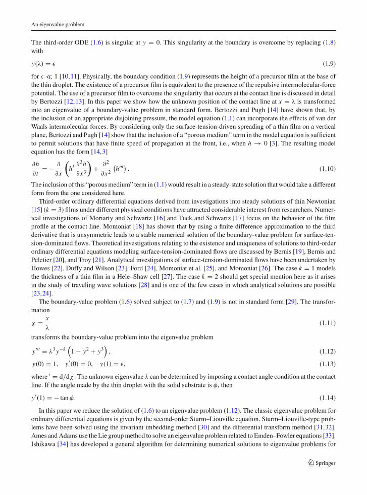
which models the spreading of the free surface h(x, t) of a thin film where x is the spatial coordinate and t is time.The partial differential equation (1.1) models the spreading of a thin film on a vertical slope [1]. The effects ofsurface shear, gravity, and surface tension have been included. The surface shear can be caused by an external forcesuch as wind, or it may arise due to temperature or concentration gradients [2]. The flux f (h) is given by

f (h) = αh2 − βh3, (1.2)

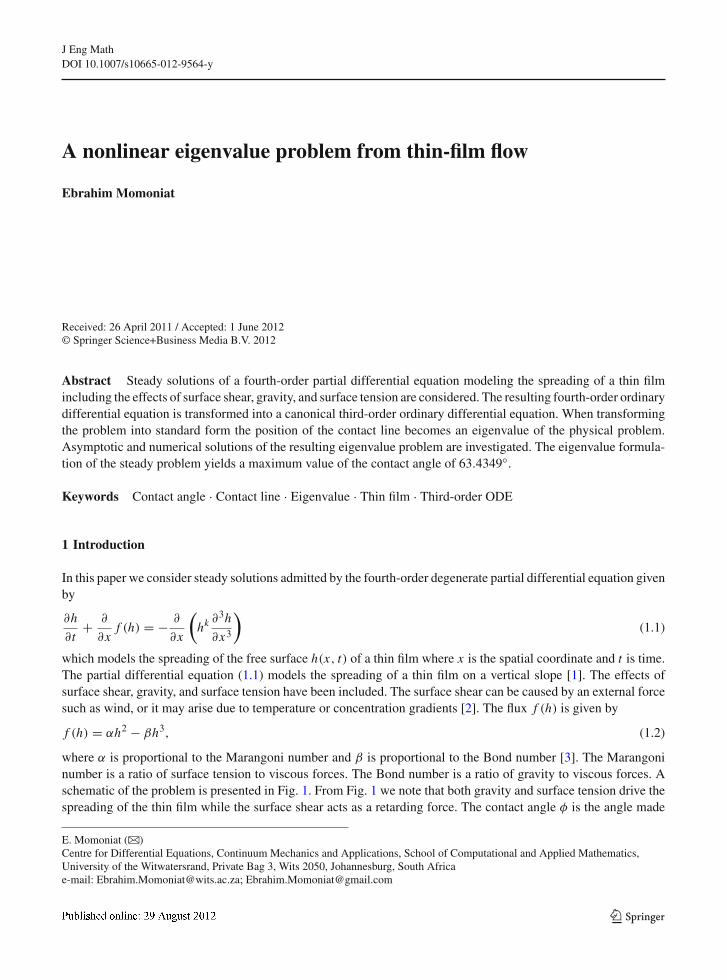
where α is proportional to the Marangoni number and β is proportional to the Bond number [3]. The Marangoninumber is a ratio of surface tension to viscous forces. The Bond number is a ratio of gravity to viscous forces. Aschematic of the problem is presented in Fig. 1. From Fig. 1 we note that both gravity and surface tension drive thespreading of the thin film while the surface shear acts as a retarding force. The contact angle φ is the angle made

E. Momoniat (B)Centre for Differential Equations, Continuum Mechanics and Applications, School of Computational and Applied Mathematics,University of the Witwatersrand, Private Bag 3, Wits 2050, Johannesburg, South Africae-mail: Ebrahim.Momoniat@wits.ac.za; Ebrahim.Momoniat@gmail.com

123

E. Momoniat

Fig. 1 Schematicof the problem

surface tension

surface shear gravity

x=0 x=r

φ

precursor film

free surface h(x,t)

between the thin film and the solid substrate on which the thin film is spreading. The significance of the precursorfilm is discussed later.

Reviews on physical applications of (1.1) can be found in Oron et al. [4] and Myers [3]. Derivations of (1.1)for surface-tension-dominated flows, surface shear effects, and gravity-dominated flows can be found in Bertozzi[1] and Myers et al. [5,6]. Experimental results for moving fronts modeled by (1.1) are presented in Kataoka andTroian [7]. The references indicated above focus on thin Newtonian fluids where k = 3. King [8] has shown thatthe high-order nonlinear diffusion term in (1.1) models shear-thinning flows for k > 3 and shear-thickening flowsfor 2 < k < 3. Physical situations in which steady solutions occur are typified by coating flows [3]. Kataoka andTroian [7] have shown in their experimental work that steady profiles are obtained when viscous, capillary, andMarangoni stresses balance. An example of a thin film flowing down a vertical wall and reaching a steady state ispaint drying on a wall [3].

In this paper we are interested in modeling the behavior of steady solutions of (1.1). Substituting the steadysolution

h(x, t) = y(x) (1.3)

into (1.1) we obtain

d

dx

(yk d3 y

dx3 + αy2 − βy3)

= 0. (1.4)

Substituting the transformations

y = α

βy, x = α(k−2)/3β(1−k)/3 x (1.5)

into (1.4) and integrating we obtain

yk d3 y

dx3 + y2 − y3 = 1, (1.6)

where we suppress the bars on y and normalize the integrating constant to 1.In this paper we are interested in solving (1.6) for boundary conditions related to the steady profile of a thin

droplet. Unlike the experimental work done on moving fronts by Kataoka and Troian [7], Tanner [9] performedexperimental work on the spreading of thin oil droplets. Some of this experimental work is also reported in the bookby Middleman [10, Chap. 7]. The boundary conditions from Tanner [9] are given by

dy(0)

dx= 0, y(0) = 1. (1.7)

The boundary conditions (1.7) from Tanner [9] are for spreading on a horizontal plane where symmetric spreadingoccurs. In the context of a thin film on a vertical plane, the boundary conditions (1.7) separate the leading edgefrom the bulk of the film. We do not consider the trailing-edge contact angle in this presentation. The remainingboundary condition comes from the height of the film at the unknown position of the contact line x = λ. Thisboundary condition is given by

y(λ) = 0. (1.8)

123123

An eigenvalue problem

The third-order ODE (1.6) is singular at y = 0. This singularity at the boundary is overcome by replacing (1.8)with

y(λ) = ε (1.9)

for ε � 1 [10,11]. Physically, the boundary condition (1.9) represents the height of a precursor film at the base ofthe thin droplet. The existence of a precursor film is equivalent to the presence of the repulsive intermolecular-forcepotential. The use of a precursor film to overcome the singularity that occurs at the contact line is discussed in detailby Bertozzi [12,13]. In this paper we show how the unknown position of the contact line at x = λ is transformedinto an eigenvalue of a boundary-value problem in standard form. Bertozzi and Pugh [14] have shown that, bythe inclusion of an appropriate disjoining pressure, the model equation (1.1) can incorporate the effects of van derWaals intermolecular forces. By considering only the surface-tension-driven spreading of a thin film on a verticalplane, Bertozzi and Pugh [14] show that the inclusion of a “porous medium” term in the model equation is sufficientto permit solutions that have finite speed of propagation at the front, i.e., when h → 0 [3]. The resulting modelequation has the form [14,3]

∂h

∂t= − ∂

∂x

(hk ∂3h

∂x3

)+ ∂2

∂x2

(hm)

. (1.10)

The inclusion of this “porous medium” term in (1.1) would result in a steady-state solution that would take a differentform from the one considered here.

Third-order ordinary differential equations derived from investigations into steady solutions of thin Newtonian[15] (k = 3) films under different physical conditions have attracted considerable interest from researchers. Numer-ical investigations of Moriarty and Schwartz [16] and Tuck and Schwartz [17] focus on the behavior of the filmprofile at the contact line. Momoniat [18] has shown that by using a finite-difference approximation to the thirdderivative that is unsymmetric leads to a stable numerical solution of the boundary-value problem for surface-ten-sion-dominated flows. Theoretical investigations relating to the existence and uniqueness of solutions to third-orderordinary differential equations modeling surface-tension-dominated flows are discussed by Bernis [19], Bernis andPeletier [20], and Troy [21]. Analytical investigations of surface-tension-dominated flows have been undertaken byHowes [22], Duffy and Wilson [23], Ford [24], Momoniat et al. [25], and Momoniat [26]. The case k = 1 modelsthe thickness of a thin film in a Hele–Shaw cell [27]. The case k = 2 should get special mention here as it arisesin the study of traveling wave solutions [28] and is one of the few cases in which analytical solutions are possible[23,24].

The boundary-value problem (1.6) solved subject to (1.7) and (1.9) is not in standard form [29]. The transfor-mation

χ = x

λ(1.11)

transforms the boundary-value problem into the eigenvalue problem

y′′′ = λ3 y−k(

1 − y2 + y3)

, (1.12)

y(0) = 1, y′(0) = 0, y(1) = ε, (1.13)

where ′ = d/dχ . The unknown eigenvalue λ can be determined by imposing a contact angle condition at the contactline. If the angle made by the thin droplet with the solid substrate is φ, then

y′(1) = − tan φ. (1.14)

In this paper we reduce the solution of (1.6) to an eigenvalue problem (1.12). The classic eigenvalue problem forordinary differential equations is given by the second-order Sturm–Liouville equation. Sturm–Liouville-type prob-lems have been solved using the invariant imbedding method [30] and the differential transform method [31,32].Ames and Adams use the Lie group method to solve an eigenvalue problem related to Emden–Fowler equations [33].Ishikawa [34] has developed a general algorithm for determining numerical solutions to eigenvalue problems for

123

E. Momoniat

second-order ordinary differential equations. An illustration of an application of a shooting method to fourth-ordereigenvalue problems is presented in Jones [35].

The paper is structured as follows. In Sect. 2 we consider an asymptotic solution to the eigenvalue problem(1.12) solved subject to (1.13) and (1.14). In Sect. 3 we consider a numerical solution of the eigenvalue problem.Concluding remarks are made in Sect. 4.

2 Asymptotic solution

In this section we determine an asymptotic solution to (1.12) at the contact line. We substitute

y′ = v(y) (2.1)

into (1.12) to obtain the second-order ordinary differential equation

v2 d2v

dy2 + v

(dv

dy

)2

= λ3(

y−k − y2−k + y3−k)

. (2.2)

The substitution (2.1) transforms the boundary conditions (1.13) and (1.14) into

v(ε) = − tan φ, v(1) = 0. (2.3)

To investigate the asymptotic behavior of (2.2) at the contact line we make the coordinate transformation

y = eξ . (2.4)

The second-order ordinary differential equation (2.2) is transformed into

v2(

d2v

dξ2 − dv

dξ

)+ v

(dv

dξ

)2

= λ3(

e(2−k)ξ − e(4−k)ξ + e(5−k)ξ)

. (2.5)

The asymptotic solution at the contact line y = 0 is investigated by taking ξ → −∞. For k < 2 and takingξ → −∞ in (2.5) we obtain

v2(

d2v

dξ2 − dv

dξ

)+ v

(dv

dξ

)2

= 0. (2.6)

Equation (2.4) transforms the boundary conditions (2.3) into

v (ln ε) = − tan φ, v(0) = 0. (2.7)

Solving (2.6) and imposing (2.7) we obtain

v(ξ) = −√

1 − eξ

1 − εtan φ. (2.8)

We note here that the boundary condition relevant to the asymptotic solution at the contact line is the boundarycondition specified at ξ = ln ε. We use the boundary condition at ξ = 0 to determine the unknown constant ofintegration in the solution of the second-order ordinary differential equation (2.6). We show later by comparisonwith the numerical solution that the asymptotic behavior of the solution at the contact line obtained here is correcteven though we have included the boundary condition at ξ = 0 when calculating this asymptotic solution. Physicallythis is correct as the bulk of the fluid is situated at ξ = 0 and hence the steady film shape will remain unchanged atthis position. The film shape at the contact line will vary with changing value of k.

Using (2.4) and (2.1) we can map (2.8) back to the original variables to obtain the first-order ordinary differentialequation

y′ = −√

1 − y

1 − εtan φ. (2.9)

123123

An eigenvalue problem

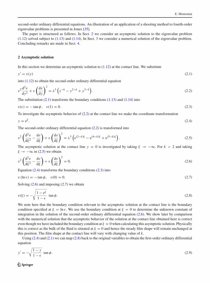
Fig. 2 Plot of the solution(2.10) for ε = 0.005 andvalues of the contact angleφ = [10, 20, 30, 40◦]

0.9 0.92 0.94 0.96 0.98 10

0.03

0.06

0.09ε=0.005

χ

y

φ=10°,20°,30°,40°

Solving the first-order ordinary differential equation (2.9) for y yields a quadratic equation. Physically meaningfulsolutions arise for the negative branch of the solution given by

y = ε − (χ − 1) tan φ + (χ − 1)2 tan2 φ

4 (ε − 1), (2.10)

where we have solved (2.9) subject to y(1) = ε. We note from (2.10) that in the vicinity of the contact line fork < 2 the solution is linear. We plot the solution (2.10) in Fig. 2 for ε = 0.005 for different values of the contactangle.

We now consider the case k = 2. Taking ξ → −∞ in (2.5) we obtain

v2(

d2v

dξ2 − dv

dξ

)+ v

(dv

dξ

)2

= λ3. (2.11)

To make analytical progress we investigate approximate solutions to (2.11) of the form

v(ξ) = v0(ξ) + λ3v1(ξ) + . . . , λ3 � 1. (2.12)

Substituting (2.12) into (2.11) and separating by coefficients to first order in powers of λ3 we obtain the system

v20

(d2v0

dξ2 − dv0

dξ

)+ v0

(dv0

dξ

)2

= 0, (2.13)

v20

(d2v1

dξ2 − dv1

dξ

)+ 2v0v1

(d2v0

dξ2 − dv0

dξ

)+ 2v0

dv0

dξ

dv1

dξ+ v1

(dv0

dξ

)2

= 1. (2.14)

Substituting the boundary conditions (2.7) into (2.12) and separating to leading order by coefficients in powers ofλ3 we obtain

v0 (ln ε) = − tan φ, v0(0) = 0, (2.15)

and

v1 (ln ε) = 0, v1(0) = 0. (2.16)

Solving (2.13) subject to (2.15) we obtain

v0(ξ) = −√

1 − eξ

1 − εtan φ. (2.17)

Substituting (2.17) into (2.14) we obtain the second-order ordinary differential equation

4(eξ − 1

) ((eξ − 1

) d2v1

dξ2 tan2 φ + dv1

dξtan2 φ − ε + 1

)− e2ξ v1 tan2 φ = 0. (2.18)

123

E. Momoniat

Solving (2.18) subject to (2.16) we obtain

v1 = ω−2[√

1 − ω2 cot2 φ

(ω (ε − 1) cosh(ξ/2) log 2

−(1 + ω2)√

(1 − ω2)−1 − 1 (ε − 1) log(

2(√

1 − ω2 +√

(1 − ω2)−1 − 1))

−(

2ω√

1 − ε + 2(ε − 1) + ω log 2(1 + ε) +2ω (ε − 2) log(

2(√

ε−1 − 1 + ε−1)))

sinh(ξ/2)

)], (2.19)

where

ω =√

1 − eξ . (2.20)

These results have been verified using the Mathematica symbolic algebra program.We invert the transformation (2.4) by taking ξ = log y. Substituting ξ = log y into the asymptotic solution (2.12)

and (2.1) we obtain an approximation to the first integral for k = 2 given by

y′ ≈ v0 (log y) + λ3v1 (log y) . (2.21)

We can solve the first-order ordinary differential equation from (2.21) by integrating∫dy

v0 (log y) + λ3v1 (log y)=

∫dχ. (2.22)

Using the fact that λ3 � 1 we can approximate the integral in (2.22) by∫dy

v0 (log y)− λ3

∫v1 (log y)

v20 (log y)

dy = χ + γ, (2.23)

where γ is a constant of integration. Evaluating (2.23) we obtain

−2√

y − 1 cot φ√

ε − 1 + λ3 (1 − y)−1/2[

2 (ε − 1) cot4 φ

(− √

1 − ε(y − 1) − (y + ε − 2) log 2

− (ε − 2)(y − 1) log(

2(√

ε−1 − 1+√

ε−1))

+(ε − 1)y log

(2

(√y−1 − 1+

√y−1

)) )]= χ+γ. (2.24)

We determine γ by imposing the condition y = 1 at x = 0 to find that

γ = 2 (ε − 1)2 λ3 cot4 φ. (2.25)

Even though we have obtained an implicit solution given by (2.24), this solution is only valid at the contact line.From this solution we can obtain a maximum value of the value of the contact angle by setting λ → 0, y → ε, andx → 1 in (2.24) to find

− 2 (ε − 1) cot φ = 1. (2.26)

We therefore find that the maximum value of φ = φmax depends on ε, where

φmax = arccot

[1

2 (1 − ε)

]. (2.27)

By taking the limit ε → 0 in (2.27) we find that φmax = φ∗ = 63.4349◦.In this section we have shown that asymptotic solutions are possible only for k ≤ 2. For k ≤ 2 the thin droplet has

a quadratic profile at the contact line. This compares well to the asymptotic solutions obtained by Duffy and Wilson[23] who investigate steady analytical solutions to the generalized lubrication equation for k = 2 solved subject toTanner’s boundary conditions. We have also shown that the eigenvalue problem which scales the maximum valueof x to 1 yields a maximum contact angle of φ∗ = 63.4349◦. We explore this further for different values of k in thenext section.

123123

An eigenvalue problem

0 10 20 30 40 50 600

0.5

1

1.5

2

2.5

φ

λ

k=0

k=1

k=2

k=3

φ *

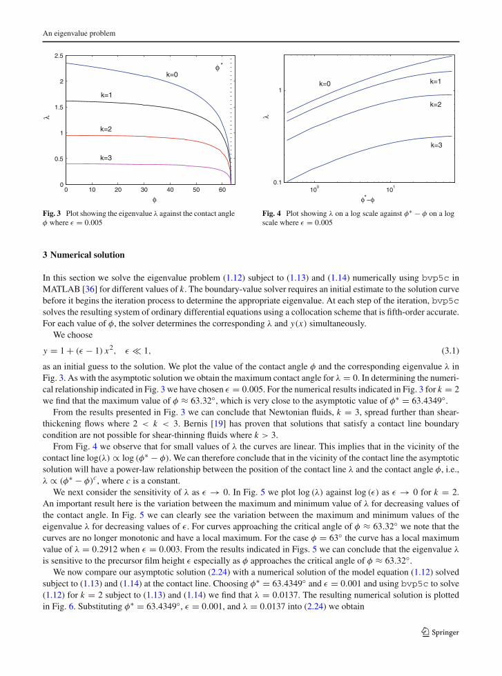
Fig. 3 Plot showing the eigenvalue λ against the contact angleφ where ε = 0.005

100

101

1

0.1

φ*−φ

λ

k=1k=0

k=3

k=2

Fig. 4 Plot showing λ on a log scale against φ∗ − φ on a logscale where ε = 0.005

3 Numerical solution

In this section we solve the eigenvalue problem (1.12) subject to (1.13) and (1.14) numerically using bvp5c inMATLAB [36] for different values of k. The boundary-value solver requires an initial estimate to the solution curvebefore it begins the iteration process to determine the appropriate eigenvalue. At each step of the iteration, bvp5csolves the resulting system of ordinary differential equations using a collocation scheme that is fifth-order accurate.For each value of φ, the solver determines the corresponding λ and y(x) simultaneously.

We choose

y = 1 + (ε − 1) x2, ε � 1, (3.1)

as an initial guess to the solution. We plot the value of the contact angle φ and the corresponding eigenvalue λ inFig. 3. As with the asymptotic solution we obtain the maximum contact angle for λ = 0. In determining the numeri-cal relationship indicated in Fig. 3 we have chosen ε = 0.005. For the numerical results indicated in Fig. 3 for k = 2we find that the maximum value of φ ≈ 63.32◦, which is very close to the asymptotic value of φ∗ = 63.4349◦.

From the results presented in Fig. 3 we can conclude that Newtonian fluids, k = 3, spread further than shear-thickening flows where 2 < k < 3. Bernis [19] has proven that solutions that satisfy a contact line boundarycondition are not possible for shear-thinning fluids where k > 3.

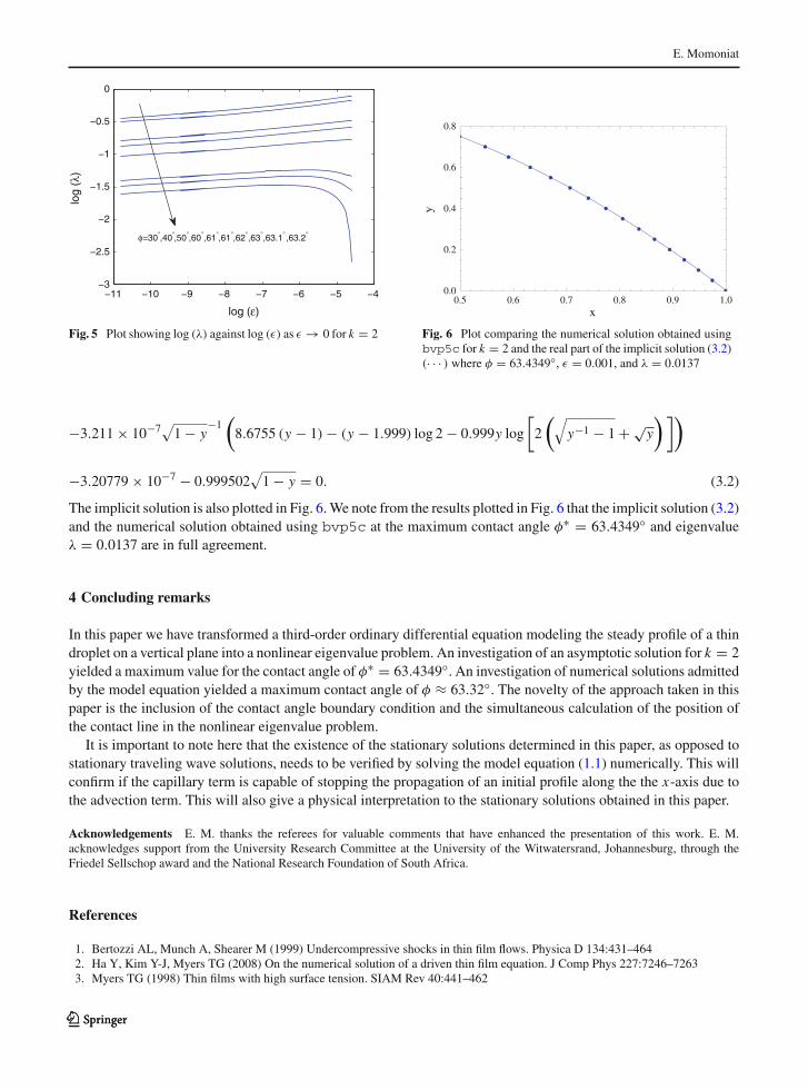
From Fig. 4 we observe that for small values of λ the curves are linear. This implies that in the vicinity of thecontact line log(λ) ∝ log (φ∗ − φ). We can therefore conclude that in the vicinity of the contact line the asymptoticsolution will have a power-law relationship between the position of the contact line λ and the contact angle φ, i.e.,λ ∝ (φ∗ − φ)c, where c is a constant.

We next consider the sensitivity of λ as ε → 0. In Fig. 5 we plot log (λ) against log (ε) as ε → 0 for k = 2.An important result here is the variation between the maximum and minimum value of λ for decreasing values ofthe contact angle. In Fig. 5 we can clearly see the variation between the maximum and minimum values of theeigenvalue λ for decreasing values of ε. For curves approaching the critical angle of φ ≈ 63.32◦ we note that thecurves are no longer monotonic and have a local maximum. For the case φ = 63◦ the curve has a local maximumvalue of λ = 0.2912 when ε = 0.003. From the results indicated in Figs. 5 we can conclude that the eigenvalue λ

is sensitive to the precursor film height ε especially as φ approaches the critical angle of φ ≈ 63.32◦.We now compare our asymptotic solution (2.24) with a numerical solution of the model equation (1.12) solved

subject to (1.13) and (1.14) at the contact line. Choosing φ∗ = 63.4349◦ and ε = 0.001 and using bvp5c to solve(1.12) for k = 2 subject to (1.13) and (1.14) we find that λ = 0.0137. The resulting numerical solution is plottedin Fig. 6. Substituting φ∗ = 63.4349◦, ε = 0.001, and λ = 0.0137 into (2.24) we obtain

123

E. Momoniat

−11 −10 −9 −8 −7 −6 −5 −4−3

−2.5

−2

−1.5

−1

−0.5

0

log (ε)

log

(λ)

φ=30°,40°,50°,60°,61°,61°,62°,63°,63.1°,63.2°

Fig. 5 Plot showing log (λ) against log (ε) as ε → 0 for k = 2

0.5 0.6 0.7 0.8 0.9 1.00.0

0.2

0.4

0.6

0.8

x

y

Fig. 6 Plot comparing the numerical solution obtained usingbvp5c for k = 2 and the real part of the implicit solution (3.2)(· · · ) where φ = 63.4349◦, ε = 0.001, and λ = 0.0137

−3.211 × 10−7√

1 − y−1

(8.6755 (y − 1) − (y − 1.999) log 2 − 0.999y log

[2

(√y−1 − 1 + √

y

)])

−3.20779 × 10−7 − 0.999502√

1 − y = 0. (3.2)

The implicit solution is also plotted in Fig. 6. We note from the results plotted in Fig. 6 that the implicit solution (3.2)and the numerical solution obtained using bvp5c at the maximum contact angle φ∗ = 63.4349◦ and eigenvalueλ = 0.0137 are in full agreement.

4 Concluding remarks

In this paper we have transformed a third-order ordinary differential equation modeling the steady profile of a thindroplet on a vertical plane into a nonlinear eigenvalue problem. An investigation of an asymptotic solution for k = 2yielded a maximum value for the contact angle of φ∗ = 63.4349◦. An investigation of numerical solutions admittedby the model equation yielded a maximum contact angle of φ ≈ 63.32◦. The novelty of the approach taken in thispaper is the inclusion of the contact angle boundary condition and the simultaneous calculation of the position ofthe contact line in the nonlinear eigenvalue problem.

It is important to note here that the existence of the stationary solutions determined in this paper, as opposed tostationary traveling wave solutions, needs to be verified by solving the model equation (1.1) numerically. This willconfirm if the capillary term is capable of stopping the propagation of an initial profile along the the x-axis due tothe advection term. This will also give a physical interpretation to the stationary solutions obtained in this paper.

Acknowledgements E. M. thanks the referees for valuable comments that have enhanced the presentation of this work. E. M.acknowledges support from the University Research Committee at the University of the Witwatersrand, Johannesburg, through theFriedel Sellschop award and the National Research Foundation of South Africa.

References

1. Bertozzi AL, Munch A, Shearer M (1999) Undercompressive shocks in thin film flows. Physica D 134:431–4642. Ha Y, Kim Y-J, Myers TG (2008) On the numerical solution of a driven thin film equation. J Comp Phys 227:7246–72633. Myers TG (1998) Thin films with high surface tension. SIAM Rev 40:441–462

123123

An eigenvalue problem

4. Oron A, Davis SH, Bankoff SG (1997) Long-scale evolution of thin liquid films. Rev Modern Phys 69:931–9805. Myers TG, Charpin JPF, Thompson CP (2002) Slowly accreting ice due to supercooled water impacting on a cold surface. Phys

Fluids 14:240–2566. Myers TG, Charpin JPF, Chapman SJ (2002) The flow and solidification of a thin fluid film on an arbitrary three-dimensional

surface. Phys Fluids 14:2788–28037. Kataoka DE, Troian SM (1997) A theoretical study of instabilities at the advancing front of thermally driven coating films. J Colloid

Interf Sci 192:350–3628. King JR (2001) Two generalisations of the thin film equation. Math Comput Model 34:737–7569. Tanner LH (1979) The spreading of silicone oil drops on horizontal surfaces. J Phys D 12:1473–1484

10. Middleman S (1995) Modeling axisymmetric flows: dynamics of films, jets, and drops. Academic, New York11. Myers TG, Charpin JPF (2000) The effect of the Coriolis force on axisymmetric rotating thin film flows. Int J Non-linear Mech

36:629–63512. Bertozzi AL (1996) Symmetric singularity formation in lubrication-type equations for interface motion. SIAM J Appl Math 56:681–

71413. Bertozzi AL (1998) The mathematics of moving contact lines in thin liquid films. Not Am Math Soc 45:689–69714. Bertozzi AL, Pugh M (1994) The lubrication approximation for thin viscous films: the moving contact line with a “porous media”

cut off of van der Waals interactions. Nonlinearity 7:1535–156415. Greenspan HP (1978) On the motion of a small viscous droplet that wets a surface. J Fluid Mech 84:125–14316. Moriarty JA, Schwartz LW (1992) Effective slip in numerical calculations of moving-contact-line problems. J Eng Math 26:81–8617. Tuck EO, Schwartz LW (1990) Numerical and asymptotic study of some third-order ordinary differential equations relevant to

draining and coating flows. SIAM Rev 32:453–46918. Momoniat E (2011) Numerical investigation of a third-order ODE from thin film flow. Meccanica 46:313–32319. Bernis F (1996) Finite speed of propagation for thin viscous flow when 2 < n < 3. C R Acad Sci I 322:1169–117420. Bernis F, Peletier LA (1996) Two problems from draining flows involving third-order ordinary differential equations. SIAM J Math

Anal 27:515–52721. Troy WC (1993) Solutions of third-order differential equations relevant to draining and coating flows. SIAM J Math Anal 24:155–

17122. Howes FA (1983) The asymptotic solution of a class of third-order boundary value problems arising in the theory of thin film flows.

SIAM J Appl Math 43:993–100423. Duffy BR, Wilson SK (1997) A third-order differential equation arising in thin-film flows and relevant to Tanner’s Law. Appl Math

Lett 10:63–6824. Ford WF (1992) A third-order differential equation. SIAM Rev 34:121–12225. Momoniat E, Selway TA, Jina K (2007) Analysis of adomian decomposition applied to a third-order ordinary differential equation

from thin film flow. Nonlin Anal A 66:2315–232426. Momoniat E (2009) Symmetries, first integrals and phase planes of a third order ordinary differential equation from thin film flow.

Math Comput Model 49:215–22527. Constantin P, Dupont TF, Goldstein RE, Kadanoff LP, Shelley MJ, Zhou SM (1993) Droplet breakup in a model of the Hele-Shaw

cell. Phys Rev E 47:4169–418128. Buckingham R, Shearer M, Bertozzi A (2003) Thin film traveling waves and the Navier slip condition. SIAM J Appl Math 63:722–

74429. Ascher U, Russell RD (1981) Reformulation of boundary value problems into “standard” form. SIAM Rev 23:238–25430. Scott MR (1973) An initial value method for the eigenvalue problem for systems of ordinary differential equations. J Comput Phys

12:334–34731. Abdel-Halim Hassan IH (2002) On solving some eigenvalue problems by using a differential transformation. Appl Math Comput

127:1–2232. Chen C-K, Ho S-H (1996) Application of differential transformation to eigenvalue problems. Appl Math Comput 79:173–18833. Ames WF, Adams E (1979) Non-linear boundary and eigenvalue problems for the Emden–Fowler equations by group methods.

Int J Nonlinear Mech 14:35–4234. Ishikawa H (2007) Numerical methods for the eigenvalue determination of second-order ordinary differential equations. J Comput

Appl Math 208:404–42435. Jones DJ (1993) Use of a shooting method to compute eigenvalues of fourth-order two-point boundary value problems. J Comput

Appl Math 47:395–40036. Shampine LF, Reichelt MW, Kierzenka J, Solving boundary value problems for ordinary differential equations in MATLAB with

bvp4c. www.mathworks.com/bvp_tutorial. Accessed 25 April 2011

123