CHAPTER 3

A non-steady state model of early

diagenesis including compaction and biological mixing

Introduction Within the geosciences, it has long been recognized that biological activity can modify the texture, structure and composition of surface sediments. Darwin (1881) already examined the stirring of soils by the burrowing of earthworms and made detailed observations on the way these organisms affect geological processes (see e.g. Guinasso and Schink, 1975 for an historical evocation of early studies on the effect of organisms on soils and sediments). Similar to terrestrial soils, the water-saturated sediments of marine, lacustrine and riverine environments show a comparable abundance of organisms, which are capable of mixing and transforming sedimentary material in diverse ways. In recent decades, there is a growing demand for a proper quantification of geochemical processes in surface sediments, as can be judged from the proliferation of so-called general early diagenetic models (e.g. Soetaert et al, 1996a; Van Cappellen and Wang, 1996; Boudreau, 1996a; Wijsman et al., 2001). The term early diagenesis refers to the combination of physical, chemical and biological processes that occur in the topmost layer of surface sediments following deposition (Berner, 1980). As biological activity plays a central role in surface sediment geochemistry, a prime concern in these modelling efforts constitutes an adequate incorporation of the influence of benthic organisms on the sediment. One important effect constitutes the biological reworking of sediments, a process that is commonly termed bioturbation (Richter, 1952; Aller, 1977). Bioturbation results from a wide range of animal behaviour and includes many different kinds of displacements, both in the fluid and the solid phase. Bioturbational activities comprise burrow and tube excavation (including the ultimate collapse and refilling of these tubes), crawling and ploughing through the sediment, swimming and moving of the interstitial fauna, the building of mounds and the digging of craters. Conventionally bioturbation is classified as “local” or “non-local”, based on the average distance the sediment is displaced by the organisms (Boudreau, 1986a). In chapter [2] however we have proposed a more consistent classification of biological activity into biological exchange and biological mixing, based on both ecological and thermodynamical grounds. Biological exchange was defined as the mass transfer between the organism and the surrounding sediment (i.e. both fluid and solid phase) i.e. the exchange of substances across the body lining of the organism. From an ecological viewpoint biological exchange is equivalent to the uptake and release of all kinds of metabolic substances (ingestion of food particles, defecation, uptake of O2, release of CO2…). Biological mixing then was introduced as the displacement of both fluids and

Chapter 3

66

solids due to contact with the body lining of the organisms. From an ecological viewpoint the process represents the sediment reworking induced by the appendages and other body parts, while the organism is moving in the sediment. In the mechanistic view of thermodynamics, the effective displacement of porewater and solid packages is actually the result of forces exerted by the organism on the surrounding sediment. Consequently, the term biological mixing can be regarded as a strict and mechanistic definition of bioturbation, which excludes certain types of sediment displacement often included in bioturbation (e.g. the ingestion/excretion of bulk sediment by deposit feeders). In this chapter we will solely focus on those activities that can be classified as biological mixing. In fact, early diagenetic modelling theory has a strong record of modelling biological mixing (Goldberg and Koide, 1962; Guinasso and Schink, 1975; Schink and Guinasso, 1977; Boudreau, 1986 a; see Boudreau, 1997 and 2000 for reviews). The commonly used description of biological mixing is based on a (molecular) diffusion analogy using Fick’s first law as a constitutive expression. Goldberg and Koide (1962) introduced this diffusive type of formulation as they envisioned the effect of biological mixing as a down-gradient transport of sediment tracer similar to molecular or turbulent eddy diffusion. Such diffusive theories have been particularly successful in quantifying the influence of the biota on the profiles of microtektite and radioactive tracers (e.g. Guinasso and Schink, 1975) and other solid phase constituents (e.g. Soetaert et al, 1996a; Van Cappellen and Wang, 1996; Boudreau, 1996a). Although the present theory on biological mixing modelling is already extensively developed, it can be regarded as both incomplete and inconsistent at some specific points. The present biological mixing theory is incomplete with respect to its influence on compaction, which constitutes an important physical transport process in sediments. Consolidation refers to the time-dependent deformation of the sediment skeleton as a result of its own weight. In fine-grained sediments compaction can create steep porosity gradients in the upper centimetres of the sediment (e.g. Mulsow et al., 1998). Such porosity gradients have significant effects on the early diagenesis of sediments (Jorgensen, 1978; Murray et al., 1978; Rabouille and Gaillard, 1991). However, present diagenetic theory is completely mass-based and fundamentally built on the ad-hoc approach of steady-state compaction. To avoid the formulation of a momentum balance for the sediment, the porosity profile is assumed constant in time, fitted to an empirical relation and treated as input to the early diagenetic model (this topic is discussed further and in more detail below). The special character of such an approach was clearly exposed in a paper by Boudreau and Bennett (1999), who stated that ‘scientists and engineers, who are interested in compaction and its effects on early diagenesis, need to confront the momentum-based compaction theory if we wish to have a non-ad hoc approach to porosity changes’. Moreover, early diagenetic modelling theory provides an inconsistent description of the relation between compaction and biological mixing. At present it is still an open question if and to what extent benthic organisms alter and influence porosity profiles. Boudreau (1986a) suggested two end-member relationships between porosity modification and biological mixing. The first possibility is that the biological mixing does not influence the porosity distribution and only acts to decrease concentrations gradients. This type of diffusive mixing is called intraphase mixing, as it mixes both the pore water and the solid phase separately. Porosity gradients then result from accumulation and compaction alone, independent of biological mixing. The second end-member type of biological mixing

A non-steady state model of early diagenesis

67

however does affect porosity profiles and is termed interphase mixing, because it acts to decrease porosity gradients by diffusively mixing the volume fraction of the fluid phase against the volume fraction of the solid phase. In the past, heated debates have taken place on how to combine compaction and biological mixing into an early diagenetic model (Christensen, 1983; Officer and Lynch, 1983; Carpenter, 1983) and the issue has continuously attracted interest in the past few decades (Boudreau, 1986a; Fukimori et al., 1992; Mulsow et al, 1998). Both mixing formulations have attracted supporters, but no conclusive answer has so far been provided as to their connection and consistent embedding into early diagenetic modelling theory. This paper aims at the development of a complete time-dependent theory of early diagenesis, which can fully account for both compaction and biological mixing. Given the fact that biological mixing is in effect a momentum transfer phenomenon which induces mixing and mass transfer, such a theory will be necessarily based on both mass and momentum considerations. To arrive at a consistent description of the simultaneous effect of both compaction and biological mixing, we have adopted a two-step approach. First we will derive a complete and non-steady state description of early diagenesis, based on the mass and momentum conservations presented in chapter [2]. Basically this approach requires the merging of classical diagenetic modelling theory (Berner, 1980; Boudreau, 1997) with the non-steady state theory of self-weight consolidation as known from geotechnical engineering (Biot, 1941; Gibson et al., 1967; Sharp, 1976; Gibson et al., 1981; Toorman, 1996). Subsequently, we will investigate how these equations need to be modified to arrive at the different formulations of biological mixing (either intraphase or interphase mixing) using an extension of the stochastic approach to biological mixing as pioneered by Boudreau (1986a).

The continuum approach The continuum description of surface and subsurface sediments is based on the general conservation equations for a multi-component, multi-phase system applied to a so-called porous medium (Bear, 1972; Bear and Bachmat, 1991; Gray and Hassanizadeh, 1998). Continuum theories of porous media generally distinguish between different scales of description (Cushman, 1997), classically the microscale (the scale at which each phase separately can be regarded a continuum i.e. µm-to-mm scale of sediment grains and the interstitial pores) and the macroscale (the scale at which the whole porous medium can be regarded a continuum i.e. the cm-to-m scale of the sediment, in hydrology also called Darcy-scale). At the grain scale the sediment is a highly heterogeneous medium, with clear physical discontinuities between sediment particles and the surrounding pore water. A rigid description on the microscale of the pore would, if not impossible, give little insight in the behaviour of the system as a whole. To conceive a manageable description of such a multi-phase medium, sediments are sampled and modelled at the macroscale (Bear, 1972; Bear and Bachmat, 1991; Lichtner, 1996). In fact, the continuum hypothesis is adopted on two consecutive levels: to transcend from the molecular level to the microscale continuum, and to go from the heterogeneous microscale to the macroscale. At the microscale, the collection of discrete molecules is replaced by a series of overlapping continua, one for each different species (multi-species continuum). At the macroscale the sediment is modelled by overlapping continua, each representing a different phase in the porous medium (multi-phase continuum). In this fictitious representation of the real physical

Chapter 3

68

system all the phases, and the different species within each phase, coexist at each point in space. Each of the continua fills the entire medium and to every point in space we may assign properties of any of the different continua (see general texts on multi-component, multi-phase continuum physics for more details on scaling e.g. Bear and Bachmat, 1991; Cushman, 1997). At the macroscale, reactive transport phenomena can be described by differential calculus and conservation equations stated as partial differential equations. This implies that the variables present in the macroscale model equations actually comprise averages of so called microscale quantities over a Representative Elementary Volume (REV). For example the concentration for the i-th chemical species in the α-th phase

( )1i i i

U

C C C r, t dUU α

ααα= = ∫ [3.1]

where Uα represents the subvolume within the REV occupied by the α-phase and

( )iC r, t refers to the microscale concentration. In an analogue way the volume fraction is defined as

1REV REV

U

UdU

U Uα

ααφ = =∫ [3.2]

where the total volume of the REV is defined as REVU Uα

α

= ∑ [3.3]

The volume fractions cannot be chosen independently, as they are related through the constraint of volume conservation

1α

α

φ =∑ [3.4]

The aim of continuum physics is to present a consistent set of conservation equations for the mass, momentum, energy and entropy in the system and to provide the appropriate constitutive expressions necessary to “close” the model statement. Over the past decades, two broad categories of continuum theories have been developed: the first approach postulates conservation equations directly at the macroscale, so-called mixture theory (Truesdell and Toupin, 1960; Bowen, 1977), while the second approach, the so-called volume averaging approach, starts at the microscale and arrives at the proper macro-scale conservation equation by an averaging procedure (Whitaker, 1967; Hassanizadeh and Gray, 1979a; Bear and Bachmat, 1986; Gray and Hassanizadeh, 1998).

A non-steady state model of early diagenesis

69

Multi-phase description of the sediment In chapter [2] we have extended the conventional two-phase (fluid/solid) description of surface sediments to multi-phase system approach, which included the benthic organisms as an additional phase 1. The explicit inclusion of the organisms in the model formulation was necessary to consistently describe the mass and momentum transfer between the benthos the surrounding sediment. Following the approach of chapter [2], we will adopt a three-phase description of the sediment, where f denotes the fluid phase, s denotes the solid phase and o denotes the organism phase. The volume balance for this system can be written as

1f s oφ + φ + φ = [3.5] The organisms however generally make up only a small fraction of the volume. Starting from 103 individual polychaet worms per m2 (in an estuarine system, Heip et al., 1995), assuming 2 mm diameter and a length of 3 cm, one obtains that the organisms make up for 2 % of the total volume. This justifies the exclusion of the organisms from the volume balance, but not from the other conservation equations.

1f sφ + φ ≈ [3.6] In chapter [2] the volume-averaging approach of continuum theory (Whitaker, 1967; Hassanizadeh and Gray, 1979a; Bear and Bachmat, 1986; Gray and Hassanizadeh, 1998) was used to arrive at a set of consistent macroscale mass and momentum conservations equations for the fluid phase and the solid phase in the presence of a separate organism phase. Here we will employ these conservations equations to construct a closed and functional mathematical model formulation for the surface sediments subject to compaction and biological mixing. The equations in this text will only incorporate macroscale quantities and therefore we can release the notational burden by dropping volume-averaging operator ...

α in the model formulation. Only when defining reference frames the volume-averaging operator will be occasionally used.

An instantaneous model of early diagenesis In chapter [2], the necessary conservation equations and constitutive expressions were derived for the fluid and the solid component of the three phase system fluids/solids/organisms. Our goal in this chapter is to integrate these equations into a practical model formulation of non-steady-state early diagenesis in accumulating sediments experiencing self-weight consolidation and biological mixing. In a first step however, we must investigate whether the equation set, formed by the approximated volume balance [3.6] and the mass and momentum conservation equations for the fluid and solid phase alone (i.e. not considering the conservation equation for the organism phase), effectively provides a closed mathematical model statement.

1 In this chapter, we are primarily concerned with mass and momentum interactions between the organisms on the one hand and the porewater and solid sediment phases on the other hand. Consequently we will not consider the gas phase as an additional phase in the description.

Chapter 3

70

The conservation of mass of a component The central conservation equation in surface geochemistry constitutes the mass balance for the i-th chemical species in the α-th phase (Bear and Bachmat, 1991). Such a mass balance must be stated for each chemical species in the fluid and solid phase of the three phase system fluids/solids/organisms. Assuming the fluid phase consists of nf chemical species and the solid phase incorporates ns chemical species, the total number of species in the fluid/solid phase amounts to n = nf + ns. In the field of early diagenesis this equation is referred to as the ‘general diagenetic equation’ (Berner, 1980; chapter [2]).

i i iC Jt

α α α α∂ φ + ∇ ⋅ = Γ ∂ i 1..nα= f ,sα = [3.7]

where the species mass flux iJ

α is given by i i iJ C vα α α α= φ [3.8]

In these expressions αφ denotes the volume fraction, iC

α represents the concentration and ivα denotes the so-called component velocity i.e. the averaged velocity over all the

molecules of a certain chemical species within a given representative elementary volume. The term i

αΓ must be interpreted as a general source-sink term, generated due to chemical reactions or biological exchange processes (Boudreau, 1997; chapter [2]). As biological mixing processes are the main focus of this communication, we will assume (without any loss of generality) that biological exchange is absent. Then the term i

αΓ represents the total production rate of a chemical species due to either homogeneous or heterogeneous reactions. For each reaction present, an appropriate kinetic description must be provided. In its most general form, this reaction term can be written as a function of the complete set of volume fractions and mass densities (see e.g. Lasaga, 1997 for details on particular kinetic expressions)

( )i i j,Cα α β βΓ = Γ φ j 1..nβ= f ,sβ = [3.9]

Assessing both the number unknowns and the available equations, the equation set [3.7]-[3.9] constitutes a mathematically underdetermined system, as it includes fewer equations than variables. The model includes only [n + 1] equations, consisting of the component mass balances [3.7] and the approximated volume balance [3.6], while there are [2n + 2] unknowns to be solved for, i.e. n species concentrations iC

α , n component velocities ivα ,

and 2 volume fractions αφ . In general there are two approaches possible to resolve this indeterminacy: either expanding the number of conservation equations, or increasing the number of constitutive expressions. The first possibility can be achieved by stating a momentum balance for each component separately. Some authors have explored this approach, which ultimately results in an additional partial differential equation for each component velocity iv

α (e.g. Kirwan and Kump, 1985; Hassanizadeh, 1996). However, the far more commonly employed approach is to introduce additional constitutive expressions, which in effect reduces the number of variables in the model, instead of increasing the number of conservation equations.

A non-steady state model of early diagenesis

71

This second approach then introduces a diffusive flux dif,riJ , which is defined with respect

to some reference velocity rv

( )dif,r ri i iJ C v vα α α= φ − [3.10]

Implementing [3.10], it is possible to decompose the total mass flux iJ

α into an advective part and a diffusive part with respect to the so-called reference frame rv

r dif,ri i iJ C v Jα α α= φ + [3.11]

The number of variables in the model is effectively reduced, if we are able to provide a diffusive constitutive expression of the general form

( )dif,r dif,ri i jJ J ,β β= φ ρ j 1..nβ= f ,sβ = [3.12]

The crucial point in the definition of the diffusive flux [3.10] concerns the choice of the reference velocity rv . In most cases the mass averaged velocity of a phase is used as the reference frame to scale diffusive fluxes. If we introduce the molecular mass iM , we can derive the total mass density of a phase as

1

n

i ii

MCα

α α

=

ρ = ∑ [3.13]

then the mass-averaged velocity m,v α can be calculated as

1

1 nm,

i i ii

vv MC v

αα

α α αα α

=

ρ= =

ρρ∑ [3.14]

Taking advantage of [3.13] and [3.14], the mass-averaged reference frame is characterized by the important property

( ) 0dif,m, m, m,i i i i i i i i i i

i i i i

MJ MC v v MC v v MCα α α α α α α α α α = φ − = φ − = ∑ ∑ ∑ ∑ [3.15]

Actually, the mass-averaged velocity is just one the many possible reference frames. Another commonly employed reference velocity is u,v α , the volume-averaged velocity of a phase, which is defined as

1

nu,

i i ii

v v U C vα

α α α α α

=

= = ∑ [3.16]

In [3.16] iU

α denotes the specific volume of a chemical species.

Chapter 3

72

Unlike in the mass-averaged reference frame, the total diffusive flux does not vanish in the volume-averaged frame

( )dif,u, m, u,i i

i

MJ v vα α α α α= φ ρ −∑ [3.17]

In general, one must carefully distinguish between reference velocities, as the constitutive expression [3.12] will depend upon the particular reference frame that is used. However, in most early diagenetic situations the density of both the pore water and the solid phase can be taken constant. Only in some special occasions (e.g. at high dissolution rates of CaCO3) the phase density change is significant enough to be effectively accounted for. The assumption of constant phase density is an important simplification, since for an “incompressible” phase both the mass averaged and volume averaged velocity become equivalent

1 1m, u,

U U

vv vdU vdU v v

UU α α

ααα α

α α αα

ρ= = ρ = = =

ρ ρ ∫ ∫ [3.18]

and consequently, one can simply speak of the phase velocity m, u,v v vα α α= = [3.19]

As a consequence, the mass-averaged and the volume-averaged reference frames become indistinguishable. From this point on, we will continue to adopt a constant density for both the fluid and the solid phase. Introducing the phase velocity reference frame, the corresponding diffusive flux becomes

( )dif,i i iJ C v vα α α α α= φ − [3.20]

and upon implementation of [3.20], the general diagenetic equation [3.7] becomes

dif,i i i iC C v J

tα α α α α α α∂ φ + ∇ ⋅ φ + = Γ ∂

[3.21]

Expression [3.21] constitutes the classical formulation of the so-called general diagenetic equation (Berner, 1975; Berner, 1980; Boudreau, 1997). Until now we did not make any assumption on the particular nature of the transport processes accounted for by the diffusive flux [3.20]. The small advective velocities commonly encountered in surface sediments lead to small Peclet numbers H

iPe (Boudreau, 1997; chapter [2])

1sed

Hi md

i

d vPe

D

α

= [3.22]

In the expression for the dimensionless Peclet number sedd denotes the average particle diameter of the sediments grains and md

iD denotes the molecular diffusion coefficient.

A non-steady state model of early diagenesis

73

When small Peclet numbers characterize the sediment environment, molecular diffusion generally dominates mechanical dispersion and the macroscale diffusive flux can be attributed following constitutive expression (chapter [2]) dif,f md f f eff fi i i i iJ D C C= ∇ = ∇T D [3.23]

In expression [3.23] we have introduced the effective diffusion tensor eff md f

i iD=D T , where fT denotes the tortuosity tensor. The expression for the diffusive flux resembles the classical formulation of the Fick’s first law of diffusion. A major distinction is that the scalar diffusion coefficient md

iD (which is independent of spatial configuration within the REV) is now replaced by a second-rank tensor eff

iD , which reflects the influence of the geometry of the porous medium on the molecular diffusion phenomenon. Regarding the solid sediment, we will assume there is no diffusive flux within the solid phase.

0dif,siJ = [3.24]

Note that we did not include biological mixing as a transport process in the formulation of the diffusive flux dif,

iJα . As was clearly demonstrated in chapter [2], biological mixing

constitutes a momentum transfer phenomenon and must be modelled via momentum transfer formalism in the momentum conservation equations. Consequently, in the instantaneous model formulation of early diagenesis, biological mixing does not show in the mass conservation equations. In fact, this conjecture forms the cornerstone of our newly proposed treatment of biological mixing. As it forms the key concept in this communication, it will be discussed in more detail in the coming sections. The conservation of total mass of a phase Making a new balance of both equations and unknowns, then the volume balance [3.4] and the diagenetic equations [3.21] combine to a set of [n + 1] equations, incorporating a total of [n + 4] variables i.e. 2 volume fractions αφ , 2 phase velocities vα and n concentrations iCα . This means we need three more equations to arrive at a mathematically closed model

statement. Two equations can be readily found by applying the general conservation principle to the fluid and solid phase as a whole (Bear and Bachmat, 1991; chapter [2])

vt

α α α α α α∂ φ ρ + ∇ ⋅ φ ρ = Γ ∂ f ,sα = [3.25]

where αΓ denotes a source/sink term due to heterogeneous reactions at the solid/fluid interfaces (recall that biological exchange was assumed absent). Expression [3.25] can equally be found through a proper summation of the individual component mass balances. As a consequence, the total source/sink term can be written as

i ii

Mα αΓ = Γ∑ [3.26]

Chapter 3

74

If we recall the assumption of constant density, then the total mass balance reduces to

vt

αα α α

α

∂ Γ φ + ∇ ⋅ φ = ∂ ρ [3.27]

Because of the principle of mass conservation, the heterogeneous reaction terms in fluid and solid phase must be of opposite sign f sΓ = −Γ [3.28]

When the bulk mass transfer due to heterogeneous reactions is negligible, then the summation of [3.27] for both phases results in

0f f s sv v ∇ ⋅ φ + φ = [3.29] Equation [3.29] simply expresses that when the phase density is constant and there is no interphase mass transfer (either due to heterogeneous reactions or biological exchange), the volume-averaged velocity U

f f s sU v v= φ + φ [3.30] of the whole sediment must remain constant. The phase mass balance equations [3.27] provide two additional relations for the model of early diagenesis. However, the combined volume [3.6], species mass [3.21] and phase mass [3.27] conservation equations constitute still a mathematically under-determined system, and thus needs an additional “closure” relation. Again two options are open: finding an extra conservation equation or introducing an additional constitutive relation. The second option is the standard approach in diagenetic modelling and is enabled by the postulate of steady-state compaction (Berner, 1980; Boudreau, 1997). The closure problem is then resolved by the introduction of a constitutive expression for either the porosity fφ or the solid volume fraction sφ , which is assumed to be time-independent. Commonly it takes the form

( )0x, ,α α α α∞φ = φ φ φ [3.31]

where 0

αφ and α∞φ are the volume fractions at the sediment-water interface and infinite

depth and x denotes the depth into the sediment. With the assumption of steady-state volume fractions and no fluid/solid interphase mass-transfer, equation [3.27] reduces to

0vα α ∇ ⋅ φ = [3.32] Combining the volume fraction profile [3.31] and the volume balance [3.6], the respective mass average velocities can be calculated from [3.32] when proper boundary conditions have been stated. Different empirical expressions have been proposed for the volume fraction profile [3.31], from which the exponential expression is the most commonly used (e.g. Rabouille and Gaillard, 1991; Fukimori et al., 1992). Recently Boudreau and Bennett (1999) advanced an inverse exponential expression based on a steady-state momentum balance for the sediment. The procedure based on steady-state compaction is also the

A non-steady state model of early diagenesis

75

standard method in a suite of complex general-purpose diagenetic models, which have emerged recently (Soetaert et al., 1996a; Boudreau, 1996a; Van Cappellen and Wang, 1996; Wijsman et al., 2001). However, in the geotechnical literature on compaction theory, a different approach is taken to the indeterminacy of the diagenetic system. The common practice there is to incorporate an additional conservation equation for the momentum of the porous medium, and not to provide an additional constitutive expression (like expression [3.31] for the volume fraction). Stated in a very general fashion, a momentum balance for a particular phase can be written as a relation Gα between the pressure p , the volume fraction and the phase velocity.

( ) 0G ,v ,pα α αφ = [3.33] If the momentum balances of both the pore water and solid phase are combined, it should be possible to eliminate pressure from [3.33] and to obtain a combined relation G , which represents the momentum balance for the whole sediment. In its most general form, the function G will relate both the phase volume fractions and the phase velocities

( ) 0f s f sG , ,v ,vφ φ = [3.34] The challenge then is to derive the proper functionality of G for surface sediments undergoing the process of self-weight compaction. For sediments which are not subject to biological mixing, such an expression is provided by the saturated stress balance from consolidation theory and soil mechanics (Gibson et al., 1967; Sharp, 1976; Gibson et al., 1981; Toorman, 1996). In the next section we will derive the equivalent of the saturated stress balance for a sediment experiencing biological mixing. The sediment momentum balance In chapter [2] the proper momentum conservation equations were obtained for both the fluid and solid phase of a sediment, which is simultaneously subject to biological mixing and compaction. These equations were derived from the general momentum conservation equation for the fluid/solid/organisms system through a consecutive series of reasonable simplifications specifically adapted to the problem of early diagenesis. The resulting momentum balances for respectively the porewater and the solid sediment are (see chapter [2] for details on their derivation) f f f M

f,s o,fp g z Fφ ∇ = φ ρ ∇ + Φ + [3.35] s s s M

ij f,s o,sp g z F′ φ ∇ = φ ρ ∇ + ∇ ⋅ σ − Φ + [3.36] where p denotes the porewater pressure, g the gravitational constant, the term f,sΦ expresses the drag force between the sediment grains and the surrounding porewater, ij′ σ denotes the intergranular stress tensor and the z-coordinate is directed downward.

Of special interest are the two biological stress terms: Mo,fF denotes the force exerted by the

organisms on the porewater within the REV and Mo,sF denotes a similar force exerted by

Chapter 3

76

the organisms on the solid sediment. The presence of these “biological” terms distinguishes the momentum equations [3.35] and [3.36] from the corresponding equations for an “abiotic” sediment, i.e. not subject to biological mixing. As was outlined in detail in chapter [2], the origin of these biological stress terms is unequivocally identified as biological mixing. Benthic organisms plough and crawl in the sediments and as a result of these activities, sediment grains and porewater “packages” are displaced. The conventional view is to interpret this biological mixing process as a mass transfer phenomenon. Indeed, at first sight and from a descriptive point of view, biological mixing is a mixing phenomenon, which tends to destroy concentration and (possibly) porosity gradients in the sediment. However, looking at biological mixing instantaneously and from a mechanistic point of view, it really constitutes a momentum-transfer phenomenon. To support this view, a detailed inspection of the underlying physical process is needed. At the microscale the effective displacement of porewater and solid packages is caused by pressure and shear forces between the body lining of the organisms and the surrounding environment. Due to the forces invoked by the organisms, both pore water “packages” and sediment grains are displaced, which then results in the observed mixing. Biological mixing thus closely resembles the phenomenon of turbulence in fluids, where the momentum transfer between the whirls causes differential velocities in the fluid, and thus results in mass transfer due to moving fluid packages. The primary effect of biological mixing is therefore the generation of rapid fluctuations in the velocity of fluid and the solid phases. The accompanying mixing phenomenon can be regarded as a secondary effect, since it is merely a consequence of the induced velocity variations. The momentum equations [3.35] and [3.36], correspond to this instantaneous/mechanistic view on biological mixing in terms of forces at the interface between organisms and sediment. The biological stress terms M

o,fF and Mo,sF are macroscale

stress terms, which account for the interfacial stresses between the “organism phase” and the fluid and solid phase integrated over a suitable REV (chapter [2]). It is noteworthy to mention that the biological stress terms can only emerge in the momentum conservation equations by explicitly incorporating the organisms as a third phase in the description. To integrate the momentum balances [3.35] and [3.36], constitutive expressions must be given for the fluid/solid drag force and the intergranular stress. When there is relative motion between the sediment particles and the fluid, there is momentum exchange between both phases because of friction at the contact surfaces. This drag is presented in the momentum equations as a general shear force from the fluid phase onto the solid phase, and is usually expressed by (Bear and Bachmat, 1991; chapter [2])

{ } ( )2f f sf,s v v

kµΦ = − φ − [3.37]

Expression [3.37] can be interpreted as an extension of Darcy's law from hydrology. When the biological interaction term M

o,fF is neglected in [3.35] and upon substitution of [3.37], one can show the momentum balance for the porewater reduces to Darcy's expression, originally proposed in 1856 (Bear and Bachmat, 1991; chapter [2]). For an isotropic medium, the granular stress tensor can be written as ij I′ ′ σ = σ , where ′σ is a scalar and I denotes the unity tensor. Then the divergence of the intergranular stress tensor becomes

sij s

′∂σ′ ∇ ⋅ σ = ∇φ ∂φ [3.38]

A non-steady state model of early diagenesis

77

The conventional constitutive expression for the intergranular stress is termed the rheological equation of state (Boudreau and Bennett, 1999).

( )ss s

′ ′∂σ ∂σ= φ∂φ ∂φ

[3.39]

The rheological equation of state models the self-weight consolidation of the sediment matrix and expresses the intergranular stress as a function of the solid volume fraction. The literature on compaction advances many empirical relations, mostly for low-porosity subsurface sediments (e.g. Terzaghi, 1942; Been and Sills, 1981; McVay et al., 1986), but recently a specific expression has been proposed for fine-grained marine surface sediments (Boudreau and Bennett, 1999). Here the actual form of [3.39] is not important, and we will assume an appropriate rheological equation of state is available. Implementing the fluid/solid drag term [3.37] and the rheological equation of state [3.39], it is possible to combine the momentum balance for the porewater and the solid phase to obtain a single momentum balance for the sediment, which no longer incorporates the unknown porewater pressure p . For this purpose the excess pore pressure ep is commonly introduced (Bear and Bachmat, 1991; Toorman, 1996). During consolidation the collapsing soil skeleton forces pore water to move out of the squeezed pores. As a result the pore water moves relatively to the particles, which in its turn generates the drag force f,sΦ . Due to the narrow drainage paths formed by the connecting pores, there is considerable friction and resistance to flow. Consequently there is an increase of the fluid pore pressure due to the weight of the solid particles and thus the pore pressure p can become significantly higher than the hydrostatic pressure. The excess pore pressure ep is defined as the difference between the actual porewater pressure and the hydrostatic pressure e fp p g z= − ρ ∇ [3.40]

The excess pressure is generated by the compaction of the sediment. Note that due to the drag force, the porewater movement also slows down the consolidation. Thus the presence of an excess pressure forms an indication that the consolidation process is still continuing (Toorman, 1996). If we introduce the excess pressure in the momentum balances [3.35] and [3.36] for the pore water and the solid phase, we obtain f e M

f,s o,fp Fφ ∇ = Φ + [3.41]

( )s e s s f Mf,s o,sp g z F′φ ∇ = φ ρ − ρ ∇ + ∇ ⋅ σ − Φ + [3.42]

Employing the explicit expression for the drag term [3.37], then expression [3.41] can be rewritten as

( ) 1e f f s Mo,ffp v v F

kµ∇ = − φ − +

φ [3.43]

If we neglect the biological interaction terms, expression [3.41] reduces to the so-called Darcy-Gersevanov law, introduced by Gersevanov (1934) in soil mechanics. In a similar

Chapter 3

78

way we can rearrange the momentum balance for the solid phase. The summation of the momentum balances [3.41] and [3.42] results in

( ) ( )e f s e s s f M Mo,s o,fp p g z F F′∇ ≈ φ + φ ∇ = φ ρ − ρ ∇ + ∇ ⋅ σ + + [3.44]

The approximation step in [3.44] employs the approximated volume balance [3.6], which is a crucial assumption at this point. Upon substitution of the Darcy-Gersevanov law [3.43] into the previous expression, and introducing the biological stress term bioF (where again the volume balance [3.6] in the approximation step)

1 sbio M M M M M

o,s o,f o,f o,s o,ff fF F F F F Fφ= + − ≈ −

φ φ [3.45]

we obtain following equation

( ) ( )s s f f f s biog z v v Fkµ′−∇ ⋅ σ = φ ρ − ρ ∇ + φ − + [3.46]

This expression describes how the effective stress on each layer of particles results from the downward force due to the buoyant weight of the particles, decreased by an upward drag force due to the flow of the fluid, and either enforced or diminished by the net force bioF of the organisms on the sediment. Without the biological stress term bioF , the

previous equation is known as the saturated soil stress balance known from soil mechanics (Toorman, 1996). By analogy we will refer to expression [3.46] as the saturated sediment stress balance or briefly the sediment momentum balance. A closed instantaneous model of early diagenesis Given the biologically corrected saturated sediment stress balance, the ambition now is to derive a proper dynamic compaction equation, which can account for the effect of biological mixing. Employing the definition [3.30] of the volume-averaged velocity U for the bulk sediment and using the approximated volume balance [3.6], we can rearrange following term

( ) ( )f f s f f s s s s f s f s s sv v v v v v U v U vφ − = φ + φ − φ − φ = − φ + φ ≈ − [3.47] Substituting [3.47] in the extended sediment momentum balance [3.46], one obtains

( ) ( )s s f s biog z U v Fkµ′−∇ ⋅ σ = φ ρ − ρ ∇ + − + [3.48]

which can be rearranged to obtain an explicit expression for the phase velocity of the solid sediment

( ){ }s s s f biokv U g z F′= + ∇ ⋅ σ + φ ρ − ρ ∇ +

µ [3.49]

A non-steady state model of early diagenesis

79

Making once more use of definition [3.30] for the volume-averaged velocity the previous expression can be also cast in the alternative form

( ){ }s

f s s f biof

kv U g z F

φ ′= + ∇ ⋅ σ + φ ρ − ρ ∇ +µφ

[3.50]

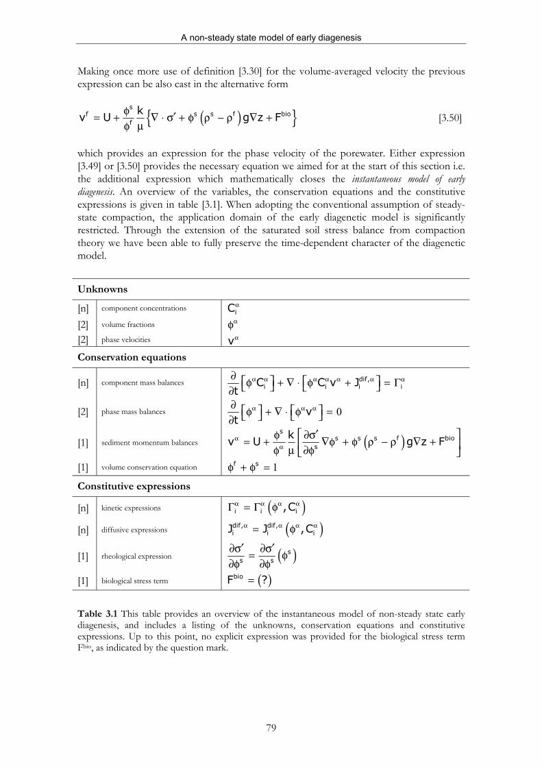
which provides an expression for the phase velocity of the porewater. Either expression [3.49] or [3.50] provides the necessary equation we aimed for at the start of this section i.e. the additional expression which mathematically closes the instantaneous model of early diagenesis. An overview of the variables, the conservation equations and the constitutive expressions is given in table [3.1]. When adopting the conventional assumption of steady-state compaction, the application domain of the early diagenetic model is significantly restricted. Through the extension of the saturated soil stress balance from compaction theory we have been able to fully preserve the time-dependent character of the diagenetic model.

Table 3.1 This table provides an overview of the instantaneous model of non-steady state early diagenesis, and includes a listing of the unknowns, conservation equations and constitutive expressions. Up to this point, no explicit expression was provided for the biological stress term Fbio, as indicated by the question mark.

Unknowns

[n] component concentrations iCα

[2] volume fractions αφ [2] phase velocities vα Conservation equations

[n] component mass balances dif,i i i iC C v J

tα α α α α α α∂ φ + ∇ ⋅ φ + = Γ ∂

[2] phase mass balances 0vt

α α α∂ φ + ∇ ⋅ φ = ∂

[1] sediment momentum balances ( )αα

′ φ ∂σ= + ∇φ + φ ρ − ρ ∇ + µφ ∂φ

ss s s f bio

s

kv U g z F

[1] volume conservation equation 1f sφ + φ = Constitutive expressions

[n] kinetic expressions ( )i i i,Cα α α αΓ = Γ φ

[n] diffusive expressions ( )dif, dif,i i iJ J ,Cα α α α= φ

[1] rheological expression ( )ss s

′ ′∂σ ∂σ= φ∂φ ∂φ

[1] biological stress term ( )bioF ?=

Chapter 3

80

Given the appropriate boundary conditions, the early diagenetic model as stated in table [3.1] permits a full description of early diagenesis, accounting for the ‘physical’ mass transfer processes of molecular diffusion and hydrodynamic dispersion, the ‘physical’ momentum transfer phenomena of fluid/solid drag and compaction and the ‘biological’ momentum transfer phenomenon of biological mixing. The presence of biological stress term bioF in the sediment momentum balance causes the phase velocity vα to deviate from the velocity the same phase would have, when no biological activity is present. Because biological mixing is regarded as a momentum transfer phenomenon, it enters the set of conservation equations through the sediment momentum balance, rather than via the mass balances. Consequently, biological mixing will not modify the instantaneous phase and species mass balances, although this may seem surprising at first sight (chapter [2]). The biological shear stresses will only influence the phase velocity fields and thus the influence of biological mixing will only penetrate the mass balances in an indirect way via these modified phase velocities. To enable the application of the sediment momentum balance an additional constitutive expression for the biological stress term is required (as denoted by the question mark in table [3.1]). The derivation of an explicit expression for bioF in terms of macroscale quantities however promises a complex and daunting task. Recall that bioF accounts for the momentum transfer across the surface lining of the organisms integrated within an REV. Organisms display a wide variety of shapes and geometries, and they also show a wide range of different activities and behaviour. As a consequence, an explicit characterization of bioF becomes virtually impossible. However, two properties of the biological stress term can be easily deduced: (1) it will constitute an intensely fluctuating property and (2) when averaged over time it must vanish, otherwise it would accelerate the sediment as a whole in a particular direction (which is not physically acceptable). Although no explicit expression can be deduced, these latter two properties make that the biological stress term can be modelled as a randomly fluctuating property. This implies that the current diagenetic model can be viewed as an instantaneous model driven by the rapidly fluctuating forcing function bioF . Instantaneous models are not convenient however, as they only provide a mathematical snapshot of sediment processes. Only the time-averaged behaviour of the system is of any practical interest. Similar to the phenomenon of turbulence, a stochastic approach is needed to obtain time-averaged model equations

Stochastic treatment of diagenesis Previously, we have mentioned the resemblance of biological mixing and turbulence, and indeed, we are faced with similar conceptual problems when applying the model from table [3.1] as when modelling fluid turbulence. Although the above model is valid at any instance, it is impossible to simulate the instantaneous path of a particular fluid or solid package, as it haphazardly soars away upon contact with a bioturbating animal. A description at all points in time and space is not feasible, and instead we will develop equations governing mean quantities, as was proposed by Reynolds (1894) to model turbulence. In the context of biological mixing, such an approach was pioneered by Boudreau (1986a), and later expanded upon by Boudreau (1997). Until present these treatments only consider the species mass conservation equations [3.21] in a stochastic fashion. Here we will adopt a broader perspective and additionally include the phase mass [3.27] and the newly derived sediment momentum conservation equation [3.50]. Stated

A non-steady state model of early diagenesis

81

otherwise, the instantaneous model of sediment diagenesis (see table [3.1]) will be used as the starting point for a stochastic analysis. Before we can apply the Reynolds method to biological mixing in porous media, we need to adopt a number of crucial assumptions:

1. There exists a “natural” scale of observation, where an appropriate model is available, which states both conservation equations and constitutive expressions. Here this scale coincides with the macroscale or Darcy-scale and we advance the instantaneous model summarized in table [3.1], as the appropriate instantaneous model at the macroscale.

2. Biological mixing will induce fluctuations in the microscale phase velocity due to microscale stresses, acting between the organisms and their surroundings. These microscale stresses are integrated to the macroscale by means of the biological stress term bioF . We assume that this biological stress term is a random fluctuating variable.

3. As a consequence of the sediment momentum equation [3.48], the randomness in the biological stress will be transmitted to the phase velocity, which then too becomes a random fluctuating variable.

4. Here we will impose an additional constraint on the phase velocity and assume that the macroscale phase velocity is a stationary random variable (though this constraint will be released in chapter [4]) Stationarity is defined as a quality of a process in which the statistical parameters of the process do not change with time. The most important property of a stationary variable is that the auto-correlation function depends on lag alone (see also appendix A).

Given the above assumptions, we are equipped to model the effect of biological mixing as a macroscale stochastic phenomenon i.e. the activity of the benthic organisms causes both the porewater and the solid sediment to fluctuate randomly around their (macroscale) phase velocity. The velocity fluctuations induced by biological mixing resemble the random fluctuations of turbulence and therefore biological mixing must be treated with similar statistical methods (e.g. Tennekes and Lumley, 1972). The instantaneous model derived in the previous section will be the starting point of our stochastic analysis. Subsequently we will investigate how the instantaneous model equations are affected when they are statistically averaged. There are two general approaches in developing statistical treatments of stochastic phenomena. The first gives expected values as time averages, while the second relies on an ensemble perspective in which a probability density function is defined and averages are taken with respect to this probability distribution (Cushman, 1997). Under the condition of ergodicity both approaches are equivalent. A stationary random function f is said to be ergodic if any statistical characteristic of the function, taken over a sufficiently large domain in a single realization, provides an unbiased and consistent estimate of the same characteristic over the entire set of possible realizations (Yaglom, 1965). If we denote the expectation operator by an overbar, then time averages equal expected values under the ergodic hypothesis

0

0

12

t T

t T

f f dtT

+

−

= ∫ [3.51]

Chapter 3

82

For the time-average to make sense, the averaging period T must be suitably chosen i.e. far larger than the time-scale of the fluctuations. Introducing the so-called Reynolds decomposition, the instantaneous value of physical variable can be written as the sum of a mean value and a fluctuation

ˆf f f= + [3.52] The mean value of a fluctuating quantity itself is zero

0

0

1 02

t T

t T

f̂ f f dt f fT

+

−

= − = − = ∫ [3.53]

One can also easily show that the mean value of a spatial or a temporal derivative is equal to the corresponding derivative of the mean value of that variable (Tennekes and Lumley, 1972). f ft t∂ ∂=∂ ∂

[3.54]

f f∇ = ∇ [3.55] These operations can be performed because averaging is carried out by integrating over a long period of time, which commutes with differentiation with respect to another variable.

Time-averaged biological mixing models The equations summarized in table [3.1] form a closed mathematical statement of early diagenesis in a bioturbated system and in principle they can be integrated and solved. However, in any practical situation this is not feasible. One difficulty arises instantly, since an appropriate constitutive expression for the biological stress term bioF must be provided. A second, more severe problem concerns the small time-scale, which the instantaneous model uses to provide a description of early diagenesis. Even if an appropriate constitutive expression for the biological stress term would be available and even if it would be possible (in terms of computer resources) to integrate the system of equations, the obtained output would be as impractical as the calculations difficult. In reality we are not interested in the instantaneous (rapidly fluctuating) values of the variables, but need time-averaged values for practical research purposes. Therefore we will restate the model in terms of “mean” variables in the sense of [3.51]. Mean conservation equations The central hypothesis underlying biological mixing is that the movement and activity of the benthic organisms will essentially generate shear stresses in the sediment environment. If one imagines that movements are randomly directed, a reasonable assumption could be that the time-average of the biological stress term vanishes.

A non-steady state model of early diagenesis

83

Then we can introduce the stress term as a true fluctuating property with zero mean bio bioF F= and 0bioF = [3.56]

In fact, expression [3.56] can be interpreted as a specific constitutive relation for the biological stress term. The uncertainty in the biological stress term will in turn generate random fluctuations in the phase velocity field via the sediment stress balance [3.48]. As was mentioned earlier, the phase velocity is introduced as a stationary random variable. Applying the Reynolds decomposition [3.52], it can be written as v v vα α α= + [3.57] We can expect these random fluctuations in the phase velocity to affect other phase properties, such as the volume fraction and the concentration fields within a phase. Stated in statistical terms, the uncertainty in the velocity field of a certain phase will result in uncertainty and randomness in the species concentrations and the volume fractions. Consequently we can also introduce the volume fractions and the species concentrations as stationary random variables

αα αφ = φ + φ [3.58]

i i iC C Cα α α= + [3.59] To result in practical model equations, we must (1) substitute the Reynolds expressions for the phase velocities [3.57], the volume fractions [3.58] and the species concentrations [3.59] in the instantaneous conservation equations, and (2) derive mean conservation equations by application of the time-averaging operator to the instantaneous equations. Starting with the volume conservation equation [3.6], the substitution of the Reynolds decomposition of the volume fractions results in

1f s f sφ + φ + φ + φ = [3.60]

If we apply the averaging operator to this instantaneous volume balance [3.60], we obtain the mean volume balance

1f sφ + φ = [3.61] Note that the mean volume balance has a similar form as its instantaneous counterpart [3.60]. Subsequently we can derive the so-called mean-removed volume balance by extracting the mean volume balance [3.61] from the instantaneous one [3.60]

0f sφ + φ = [3.62] The mean-removed volume balance simply constitutes a constraint on the biological mixing model induced by the (approximated) volume conservation equation. It indicates the fluctuations of the volume fractions of fluid and solid phase must be opposite at any depth and time (in fact it assumes no fluctuations in volume fractions of the organism

Chapter 3

84

phase). The sediment momentum balance [3.49] can be treated in a similar fashion as the volume conservation equation. The instantaneous form is derived as

( ) ( ) ( ) ( )s s ss s s s f bios

kv v U U g z F

′∂σ+ = + + ∇ φ + φ + φ + φ ρ − ρ ∇ + µ ∂φ

[3.63]

In the derivation of [3.63] we have assumed that the rheological equation of state is sufficiently smooth, so that it is not greatly influenced by the phase velocity fluctuations

( ) ( )sss s

′ ′∂σ ∂σφ = φ∂φ ∂φ

[3.64]

Since the averaged biological stress term vanishes due to [3.56], the mean momentum equation eventually becomes

( )s s s s fs

kv U g z

′∂σ= + ∇φ + φ ρ − ρ ∇ µ ∂φ

[3.65]

while the mean-removed momentum equation can be written as

( )s s s f s bios

k k kv U g z F

′∂σ= + φ ρ − ρ ∇ + ∇φ +µ µ µ∂φ

[3.66]

Note that the mean sediment momentum balance [3.65] possesses an identical form, as the corresponding sediment momentum balance would have in the absence of biological activity in the sediment i.e. in the case of an abiotic model of early diagenesis. Applying the stochastic treatment to the phase mass balance, the instantaneous form is derived as

0v vt

α α α α α α∂ φ + φ + ∇ ⋅ φ + φ = ∂ [3.67]

while mean phase mass balance then can be written as

0v vt

α α α α α∂ φ + ∇ ⋅ φ + φ = ∂ [3.68]

and the mean-removed phase mass balance eventually becomes

0v vt

α α α α α∂ φ + ∇ ⋅ φ − φ = ∂ [3.69]

Unlike the mean volume balance [3.61], the mean phase mass balance [3.68] includes an additional stochastic flux term, which is termed the biological phase mass flux bio,J vα α αφ = φ [3.70]

A non-steady state model of early diagenesis

85

This stochastic flux originates due to the presence of the fluctuating biological stress term bioF in the sediment momentum balance [3.48]. Applying a similar stochastic treatment, we

can derive the instantaneous, the mean and the mean-removed form of the mass balance for a particular species i.e. equation [3.21]. In further derivations we will only use the mean equation, which can be derived as

1

i i

dif,ii i ii i

C Ct

C v C v v C C v C v J

α α α α

α α α α α α α αα α α α α α α α α

∂ φ + φ ∂ +∇ ⋅ φ + φ + φ + φ + φ + = Γ

[3.71]

In the derivation of [3.71] from [3.21], it was assumed that the averaging process does not affect the constitutive equations for molecular diffusion and the kinetic rate law

( )i ii ,Cα α αα Γ = Γ φ [3.72]

( )dif, dif,ii iJ J ,C

α αα α = φ [3.73]

If we assume that (1) the fluctuations of the volume fraction and the concentration are only weakly correlated and (2) the triplet correlation between fluctuations of the volume fraction, the concentration and the phase velocity can be neglected

0iCα αφ ≈ [3.74]

0iC vα αφ ≈ [3.75]

then the mean diagenetic equation [3.71] reduces to

dif,ii i i iiC C v C v C v J

t

α α α α α α α α αα α α α∂ φ + ∇ ⋅ φ + φ + φ + = Γ ∂ [3.76]

This mean equation includes two additional stochastic fluxes (i.e. terms still incorporating deviations). One stochastic flux has already been introduced as the biological phase mass flux bio,J α

φ and appeared in the mean phase mass balance [3.68]. The sum of both flux terms will be introduced as the biological species mass flux bio, bio,

i ii i iJ C v C v C J C vα α α αα α α α α α α α

φ= φ + φ = + φ [3.77] The equation set comprising mean volume balance [3.61], the mean phase mass balances [3.68], the mean species mass balances [3.71] and the mean sediment momentum balance [3.65], constitutes a new time-averaged model of early diagenesis in sediments subject to biological mixing. To allow the integration of the model, we need to construct specific biological mixing models. This means we need to find specific constitutive expressions for the biological phase mass flux bio,J α

φ and the biological species mass flux bio,CJα , which express

the correlation terms in these fluxes as a function of mean variables. In the remainder of this chapter we will investigate specific biological mixing models, but first we will derive an important restriction that such models need to satisfy.

Chapter 3

86

An additional constraint on biological mixing models As a consequence of the mean-removed volume balance, the volume fraction fluctuations fφ in the fluid phase and sφ must be always opposite and thus cannot be independently

chosen. A similar dependence can be derived between the phase velocity fluctuations fv and sv , when we consider the stochastic behaviour of U , the volume-averaged velocity of the sediment. Using both the Reynolds decompositions of the volume fraction and the phase velocity, the instantaneous volume-averaged velocity becomes

f f s s f f s sU v v v v= φ + φ + φ + φ [3.78] Application of the time-averaging operator [3.51] produces the mean volume-averaged velocity

f f s s f f s sU v v v v= φ + φ + φ + φ [3.79] A noteworthy consequence of [3.78] and [3.79] is that the volume averaged velocity itself becomes a fluctuating property in the sense of [3.52]. We can define the deviation U and obtain

f f s s f f s sU U U v v v v= − = φ + φ − φ − φ [3.80] Applying the time-averaging operator to [3.80], one can easily check that 0U = holds, which implies U effectively constitutes a fluctuating quantity. Yet another a relation can be obtained for the deviation U . If we make the summation of the mean-removed mass balance [3.69] for both the fluid and the solid phase, and keeping in mind the volume conservation constraint [3.62], we eventually obtain

0f f s s f f s sv v v v U ∇ ⋅ φ + φ − φ − φ = ∇ ⋅ = [3.81]

In a similar way, the combination of the mean equations for both the fluid and the solid phase, will lead to an analogue statement for the mean volume-averaged velocity.

0U ∇ ⋅ = [3.82] As will be shown beneath, the constraints posed by expressions [3.81] and [3.82] will play a crucial role in the further development of the theory. They are formally identical with expression [3.29], which comprises the instantaneous version of the constraint [3.81] and [3.82]. Because the instantaneous constraint [3.29] remains valid, all three components of the volume-averaged velocity (i.e. the instantaneous, the mean and the deviation part) can only be functions of time. This important result is a direct consequence of the statement for volume and mass conservation in the sediment. Formulated in an alternative way, the constraint [3.81] implies that the volume-averaged velocity is only allowed a function of time

( )U U t= [3.83]

A non-steady state model of early diagenesis

87

Expression [3.83] immediately leads to an important consequence. If the volume-averaged velocity of the sediment constitutes a fluctuating property, then the sediment must fluctuate as a whole. Stated otherwise, every part of the sediment must be agitated in precisely the same way, moving synchronously in the same direction and at the same speed. The latter situation however bears little connection with reality. Biological mixing does not move the sediment as a whole, but only causes locally a differential movement of small sediment packages. As a consequence, we will impose an additional constraint on our model of time-averaged diagenesis and investigate only those situations, where biological mixing does not alter the instantaneous volume-averaged velocity of the sediment. Using the definition of the instantaneous volume-averaged velocity [3.80], this condition can be stated as f f s s f f s sv v v vφ + φ = φ + φ [3.84]

If we introduce the time-dependent function ( ) f f s st v vλ = φ + φ then condition [3.84] can be reformulated as following integral equation

( ) ( )12

t T

t T

t dT

+

−

λ = λ τ τ∫ [3.85]

If we assume ( )tλ to be continuous function, then as a result of [3.85] this function must be constant in time i.e. ( ) 0tλ = λ . If we substitute 0λ into the expression for the mean volume-averaged velocity [3.79], we obtain

( ) 0

f f s sU v v= φ + φ + λ [3.86]

Close inspection of [3.86] reveals that 0 0λ = is the only physically acceptable value. For example, we could hypothesize a situation where biological mixing fades after some time (i.e. the amplitude of the phase velocity fluctuations gradually diminishes). In the asymptotic situation biological mixing ceases, which means there are no longer fluctuations and as a result 0 0λ = . But from [3.85] we know that 0λ must be constant in time, and consequently, it can only adopt the asymptotic value corresponding to the situation of no biological mixing. From this deduction we can conclude that 0λ must vanish at all depths at all times. Then finally, from [3.84] we obtain following dependency between the velocity fluctuations in both the fluid and the solid phase

( ) 0f f sv vφ − = [3.87] In order to be physically acceptable the velocity fluctuations must satisfy constraint [3.87]and therefore, this expression constitutes an important restriction on biological mixing models.

Chapter 3

88

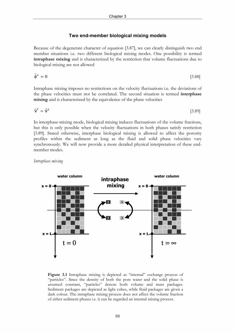
Two end-member biological mixing models Because of the degenerate character of equation [3.87], we can clearly distinguish two end member situations i.e. two different biological mixing modes. One possibility is termed intraphase mixing and is characterized by the restriction that volume fluctuations due to biological mixing are not allowed

0αφ = [3.88] Intraphase mixing imposes no restrictions on the velocity fluctuations i.e. the deviations of the phase velocities must not be correlated. The second situation is termed interphase mixing and is characterized by the equivalence of the phase velocities f sv v= [3.89]

In interphase-mixing mode, biological mixing induces fluctuations of the volume fractions, but this is only possible when the velocity fluctuations in both phases satisfy restriction [3.89]. Stated otherwise, interphase biological mixing is allowed to affect the porosity profiles within the sediment as long as the fluid and solid phase velocities vary synchronously. We will now provide a more detailed physical interpretation of these end-member modes. Intraphase mixing

Figure 3.1 Intraphase mixing is depicted as “internal” exchange process of “particles”. Since the density of both the pore water and the solid phase is assumed constant, “particles” denote both volume and mass packages. Sediment packages are depicted as light cubes, while fluid packages are given a dark colour. The intraphase mixing process does not affect the volume fraction of either sediment phases i.e. it can be regarded an internal mixing process.

intraphase mixing

x = L

x = 0

2

1

2

1

x = L

x = 0

water columnwater column

t = ∞t 0=

intraphase mixing

x = L

x = 0

2

1

2

1

x = L

x = 0

water columnwater column

t = ∞t 0=

A non-steady state model of early diagenesis

89

In intraphase-mixing mode, the activity of the benthic organisms essentially generates random fluctuations in the phase velocity, but does not induce fluctuations in the volume fractions. Translated in terms of material “particles” this implies that such particles are allowed to move, but this movement must not affect the phase distribution in the sediment. Thus by necessity, exchange processes must be “internal” to their respective phases, and consequently this particular model of biological mixing was rightfully given the label “intraphase” mixing. The mechanism of intraphase mixing is illustrated in figure [3.1]. In the intraphase-mixing mode, the organism displaces one package of fluid (or solid) and replaces it with another package of fluid (or solid) from somewhere nearby. Fluid particles can only be exchanged for fluid particles and solid particles can only be exchanged for other solid particles. Consequently, this transfer process will not affect the porosity distribution. Interphase mixing

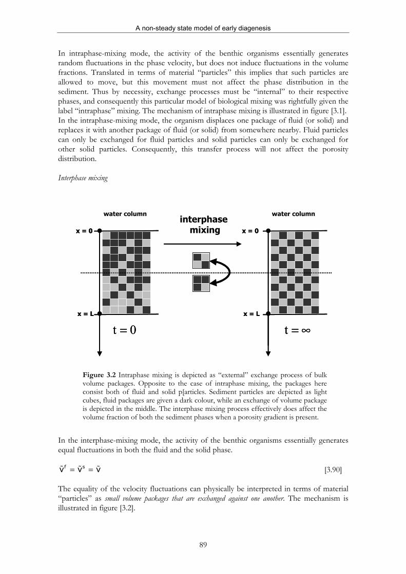
Figure 3.2 Intraphase mixing is depicted as “external” exchange process of bulk volume packages. Opposite to the case of intraphase mixing, the packages here consist both of fluid and solid p[articles. Sediment particles are depicted as light cubes, fluid packages are given a dark colour, while an exchange of volume package is depicted in the middle. The interphase mixing process effectively does affect the volume fraction of both the sediment phases when a porosity gradient is present.

In the interphase-mixing mode, the activity of the benthic organisms essentially generates equal fluctuations in both the fluid and the solid phase. f sv v v= = [3.90]

The equality of the velocity fluctuations can physically be interpreted in terms of material “particles” as small volume packages that are exchanged against one another. The mechanism is illustrated in figure [3.2].

interphase mixing

x = L

x = 0

x = L

water column

t = ∞t 0=

x = 0

water columninterphase

mixing

x = L

x = 0

x = L

water column

t = ∞t 0=

x = 0

water column

Chapter 3

90

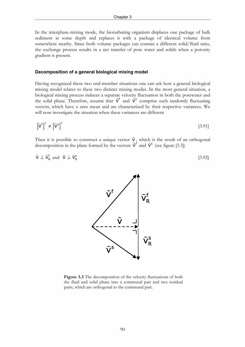
In the interphase-mixing mode, the bioturbating organism displaces one package of bulk sediment at some depth and replaces it with a package of identical volume from somewhere nearby. Since both volume packages can contain a different solid/fluid ratio, the exchange process results in a net transfer of pore water and solids when a porosity gradient is present. Decomposition of a general biological mixing model Having recognized these two end-member situations one can ask how a general biological mixing model relates to these two distinct mixing modes. In the most general situation, a biological mixing process induces a separate velocity fluctuation in both the porewater and the solid phase. Therefore, assume that fv and sv comprise such randomly fluctuating vectors, which have a zero mean and are characterized by their respective variances. We will now investigate the situation when these variances are different

2 2f sv v≠ [3.91]

Then it is possible to construct a unique vector v , which is the result of an orthogonal decomposition in the plane formed by the vectors fv and sv (see figure [3.3])

fRv v⊥ and s

Rv v⊥ [3.92]

Figure 3.3 The decomposition of the velocity fluctuations of both the fluid and solid phase into a communal part and two residual parts, which are orthogonal to the communal part.

sv

fv

v

fRv

sRv

sv

fv

v

fRv

sRv

A non-steady state model of early diagenesis

91

As a result, we can derive a unique decomposition of the phase velocity fluctuation vα in a communal part v and a residual part Rv

α

Rv v vα α= + [3.93] where the residual vectors f

Rv and sRv constitute parallel vectors. Because of the

Pythagoras‘s conjecture, the variances of these fluctuations will meet following relation

2 22Rv v vα α= + [3.94]

Combining the previous expression with [3.91] we obtain

2 2f sR Rv v≠ [3.95]

Upon substitution of the decomposition [3.93] into the earlier derived constraint [3.87], one obtains a reformulation of this constraint in terms of the residual fluctuations

( ) 0f f sR Rv vφ − = [3.96]

Given expression [3.95] and given the fact that both residual velocity fluctuations are parallel vectors, the only possibility for [3.96] to hold is when 0fφ = . Stated otherwise, the residual velocity fluctuations must not induce fluctuations in the volume fraction of the phases. Summarizing, we obtain that an arbitrary set of phase velocity fluctuations in the fluid and solid phase can be decomposed in a communal part, which is allowed to affect porosity, and a residual part, which is not allowed to affect porosity. Reverting back to the biological fluxes constituting the biological mixing model, then upon substitution of the decomposition [3.93] we obtain

( )bioR RJ v v v v vα α α α α α

φ = φ + = φ + φ = φ [3.97]

( ) ( )bio,i ii i R R i i RJ C v v C v v C v C v C v

α α α α αα α α α α α α α α= φ + + φ + = φ + φ + φ [3.98] Equation [3.98] shows that the species mass flux bio,

iJα can be decomposed into two

separate components, each corresponding to an end-member mixing mode bio, int ra, int er,i i iJ J Jα α α= + [3.99]

where the flux int raCJ due to intraphase mixing and the flux int erCJ due to interphase mixing are defined as int er bio

i iC i iJ C v C v C J C vα α α αα α α

φ= φ + φ = + φ [3.100] int raC i RJ C v

α α α= φ [3.101] In the next section we will investigate particular constitutive expressions for both the intraphase and the interphase flux in a one-dimensional setting.

Chapter 3

92

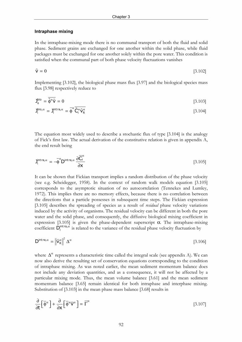
Intraphase mixing In the intraphase-mixing mode there is no communal transport of both the fluid and solid phase. Sediment grains are exchanged for one another within the solid phase, while fluid packages must be exchanged for one another solely within the pore water. This condition is satisfied when the communal part of both phase velocity fluctuations vanishes

0v = [3.102] Implementing [3.102], the biological phase mass flux [3.97] and the biological species mass flux [3.98] respectively reduce to

0bioJ vαφ = φ = [3.103] bio, int ra,i i i RJ J C v

αα α α α= = φ [3.104] The equation most widely used to describe a stochastic flux of type [3.104] is the analogy of Fick’s first law. The actual derivation of the constitutive relation is given in appendix A, the end result being

iint ra, int ra,i

CJ D

x

ααα α ∂= −φ

∂ [3.105]

It can be shown that Fickian transport implies a random distribution of the phase velocity (see e.g. Scheidegger, 1958). In the context of random walk models equation [3.105] corresponds to the asymptotic situation of no autocorrelation (Tennekes and Lumley, 1972). This implies there are no memory effects, because there is no correlation between the directions that a particle possesses in subsequent time steps. The Fickian expression [3.105] describes the spreading of species as a result of residual phase velocity variations induced by the activity of organisms. The residual velocity can be different in both the pore water and the solid phase, and consequently, the diffusive biological mixing coefficient in expression [3.105] is given the phase-dependent superscript α. The intraphase-mixing coefficient int ra,

iDα is related to the variance of the residual phase velocity fluctuation by

2int ra,

RD vα α α= ∆ [3.106] where α∆ represents a characteristic time called the integral scale (see appendix A). We can now also derive the resulting set of conservation equations corresponding to the condition of intraphase mixing. As was noted earlier, the mean sediment momentum balance does not include any deviation quantities, and as a consequence, it will not be affected by a particular mixing mode. Thus, the mean volume balance [3.61] and the mean sediment momentum balance [3.65] remain identical for both intraphase and interphase mixing. Substitution of [3.103] in the mean phase mass balance [3.68] results in

vt x

αα α α∂ ∂ φ + φ = Γ ∂ ∂ [3.107]

A non-steady state model of early diagenesis

93

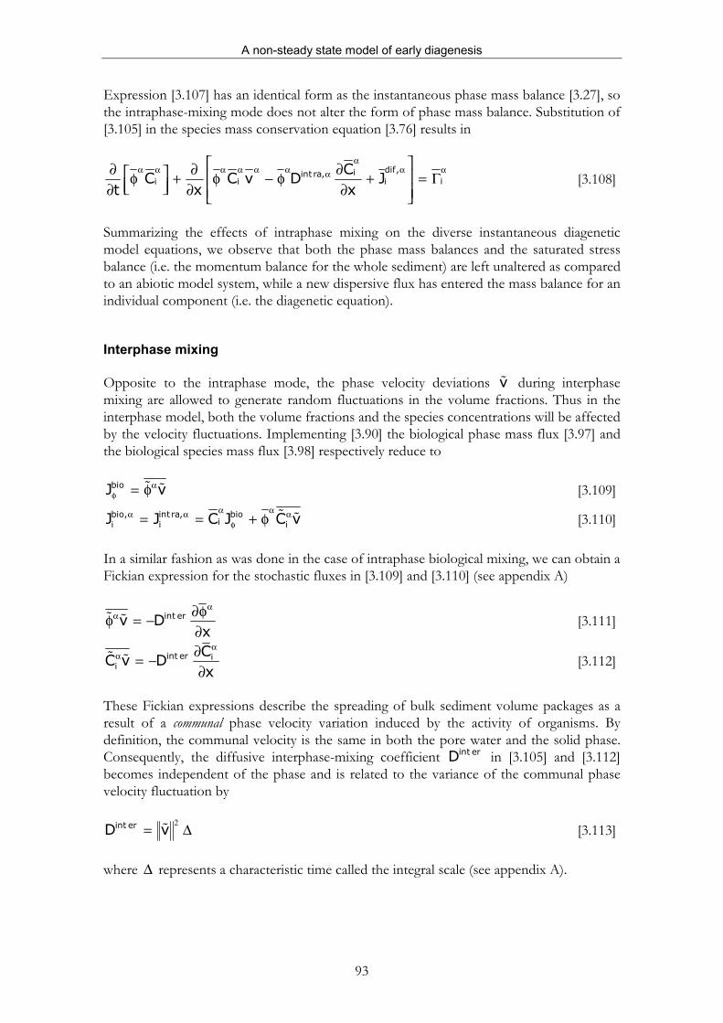
Expression [3.107] has an identical form as the instantaneous phase mass balance [3.27], so the intraphase-mixing mode does not alter the form of phase mass balance. Substitution of [3.105] in the species mass conservation equation [3.76] results in

dif,iint ra,ii i i

CC C v D J

t x x

αα α α α α α α αα

∂ ∂ ∂ φ + φ − φ + = Γ ∂ ∂ ∂ [3.108]

Summarizing the effects of intraphase mixing on the diverse instantaneous diagenetic model equations, we observe that both the phase mass balances and the saturated stress balance (i.e. the momentum balance for the whole sediment) are left unaltered as compared to an abiotic model system, while a new dispersive flux has entered the mass balance for an individual component (i.e. the diagenetic equation). Interphase mixing Opposite to the intraphase mode, the phase velocity deviations v during interphase mixing are allowed to generate random fluctuations in the volume fractions. Thus in the interphase model, both the volume fractions and the species concentrations will be affected by the velocity fluctuations. Implementing [3.90] the biological phase mass flux [3.97] and the biological species mass flux [3.98] respectively reduce to bioJ vαφ = φ [3.109] bio, int ra, bio

ii i iJ J C J C vα αα α α

φ= = + φ [3.110] In a similar fashion as was done in the case of intraphase biological mixing, we can obtain a Fickian expression for the stochastic fluxes in [3.109] and [3.110] (see appendix A)

int erv Dx

αα ∂φφ = −

∂ [3.111]

int er ii

CC v D

x

αα ∂= −

∂ [3.112]

These Fickian expressions describe the spreading of bulk sediment volume packages as a result of a communal phase velocity variation induced by the activity of organisms. By definition, the communal velocity is the same in both the pore water and the solid phase. Consequently, the diffusive interphase-mixing coefficient int erD in [3.105] and [3.112] becomes independent of the phase and is related to the variance of the communal phase velocity fluctuation by

2int erD v= ∆ [3.113] where ∆ represents a characteristic time called the integral scale (see appendix A).

Chapter 3

94

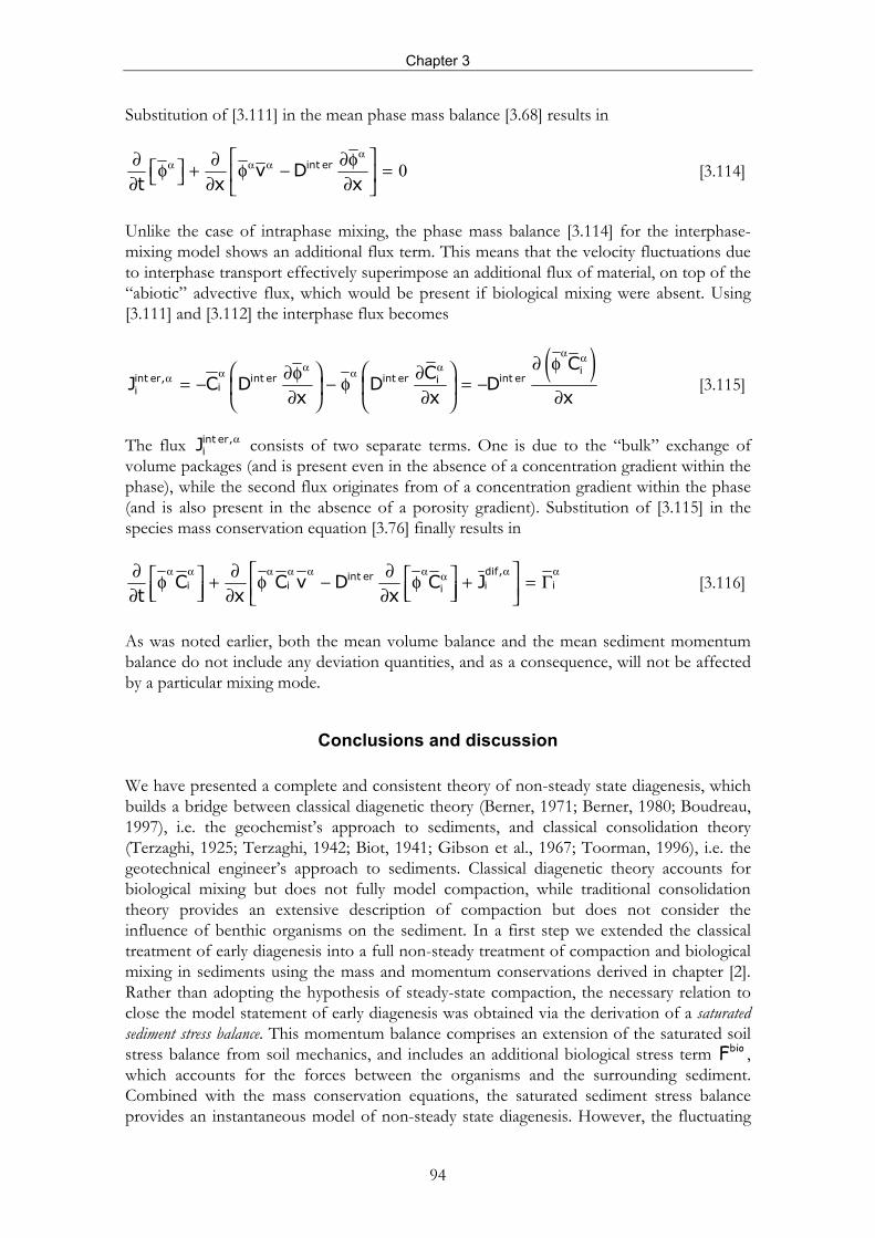
Substitution of [3.111] in the mean phase mass balance [3.68] results in

0int erv Dt x x

αα α α ∂ ∂ ∂φ φ + φ − = ∂ ∂ ∂

[3.114]

Unlike the case of intraphase mixing, the phase mass balance [3.114] for the interphase- mixing model shows an additional flux term. This means that the velocity fluctuations due to interphase transport effectively superimpose an additional flux of material, on top of the “abiotic” advective flux, which would be present if biological mixing were absent. Using [3.111] and [3.112] the interphase flux becomes

( )iint er, int er int er int eri

ii

CCJ C D D D

x x x

α αα αα αα

∂ φ ∂φ ∂= − − φ = − ∂ ∂ ∂ [3.115]

The flux int er,

iJα consists of two separate terms. One is due to the “bulk” exchange of

volume packages (and is present even in the absence of a concentration gradient within the phase), while the second flux originates from of a concentration gradient within the phase (and is also present in the absence of a porosity gradient). Substitution of [3.115] in the species mass conservation equation [3.76] finally results in

dif,int erii i iiC C v D C J

t x x

α α α α α α α αα∂ ∂ ∂ φ + φ − φ + = Γ ∂ ∂ ∂ [3.116]

As was noted earlier, both the mean volume balance and the mean sediment momentum balance do not include any deviation quantities, and as a consequence, will not be affected by a particular mixing mode.

Conclusions and discussion We have presented a complete and consistent theory of non-steady state diagenesis, which builds a bridge between classical diagenetic theory (Berner, 1971; Berner, 1980; Boudreau, 1997), i.e. the geochemist’s approach to sediments, and classical consolidation theory (Terzaghi, 1925; Terzaghi, 1942; Biot, 1941; Gibson et al., 1967; Toorman, 1996), i.e. the geotechnical engineer’s approach to sediments. Classical diagenetic theory accounts for biological mixing but does not fully model compaction, while traditional consolidation theory provides an extensive description of compaction but does not consider the influence of benthic organisms on the sediment. In a first step we extended the classical treatment of early diagenesis into a full non-steady treatment of compaction and biological mixing in sediments using the mass and momentum conservations derived in chapter [2]. Rather than adopting the hypothesis of steady-state compaction, the necessary relation to close the model statement of early diagenesis was obtained via the derivation of a saturated sediment stress balance. This momentum balance comprises an extension of the saturated soil stress balance from soil mechanics, and includes an additional biological stress term bioF , which accounts for the forces between the organisms and the surrounding sediment. Combined with the mass conservation equations, the saturated sediment stress balance provides an instantaneous model of non-steady state diagenesis. However, the fluctuating

A non-steady state model of early diagenesis

95

activity of the organisms renders the biological stress term bioF a highly variable nature and thus, the instantaneous diagenetic model only provides a mathematical snapshot of a fluctuating sediment environment. For practical purposes, it is impossible (let alone desirable) to integrate the instantaneous diagenetic model. Therefore, we developed a stochastic analysis for the instantaneous model, which closely resembles the treatment of turbulence in fluids. Rather than providing an explicit expression for bioF , the biological stress term was considered a fluctuating property, which causes random variations in the velocity of the porewater and the solid sediment. Eventually, time-averaged model equations were derived, which can be used to model early diagenesis on a time-scale of interest for practical model applications. The time-averaged mass conservation equation for both the porewater and the solid phase becomes

0biov Jt

αα αφ

∂ φ + ∇ ⋅ φ + = ∂ [3.117]

This equation includes an additional advective flux bioJφ , generated by the process of interphase mixing, which is given by bioJ vαφ = φ [3.118]

The mean diagenetic equation for a particular species becomes

md int ra, int er,ii i i i iC C v J J J

t

α α α α α αα α∂ φ + ∇ ⋅ φ + + + = Γ ∂ [3.119]

This equation includes two additional fluxes as a result of the time-averaging process, one due to intraphase mixing flux int ra,

iJα and one interphase mixing flux int er,

iJα . Both fluxes

are defined in terms of fluctuations as int er, bio

ii iJ C J C vα αα α

φ= + φ [3.120] int ra,i i RJ C v

αα α α= φ [3.121] The form of the mean volume balance and the mean sediment momentum balance does not change upon time-averaging, and as a result these balances are not influenced by a particular mixing mode.

1f sφ + φ = [3.122]

( )s s s s fs

kv U g z

′∂σ= + ∇φ + φ ρ − ρ ∇ µ ∂φ

[3.123]

An important result was that the stochastic approach eventually provided a mechanistic justification for the inclusion of the biological flux αbio,

iJ in the diagenetic equation. In the time-averaged model the biological flux αbio,

iJ appears de novo in the diagenetic equation as a correlation between velocity and concentration/porosity fluctuations, induced by biological stress term factor bioF , which is a fluctuating forcing function. Moreover, it was

Chapter 3

96

proven that this biological flux αbio,iJ could be uniquely decomposed into a part due to

intraphase mixing and a part due to interphase mixing. bio, int ra, int er,i i iJ J Jα α α= + [3.124]

This way, the stochastic analysis also provided a resolution for a long-standing problem in biological mixing theory, i.e. the inconsistency surrounding the intraphase mixing and interphase-mixing modes. Due to the uncertainty on the proper form of αbio,

iJ , there are currently two different approaches to model concentration profiles of radiotracers in surface sediments (e.g. Christensen, 1983; Officer and Lynch, 1983; Boudreau, 1986a; Fukimori et al., 1992; Mulsow et al, 1998). Applied to the same dataset, these two approaches extract deviating parameter values for accumulation and mixing processes. The expressions presented here make an end to this confusion.

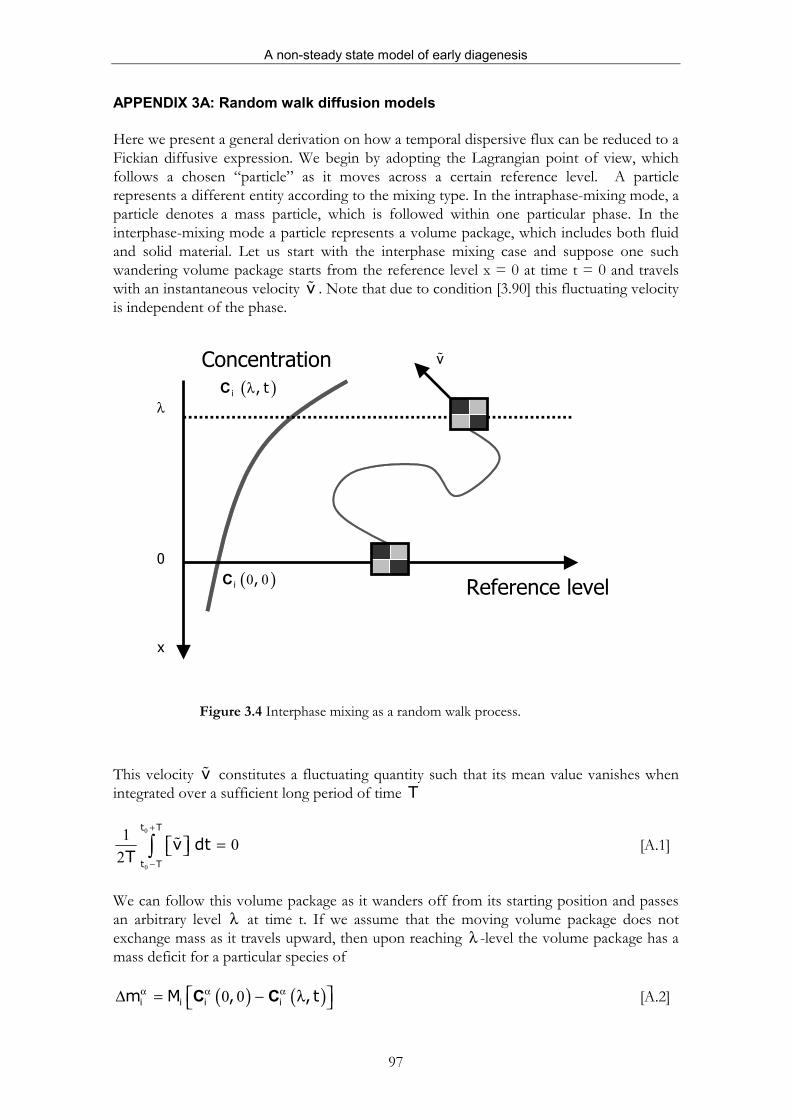
A non-steady state model of early diagenesis

97

APPENDIX 3A: Random walk diffusion models Here we present a general derivation on how a temporal dispersive flux can be reduced to a Fickian diffusive expression. We begin by adopting the Lagrangian point of view, which follows a chosen “particle” as it moves across a certain reference level. A particle represents a different entity according to the mixing type. In the intraphase-mixing mode, a particle denotes a mass particle, which is followed within one particular phase. In the interphase-mixing mode a particle represents a volume package, which includes both fluid and solid material. Let us start with the interphase mixing case and suppose one such wandering volume package starts from the reference level x = 0 at time t = 0 and travels with an instantaneous velocity v . Note that due to condition [3.90] this fluctuating velocity is independent of the phase.

Figure 3.4 Interphase mixing as a random walk process.

This velocity v constitutes a fluctuating quantity such that its mean value vanishes when integrated over a sufficient long period of time T

0

0

1 02

t T

t T

v dtT

+

−

= ∫ [A.1]

We can follow this volume package as it wanders off from its starting position and passes an arbitrary level λ at time t. If we assume that the moving volume package does not exchange mass as it travels upward, then upon reaching λ -level the volume package has a mass deficit for a particular species of

( ) ( )0 0i i i im M , , tα α α ∆ = − λ C C [A.2]

Reference level ( )0 0i ,C

x

v

λ

0

( )i , tλC

Concentration

Chapter 3

98

In expression [A.2], iM denotes the molecular mass and iαC represents the bulk

concentration. Since we are considering small but rapid fluctuations, this mass deficit per unit of volume may be approximated by the first term in a Taylor expansion

0

ii i

x

m Mx

αα

=

∂∆ = −λ∂C [A.3]

where the gradient is taken at reference level. The fluctuating movement of the volume packages induces a volume transport across the reference level. The volume transported by one moving parcel in the x-direction - per unit of area and per unit of time - is expressed by x-component the fluctuating velocity ( )v t . If we now take the average over all moving packages that start from the reference level, denoted by the brackets , we obtain the average mass flux across the reference level

( )irm, i ii iJ v v t v

x x

α αα α ∂ ∂= = − λ = − λ

∂ ∂C CC [A.4]

Examining expression [A.4], we still need to find an appropriate expression for the last term. If we consider how the value λ increases as the moving point travels away from the reference level

( )0

t

v t dt′ ′λ = ∫ [A.5]

then we can write (Taylor, 1921; Tennekes and Lumley, 1972)

( ) ( )0

t

v v t v t dt′ ′λ = ∫ [A.6]

The velocity v can be taken inside the integral because it is independent of t′ . Moreover, the averaging process can be carried out, because it is done over many moving volume packages and not over time. Since the velocity is assumed a stationary variable, the origin of the time is irrelevant, so that the correlation between ( )v t and ( )v t′ should only depend on the time difference t t′τ = − [A.7]

If we introduce the correlation coefficient

( ) ( ) ( )( ) ( )v t v t

cv t v t

′τ = [A.8]

Substituting [A.8] in [A.6], we obtain

( )2

0

t

v v c dλ = τ τ∫ [A.9]

A non-steady state model of early diagenesis

99

The correlation coefficient ( )c τ decreases as the time interval τ increases. At large values of τ the velocities ( )v t and ( )v t′ should become uncorrelated. If τ rapidly decreases and the time interval t involved in [A.9] is large enough to make the correlation coefficient zero, then it is possible to approximate the integral

( ) ( )0 0

∞

τ τ ≈ τ τ = ∆∫ ∫t

int erc d c d [A.10]

The time factor ∆int er is called the Lagrangian time-scale, because it relates to moving points (here moving volume parcels). A detailed derivation and discussion of [A.10] can be found in Tennekes and Lumley (1972). Using the Lagrangian timescale, we obtain

2v vλ = Γ [A.11] If we introduce the Root Mean Square (RMS) velocity in the x-direction

2v v= [A.12] then we can finally define a diffusion coefficient int erD as

2= ∆int er int erD v [A.13] Recall that the biological mixing coefficient does not depend on any phase-specific quantity. A second important observation is that it can vary with depth (as v can vary with depth), but at any depth the biological mixing coefficient must be the same for both the fluid and the solid phase. We can summarize the whole derivation as

( ) ( )iint er, int er int eri ii i

CJ v v t D D

x x x

α αα αα α

∂ φ∂ ∂= = − λ = − = −∂ ∂ ∂C CC [A.14]

In a similar way one can prove that

( ) int erJ v v t Dx x

α αα α αφ

∂φ ∂φ= φ = − λ = −∂ ∂

[A.15]

( )int ra, int ra,i ii i R R

C CJ C v v t D

x x

α αα α α α α α α α∂ ∂= φ = −φ λ = −φ

∂ ∂ [A.16]

then we can finally define a diffusion coefficient int ra,D α as

2α α α= ∆int ra, int ra,RD v [A.17]

Ultimately one obtains that the biological mixing coefficient for intraphase mixing becomes phase dependent, as was stressed earlier in this communication.